Figure 1. Cubic stylization deforms a given 3D shape into the style of a cube while maintaining textures and geometric features. This can be used as a non-realistic modeling tool for creating stylized 3D virtual world. We obtain 3D assets from sketchfab.com by smeerws and Jesús Orgaz licensed under CC BY 4.0.

Cubic Stylization

Abstract.

We present a 3D stylization algorithm that can turn an input shape into the style of a cube while maintaining the content of the original shape. The key insight is that cubic style sculptures can be captured by the as-rigid-as-possible energy with an ${\ell^{1}}$-regularization on rotated surface normals. Minimizing this energy naturally leads to a detail-preserving, cubic geometry. Our optimization can be solved efficiently without any mesh surgery. Our method serves as a non-realistic modeling tool where one can incorporate many artistic controls to create stylized geometries.

1. Introduction

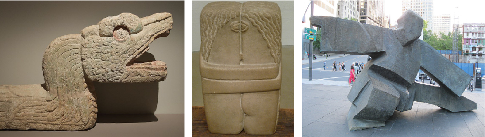
Figure 2. The cubic style have been attracting artists’ attention over centuries, such as the Serpend à’ Plumes found in Chichén Itzá (left), The Kiss by Constantin Brâncusi (middle), and the Taichi by Ju Ming (right). We obtain images from wikimedia.com photographed by Jebulon under CC0 1.0, from flickr.com by Art Poskanzer under CC BY 2.0, and from wikimedia.com by Jeangagnon under CC BY-SA 3.0.

The availability of image stylization filters and non-photorealistic rendering techniques has dramatically lowered the barrier of creating artistic imagery to the point that even a non-professional user can easily create stylized images. In stark contrast, direct stylization of 3D shapes or non-realistic modeling has received far less attention. In professional industries such as visual effects and video games, trained modelers are still required to meticulously create non-realistic geometric assets. This is because investigating geometric styles is more challenging due to arbitrary topologies, curved metrics, and non-uniform discretization. The scarcity of tools to generate artistic geometry remains a major roadblock to the development of geometric stylization.

In this paper, we focus on the specific style of cubic sculptures. The cubic style is prevalent across art history, for instance the ancient sculptures from the post-classic era (900-1250 CE), Maya sculptures, block statues in Egypt, and modern abstract sculptures such as the ones from Constantin Brâncusi and Ju Ming (Fig. 2). In addition, the cubic style is a popular digital art, such as the award-winning Anicube by Aditya Aryanto (Fig. 3).

Figure 3. A digital art – Anicube – by Aditya Aryanto produces cubic style images (right). Our method takes an input tiger (left) and outputs a “3D anicube” tiger while maintaining geometric details (middle). ©Aditya Aryanto (right). Used under permission.

Complementing their presence in art, cubic shapes also present themselves in fabrication and furniture purposes (Fig. 4).

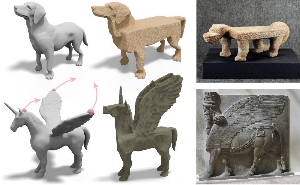
Figure 4. One can control the cubic stylization by incorporating constraints. For instance, we can fix some parts of a shape to mimic the style of a Jaguar metate from ancient Costa Rica (top) or add point constraints to mimic the Assyrian Lamassu wall sculpture (bottom). ©Antiques & Artifacts LLC (top). Used under permission.

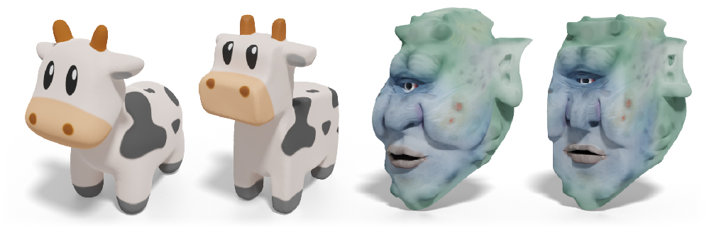
Figure 5. Our cubic stylization requires no remeshing, thus vertex attributes such as textures are preserved during the optimization. Our arap term encourges locally isometric deformations to help maintain nice textures.

We contribute to the rich history of cubic sculpting by providing a stylization tool that takes a 3D shape as input and outputs a deformed shape that has the same style as cubic sculptures.

We present cubic stylization which formulates the task as an energy optimization that naturally preserves geometric details while cubifying a shape. Our proposed energy combines an as-rigid-as-possible (arap) energy with an ${\ell^{1}}$ regularization. This energy can be minimized efficiently using the local-global approach with alternating direction method of multipliers (ADMM). This variational approach affords the flexibility of incorporating many artistic controls, such as applying constraints, non-uniform cubeness, and different global/local cube orientations (Sec. 4). Moreover, our method requires no remeshing (Fig. 5) and generalizes to polyhedral stylization (Fig. 24). Our proposed tool for non-realistic modeling goes beyond the 2D stylization and opens up the possibility of, for instance, creating non-realistic 3D worlds in virtual reality (Fig. 1).

2. Related Work

Our work shares similar motivations to a large body of work on image stylization [Kyprianidis et al., 2013], non-photorealistic rendering [Gooch and Gooch, 2001], and motion stylization [Hertzmann et al., 2009]. While their outputs are images or stylized animations, we take a 3D shape as input and output a stylized shape. Thus we focus our discussion on methods for processing geometry, including the study of geometric styles and deformation methods that share technical similarities.

Discriminative Geometric Styles

The growing interest in understanding geometric styles has been inspiring recent works on building discriminative models for style analysis. One of the main challenges is to define a similarity metric aligned with human perception. Many works propose to compare projected feature curves [Li et al., 2013; Yu et al., 2018], sub-components of a shape [Xu et al., 2010; Lun et al., 2015; Hu et al., 2017], or using learned features [Lim et al., 2016]. These models enable users to synthesize style compatible scenes [Liu et al., 2015] or transfer style components across shapes [Ma et al., 2014; Lun et al., 2016; Berkiten et al., 2017]. However, these methods are designed for discerning and transfering styles, instead of generating 3D stylized shapes directly.

Generative Geometric Styles

Direct 3D stylization has been an important topic in computer graphics. Many generative models have been proposed for producing specific styles, without relying on identifying and transferring style components from other shapes. This includes creating the collage art [Gal et al., 2007; Theobalt et al., 2007], voxel/lego art [Testuz et al., 2013; Luo et al., 2015], neuronal homunculus [Reinert et al., 2012], the manga style shapes [Shen et al., 2012], shape abstraction [Mehra et al., 2009; Kratt et al., 2014; Yumer and Kara, 2012], and bas-relief sculptures [Weyrich et al., 2007; Song et al., 2007; Kerber et al., 2009; Bian and Hu, 2011; Schüller et al., 2014]. While not pitched as stylization techniques, many geometric flows and filters can also be used for creating stylized geometry, such as creating edge-preserving smoothing geometry [Zhang et al., 2018], piece-wise planar [He and Schaefer, 2013; Stein et al., 2018b] or developable shapes [Stein et al., 2018a], and stylized shapes prescribed by image filters [Liu et al., 2018] (see Fig. 6).

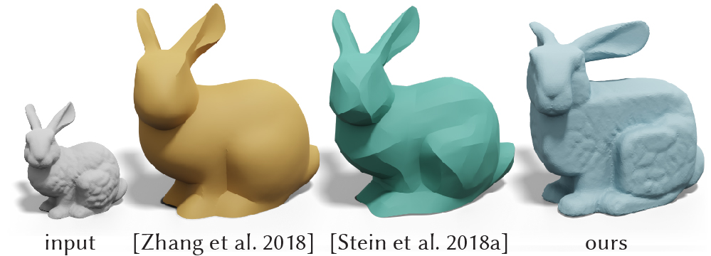
Figure 6. Our energy-based deformation shares similarities with many energy-based geometric flows and mesh filters, such as the methods of [Zhang et al., 2018] and [Stein et al., 2018a].

Our method contributes to the field of direct 3D stylization, focusing on the style of cubic sculptures (Fig. 7).

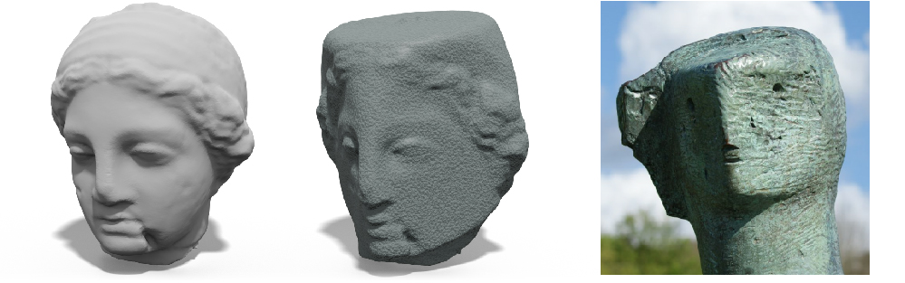
Figure 7. Cubic style sculptures are common throughout history, such as the Draped Seated Woman by Henry Moore (right). Our cubic stylization offers an instrument to create cubic geometry (middle). We obtain the the photo from flickr.com photographed by puffin11k under CC BY-SA 2.0.

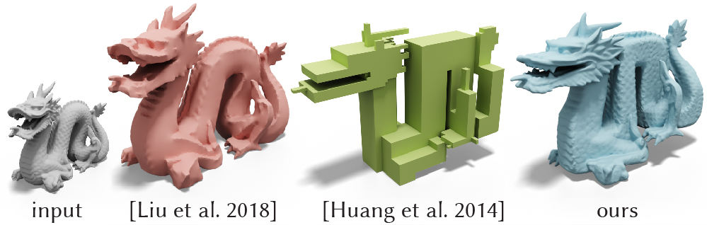
Figure 8. Paparazzi [Liu et al., 2018] with image quantization and polycube method (e.g., [Huang et al., 2014]) can create cubic style shapes (red, green), but unlike our method (blue) they do not preserve geometric details.

Shape Deformation

Many works deal with the question of how to deform shapes given modeling constraints. One of the most popular choices is the arap energy [Igarashi et al., 2005; Sorkine and Alexa, 2007; Liu et al., 2008; Chao et al., 2010], which measures local rigidity of the surface and leads to detail-preserving deformations. Not just deformations, similar formulations to arap can also be extended to other tasks such as constrained shape optimization [Bouaziz et al., 2012], parameterization [Liu et al., 2008], and simulating mass-spring systems [Liu et al., 2013]. Ever since, optimizing the arap energy has been substantially accelerated by a large amount of work, such as [Kovalsky et al., 2016; Rabinovich et al., 2017; Shtengel et al., 2017; Peng et al., 2018; Zhu et al., 2018]. However, having nearly interactive performance on highly detailed meshes still remains a major challenge. An alternative strategy to speed it up is to use the hierarchical deformation which optimizes arap on a low resolution model and then recover the original details back afterwards [Manson and Schaefer, 2011]. This class of accelerations shares similar characteristics to multiresolution modeling (see [Garland, 1999; Zorin, 2006]). We take advantage of the arap energy for detail preservation and adapt the method of Manson and Schaefer [2011] to accelerate our cubic stylization to meshes with millions of faces.

Axis-Alignment in Polycube Maps

Axis-alignment is an important property for many geometry processing tasks, such as [Muntoni et al., 2018; Stein et al., 2019]. Especially, this concept is one of the main instruments in the construction of polycube maps [Tarini et al., 2004], including defining polycube segmentations [Livesu et al., 2013; Fu et al., 2016; Zhao et al., 2018] and the cost function for polycube deformations [Gregson et al., 2011; Huang et al., 2014]. Although polycube methods can obtain cubic geometry, they fail to preserve detail (Fig. 8) because they are not desirable for intended applications such as parameterization and hexahedral meshing [Wang et al., 2007; Lin et al., 2008; Wang et al., 2008; He et al., 2009; García Fernández et al., 2013; Yu et al., 2014; Cherchi et al., 2016; Fang et al., 2016].

One tempting direction of creating cubic geometry is to use voxelization. However, voxelization fails to capture the details depicted by the artists and cannot capture the wide spectrum of cubeness across cubic sculptures. Another tempting direction is to recover geometric features from the polycube results. This would lead to a multi-step algorithm and suffer from limitations of particular detail encoding schemes (e.g., bump maps). Even if we stop the polycube

algorithm earlier such as the method of [Gregson et al., 2011] to maintain details, it does not provide a satisfactory solution (see the inset for a comparison with Fig. 5 in [Gregson et al., 2011]). More importantly, many artistic controls in Sec. 4 would be nontrivial to add on. Building stylization on top of polycube methods would also suffer from slow performance. For instance, Huang et al. [2014] propose a polycube method that minimizes the ${\ell^{1}}$-norm of the normals on the deformed tetrahedral mesh with arap for regularization. Their formulation involves minimizing a complicated non-linear function and requires minutes to hours to optimize. Thus a stylization built on top of this method would be even slower. In contrast, our formulation is a single energy optimization which can easily incorporate many artistic controls (Sec. 4). Our energy is similar to the polycube energy of [Huang et al., 2014] in that we also minimize the arap energy with a ${\ell^{1}}$ regularization, but the key difference is that we define the ${\ell^{1}}$-norm on the rotated normals of the original mesh instead. This allows us to optimize our energy much faster using the local-global approach with ADMM in only a few seconds (Table 1).

3. Method

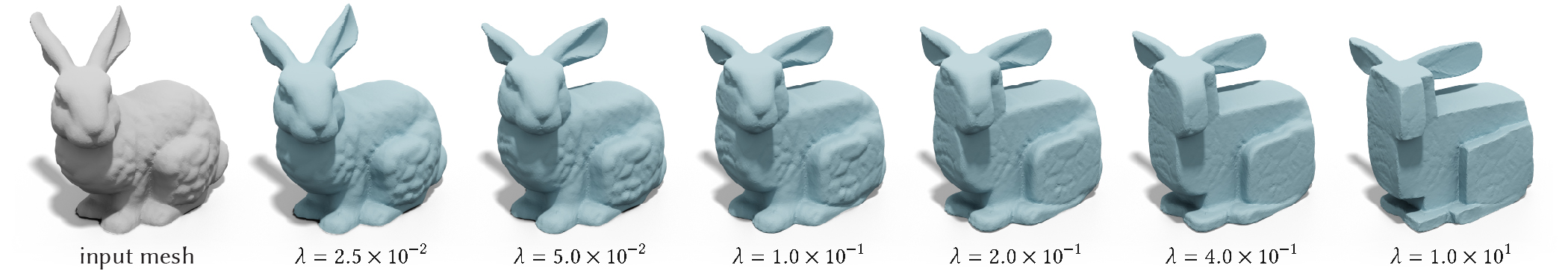
Figure 9. One can control the cubeness by changing the $λ$ parameter in Eq. 1.

The input of our method is a manifold triangle mesh with/without boundaries. Our method outputs a cubified shape where each subcomponent has the style of an axis-aligned cube. Meanwhile, our stylization will maintain the geometric details of the original mesh.

Let ${\mathsf{V}}$ be a $|{\mathsf{V}}|×3$ matrix of vertex positions at the rest state and ${\widetilde{\mathsf{V}}}$ be a $|{\mathsf{V}}|×3$ matrix containing the deformed vertex positions. We denote ${\mathsf{d}}_{ij}=[{\mathsf{v}}_{j}-{\mathsf{v}}_{i}]^{⊤}$ and ${\widetilde{\mathsf{d}}}_{ij}=[{\widetilde{\mathsf{v}}}_{j}-{\widetilde{\mathsf{v}}}_{i}]^{⊤}$ be the edge vectors between vertices $i,j$ at the rest and deformed states respectively. The energy for our cubic stylization is as follows

(1) $$\operatorname*{minimize}_{{\widetilde{\mathsf{V}}},\{{\mathsf{R}}_{i}\}}\ \sum_{i∈V}\sum_{j∈\mathcal{N}(i)}\underbrace{\frac{w_{ij}}{2}\|{\mathsf{R}}_{i}{\mathsf{d}}_{ij}-{\widetilde{\mathsf{d}}}_{ij}\|^{2}_{F}}_{{\textsc{arap}}}+\underbrace{λa_{i}\|{\mathsf{R}}_{i}\hat{\mathsf{n}}_{i}\|_{1}}_{{\textsc{cubeness}}}.$$

The first term is the arap energy [Sorkine and Alexa, 2007], where ${\mathsf{R}}_{i}$ is a $3$-by-$3$ rotation matrix, $w_{ij}$ is the cotangent weight [Pinkall and Polthier, 1993], and $\mathcal{N}(i)$ denotes the “spokes and rims” edges of the $i$th vertex [Chao et al., 2010] (see the inset). In the second term, $\hat{\mathsf{n}}_{i}$ denotes the unit area-weighted normal vector of a vertex $i$ in $\mathbb{R}^{3}$. The $a_{i}∈\mathbb{R}^{+}$ is the barycentric area of vertex $i$, which is crucial for $λ$ to exhibit the similar cubeness across different mesh resolutions.

Intuitively, minimizing the ${\ell^{1}}$-norm of the rotated normal encourages ${\mathsf{R}}_{i}\hat{\mathsf{n}}_{i}$ to align with one of coordinate axes because ${\ell^{1}}$-norm encourages sparsity. Combining the two, the optimal rotation $\{{\mathsf{R}}_{i}^{\star}\}$ would simultaneously preserve the local structure (arap) and encourage axis alignment (cubeness).

We adapt the standard local-global update strategy to optimize our energy [Sorkine and Alexa, 2007] (see Alg. 1). Our global step, updating ${\widetilde{\mathsf{V}}}$, is achieved by solving a linear system, the same as the Equation 9 in Sorkine and Alexa [2007]. Our local step, finding the optimal rotation, is however different from the previous literature due to the ${\ell^{1}}$ term.

3.1. Local-Step

Our local step for each vertex $i$ can be written as

(2) $${\mathsf{R}}^{⋆}_{i} =\operatorname*{arg\,min}_{{\mathsf{R}}_{i}∈{\text{SO}(3)}}\ \frac{1}{2}\|{\mathsf{R}}_{i}{\mathsf{D}}_{i}\ -{\widetilde{\mathsf{D}}}_{i}\|^{2}_{{\mathsf{W}}_{i}}+λa_{i}\|{\mathsf{R}}_{i}\hat{\mathsf{n}}_{i}\|_{1},$$

where ${\mathsf{W}}_{i}$ is a $|\mathcal{N}(i)|×|\mathcal{N}(i)|$ diagonal matrix of cotangent weights, ${\mathsf{D}}_{i}$ and ${\widetilde{\mathsf{D}}}_{i}$ are $3×|\mathcal{N}(i)|$ matrices of rim/spoke edge vectors at the rest and deformed states respectively. We denote $\|{\mathsf{X}}\|^{2}_{{\mathsf{Y}}}=\operatorname{Tr}({\mathsf{X}}{\mathsf{Y}}{\mathsf{X}}^{⊤})$ for notational convenience. By setting ${\mathsf{z}}={\mathsf{R}}_{i}\hat{\mathsf{n}}_{i}$, we can rewrite Eq. 2 as

(3) $$\operatorname*{minimize}_{{\mathsf{z}},{\mathsf{R}}_{i}∈{\text{SO}(3)}}\quad \frac{1}{2}\|{\mathsf{R}}_{i}{\mathsf{D}}_{i}\ -{\widetilde{\mathsf{D}}}_{i}\|^{2}_{{\mathsf{W}}_{i}}+λa_{i}\|{\mathsf{z}}\|_{1}$$

subject to $${\mathsf{z}}-{\mathsf{R}}_{i}\hat{\mathsf{n}}_{i}=0.$$

Eq. 3 is a standard ADMM formulation. We solve this local step using the scaled-form ADMM updates [Boyd et al., 2011]:

(4) $${\mathsf{R}}_{i}^{k+1} \textleftarrow\operatorname*{arg\,min}_{{\mathsf{R}}_{i}∈{\text{SO}(3)}}\frac{1}{2}\|{\mathsf{R}}_{i}{\mathsf{D}}_{i}\ -{\widetilde{\mathsf{D}}}_{i}\|^{2}_{{\mathsf{W}}_{i}}+\frac{ρ^{k}}{2}\|{\mathsf{R}}_{i}\hat{\mathsf{n}}_{i}-{\mathsf{z}}^{k}+{\mathsf{u}}^{k}\|^{2}_{2}$$

(5) $${\mathsf{z}}^{k+1} \textleftarrow\operatorname*{arg\,min}_{{\mathsf{z}}}\ λa_{i}\|{\mathsf{z}}\|_{1}+\frac{ρ^{k}}{2}\|{\mathsf{R}}_{i}^{k+1}\hat{\mathsf{n}}_{i}-{\mathsf{z}}+{\mathsf{u}}^{k}\|^{2}_{2}$$

(6) $$\tilde{{\mathsf{u}}}^{k+1} \textleftarrow{\mathsf{u}}^{k}+{\mathsf{R}}_{i}^{k+1}\hat{\mathsf{n}}_{i}-{\mathsf{z}}^{k+1}$$

(7) $$ρ^{k+1} ,{\mathsf{u}}^{k+1}\textleftarrow\textit{update\,($ρ^{k}$)}$$

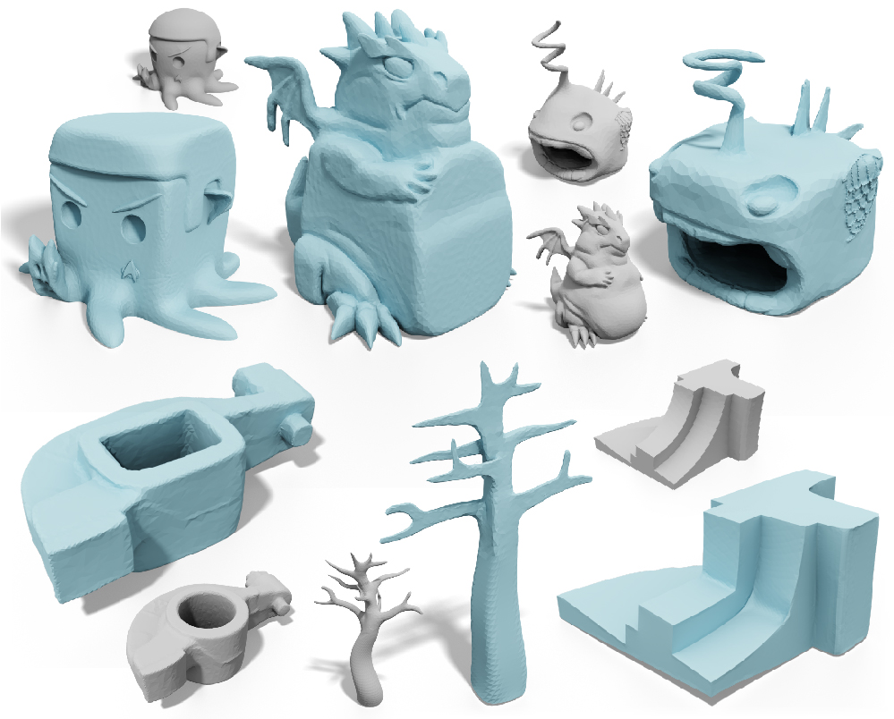
Figure 10. We turn 3D shapes into the cubic style (blue) with Alg. 1. ©Angelo Tartanian (top left), Splotchy Ink (top), Dan Slack (top right) under CC BY.

Figure 11. We can also turn meshes with boundaries (red) into the cubic style. ©Takeshi Murata (left) under CC BY.

where $ρ∈\mathbb{R}_{+}$ is the penalty and ${\mathsf{u}}$ is the scaled dual variable.

Eq. 4 is an instance of the orthogonal Procrustes [Gower et al., 2004]

$${\mathsf{R}}_{i}^{k+1}\textleftarrow\operatorname*{arg\,max}_{{\mathsf{R}}_{i}∈{\text{SO}(3)}}\ \operatorname{Tr}({\mathsf{R}}_{i}{\mathsf{M}}_{i})$$

$${\mathsf{M}}_{i}=\begin{bmatrix}{\mathsf{D}}_{i}\quad\hat{\mathsf{n}}_{i}\end{bmatrix}\begin{bmatrix}{\mathsf{W}}_{i}&\\ &ρ^{k}\end{bmatrix}\begin{bmatrix}{\widetilde{\mathsf{D}}}_{i}^{⊤}\\ ({\mathsf{z}}^{k}-{\mathsf{u}}^{k})^{⊤}\end{bmatrix}.$$

One can derive the optimal ${\mathsf{R}}_{i}$ from the singular value decomposition of ${\mathsf{M}}_{i}=\mathcal{U}_{i}Σ_{i}\mathcal{V}_{i}^{⊤}$:

(8) $${\mathsf{R}}_{i}^{k+1}\textleftarrow\mathcal{V}_{i}\mathcal{U}_{i}^{⊤},$$

up to changing the sign of the column of $\mathcal{U}_{i}$ so that $\det({\mathsf{R}}_{i})>0$.

Eq. 5 is an instance of the lasso problem [Tibshirani, 1996; Boyd et al., 2011], which can be solved with a shrinkage step:

(9) $${\mathsf{z}}^{k+1}\textleftarrow\mathcal{S}_{\nicefrac{{λa_{i}}}{{ρ^{k}}}}({\mathsf{R}}_{i}^{k+1}\hat{\mathsf{n}}_{i}+{\mathsf{u}}^{k})$$

$$\mathcal{S}_{κ}({\mathsf{x}})_{j}=(1−\nicefrac{{κ}}{{|x_{j}|}})_{+}\ x_{j}$$

We update the penalty $ρ$ (Eq. 7) according to Sec. 3.4.1 in [Boyd et al., 2011] where ${\mathsf{u}}$ needs to be rescaled accordingly after updating $ρ$.

In short, local fitting is performed by running Eq. 8, 9, 6, and 7 iteratively until the norm of primal/dual residuals are small. Warm starting the local-step parameters from the previous iteration can significantly speed up the optimization. Specifically, we initialize ${\mathsf{z}},{\mathsf{u}}$ with zeros, and set the initial $ρ=10^{-4}$, $ϵ^{\text{abs}}=10^{-5}$, $ϵ^{\text{rel}}=10^{-3}$, $μ=10$, and $τ^{\text{incr}}=τ^{\text{decr}}=2$ (the same notation as used in Sec. 3 of [Boyd et al., 2011]). Then ${\mathsf{z}},{\mathsf{u}},ρ$ are reused in consecutive iterations. Note that for extremely large $λ$ one may need to increase

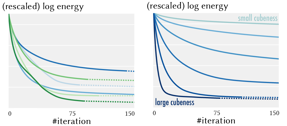
Figure 12. We show the convergence behavior of different meshes in Fig. 10 (left, blue), Fig. 16 (left, green), and different cubenesses in Fig. 9 (right). Note that the dotted line imply the optimization has stopped.

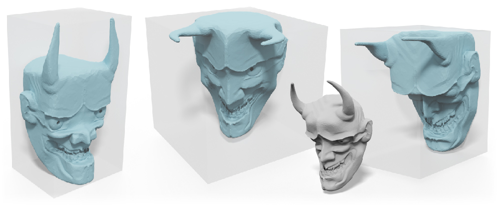
Figure 13. The global orientation of the shape influences the ${\ell^{1}}$ term in Eq. 1. Applying different rotations to the mesh lead to different results. ©My Dog Justice under CC BY.

the initial value of $ϵ^{\text{abs}}$ accordingly in order to avoid bad local minima. We stop the

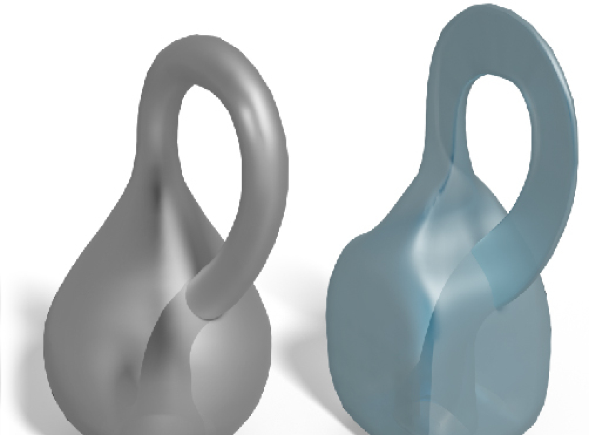
Figure 14. Our method can cubify non-orientable surfaces such as the Klein bottle.

optimization when the relative displacement, the infinity norm of relative per vertex displacements, is lower than $3×10^{-3}$ (see Fig. 12 for the convergence plots). More elaborate stopping criteria, such as the method of [Zhu et al., 2018], could also be used.

At this point we have completed the cubic stylization algorithm summarized in Alg. 1, enabling us to efficiently create cubified shapes (see Fig. 10). In Fig. 11 and 14 we show that this formulation is applicable to meshes with boundaries and non-orientable surface respectively. As the cubeness is dependent to the orientation of the mesh, one can apply different rotations to control how the stylization runs (Fig. 13). We expose the weighting $λ$ to be a design parameter controlling the cubeness of a shape (Fig. 9).

However, the “vanilla” cube stylization shares the same caveat as other distortion minimization algorithms: having slow runtime on high resolution meshes.

Input :  A triangle mesh ${\mathsf{V}},{\mathsf{F}}$

Output :  Deformed vertex positions ${\widetilde{\mathsf{V}}}$

1 ${\widetilde{\mathsf{V}}}\textleftarrow{\mathsf{V}}$

2 while not converge do

3       ${\mathsf{R}}\textleftarrow local\text{-}step\,({\mathsf{V}},{\widetilde{\mathsf{V}}},λ)$

4       ${\widetilde{\mathsf{V}}}\textleftarrow global\text{-}step\,({\mathsf{R}})$

5      

Algorithm 1 $Cube\ Stylization\,(λ)$

1

Input :  A triangle mesh ${\mathsf{V}},{\mathsf{F}}$

Output :  Deformed vertex positions ${\widetilde{\mathsf{V}}}$

// pre-processing

2 $m\textleftarrow\text{target number of faces}$

3 ${\mathsf{V}}_{c},{\mathsf{F}}_{c}\textleftarrow\textit{edge collapses}\,({\mathsf{V}},{\mathsf{F}},m)$

// cubic stylization

4 ${\widetilde{\mathsf{V}}}_{c}\textleftarrow{\mathsf{V}}_{c}$

5 while not converge do

6       ${\mathsf{R}}\ \ \textleftarrow local\text{-}step\,({\mathsf{V}}_{c},{\widetilde{\mathsf{V}}}_{c},λ)$

7       ${\widetilde{\mathsf{V}}}_{c}\textleftarrow global\text{-}step\,({\mathsf{R}})$

8      

${\widetilde{\mathsf{V}}},{\mathsf{F}}\textleftarrow\textit{affine vertex splits}\,({\widetilde{\mathsf{V}}}_{c},{\mathsf{F}}_{c})$

Algorithm 2 $Fast\ Cube\ Stylization\,(λ,m)$

3.2. Affine Progressive Meshes

Manson and Schaefer [2011] propose a hierarchical approach to accelerate arap deformations. The main idea is to deform a low-resolution model and recover the details back after convergence.

Specifically, Manson and Schaefer [2011] propose a progressive mesh [Hoppe, 1996] representation which first simplifies a given mesh via a sequence of edge collapses, and then represents the mesh as its coarsest form together with a sequence of vertex splits. After

applying some deformations to the coarsest mesh, each “deformed” vertex split is computed by fitting the best local rigid transformation. This approach is suitable for deformations that are locally rigid (e.g., arap), but our cubic stylization is less rigid for larger $λ$.

So we fit the best affine transformation in each vertex split, rather than rigid transformations. Specifically, in each edge collapse we store the displacement vectors from the newly inserted vertex ${\mathsf{p}}_{i}$ to the endpoints ${\mathsf{p}}_{j},{\mathsf{p}}_{k}$ (see the inset) together with a matrix ${\mathsf{A}}$:

$${\mathsf{A}}=({\mathsf{Q}}_{i}{\mathsf{Q}}_{i}^{⊤})^{-1}{\mathsf{Q}}_{i}.$$

${\mathsf{Q}}_{i}$ is a $3×|\mathcal{N}(i)|$ matrix where each column is the vector from ${\mathsf{p}}_{i}$ to one of its one-rings neighbors $\mathcal{N}(i)$. If $({\mathsf{Q}}_{i}{\mathsf{Q}}_{i}^{⊤})$ is singular (e.g., in planar regions), we remedy the issue with the Tikhonov regularization [Tikhonov et al., 2013]. Then ${\mathsf{A}}$ is used to computed the deformed displacements for each vertex split as

$${\widetilde{\mathsf{p}}}_{j}-{\widetilde{\mathsf{p}}}_{i}={\widetilde{\mathsf{Q}}}_{i}{\mathsf{A}}^{⊤}({\mathsf{p}}_{j}-{\mathsf{p}}_{i}),$$

where ${\widetilde{\mathsf{p}}}_{i}$ denotes the position of vertex $i$ in the cubified coarsened shape, and ${\widetilde{\mathsf{Q}}}_{i}$ is a $3×|\mathcal{N}(i)|$ matrix containing vectors from ${\widetilde{\mathsf{p}}}_{i}$ to its one-rings neighbors.

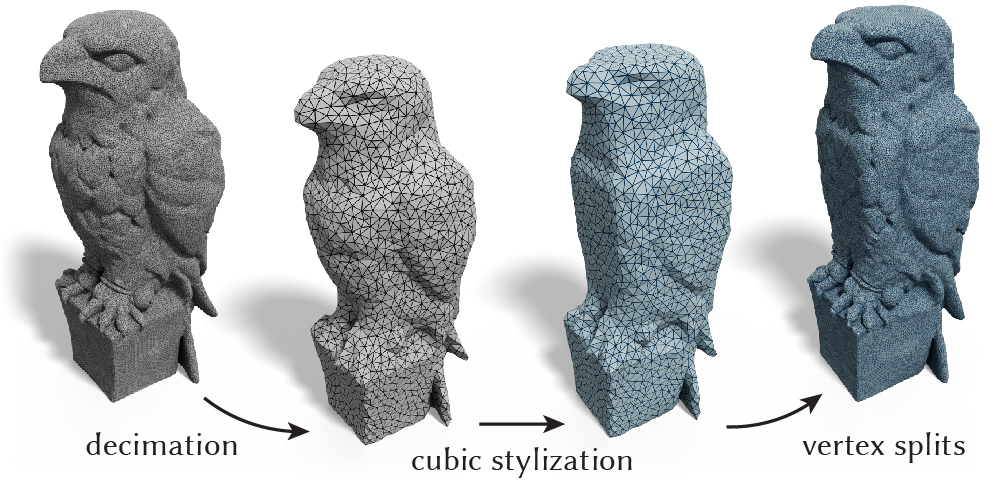
Figure 15. Affine progressive meshes allow us run cubic stylization on a low-resolution model and then recover original details when converged. ©Colin Freeman under CC BY.

Affine progressive meshes allows us to losslessly recover the original meshes undergoing affine transformations. For smooth non-affine transformations such as our cube stylization, it could still be approximately recovered (see Fig. 15). We summarize our cubic stylization with the affine progressive mesh in Alg. 2. Note that the edge collapses is just a pre-processing step. In the online stage, one only needs to run cubic stylization on the coarsest mesh and then apply a sequence of vertex splits to visualize the result on the original resolution. This offers a huge speed-up when interacting the parameter $λ$ on highly detailed models (see Fig. 16).

An interesting observation is that the number of faces $m$ in the coarsest mesh not only controls the runtime, but implicitly controls the frequency level of geometric details that gets preserved.

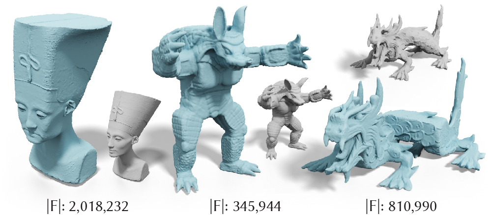
Figure 16. With the affine progressive meshes, we can scale the cubic stylization to meshes with millions of faces. The Nefertiti mesh (left) was scanned by Nora Al-Badri and Jan Nikolai Nelles from the Nefertiti bust.

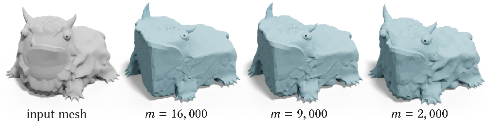
Figure 17. The number of faces $m$ used in the decimated mesh not only controls the runtime but also the frequency level of details that get preserved. ©Joseph Larson under CC BY.

In Fig. 17 we show that, under the same $λ$, a smaller $m$ keeps details across a wider frequency range; in contrast, a larger $m$ only keeps details at higher frequencies. Therefore one can manipulate the level of preserved features by playing with $m$.

3.3. Implementation

We implement the cubic stylization in C++ using libigl [Jacobson et al., 2018] and evaluate our runtime on a MacBook Pro with an Intel i5 2.3GHz processor. Table 1 lists the parameters and the runtime of our stylization in Fig. 10 (top) and Fig. 16. We test our methods on meshes in the Thingi10K [Zhou and Jacobson, 2016] and show that we can obtain stylized geometry within a few seconds. This is important for users to receive quick feedback on their parameter choices and iterate on their designs, such as the cubeness $λ$ in Fig. 9 and the the level of details $m$ in Fig. 17.

User study

We prototype a user interface (see the inset) to conduct an informal user study with six participants (4 male, 2 female) between the ages of 24 and 29. Participant 3D modeling experience ranged from none (complete novice) to three years of hobbyist use. Each participant was instructed for three minutes on how to use our software to load a mesh and control the cubeness parameter $λ$. Then we asked them to cubify a shape of their choosing from a collection of ten shapes. The results of their work is show in Fig. 18. All users reported that they were satisfied with the cubeness of their resulting shape. One user said that controlling the cubeness of their resulting shape is very easy because it only requires tuning a single parameter.

Table 1. For each example in Fig. 10 and Fig. 16, we report the number of faces in the original model ($|F|$), $l1$ weight ($λ$), number of faces of the coarsest mesh ($m$), number of iterations (Iters.), pre-processing time (Pre.), and runtime at the online stage (Runtime).

Model	$|F|$	$λ$	$m$	Iters.	Pre.	Runtime
Fig. 10, left	39K	0.20	n/a	106	n/a	$\mathbf{5.08s}$
Fig. 10, mid.	41K	0.20	n/a	93	n/a	$\mathbf{4.50s}$
Fig. 10, right	21K	0.4	n/a	86	n/a	$\mathbf{2.26s}$
Fig. 16, left	2018K	0.20	20K	83	64.19$s$	$\mathbf{3.93s}$
Fig. 16, mid.	346K	0.40	20K	222	10.69$s$	$\mathbf{4.59s}$
Fig. 16, right	811K	0.30	40K	173	30.44$s$	$\mathbf{8.38s}$

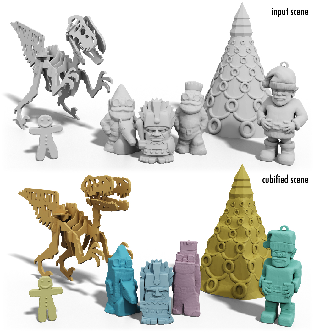
Figure 18. Even non-professional users can effortlessly turn an input scene (top) into a cubified scene (bottom). Different colors are results created by different users. From left to right, ©Peter Leppik, Cleven, TerenceKing, MakerBot, TerenceKing, PerryEngel, and Christina Chun under CC BY.

4. Artistic Controls

In addition to the two parameters $λ,m$, we expose many variants of our stylization to incorporate artistic controls. As a non-realistic modeling tool, this is important for users to realize their creativity.

We first focus our discussion on a variety of artistic controls that are related to the cubeness parameter $λ$. Although Eq. 1 only has a single $λ$ for an entire shape, we can actually specify different $λ_{i}$ for each vertex independently to have non-uniform cubeness, which leads to the expression $λ_{i}a_{i}\|{\mathsf{R}}_{i}\hat{\mathsf{n}}_{i}\|_{1}$. In Fig. 19, we use this approach to make the back of the sheep much more cubic than the rest of the shape to create an ottoman-like geometry.

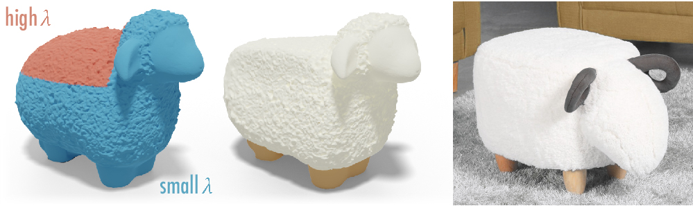
Figure 19. We vary $λ$ across the surface to have different cubeness for different parts. We apply higher $λ$ on the red region and smaller $λ$ for the blue region to create an ottoman-like shape (middle). ©pmoews under CC BY.

We can also specify the non-uniform cubeness $λ_{i}$ in a different way, instead of painting on the surface directly. In Fig. 20 we paint a function on the Gauss map in which the surface normal pointing towards left has higher cubeness. When we map this function back to the surface, we can have a cubified owl that is more cubic when initial normals pointing towards the left and less cubic when pointing towards the right.

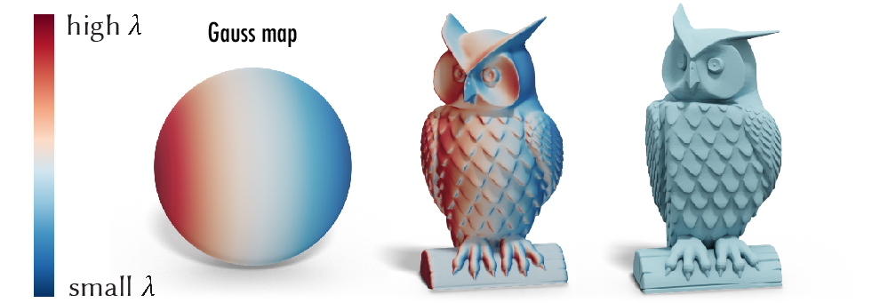
Figure 20. We can paint the $λ$ function on the Gauss map to have non-uniform $λ$ over the surface. In the figure, we have higher $λ$ for the original normals pointing towards left, and vice versa. ©Tom Cushwa under CC BY.

Similarly, we can have different $λ_{x},λ_{y},λ_{z}$ for different axes. In Fig. 21, we replace the cubeness in Eq. 1 with $a_{i}(λ_{x}|({\mathsf{R}}_{i}\hat{\mathsf{n}}_{i})_{x}|+λ_{y}|({\mathsf{R}}_{i}\hat{\mathsf{n}}_{i})_{y}|+λ_{z}|({\mathsf{R}}_{i}\hat{\mathsf{n}}_{i})_{z}|)$ and specify different values for each $λ_{x},λ_{y},λ_{z}$ to have the style of a rectangular prism.

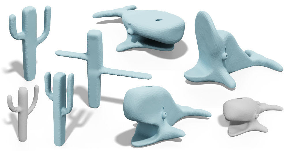
Figure 21. We can vary $λ$ for different axes to turn inputs into the biased cubic style (blue) towards x,y,z axes respectively. ©MakerBot (right) under CC BY.

If one wants to fix certain parts of the shape, we can easily add constraints in the global step, the same way as the method of Sorkine and Alexa [2007]. In Fig. 4 we add the parts constraint by fixing the position of some vertices when solving the linear system; we add the points constraint by specifying some deformed vertices ${\widetilde{\mathsf{V}}}_{i}$ at user-desired positions. We can also use the same methodology to constrain some parts of the geometry lying on certain planes. For instance, setting $({\widetilde{\mathsf{V}}}_{i})_{x}=0$ can force vertex $i$ lying on the yz-plane. In Fig. 22 we use this plane constraint to create a table clinger.

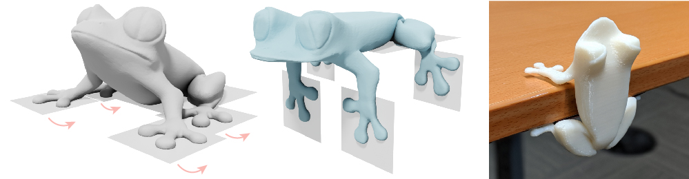
Figure 22. We constrain certain parts of the geometry lying on certain planes to create a 3D printed table clinger (right). ©Morena Protti under CC BY.

In addition, one can utilize the property of the ${\ell^{1}}$-norm to have different artistic effects. Because the cubeness term is orientation dependent, in Fig. 13 we can apply different rotations to the mesh before the stylization to control the results. Rather than rotating the mesh, another way is to encode the normal vector in a different coordinate system $λa_{i}\|{\mathsf{R}}_{i}\hat{\mathsf{n}}_{i}^{\text{local}}\|_{1}$, where we use $\hat{\mathsf{n}}_{i}^{\text{local}}$ to denote the user-desired coordinate system for vertex $i$. This perspective allows us to define the ${\ell^{1}}$-norm on different coordinate systems for different parts of the shape to obtain different cube orientations (Fig. 23).

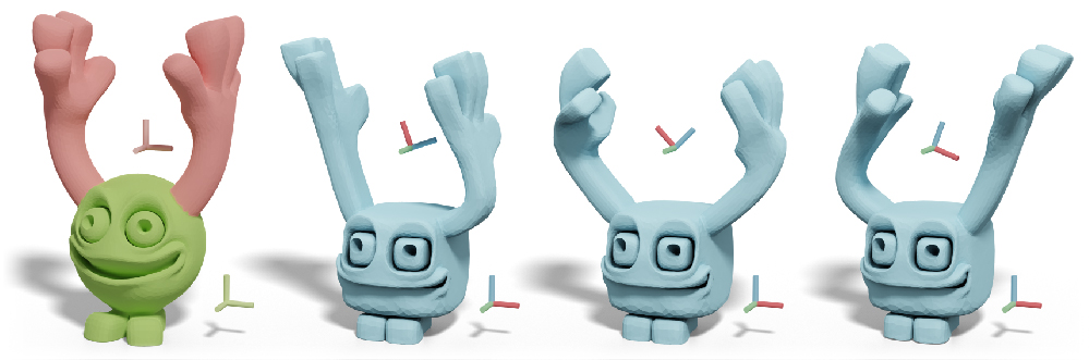
Figure 23. We can define the ${\ell^{1}}$-norm on different coordinate systems for different parts of the shape, instead of using the world coordinates. In the figure the hands and the body use different coordinate systems (left). By changing them, we can vary the cube orientations for different parts. ©David Hagemann under CC BY.

Beyond the cubic stylization, in Fig. 24, 25 we apply a coordinate transformation ${\mathsf{B}}$ inside the ${\ell^{1}}$-norm $λa_{i}\|{\mathsf{B}}{\mathsf{R}}_{i}\hat{\mathsf{n}}_{i}\|_{1}$ to achieve polyhedral stylization, for which we provide the details in App. A.

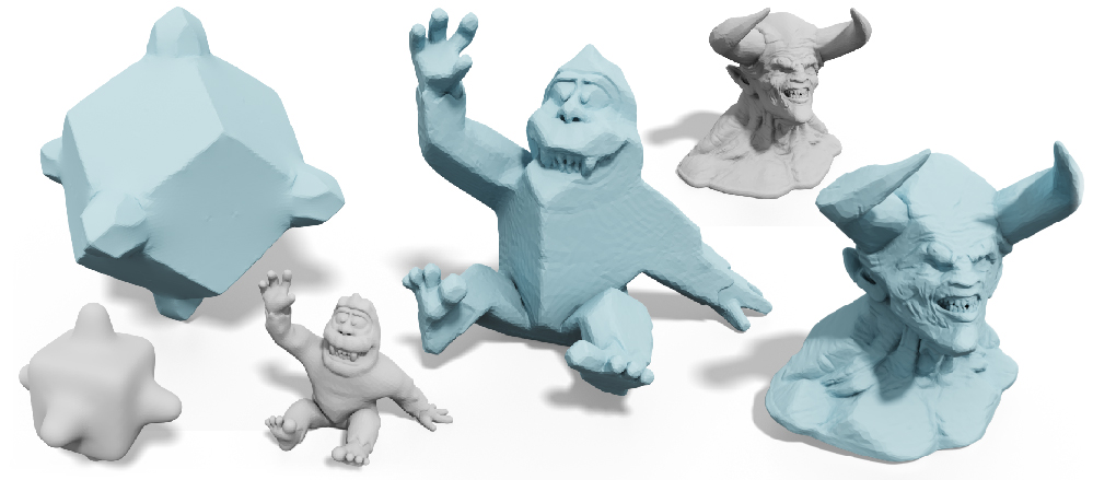
Figure 24. We apply a coordinate transformation inside the ${\ell^{1}}$-norm to generalize cubic stylization to polyhedrons. ©Proto Paradigm (middle), Ola Sundberg (right) under CC BY.

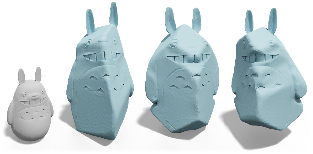
Figure 25. We apply non-symmetric coordinate transformations inside the ${\ell^{1}}$-norm to create irregular polyhedral stylization. ©Johannes under CC BY.

Once we obtain the stylized shapes, they are ready to be used by standard deformation techniques in animations (Fig. 26).

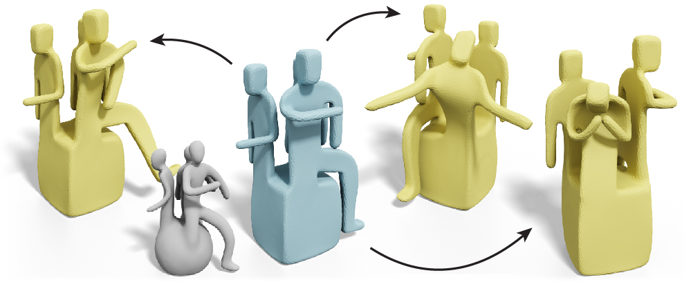
Figure 26. Once we have the cubic geometry (blue), standard deformation techniques (e.g., [Sorkine and Alexa, 2007]) can be used to manipulate the cubified shape (yellow).

5. Limitations & Future Work

Accelerating the stylization to real-time would enable faster iterations between designs. Developing a more robust stylization to for bad quality triangles, non-manifold meshes, or even point cloud could be useful for stylizing real-world geometric data. Guaranteeing results to be self-intersection free would be desirable for downstream tasks. Extending our energy to be invariant to discretizations could achieve more consistent results across different resolutions (see Fig. 27).

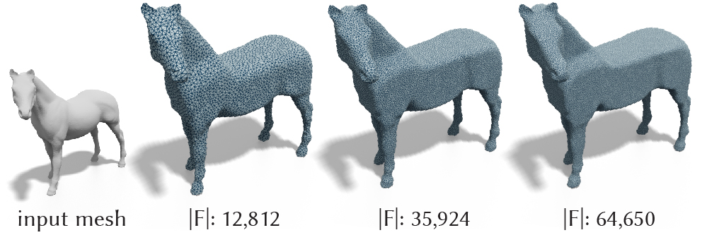
Figure 27. Although exhibiting similar cubenesses, our stylization is still not invariant to different resolutions.

Extending to quadrilateral meshes and NURBS surfaces could benefit existing modeling or engineering design softwares. Generalizing to volumetric meshes could have a better volume preservation. Exploring different deformation energies and $\ell^{p}$-norm could lead to novel stylization tools for non-realistic modeling. Beyond generating stylized shapes, the mathematical expression of the cubic geometry could offer insights toward understanding more intricate styles. For instance, Cubism has been considered as a revolutionized artistic style for paintings and sculptures. Cubism has appeared since the early 20th century. Since then, several attempts have tried to describe [Henderson, 1983] and generate Cubist art [Wang et al., 2011; Corker-Marin et al., 2018], but more efforts still required to offer scientific explanations to a wide variety of Cubist art. Our cubic stylization only focuses on a specific style. We hope this could inspire future attempts to capture different sculpting styles such as those presented in African art, or even a generic approach to create different styles in an unified framework.

Appendix A Polyhedral Generalization

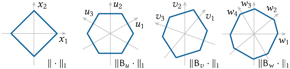
Figure 28. By specifying different coordinate transformations ${\mathsf{B}}$ inside the ${\ell^{1}}$-norm, we can encourage polyhedral style.

Simply applying a coordinate transformation $B:\mathbb{R}^{n}\textrightarrow\mathbb{R}^{m}$ inside the ${\ell^{1}}$-norm can encourage polyhedral results, instead of cubic results (see Fig. 28). The ${\ell^{1}}$-norm of a vector is defined as the summation of its magnitudes along each basis vector. Thus applying a coordinate transformation inside the ${\ell^{1}}$-norm changes its bahavior because the basis vectors are different. Following the notation in Eq. 1, polyhedron energy can be written as

$$\operatorname*{minimize}_{{\widetilde{\mathsf{V}}},\{{\mathsf{R}}_{i}\}}\ \sum_{i∈V}\sum_{j∈\mathcal{N}(i)}\frac{w_{ij}}{2}\|{\mathsf{R}}_{i}{\mathsf{D}}_{ij}-{\widetilde{\mathsf{D}}}_{ij}\|^{2}_{F}+λa_{i}\|{\mathsf{B}}{\mathsf{R}}_{i}\hat{\mathsf{n}}_{i}\|_{1}.$$

In our case, ${\mathsf{B}}$ is a $m$-by-$3$ coordinate transformation matrix for shapes embedded in $\mathbb{R}^{3}$. Again by setting ${\mathsf{z}}={\mathsf{R}}_{i}\hat{\mathsf{n}}_{i}$ we can reach almost the same optimization procedures, except the Eq. 5 now becomes (we ignore the iteration superscript for clarity)

(10) $${\mathsf{z}}^{k+1}\textleftarrow\operatorname*{arg\,min}_{{\mathsf{z}}}\ λa_{i}\|{\mathsf{B}}{\mathsf{z}}\|_{1}+\frac{ρ}{2}\|{\mathsf{R}}_{i}\hat{\mathsf{n}}_{i}-{\mathsf{z}}+{\mathsf{u}}\|^{2}_{2}.$$

Similar to common techniques for solving the Basis Pursuit problem, we introduce a variable ${\mathsf{t}}\succeq\|{\mathsf{B}}{\mathsf{z}}\|_{1}$ to transform Eq. 10 into a small quadratic program subject to equality constraints

$$\operatorname*{minimize}_{{\mathsf{z}},{\mathsf{t}}}\ \begin{bmatrix}{\mathsf{z}}^{⊤}\ {\mathsf{t}}^{⊤}\end{bmatrix}\begin{bmatrix}\nicefrac{{ρ}}{{2}}\cdot\mathsf{I}_{3}&\mathsf{0}\\ \mathsf{0}&\mathsf{0}\end{bmatrix}\begin{bmatrix}{\mathsf{z}}\\ {\mathsf{t}}\end{bmatrix}$$

$$\qquad+\begin{bmatrix}-ρ({\mathsf{R}}_{i}\hat{\mathsf{n}}_{i}+{\mathsf{u}})^{⊤}\ λa_{i}\mathsf{1}_{m}^{⊤}\end{bmatrix}\begin{bmatrix}{\mathsf{z}}\\ {\mathsf{t}}\end{bmatrix}$$

subject to $$\begin{bmatrix}{\mathsf{B}}&-\mathsf{I}_{m}\\ -{\mathsf{B}}&-\mathsf{I}_{m}\end{bmatrix}\begin{bmatrix}{\mathsf{z}}\\ {\mathsf{t}}\end{bmatrix}\preceq\mathsf{0},$$

where $\mathsf{I}_{x}$ and $\mathsf{1}_{x}$ denote the identity matrix with size $x$ and a column vector of $1$ with size $x$ respectively. We then solve this efficiently using cvxgen [Mattingley and Boyd, 2012]. Note that the results in Fig. 24 and Fig. 25 use $m=4$.