Edge theories of 2D fermionic symmetry protected topological phases protected by unitary Abelian symmetries

Abstract

Abelian Chern-Simons theory, characterized by the so-called $K$ matrix, has been quite successful in characterizing and classifying Abelian fractional quantum hall effect (FQHE) as well as symmetry protected topological (SPT) phases, especially for bosonic SPT phases. However, there are still some puzzles in dealing with fermionic SPT(fSPT) phases. In this paper, we utilize the Abelian Chern-Simons theory to study the fSPT phases protected by arbitrary Abelian total symmetry $G_{f}$. Comparing to the bosonic SPT phases, fSPT phases with Abelian total symmetry $G_{f}$ has three new features: (1) it may support gapless majorana fermion edge modes, (2) some nontrivial bosonic SPT phases may be trivialized if $G_{f}$ is a nontrivial extention of bosonic symmetry $G_{b}$ over $\mathbb{Z}_{2}^{f}$, (3) certain intrinsic fSPT phases can only be realized in interacting fermionic system. We obtain edge theories for various fSPT phases, which can also be regarded as conformal field theories (CFT) with proper symmetry anomaly. In particular, we discover the construction of Luttinger liquid edge theories with central charge $n-1$ for Type-III bosonic SPT phases protected by $(\mathbb{Z}_{n})^{3}$ symmetry and the Luttinger liquid edge theories for intrinsically interacting fSPT protected by unitary Abelian symmetry. The ideas and methods used in these examples could be generalized to derive the edge theories of fSPT phases with arbitrary unitary Abelian total symmetry $G_{f}$.

I Introduction

Recently, tremendous progress has been made towards understanding gapped phases of quantum matter. It has been pointed out that the entanglement pattern is a unique feature to characterize gapped quantum phases. A state only has “short-range entanglement” if and only if it can be connected to an un-entangled state (i.e., a direct product state or an atomic insulator state) via a local unitary transformation; otherwise, it has ”long-range entanglement”. In the presence of global symmetry, even the ”short-range entangled” phases can have many different classes. Among them one class is the conventional symmetry breaking phase described by the Landau theory. However, to our surprise, there exists a new class of topological phases - the symmetry protected topological (SPT) phases[1, 2, 3] associated with any global symmetry in any dimension. So far, the SPT phases have been quite well-understood in many aspects for both interacting bosonic and fermionic systems, including the classification[2, 3, 4, 5, 6, 7, 8, 9, 10, 6, 11, 12, 13, 14, 15, 16], characterization[17, 18, 19, 20, 21, 22, 23, 24, 25, 26, 27, 16, 28], boundary-bulk correspondence[29, 30, 31, 32, 33, 34, 35, 36, 37, 38, 39, 40], construction of exactly solvable models[41, 42, 2, 3, 17, 4, 43, 44, 45], field theories[7, 46, 12, 47, 15, 48, 49], model realization[50, 51, 52, 53, 54, 55] and experimental discovery[56] as well. One of the most striking phenomena of SPT phase is that even though the bulk is short-range entangled without any fractionalized excitation, its boundary can not be short-range entangled symmetric gapped state. It must be gapless, breaking symmetry(spontaneously or explicitly) or topological ordered state(for the boundary of 3D SPT phases) with fractionalized excitations, due to the anomalous(non-onsite) symmetry action on the boundary.

In two dimension, Abelian Chern-Simons(ACS) theory is a powerful and simple tool to characterize and classify gapped phases such as Abelian fractional quantum Hall effect(FQHE) and bosonic SPT protected by Abelian symmetry. Especially that ACS theory admits a quite elegant boundary-bulk correspondence, which benefits those being interested in the edge theories. For example, it is quite straightforward to get the chiral Luttinger liquid edge theory description for Abelian FQHE and the (non-chiral) Luttinger liquid theory description with proper anomalous symmetry action for bosonic Abelian SPT phases. ACS theory has also been used in studying fermionic SPT(fSPT) phases in Ref.[57] to obtain a minimal subset classification, however, there is still lacking of systematical and complete understanding. Very recently, the K-matrix formulation of some interesting gapless edge theories of fSPT phases is discussed, e.g., Ref.[58] provides a valuable example with $\mathbb{Z}_{2}\times\mathbb{Z}_{2}^{f}$ symmetry.

In this paper, we utilize the ACS theory to obtain the edge theories for fSPT phases with Abelian unitary total symmetry $G_{f}$ in a systematical way. We derive and identify the gapless edge theories with proper anomalous symmetry realization for all root phases, and also obtain the relations between root phases and phases with other symmetry realization on the edge. In general $G_{f}$ could be a central extension of bosonic symmetry $G_{b}$ over fermion parity symmetry $\mathbb{Z}_{2}^{f}$, characterized by a second group cohomology class $\omega_{2}\in H^{2}(G_{b},\mathbb{Z}_{2}^{f})$. For the trivial extension, $G_{f}=G_{b}\times\mathbb{Z}_{2}^{f}$, while for nontrival extension, the precise way to express $G_{f}$ is described by a short exact sequence. For simplifying notations, we just denote them as $G_{b}\times_{\omega_{2}}\mathbb{Z}_{2}^{f}$.

In particular, we construct the Luttinger liquid edge theories of Type-III root states protected by $G_{b}=(Z_{n})^{3}$ for the first time. It is natural to ask what is the lowest bound of central charge for a conformal field theory(CFT) that can realize such kind of symmetry anomaly. Our construction suggests that it should be $n-1$. Moreover, we also construct the Luttinger liquid edge theories for the intrinsic interacting fSPT phases protected by total symmetry $G^{f}=\mathbb{Z}_{4}^{f}\times\mathbb{Z}_{4}\times\mathbb{Z}_{4}$. From the view point of CFT, our results reveal new types of symmetry anomalies in these multi-component bosonic CFT or spin CFT.

The rest of the paper is organized as following: in Sec.II, we review some useful knowledge about the ACS for study fSPT, especially, we show in Sec.II.4 two ways to detect the symmetry anomaly of the edge theory, one is the so-called null vector criterion in Sec.II.4.1 and the other is to check the projective representation potentially carried by symmetry flux in Sec.II.4.2. We carefully study the examples with trivial central extension of $G_{b}$ by $\mathbb{Z}_{2}^{f}$ in Sec.III, and then nontrivial extension cases in Sec.IV. In Sec.V, we discuss the construction of edge theory with Type-III anomaly of bosonic SPT with $(\mathbb{Z}_{n})^{3}$. In Sec.VI, we discuss the edge theory of very interesting case: intrinsically interacting fSPT phases. Conclusion and discussion is in Sec.VII. Some other examples and other solutions of the examples in the main text will be discussed in appendix.

II Overview

In this section, we first review the main knowledge that we will use for examples studied in Sec.II.1-II.4. Then we will summarize our results in Sec.II.5.

II.1 K matrix formulism for fSPT

Generally, a $(U(1))^{n}$ Chern-Simons theory can take the following form

$$\mathcal{L}=\frac{K_{IJ}}{4\pi}\epsilon^{\mu\nu\lambda}a_{\mu}^{I}\partial_{\nu}a_{\lambda}^{J}+a^{I}_{\mu}j_{I}^{\mu}+...$$ (1)

where $K$ is a symmetric integral matrix, $\{a^{I}\}$ is a set of one-form gauge fields and $\{j_{I}\}$ are the corresponding currents that couple to the $a^{I}$ gauge fields. The theory has an emergent symmetry related to the relabeling of the gauge fields $a^{I}$. Namely, two theories $\mathcal{L}[a^{I}]$ and $\mathcal{L}[\tilde{a}^{I}]$ related by $a^{I}=W_{IJ}\tilde{a}^{J}$, where $W$ is a $n\times n$ integral unimodular matrix, actually describe the same gapped phase. As a result, not every $K$ labels a distinct phase, but only $K$ up to the $SL(n,\mathbb{Z})$ transformation.

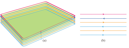
Figure 1: The bulk described by ACS action has a natural Luttinger liquid(s) boundary. (a) The bulk and boundary of one example with K matrix $K=\sigma_{z}\oplus\sigma_{x}\oplus\sigma_{x}$; (b) the non-chiral Luttinger liquid boundary has six edge fields, three propogating in clockwise and the other three anticlockwise.

The topological order described by Abelian Chern-Simons theory hosts Abelian anyon excitations. An anyon can be labeled by an integer vector $l=(l_{1},l_{2},...,l_{n})$. The self statistics of an anyon $l$ is given by

$$\theta_{l}=\pi l^{T}\cdot K^{-1}\cdot l$$ (2)

and the mutual statistics of two anyons $l$ and $l^{\prime}$ is given by

$$\theta_{l,l^{\prime}}=2\pi l^{T}\cdot K^{-1}\cdot l^{\prime}.$$ (3)

A bosonic excitation means that the self statistics is multiple of $2\pi$ while a fermion means that the self statistics is $\pi$ modular $2\pi$. The total number of anyons and the ground state degeneracy on torus are both given by $|\det{K}|$. In SPT phases, there is no anyons and the ground state is non-degenerate on any closed manifold, so we should require that $|\det(K)|=1$. In our later discussions, we will consider the presence of additional global symmetries. An external global $U(1)$ symmetry can be described by a charge vector by $q$. Then, the charge carried by an anyon excitation $l$ is

$$Q=q^{T}\cdot K^{-1}\cdot l$$ (4)

We note that readers shall not be confused with the $U(1)$ gauge symmetries of $a^{I}$ and the global $U(1)$ symmetry.

The K matrix Chern-Simons theory admits a well-known edge-bulk correspondence (see Fig.1) In a system with open boundary, the edge theory corresponding to (1) can take the form

$$\mathcal{L}_{edge}=\frac{K_{IJ}}{2\pi}\partial_{x}\phi_{I}\partial_{t}\phi_{J}+v_{IJ}\partial_{x}\phi_{I}\partial_{x}\phi_{J}+...$$ (5)

where $\phi_{I}$ is the chiral bosonic field on the edge and related to the bulk dynamical gauge field by $a_{\mu}^{I}=\partial_{\mu}\phi_{I}$. An anyon labeled by $l$ on the edge can be created by $e^{il^{T}\cdot\phi}$ where $\phi=(\phi_{1},\phi_{2},...,\phi_{n})$.

II.2 Symmetry implementation

II.2.1 Definition of symmetry in fSPT

Any fermionic system has the fermionic parity invariance. Namely, if we denote the total symmetry of an fSPT by $G_{f}$, then the fermion parity symmetry $\mathbb{Z}_{2}^{f}=\{1,P_{f}\}$ has to be a normal subgroup of $G_{f}$. The quotient group $G_{b}=G_{f}/\mathbb{Z}_{2}^{f}$ is the bosonic part of symmetry in the fSPT. Therefore, $G_{f}$ is a central extension of $G_{b}$ by $\mathbb{Z}_{2}^{f}$ which is labeled by the second group cohomology $\omega_{2}\in H^{2}(G_{b},\mathbb{Z}_{2}^{f})$. More precisely, $G_{f}$ defines as

$$0\longrightarrow\mathbb{Z}_{2}^{f}\longrightarrow G_{f}\longrightarrow G_{b}\longrightarrow 0$$ (6)

If the extension is trivial, $G_{f}=G_{b}\times\mathbb{Z}_{2}^{f}$, otherwise we denote $G_{f}=G_{b}\times_{\omega_{2}}\mathbb{Z}_{2}^{f}$. Note that the trivial element in $G_{b}$, which we denote as $e$, can be represented by $1$ or $P_{f}$. For example, since $H^{2}(\mathbb{Z}_{2},\mathbb{Z}_{2}^{f})=\mathbb{Z}_{2}$, there are two extensions of $G_{b}$. The trivial one is just $G_{b}=\mathbb{Z}_{2}\times\mathbb{Z}_{2}^{f}$ with two order-2 generators while the nontrivial one is $G_{f}=\mathbb{Z}_{2}\times_{\omega_{2}}\mathbb{Z}_{2}^{f}=\mathbb{Z}_{4}^{f}$ whose generator $g$ is order-4 and squares to $P_{f}$. Through out this paper, we focus on the Abelian $G_{f}$.

II.2.2 Implementing symmetry on the edge

We now consider how a symmetry is implemented in the edge theory. Under a symmetry operation $g$, the edge field $\phi_{I}$ transform as

$$g:\phi_{I}(x)\rightarrow W_{IJ}^{g}\phi_{J}(x)+\delta\phi^{g}_{I}$$ (7)

where the repeated $J$ is summed over and $W^{g}$ is an integral unimodular matrix such that

$$K=\eta_{g}(W^{g})^{T}KW^{g}$$ (8)

where $\eta_{g}=\pm$ corresponding to unitary $g$ or anti-unitary $g$. $\delta\phi^{g}$ is a constant vector up to $2\pi$. Accordingly, the excitation on the edge created by $e^{il^{T}\cdot\phi(x)}$ transform as

$$g:e^{il^{T}\cdot\phi(x)}\rightarrow e^{il^{T}\cdot W\cdot\phi(x)}e^{il^{T}\cdot\delta\phi^{g}}$$ (9)

The quantities $W^{g}$ and $\delta\phi^{g}$ in the transformation (7) can not be arbitrary. Besides (8), another natural constraint is that they should be compatible with the group structure of $G_{f}$. Specially, let us take $\{g_{1},g_{2},..,g_{k}\}$ to be the generators of a finite symmetry group. They satisfy a set of group relations in the following form

$$\prod_{i}^{k}g_{i}^{n_{i}}=1$$ (10)

where $n_{i}$ are integer. Then, acting both sides of (22) on the edge fields according to (7), we will require that

$$\prod_{i}^{k}g_{i}^{n_{i}}:\phi\rightarrow\phi\quad\text{ mod}\quad 2\pi$$ (11)

This set of conditions constrain possible values that $W^{g}$ and $\phi^{g}$ can take.

However, among the solutions $\{W^{g_{i}},\delta\phi^{g_{i}}\}$ of the above conditions, there is some redundancy. Two solutions related by the following gauge transformation are treated equivalently:

$$\tilde{W}^{g_{i}}=U^{-1}W^{g_{i}}U,$$ (12a)

$$\delta\tilde{\phi}^{g_{i}}=U^{-1}[\delta\phi^{g_{i}}-(1-\eta_{g_{i}}W^{g_{i}})\Delta\phi]$$ (12b)

where $U$ is a $n\times n$ integral unimodular matrix such that $U^{T}KU=K$ and $\Delta\phi$ is a constant vector up to $2\pi$ and $\eta_{g}=\pm$ denotes the group element $g$ to be unitary/anti-unitary.

Thoughout this paper, we use the notation of $[K,\{W^{g_{i}},\delta\phi^{g_{i}}\}]$ to denote a consistent realization of a certain symmetry in the bulk and also on the edge whose low energy physics are described by ACS theory with K matrix $K$ and its canonical Luttinger liquid edge theory. The consistency is guaranteed by that it is a solution for constraint equations enforced by symmetry. Below we call $[K,\{W^{g_{i}},\delta\phi^{g_{i}}\}]$ as state, phase or solution interchangeably. Without causing confusion, we sometimes omit $K$ matrix and only list the realization of generator(s) of symmetry group in the notation $[K,\{W^{g_{i}},\delta\phi^{g_{i}}\}]$.

II.2.3 Fermion parity operator

Since every fSPT is invariant under the fermion parity, here we pay special attention to the fermion parity operator. It is well-known that any $2\times 2$ K matrix for fSPT can transform into $\sigma_{z}$ via proper modular transformation. Then, for $K=\sigma_{z}$, the fermion parity should realize as[57]

$$W^{P_{f}}=1_{2\times 2},\quad\delta\phi^{P_{f}}=\pi\begin{pmatrix}1\\ 1\end{pmatrix}.$$ (13)

To justify it, we consider two basic facts: (1) two basic fermionic excitations $e^{i\phi_{1}},e^{i\phi_{2}}$ aquire a minus sign under the fermion parity, and any bosonic excitation $e^{i(l_{1}\phi_{1}+l_{2}\phi_{2})}$ with $l_{1}+l_{2}=0$ mod 2 is invariant under fermion parity, (2) with only $\mathbb{Z}_{2}^{f}$ symmetry, any bosonic excitation can condense to gap out the edge modes without breaking any symmetry.

In the following, most of our examples are with $K=\sigma_{z}$, and we always assume the fermion parity is realized as (13). For those with larger dimensional $K$ matrix in this paper, $K$ would take the form as $\sigma_{z}\oplus\sigma_{x}\oplus...\oplus\sigma_{x}$, then the fermion parity is simply generalized into the form

$$W^{P_{f}}=1_{2\times 2}\oplus 1_{2\times 2}\oplus...\oplus 1_{2\times 2},$$ (14)

$$\quad\delta\phi^{P_{f}}=\pi\begin{pmatrix}1\\ 1\end{pmatrix}\oplus\begin{pmatrix}0\\ 0\end{pmatrix}\oplus...\oplus\begin{pmatrix}0\\ 0\end{pmatrix}.$$ (15)

II.3 Stacking of SPT phases

For two fSPT phases described by two ACS theories $[K,\{W^{g_{i}},\delta\phi^{g_{i}}\}]$ and $[\tilde{K},\{\tilde{W}^{g_{i}},\delta\tilde{\phi}^{g_{i}}\}]$, the stacking of these two phases forms a new phase, which is described by a new ACS theory $[K_{s}=K\oplus\tilde{K},\{W_{s}^{g_{i}}=W^{g_{i}}\oplus\tilde{W}^{g_{i}},\delta\phi^{g_{i}}_{s}=\delta\phi^{g_{i}}\oplus\delta\tilde{\phi}^{g_{i}}\}]$. If the classificaion of fSPT is an Abelian group, then the stacking operation is the group operation of the classification group. We also use the notation $[K,\{W^{g_{i}},\delta\phi^{g_{i}}\}]^{-1}$ as the inverse phase of $[K,\{W^{g_{i}},\delta\phi^{g_{i}}\}]$ in the classification group. The stacking operation can also be well-defined for many phases. In particular, we might use the notation $[K,\{W^{g_{i}},\delta\phi^{g_{i}}\}]^{\oplus n}$ as phase that is a stacking of $n$-copy phases of $[K,\{W^{g_{i}},\delta\phi^{g_{i}}\}]$.

For example, the classification $\mathbb{Z}_{2}^{f}\times\mathbb{Z}_{2}$ fSPT is $\mathbb{Z}_{8}$ whose generator is denoted by $w$, if the root phase labeled by $w$ can be realized by an ACS theory with $[K_{1},\{W_{1}^{g_{i}},\delta\phi_{1}^{g_{i}}\}]$, then two copies of $w$ stack to a new phase labeled by $w^{2}$ and similarly eight copies stack to $w^{8}=1$ which is trivial and hence whose edge can be symmetrically gapped out. The root state can also be realized by another ACS theory with $[K^{\prime}_{1},\{{W^{\prime}}_{1}^{g_{i}},\delta{\phi^{\prime}}_{1}^{g_{i}}\}]$, then the stacking theory $[K_{2}=K_{1}\oplus K_{1}^{\prime},\{W_{2}^{g_{i}}=W_{1}^{g_{i}}\oplus{W^{\prime}}_{1}^{g_{i}},\delta\phi_{2}^{g_{i}}=\delta{\phi}_{1}^{g_{i}}\oplus\delta{\phi^{\prime}}_{1}^{g_{i}}\}]$ also describes a phase labeled by $w^{2}$.

II.4 Detecting the symmetry anomaly on the boundary

Here we discuss two different ways to dectect whether the symmetry on boundary is anomalous or not. The first one, as discuss in Sec.II.4.1, directly studies the stability of the edge fields, while the second one, in Sec.II.4.2, turns to study the the topological properties of symmetry flux that can characterize SPT phase (see Fig.2). In practice, the first one is convenient for proving a phase is trivial since the symmetric Higgs terms for symmetrically and fully gapping out the edge fields may be easily constructed, while the latter may be especially useful to assert that a phase is nontrivial and also assert which nontrivial phase it belongs to.

II.4.1 Ingappability without breaking symmetry

The nontrivial topology of nontrivial SPT phases can be manifest on their boundaries where the symmetry is anomalous. The existence of symmetry anomaly on the boundary is in fact one defining property of SPT phases and has direct physical consequence that the boundary can not be adiabatically connected to symmetric short range entangled states. In general, the boundary of nontrivial SPT can only be gapless, spontaneously symmetry breaking or develop topological order if not breaking symmetry. For 2D nontrivial SPT, as there is no nontrivial topological order in 1D, their 1D edges can only be gapless without breaking symmetry or gapped with breaking symmetry.

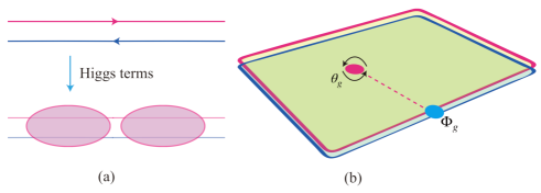
Figure 2: Two approaches to detect the symmetry anomaly. (a) If there exist symmetric Higgs term(s) that can drive the edge Luttinger liquid to a symmetric short range entangled state, the bulk is a trivial SPT; otherwise, it is nontrivial SPT. (b) The symmetric flux are inserted, whose topological spin or (projective) representation of other symmetry can be used to detect whether a SPT is nontrivial or not. If the symmetry $g$ does not permute edge fields, but only shift them by a phase shift $\delta\phi^{g}$, the symmetry defect on the boundary can be created by applying the “frationalized” operator $\Phi_{\text{g}}=e^{iK^{-1}\cdot\delta\phi^{g}\cdot\phi}$.

Based on the properties, we can detect whether a SPT phase is nontrivial or not by studying the stability of its edge modes. If its edge modes can be symmetrically fully gapped out, then it must be a trivial SPT, otherwise, it is a nontrivial one. We can call this criterion as ingappability criterion. In particular, for the SPT phases realized by $K$ matrix ACS theories, we have the following two pratical ways to see whether they are nontrivial or not based on the ingappibility criterion.

The first one is the so-called null-vector criterion that is directly related to the bosonic edge fields. To symmetrically gap out the bosonic edge fields (5), we can condense some bosons, namely by adding the Higgs terms

$$\mathcal{L}_{hig}=\sum_{i}C_{i}\cos(l_{i}^{T}\cdot\phi+\alpha_{i})$$ (16)

The perturbative terms should satisfy the following conditions. First, it should be symmetric under every symmetry, $g:\mathcal{L}_{hig}\rightarrow\mathcal{L}_{hig}$. Second, for a $2n\times 2n$ K matrix, it needs $n$ different Higgs terms with vectors $l_{1,2,...,n}$ to fully gap out the edge. The $n$ vectors $l_{1},l_{2},\dots,l_{n}$ should be linearly independent. Third, the Higgs terms should satisfy the so-called null-vector condition. To illustrate it, we construct $n$ different integer vectors $\Lambda_{i}:=K^{-1}\cdot l_{i}$. The null vector condition then states that the corresponding edge theory can be fully gapped out if and only if the following conditions are satisfied

$$\Lambda_{i}^{T}K\Lambda_{i}=0\,\text{ for all\text{ }}i$$ (17)

$$\Lambda_{i}^{T}K\Lambda_{j}=0\,\text{ for\, all\, pairs\, of }\,i,j$$ (18)

Fourth, it is required that no spontaneously symmetry breaking occurs, once the edge fields are fully gapped by $\mathcal{L}_{hig}$. For this, it is required that the greatest common divisor of all the $n\times n$ minors of the matrix $(\Lambda_{1},\Lambda_{2},...,\Lambda_{n})$ is $\pm 1$.

If the Higgs terms satisfying the above conditions exist, the edge can be fully gapped without breaking any symmetry. Then, the symmetry realization in the edge theory is anomaly-free. This means the bulk fSPT is trivial. Otherwise, if the edge modes can not be symmetrically gapped out, it means the symmetry realization is anomalous, which indicates the bulk fSPT is non-trivial.

The second one utilizes the so-called refermionization of the scalar bosonic edge fields (5). For many cases, the K matrix we study takes the form as $K=(\sigma_{z})^{\oplus n}$, whose edge fields are denoted $\phi_{i},i=1,2,...,2n$. We can define $2n$ fermions by $\psi_{i}\sim e^{i\phi_{i}}$ and transform the edge theory (5) in terms of bosonic edge fields with certain radius into an edge theory in terms of fermionic fields. Then the staibility of this fermionic edge theory can be studied by checking whether there is symmetric mass (interaction) term to gap out the edge fields. As in many examples as follows, transforming the bosonic edge field theories into a fermionic one may be more simpler to find the symmetric mass terms to fully gap out the edge fields.

We stress that the above two ways are not totally different from each other. In fact, they are equivalent in certain cases. However, we illustrate them here explicitly just for pratical purpose.

II.4.2 Symmetry flux

Whether the symmetry realization is anomalous or not can also be checked by the properties of symmetry fluxes. Here, we consider two examples for illustration. First let us consider $\mathbb{Z}_{N}$ symmetry group for examples. One possible realization of the generator $g_{1}$ of $\mathbb{Z}_{N}$ group is

$$W^{g_{1}}=1,\quad\delta\phi^{g_{1}}=\frac{2\pi}{N}K^{-1}\cdot\chi_{g_{1}}$$ (19)

where $\chi_{g_{1}}$ is an integer vector. $K$ is the K matrix for SPT phase. The phase shift $\delta\phi^{g_{1}}$ has a physical meaning, that is the symmetry charge carried by the excitation created by $e^{i\phi}$. More precisly, we can denote the charge vector of the $n$ different fundamental excitations $e^{i\phi_{i}}$ by $q=\chi_{g_{1}}$. Therefore, via (4), the symmetry charge of the excitation labeled by $l$ is $Q=q^{T}\cdot K^{-1}\cdot l$, if we view $\mathbb{Z}_{N}$ as a subgroup of $U(1)$. Now we consider inserting the elementary symmetry flux $\frac{2\pi}{N}$ in the system, and the Berry phase accumulated when braiding the excitation $l$ around this symmetry flux is simply given by

$$\theta_{g,l}=\frac{2\pi}{N}Q=2\pi\frac{\chi_{g_{1}}^{T}}{N}\cdot K^{-1}\cdot l$$ (20)

Compared with (3), the effective label of the symmetry flux in this K matrix framework is $l=\frac{\chi_{g_{1}}}{N}$ which means that the “fractionalized” vertex operator $e^{i\frac{1}{N}\chi^{T}_{g_{1}}\cdot\phi}$ can be treated as the symmetry flux of this $Z_{N}$ symmetry with the same $K$ matrix (see.Fig.2). There actually is no such kind of fractionalized dynamical excitations in the SPT bulk. Since by inserting symmetry flux in the system, we have to create an branch cut which is singular, we understand that this “fractionalized excitation” is actually a static defect which lies at the end of the branch cut. Nevertheless, we can continue to calculate the “topological spin” of the symmetry flux as

$$\theta_{g_{1}}=\frac{\pi}{N^{2}}\chi_{g_{1}}^{T}\cdot K^{-1}\cdot\chi_{g_{1}}$$ (21)

which would become the true value of topological spin of gauge flux once we gauge this symmetry. If the edge can be gapped out without breaking the symmetry, it is required that $N\theta_{g_{1}}=0$ modulo $2\pi$. If this condition is satisfied, it means that there exists a bosonic symmetry flux and then we can condense it without breaking the symmetry. This physical intuitive understanding can be refered to more rigorous derivation in Ref.[19].

Let us consider another example. For the non-Abelian root state protected by $(\mathbb{Z}_{N})^{3}$ symmetry, a sufficient property is that the symmetry flux corresponding to one $\mathbb{Z}_{N}$ subgroup carries the fundamental projective representation of the rest $\mathbb{Z}_{N}\times\mathbb{Z}_{N}$ subgroup. Supposed one of the $\mathbb{Z}_{N}$ symmetry subgroup realizes as (19), ad the other two are realized as, generally speaking, $\{W^{g_{2}},\delta\phi^{g_{2}}\}$ and $\{W^{g_{3}},\delta\phi^{g_{3}}\}$ where $g_{2}$ and $g_{3}$ are the two generators of the rest two $\mathbb{Z}_{N}$ subgroups. Then acting on the symmetry flux related to the first $\mathbb{Z}_{N}$ subgroup, the representative matrices of $g_{2}$ and $g_{3}$ should form the fundamental projective representation of $\mathbb{Z}_{N}\times\mathbb{Z}_{N}$ group[55].

II.5 Main Results

In this section, we will present our main results: we aim to find out the edge theories for various fSPT in the K matrix formulism. The root phase results are summarized in Table.1. Here we briefly summarized the results we obtain. In the following, for most cases, we take the K matrix as $K=\sigma_{z}$. So if there is no claim on the explicit form of K matrix, it is assumed that $K=\sigma_{z}$.

1. $\mathbb{Z}_{2}\times\mathbb{Z}_{2}^{f}:$ The classification of fSPT protected by this symmetry is $\mathbb{Z}_{8}$. The root phase is identified as that with $W^{g}=\sigma_{z},\delta\phi^{g}=0$. The physics of this root phase is that the edge hold two gapless majorana fermions that propogate in opposite directions. We note that the majorana fermion edge theory for SET emerged from ACS theory is also discussed in Ref.[59] and for $\mathbb{Z}_{2}\times\mathbb{Z}_{2}^{f}$ SPT in Ref.[58]. However we discuss more thoroughly here, including how other phases are related to each other, as see the phase relation (35)-(40).

2. $\mathbb{Z}_{4}\times\mathbb{Z}_{2}^{f}:$ The classification of fSPT protected by this symmetry is $\mathbb{Z}_{8}\times\mathbb{Z}_{2}$, we find that the root phase for the $\mathbb{Z}_{8}$ classification is the phase with $W^{g}=1_{2\times 2}$, $\delta\phi^{g}=(0,{\pi}/{2})^{T}$. In this case, the edge fields when being gapless is a $c=1$ Luttinger liquid. The root phase for $\mathbb{Z}_{2}$ classification is identified by the phase with $K=(\sigma_{z})^{\oplus 3}$ and $W^{g}=\sigma_{z}\oplus(1_{2\times 2})^{\oplus 2},\delta\phi^{g}=(0,0)^{T}\oplus(0,\pi/2)^{T}\oplus(0,\pi/2)^{T}$. This root phase in fact is a stacking phase that consists of the phase with $K=\sigma_{z}$ and $W^{g}=\sigma_{z},\delta\phi^{g}=0$ and two copies of that above $\mathbb{Z}_{8}$ root phase, which admits odd number of gapless majorana fermions on the edge.

   Besides these two root phases, there are also many other allowed states. We also show that the relations between other phases and the root ones, such as (65c)-(66f).

3. $\mathbb{Z}_{2}\times\mathbb{Z}_{2}\times\mathbb{Z}_{2}^{f}:$ The classification of this symmetry is $\mathbb{Z}_{8}\times\mathbb{Z}_{8}\times\mathbb{Z}_{4}$, hence there are three root phases, two of which are just the ones that protected by a single $\mathbb{Z}_{2}$ subgroup alone, which are easily obtained by choosing the other $\mathbb{Z}_{2}$ subgroup being totally trivial. These two root states are just the ones with odd number of gapless majorana fermions.

   The third root phase is identified to the one with $W^{g_{1}}=W^{g_{2}}=-1_{2\times 2},\delta\phi^{g_{1}}=(0,\pi),\delta\phi^{g_{2}}=0$. We note that the fermion parity is to realize as $W^{P_{f}}=1_{2\times 2},\delta\phi^{P_{f}}=(\pi,\pi)^{T}$. We find that this root phase can be trivialized by four copies of them, but not by two copies, hence it is not a $\mathbb{Z}_{2}$ root phase. We also find that when acting on the symmetry flux labeled by $g_{1}$, the $\mathbb{Z}_{2}\times\mathbb{Z}_{2}^{f}$ form the projective representation, which indicates that the root phase is a ferminic non-Abelian SET upon gauging the whole symmetry.

   There are various other allowed states, in addition to these three root ones, whose relations to the roots ones are also obtained in Sec.III.3.4 and also in Appendix.A.

4. $\mathbb{Z}_{8}^{f}:$ The classification of fSPT protected by this symmetry is $\mathbb{Z}_{2}$. The root phase is identified as the one with $W^{g}=1_{2\times 2},\delta\phi^{g}=(\pi/4,3\pi/4)$. We find that to see that two copies of this root state is indeed trivial; a easy way is to stack them with additional two trivial phases. Compared to the $\mathbb{Z}_{4}\times\mathbb{Z}_{2}^{f}$ symmetry where $\mathbb{Z}_{4}$ is trivial extension of $\mathbb{Z}_{2}^{f}$, we find that due to the presence of nontrivial $\mathbb{Z}_{2}^{f}$ extension, the symmetry transformations as $W^{g}=\pm\sigma_{z},-1$ are not consistent with the symmetry, which indicates that the edge with odd number of gapless majorana fermion are not consistent in this case. We also discuss typical phases relations, such as (112)-(114) between the root and other allowed states.

5. $\mathbb{Z}_{2}\times\mathbb{Z}_{4}^{f}:$ The classification of this symmetry $\mathbb{Z}_{4}$. The root state is identified as the one with $W^{g_{1}}=W^{g_{2}}=1_{2\times 2},\delta\phi^{g_{1}}=(0,\pi),\delta\phi^{g_{2}}=(\pi/2,\pi/2)$. Similarly to $\mathbb{Z}_{8}^{f}$, the realizations of symmetry $\mathbb{Z}_{2}\times\mathbb{Z}_{2}\times\mathbb{Z}_{2}^{f}$ with $W^{g_{1}}=\pm\sigma_{z}$ or $W^{g_{2}}=\pm\sigma_{z}$ which give rise to the edge with odd number of gapless majorana fermion are not consistent in this case. We also discuss typical phases relations, such as (122a)-(122c), between the root and other allowed states.

6. $\mathbb{Z}_{4}\times\mathbb{Z}_{4}^{f}$: The classification of this symmetry $\mathbb{Z}_{8}\times\mathbb{Z}_{2}$. The root state for the $\mathbb{Z}_{2}$ classification is identified as the one with $W^{g_{1}}=W^{g_{2}}=1_{2\times 2}$ and $\delta\phi^{g_{1}}=(\pi/2,-\pi/2),\delta\phi^{g_{2}}=(\pi/2,\pi/2)$, while the one for the $\mathbb{Z}_{8}$ classification is with $W^{g_{1}}=W^{g_{2}}=1_{2\times 2}$ and $\delta\phi^{g_{1}}=(\pi/2,\pi/2),\delta\phi^{g_{2}}=(0,\pi/2)$. One way to see that they are indeed different root states is to see the “topological spin” of symmetry flux $g_{2}$, which is $0$ for the former one and $\frac{\pi}{16}$ for the latter. We also discuss the relations between other states and the two root ones, as (132a)-(132c).

7. $G_{b}=\mathbb{Z}_{n}\times\mathbb{Z}_{n}\times\mathbb{Z}_{n}:$ We find the symmetry realization with the Type-III anomaly on the edge fields of the root state. One way to detect whether the symmetry realization on the edges is with Type-III anomaly is to check whether one of the symmetry flux carries the projective representation of the left subgroup. We come up with a construction of the realization of the Type-III anomaly of root phases protected by $(\mathbb{Z}_{n})^{3}$ with central charge $c=n-1$, and illustrating that by the examples of $n=2,3,4,5$ explicitly.

8. $G_{f}=\mathbb{Z}_{4}^{f}\times\mathbb{Z}_{4}\times\mathbb{Z}_{4}:$ We construct the edge theory of the intrinsically interacting fSPT root phase that can also be realized with central charge $c=3$. Fingerprint of this root phase is that the $\frac{\pi}{2}$ flux defect of $\mathbb{Z}_{4}^{f}$ carries the fundamental projective representation of the other $\mathbb{Z}_{4}\times\mathbb{Z}_{4}$ symmetry. We also argue that phase with two these root phase stacking is equivalent to the Type-III nontrivial bSPT protected by $\mathbb{Z}_{2}\times\mathbb{Z}_{4}\times\mathbb{Z}_{4}$ symmetry. In this sense, we can call that the root state of intrinsically interacting fSPT of $\mathbb{Z}_{4}^{f}\times\mathbb{Z}_{4}\times\mathbb{Z}_{4}$ is the square root of the Type-III nontrivial bSPT protected by $\mathbb{Z}_{2}\times\mathbb{Z}_{4}\times\mathbb{Z}_{4}$ symmetry.

Symmetry	Classification	Generators	K matrix and symmetry transformation	note
$\mathbb{Z}_{8}^{f}$	$\mathbb{Z}_{2}$	$g$	$K=\sigma_{z}$, $W^{g}=1_{2\times 2},\delta\phi^{g}=\frac{\pi}{4}$ $\begin{pmatrix}1\\ -1\end{pmatrix}$
$\mathbb{Z}_{2}\times\mathbb{Z}_{2}^{f}$	$\mathbb{Z}_{8}$	$g$	$K=\sigma_{z}$, $W^{g}=\sigma_{z},\delta\phi^{g}=0$
$\mathbb{Z}_{4}\times\mathbb{Z}_{2}^{f}$	$\mathbb{Z}_{8}\times\mathbb{Z}_{2}$	$(g,P_{f})$	$root$ $1$: $K=\sigma_{z}$, $W^{g}=1_{2\times 2},$ $\delta\phi^{g}=\frac{\pi}{2}\begin{pmatrix}0\\ 1\end{pmatrix}$
			$root$ $2$: $K=\sigma_{z}^{\oplus 3}$, $W^{g}=\sigma_{z}\oplus 1_{4\times 4},\delta\phi^{g}=\frac{\pi}{2}\begin{pmatrix}0\\ 0\end{pmatrix}\oplus\begin{pmatrix}0\\ 1\end{pmatrix}\oplus\begin{pmatrix}0\\ 1\end{pmatrix}$
$\mathbb{Z}_{2}\times\mathbb{Z}_{4}^{f}$	$\mathbb{Z}_{4}$	$(g_{1},g_{2})$	$K=\sigma_{z}$, $W^{g_{1}}=W^{g_{2}}=1_{2\times 2},\delta\phi^{g_{1}}=\pi\begin{pmatrix}0\\ 1\end{pmatrix},\delta\phi^{g_{2}}=\frac{\pi}{2}\begin{pmatrix}1\\ 1\end{pmatrix}$
$\mathbb{Z}_{4}\times\mathbb{Z}_{4}^{f}$	$\mathbb{Z}_{2}\times\mathbb{Z}_{8}$	$(g_{1},g_{2})$	$root$ $1:$ $K=\sigma_{z},W^{g_{1,2}}=1_{2\times 2},\delta\phi^{g_{1}}=\frac{\pi}{2}\begin{pmatrix}1\\ -1\end{pmatrix},\delta\phi^{g_{2}}=\frac{\pi}{2}\begin{pmatrix}1\\ 1\end{pmatrix}$
			$root$ $2:$ $K=\sigma_{z}$, $W^{g_{1,2}}=1_{2\times 2},\delta\phi^{g_{1}}=\frac{\pi}{2}\begin{pmatrix}1\\ 1\end{pmatrix},\delta\phi^{g_{2}}=\frac{\pi}{2}\begin{pmatrix}0\\ 1\end{pmatrix}$
$\mathbb{Z}_{2}\times\mathbb{Z}_{2}\times\mathbb{Z}_{2}^{f}$	$(\mathbb{Z}_{8})^{2}\times\mathbb{Z}_{4}$	$(g_{1},g_{2},P_{f})$	$root\,1:$ $K=\sigma_{z},W^{g_{1}}=\sigma_{z},W^{g_{2}}=1_{2\times 2},\delta\phi^{g_{1}}=0,\delta\phi^{g_{2}}=0$
			$root\,2:$ $K=\sigma_{z},W^{g_{1}}=1_{2\times 2},W^{g_{2}}=\sigma_{z},\delta\phi^{g_{1}}=0,\delta\phi^{g_{2}}=0$
			$root\,3:$ $K=\sigma_{z},W^{g_{1}}=W^{g_{2}}=-1_{2\times 2},\delta\phi^{g_{1}}=\pi\begin{pmatrix}0\\ 1\end{pmatrix},\delta\phi^{g_{2}}=0$
			$type$-$III$ $root$ : $K=\sigma_{x},W^{g_{1}}=-W^{g_{2}}=-W^{g_{3}}=1_{2\times 2},$
$\mathbb{Z}_{2}\times\mathbb{Z}_{2}\times\mathbb{Z}_{2}$	$type$-$III:$	$(g_{1},g_{2},g_{3})$
	$\mathbb{Z}_{2}$		$\delta\phi^{g_{1}}=\pi\begin{pmatrix}1\\ 0\end{pmatrix},\delta\phi^{g_{2}}=0,\delta\phi^{g_{3}}=\pi\begin{pmatrix}0\\ 1\end{pmatrix}$	(below we denote $-i$ by $\bar{i}$)
			$type$-$III$ $root$ : $K=(\sigma_{x})^{\oplus 2},W^{g_{1}}=1_{4\times 4},W^{g_{2}}=A_{3},$
$\mathbb{Z}_{3}\times\mathbb{Z}_{3}\times\mathbb{Z}_{3}$	$type$-$III$:	$(g_{1},g_{2},g_{3})$		$A_{3}=\begin{pmatrix}0&0&\bar{1}&0\\ 0&\bar{1}&0&\bar{1}\\ {1}&0&\bar{1}&0\\ 0&{1}&0&0\end{pmatrix}$
	$\mathbb{Z}_{3}$		$W^{g_{3}}=(A_{3})^{2},\delta\phi^{g_{1}}=\frac{2\pi}{3}\begin{pmatrix}{1}\\ 0\\ {-1}\\ 0\end{pmatrix},\delta\phi^{g_{2}}=0,\delta\phi^{g_{3}}=\frac{\pi}{3}\begin{pmatrix}0\\ 1\\ 0\\ 1\end{pmatrix}$
			$type$-$III$ $root$ : $K=(\sigma_{x})^{\oplus 3},W^{g_{1}}=1_{6\times 6},W^{g_{2}}=A_{4},$
$\mathbb{Z}_{4}\times\mathbb{Z}_{4}\times\mathbb{Z}_{4}$	$type$-$III:$	$(g_{1},g_{2},g_{3})$		$A_{4}=\begin{pmatrix}0&0&\bar{1}&0&0&0\\ 0&\bar{1}&0&\bar{1}&\bar{1}&0\\ 0&0&\bar{1}&0&0&{1}\\ 0&0&0&0&1&0\\ 0&{1}&0&0&0&0\\ 1&0&\bar{1}&0&0&0\end{pmatrix}$
	$\mathbb{Z}_{4}$		$W^{g_{3}}=(A_{4})^{3},\delta\phi^{g_{1}}=\frac{\pi}{2}{\begin{pmatrix}1\\ 0\\ -1\\ 0\\ 0\\ 2\end{pmatrix}},\delta\phi^{g_{2}}=0,\delta\phi^{g_{3}}=\frac{\pi}{2}{\begin{pmatrix}0\\ 1\\ 0\\ 1\\ 1\\ 0\end{pmatrix}}$
			$type$-$III$ $root$ : $K=(\sigma_{x})^{\oplus 4},W^{g_{1}}=1_{8\times 8},W^{g_{2}}=A_{5},$
$\mathbb{Z}_{5}\times\mathbb{Z}_{5}\times\mathbb{Z}_{5}$	$type$-$III:$	$(g_{1},g_{2},g_{3})$		$A_{5}=\begin{pmatrix}0&0&0&1&\bar{1}&0&0&0\\ 0&0&1&0&0&0&0&0\\ 0&0&0&0&0&0&1&0\\ 0&0&0&0&\bar{1}&0&0&1\\ 1&0&0&0&\bar{1}&0&0&0\\ 0&1&0&0&0&0&0&0\\ 0&\bar{1}&\bar{1}&0&0&\bar{1}&\bar{1}&0\\ 0&0&0&0&\bar{1}&0&0&0\end{pmatrix}$
	$\mathbb{Z}_{5}$		$W^{g_{3}}=(A_{5})^{4},\delta\phi^{g_{1}}=\frac{2\pi}{5}\begin{pmatrix}3\\ 0\\ 0\\ 2\\ -1\\ 0\\ 0\\ 1\end{pmatrix},\delta\phi^{g_{2}}=0,\delta\phi^{g_{3}}=\frac{2\pi}{5}\begin{pmatrix}0\\ 1\\ 1\\ 0\\ 0\\ 1\\ 1\\ 0\end{pmatrix}$
			$intrinsic$ $root$ : $K=\sigma_{z}\oplus(\sigma_{x})^{\oplus 2},W^{g_{1}}=1_{6\times 6},W^{g_{2}}=\tilde{A}_{4},$
$\mathbb{Z}_{4}^{f}\times\mathbb{Z}_{4}\times\mathbb{Z}_{4}$	$intrinsic$	$(g_{1},g_{2},g_{3})$		$\tilde{A}_{4}=\left(\begin{array}[]{cccccc}1&0&0&\bar{2}&0&\bar{1}\\ 0&1&0&2&0&\bar{1}\\ 0&0&0&0&0&1\\ 1&\bar{1}&0&\bar{2}&1&0\\ 0&0&0&1&0&0\\ 2&2&1&0&0&\bar{2}\\ \end{array}\right)$
	$\mathbb{Z}_{4}$		$W^{g_{3}}=(\tilde{A}_{4})^{3},\delta\phi^{g_{1}}=\frac{\pi}{2}{\begin{pmatrix}1\\ 1\\ 0\\ 0\\ 0\\ 0\end{pmatrix}},\delta\phi^{g_{2}}=0,\delta\phi^{g_{3}}=\frac{\pi}{2}{\begin{pmatrix}2\\ 0\\ 2\\ 1\\ 1\\ 2\end{pmatrix}}$

Table 1: Symmetry transformation on edge fields of fSPT root state. For some $G_{f}$ symmetry, we list all their root states while for $G_{b}=(\mathbb{Z}_{n})^{3}$, we only list the root state of type-III bosonic SPT which can not be trivialized in fermionic system. For $G_{f}=\mathbb{Z}_{4}^{f}\times\mathbb{Z}_{4}\times\mathbb{Z}_{4}$, we only list the root state for the intrinsically interacting fSPT.

III $G_{b}\times\mathbb{Z}_{2}^{f}$ type of symmetry group

Here we consider the examples with $G_{f}=G_{b}\times\mathbb{Z}_{2}^{f}$. More specifically, we consider carefully three examples: $\mathbb{Z}_{2}\times\mathbb{Z}_{2}^{f}$, $\mathbb{Z}_{4}\times\mathbb{Z}_{2}^{f}$ and $\mathbb{Z}_{2}\times\mathbb{Z}_{2}\times\mathbb{Z}_{2}^{f}$ whose classifiations of SPT are $\mathbb{Z}_{8}$, $\mathbb{Z}_{8}\times\mathbb{Z}_{2}$ and $(\mathbb{Z}_{8})^{2}\times\mathbb{Z}_{2}$ respectively.

III.1 $\mathbb{Z}_{2}\times\mathbb{Z}_{2}^{f}$ symmetry

III.1.1 Symmetry realization

Here we figure out all possible symmetry realization with the simplest K matrix i.e., $K=\sigma_{z}$.

The generators of this symmetry group are denoted as $g$ and $P_{f}$ with the group relation as $g^{2}=1$ and $P_{f}^{2}=1$. As mentioned above, the parity realizes as (13) and the group relation of $g$ indicates

$$(W^{g})^{2}=1_{2\times 2}.$$ (22)

Therefore, taking into acount the constraint (8), $W^{g}$ can take $\pm 1_{2\times 2}$, $\pm\sigma_{z}$ and we have

$$W_{IJ}^{g}\delta\phi_{J}^{g}+\delta\phi_{I}^{g}=0.$$ (23)

where the repeated $J$ is summed. Note that $W^{g}$ and $\delta\phi^{g}$ consist the full implementation of symmetry action $g$ in this system. Below we will solve (23) for $\delta\phi^{g}$ with different $W^{g}$.

1. For $W^{g}=1_{2\times 2}$, via solving (23), we get $\delta\phi^{g}=\pi(t_{1},t_{2})^{T}$ with $t_{1},t_{2}=0,1$ and then we can denote the SPT phases correspongding to $t_{1},t_{2}$ by $[1_{2\times 2},t_{1},t_{2}]$.

2. For $W^{g}=-1$, the equation (23) does not impost any constraint on $\delta\phi^{g}$, therefore $\delta\phi^{g}=(\theta_{1},\theta_{2})^{T}$ with $\theta_{1,2}\in[0,2\pi)$. However, via the gauge transformation on $\phi$, we can get $\delta\phi^{g}=0$.

3. For $W^{g}=\sigma_{z}$, via solving (23), we get $\delta\phi^{g}=(n\pi,\theta)^{T}$ where $\theta\in[0,2\pi]$ and $n=0,1$. Using the gauge transformation, we can shift $\theta=0$. Therefore

   $$\delta\phi^{g}=\begin{pmatrix}n\pi\\ 0\end{pmatrix},\text{ }n=0,1$$ (24)

   We denote the phases related to $W^{g}=\sigma_{z}$ as $[\sigma_{z},n]$.

4. For $W^{g}=-\sigma_{z}$, via solving (23), we get $\delta\phi^{g}=(\theta,n\pi,)^{T}$ with $\theta\in[0,2\pi)$ and $n=0,1$. Using the gauge transformation, we can shift $\theta=0$. Therefore

   $$\delta\phi^{g}=\begin{pmatrix}0\\ n\pi\end{pmatrix},\text{ }n=0,1$$ (25)

   We denote the phases related to $W^{g}=\sigma_{z}$ as $[-\sigma_{z},n]$.

Below we will first show that symmetry realization corresponding to the root for classification and then discuss how phases related to other symmetry realizations relate to the root one.

III.1.2 Root phase

Here we show that the root phase is identified as the phase with $[\sigma_{z},0]$, namely $W^{g}=\sigma_{z}$ and $\delta\phi^{g}=0$.

The physics of the root phase is that its edge holds two robust counter-propagating gapless majorana fermion fields. For $[\sigma_{z},0]$, to obtain the gapless Majorana fermion edge from the Luttinger liquid edge theory (5), we consider the following symmetric Higgs terms

$$S_{edge}^{1}=\sum_{l}g_{l}\int dxdt\text{ cos}[l(\phi_{1}+\phi_{2})+\alpha_{l}]$$

$$+\text{cos}[l(\phi_{1}-\phi_{2})+\alpha_{l}]$$ (26)

The two Higgs terms with the same coupling constant is guaranteed by the symmetry action. Since $\phi_{1}+\phi_{2}$ and $\phi_{1}-\phi_{2}$ do not commute, they can not condense simutaneously. Naively, one might conclude that the edge modes $\phi_{1}$ and $\phi_{2}$ remain gapless Luttinger liquid state and propagate in opposite directions. However, things are not so disppointed. Due to the fact that the coupling constant are always the same for $\text{ cos}[l(\phi_{1}+\phi_{2})+\alpha_{l}]$ and $\text{cos}[l(\phi_{1}-\phi_{2})+\alpha_{l}]$, the nonzero $g_{l}$ can drive the Luttinger liquid to some other nontrivial universality class. For simplicity, we first consider the most relevant case $l=1$. Then the edge theory is

$$S_{edge}= \frac{1}{4\pi}\int dxdt(-1)^{i-1}\partial_{t}\phi_{i}\partial_{x}\phi_{i}+\partial_{x}\phi_{i}v_{ij}\partial_{x}\phi_{j}$$

$$+g_{1}\int dxdt\text{ cos}(\phi_{1}+\phi_{2})+\text{cos}(\phi_{1}-\phi_{2})$$ (27)

where the repeated $i,j$ are summed and $\alpha_{1}$ is absorbed. To be invariant under symmetry, $v_{12}=v_{21}=0$. Without affecting the symmetry anomaly, we tune $v_{11}=v_{22}=v$ for convenience. Under basis transformation $\phi_{1}=\phi+\theta$, $\phi_{2}=\phi-\theta$, the edge theory can be quantized to be

$$H=\frac{v}{2\pi}\int dx(\partial_{x}\phi)^{2}+(\partial_{x}\theta)^{2}$$

$$+g_{1}\int dx\text{ cos}(2\phi)+\text{cos}(2\theta).$$ (28)

It is well-known that these Higgs terms $g_{1}$ leads the system to lie at the Ising cricality. To see this, define majorana fermion $\eta_{R,L}^{1,2}$ by

$$\eta_{R}^{1}+i\eta_{R}^{2}=\frac{1}{\sqrt{\pi}}e^{i(\phi-\theta)}=\frac{1}{\sqrt{\pi}}e^{i\phi_{2}}$$ (29a)

$$\eta_{L}^{1}+i\eta_{L}^{2}=\frac{1}{\sqrt{\pi}}e^{-i(\phi+\theta)}=\frac{1}{\sqrt{\pi}}e^{-i\phi_{1}}$$ (29b)

Recalling that the symmetry $g$ transforms $\phi_{1,2}\rightarrow\pm\phi_{1,2}$, under $g$ the majorana fermions transform as

$$\eta_{L}^{1,2}\rightarrow\eta_{L}^{1,2},\eta_{R}^{1}\rightarrow\eta_{R}^{1},\eta_{R}^{2}\rightarrow-\eta_{R}^{2}.$$ (30)

Under this refermionization,

$$H=\frac{v}{2\pi}\int dx\eta_{R}^{a}\partial_{x}\eta_{R}^{a}-\eta_{L}^{a}\partial_{x}\eta_{L}^{a}+im\eta_{R}^{1}\eta_{L}^{2}$$ (31)

where the repeated $a$ $(=1,2)$ is summed and $m\propto g_{1}$. The mass term $m$ is symmetric, which would symmetrically gap out the majorana fermions $\eta_{R}^{1}$ and $\eta_{L}^{2}$, leaving the effective edge Hamiltonian is

$$H_{eff}=\int dx\text{ }\eta_{R}^{2}\partial_{x}\eta_{R}^{2}-\eta_{L}^{1}\partial_{x}\eta_{L}^{1}.$$ (32)

As under $\mathbb{Z}_{2}$ symmetry, they transform as

$$\eta_{R}^{2}\rightarrow-\eta_{R}^{2}\,,\eta_{L}^{1}\rightarrow\eta_{L}^{1},$$ (33)

the mass term $i\eta_{R}^{2}\eta_{L}^{1}$ is not allowed by symmetry, and the gapless majorana edge is robust. Therefore, this edge belong to a nontrivial state. In fact, this solution is also obtained in Ref.[58].

If we put eight copies of this majorana edge theory, we can symmetrically gap out the edge by adding a symmetric interaction (See Ref.[60, 61, 62]). Therefore, eight copies of $[\sigma_{z},0]$ is equivalent to be trivial, namely,

$$[\sigma_{z},0]^{\oplus 8}=1.$$ (34)

where we have denoted the trivial phase as $1$.

III.1.3 Group structure of phases

Here we will show how other phases (realized by $K=\sigma_{z}$ and different $W^{g},\delta\phi^{g}$) relate to the root one. We first discuss the case with $W^{g}=1_{2\times 2}$ and then discuss another case with $W^{g}=\sigma_{z}$. Finally, we will show that the case with $W^{g}=-1_{2\times 2}$ is always trivial and the case with $W^{g}=-\sigma_{z}$ can always be related to those with $W^{g}=\sigma_{z}$.

For $W^{g}=1_{2\times 2}$, in fact, this case was treated in Ref.[57] which found that $[1_{2\times 2},0,0]$ and $[1_{2\times 2},1,1]$ are trivial while $[1_{2\times 2},0,1]=[1_{2\times 2},1,0]^{-1}$ is topological nontrivial and furthermore only $[1_{2\times 2},1,0]^{\oplus 4}$ is trivial, giving to a $\mathbb{Z}_{4}$ classification.

In particular, we are going to show the relation between phase $[1_{2\times 2},0,1]$ and phase $[\sigma_{z},0]$ that is missed in Ref.[57] and [58]. The relation is

$$[\sigma_{z},0]\oplus[\sigma_{z},0]=[1_{2\times 2},0,1],$$ (35)

which is equivalent to that the stacking system

$$[\sigma_{z},0]\oplus[\sigma_{z},0]\oplus[1_{2\times 2},1,0]$$ (36)

is trivial. The edge theory of $[1_{2\times 2},1,0]$ is two-component Luttinger liquid, and can be translated into majorana fermion basis as

$$H_{eff}=\int dx\xi_{R}^{a}\partial_{x}\xi_{R}^{a}-\xi_{L}^{a}\partial_{x}\xi_{L}^{a}$$ (37)

where the repeated $a$ is summed and we have denoted the bosonic edge fields of $[1_{2\times 2},1,0]$ as $\tilde{\phi}_{1,2}$ and defined $\xi_{R,L}^{1}+i\xi_{R,L}^{2}=\frac{1}{\sqrt{\pi}}e^{i\pm\tilde{\phi}_{2,1}}$. For $[1_{2\times 2},1,0]$, under symmetry transformation, $\tilde{\phi}_{1}\rightarrow\tilde{\phi}_{1}+\pi$, $\tilde{\phi}_{2}\rightarrow\tilde{\phi}_{2}$, which indicates that under symmetry transformation,

$$\xi_{R}^{a}\rightarrow\xi_{R}^{a}\,,\xi_{L}^{a}\rightarrow-\xi_{L}^{a}.$$ (38)

Now we consider stacking system (36). We note that the edge fields of the former two root phases are denoted as $\eta_{R}^{2},\eta_{L}^{1}$ and $\chi_{R}^{2},\chi_{L}^{1}$ and those of the latter one are denoted as $\xi_{R}^{a},\xi_{L}^{a}$, $a=1,2$. In fact, we can symmetrically gap out the edge by the following symmetric mass terms

$$im_{1}\eta_{R}^{2}\xi_{L}^{1}+im_{2}\chi_{R}^{2}\xi_{L}^{2}+im_{3}\eta_{L}^{1}\xi_{R}^{1}+im_{4}\chi_{L}^{2}\xi_{R}^{2}.$$ (39)

Therefore, the stacking system (36) is trivial and then (35) is proved.

Next, we consider the phase $[\sigma_{z},1]$, which is related to the root by

$$[\sigma_{z},1]=[\sigma_{z},0]^{-1}.$$ (40)

Following the similar discussion, we can get the edge Halmitonian of $[\sigma_{z},1]$

$$H=\frac{v}{2\pi}\int dx(\partial_{x}\phi)^{2}+(\partial_{x}\theta)^{2}$$

$$+g_{1}\int dx\text{ cos}(2\phi)-\text{cos}(2\theta).$$ (41)

Compare to (28), the minus sign of $\text{cos}(\theta)$ comes from the fact that $\phi_{1}\rightarrow-\phi_{1}+\pi$ in case $[\sigma_{z},1]$. Using the same refermionization as (29), we get (the tilde label is added on the hat for this case to differ from the case above)

$$H_{eff}=\int dx\text{ }\tilde{\eta}_{R}^{1}\partial_{x}\tilde{\eta}_{R}^{1}-\tilde{\eta}_{L}^{2}\partial_{x}\tilde{\eta}_{L}^{2}$$ (42)

and under symmetry,

$$\tilde{\eta}_{R}^{1}\rightarrow\tilde{\eta}_{R}^{1}\,,\tilde{\eta}_{L}^{2}\rightarrow-\tilde{\eta}_{L}^{2}$$ (43)

Therefore, if we stack a $[\sigma_{z},0]$ and $[\sigma_{z},1]$, we can add two symmetric mass terms $i\eta_{R}^{2}\tilde{\eta}_{L}^{2}$ and $i\eta_{L}^{1}\tilde{\eta}_{R}^{1}$ to symmetrically gap out the edge. Therefore, (40) is proved.

As for $W^{g}=-1$, since $\delta\phi^{g}=0$, we can symmetrically gap out the edge fields via the symmetric Higgs term $\text{cos}(\phi_{1}+\phi_{2})$, which implies the phase with $W^{g}=-1$ is trivial.

Finally, the phases with $W^{g}=-\sigma_{z}$ is related to the root one via the relation

$$[-\sigma_{z},n]=[\sigma_{z},n]^{-1}$$ (44)

where $n=0,1$. To show this relation, we consider the stacking system $[\sigma_{z},n]\oplus[-\sigma_{z},n]$ whose bosonic edge fields are denoted by $\phi_{1,2}$ and $\tilde{\phi}_{1,2}$. Under symmetry, these bosonic fields transform as

$$g:\phi_{i}\rightarrow\epsilon_{ij}\phi_{j}+\delta_{1,i}n\pi,\,\tilde{\phi}_{i}\rightarrow\epsilon_{ji}\tilde{\phi}_{j}+\delta_{2,i}n\pi$$ (45)

where the repreated $j$ is summed. We can symmetrically fully gap out the edge fields by adding the Higgs terms $\text{cos}(\phi_{1}+\tilde{\phi}_{2})$ and $\text{cos}(\phi_{2}+\tilde{\phi}_{1})$. On the other hand, similar to (29), we define majorana fermions $\eta_{R,L}^{1,2}$ and $\tilde{\eta}_{R,L}^{1,2}$, which transform under symmetry as

$$g: \,\eta_{R}^{i}\rightarrow\epsilon_{ij}\eta_{R}^{j},\,\eta_{L}^{i}\rightarrow(-1)^{n}\eta_{L}^{j},$$ (46a)

$$\eta_{R}^{i}\rightarrow(-1)^{n}\eta_{R}^{j},\,\eta_{L}^{i}\rightarrow\epsilon_{ij}\eta_{L}^{j}.$$ (46b)

where the repreated $j$ is summed. We can fully gap out the edge fields by add the following symmetric mass terms

$$im_{1i}\eta_{R}^{i}\tilde{\eta}_{L}^{i}+im_{2i}\tilde{\eta}_{R}^{i}\eta_{L}^{i}$$ (47)

where the repreated $i$ is summed.

III.2 $\mathbb{Z}_{4}\times\mathbb{Z}_{2}^{f}$ symmetry

III.2.1 Symmetry realization

Here we figure out all possible symmetry realization with the simplest K matrix i.e., $K=\sigma_{z}$.

For this symmetry, we have a simple group relation $g^{4}=1$ where $g$ is the generator of $\mathbb{Z}_{4}$ subgroup, which inidcates that $(W^{g})^{4}=1$. Besides, $W^{g}$ also has to satisfy $(W^{g})^{T}KW^{g}=K.$ Therefore, $W^{g}$ can take $\pm 1_{2\times 2}$, $\pm\sigma_{z}$. For $\delta\phi^{g}$, it has to satisfy the relation

$$(W^{g})^{3}\delta\phi^{g}+(W^{g})^{2}\delta\phi^{g}+W^{g}\delta\phi^{g}+\delta\phi^{g}=0$$ (48)

Below we will solve (23) for $\delta\phi^{g}$ with different $W^{g}$.

1. For $W^{g}=1_{2\times 2}$, from (48), we have $4\delta\phi^{g}=0\text{ mod }2\pi$, which indicates

   $$\delta\phi^{g}=\frac{\pi}{2}\begin{pmatrix}t_{1}\\ t_{2}\end{pmatrix},\text{ }t_{1,2}=0,1,2,3$$ (49)

   We denote the phases related to the solution with $W^{g}=1_{2\times 2}$ and $\delta\phi^{g}=\pi/2(t_{1},t_{2})^{T}$ as $[1_{2\times 2},t_{1},t_{2}]$.

2. For $W^{g}=-1_{2\times 2}$, the equation (48) does not have constraint on $\delta\phi^{g}$, hence $\delta\phi^{g}=(\theta_{1},\theta_{2})$ with $\theta_{1,2}\in[0,2\pi)$. However, via gauging transformation, we can shift $\delta\phi^{g}=0$.

3. For $W^{g}=\sigma_{z}$, from (48) and via gauge transformation, we have

   $$\delta\phi^{g}=\frac{2\pi}{4}\begin{pmatrix}t\\ 0\end{pmatrix},t=0,1,2,3.$$ (50)

   We denote the phases related to these solutions as $[\sigma_{z},t]$.

4. For $W^{g}=-\sigma_{z}$, from (48) and via gauge transformation, we have

   $$\delta\phi^{g}=\frac{2\pi}{4}\begin{pmatrix}0\\ t\end{pmatrix},t=0,1,2,3.$$ (51)

   We denote the phases related to these solutions as $[-\sigma_{z},t]$.

III.2.2 Root phase for $\mathbb{Z}_{8}$ classification

Here we will show that the root phase for the $\mathbb{Z}_{8}$ classification is $[1_{2\times 2},0,1]$, which in fact hold a Luttinger liquid with anomalous symmetry on the edge.

The physics of this root phase is that in this phase, the topological spin of symmetry flux related to $g$ is ${\pi}/{16}$ or $-\pi/16$ modulo ${\pi}/{2}$[63]. The period $\pi/2$ comes from the attaching charge-1 particle to the symmetry flux, which does not affect the symmetry flux content. As in Sec.II.4.2, the symmetry flux for $[1_{2\times 2},0,1]$ is represented by $l_{g}=(0,-1/4)^{T}$ where $T$ denote the transposition operation. Its topological spin can be computed, that is $\theta_{l_{g}}=\pi l_{g}^{T}K^{-1}l_{g}=-{\pi}/{16}$. Furthermore, stacking eight copies of $[1_{2\times 2},0,1]$, the topological spin becomes $\pi/2$ which is trivial. Therefore, we indeed can treat the phase $[1_{2\times 2},0,1]$ as the root for $\mathbb{Z}_{8}$ classification.

To further justify the statement, we study the structure of edge fields straightforwardly. Instead, we use the ingappability criterion (see Sec.II.4.1) for assert whether a (stacking) phase is trivial or not. First, we claim the following relation between phases

$$[1_{2\times 2},0,2]^{\oplus 2}=1$$ (52)

$$[1_{2\times 2},0,2]=[1_{2\times 2},0,1]\oplus[1_{2\times 2},1,2]$$ (53)

$$[1_{2\times 2},1,2]=[1_{2\times 2},0,1]^{\oplus 3}.$$ (54)

These phase relations are proved in Sec.III.2.4 where the ingappability criterion of edge fields are mainly used. Plugging (54) into (53), we obtain

$$[1_{2\times 2},0,2]=[1_{2\times 2},0,1]^{\oplus 4},$$ (55)

which plugs in (52) to give that

$$[1_{2\times 2},0,1]^{\oplus 8}=1.$$ (56)

Therefore, we see that indeed eight copies of $[1_{2\times 2},0,1]$ is trivial.

One question is whether the phase $[1_{2\times 2},0,2]$ is nontrivial or not. This can be answered by computing the topological spin of symmetry flux, which turns out to be $\frac{\pi}{4}$ mod $\frac{\pi}{2}$. Therefore, it is a nontrivial phase. On the other hand, we can also justify it by checking the symmetric Higgs terms. Under symmetry, its bosonic edge fields $\phi_{1,2}$ transform as

$$g:\phi_{1}\rightarrow\phi_{1},\,\phi_{2}\rightarrow\phi_{2}+\pi.$$ (57)

The lowest order Higgs terms $\text{cos}(\phi_{1}\pm\phi_{2}+\alpha_{\pm})$ explicitly break the symmetry transformation (57). The next order Higgs terms $\text{cos}(2\phi_{1}\pm 2\phi_{2}+\alpha_{\pm})$ is symmetric under (57) but their condensation both spontaneously break symmetry. This observation implies that the phase $[1_{2\times 2},0,2]$ is indeed nontrivial. So from (55), the four copies of the root is not trivial, further justify it is indeed a $\mathbb{Z}_{8}$ root.

III.2.3 Root phase for $\mathbb{Z}_{2}$ classification

Here we show that $[\sigma_{z},0]\oplus[1_{2\times 2},0,1]^{\oplus 2}$ can be identified as the root phase for $\mathbb{Z}_{2}$ class whose edge can hold odd number of majorana fermions

First of all, we study the phase $[\sigma_{z},0]$. For this case, under symmetry, $\phi_{1}\rightarrow\phi_{1}$ and $\phi_{2}\rightarrow-\phi_{2}$, then similar to Sec.III.1.2, we can add symmetric Higgs terms:

$$g[\text{cos}(\phi_{1}+\phi_{2})+\text{cos}(\phi_{1}-\phi_{2})]$$ (58)

which together with the free part, will lead to an Ising cricality. To see this conveniently, we use the refermionization trick (29) to define the four majorana fermions $\eta_{R}^{1}+i\eta_{R}^{2}=\frac{1}{\sqrt{\pi}}e^{i\phi_{2}}$, $\eta_{L}^{1}+i\eta_{L}^{2}=\frac{1}{\sqrt{\pi}}e^{-i\phi_{1}}$. Then (58) will becomes $im\eta_{R}^{1}\eta_{L}^{2}$ which will gap out the two majorana fermion $\eta_{R}^{1}$ and $\eta_{L}^{2}$. Therefore, only $\eta_{R}^{2}$ and $\eta_{L}^{1}$ remain gapless. Under symmetry, they transform in the same way as (33, i.e.,

$$g:\eta_{R}^{2}\rightarrow-\eta_{R}^{2},\,\eta_{L}^{1}\rightarrow\eta_{L}^{1},$$ (59)

so they are stable against symmetric perturbations, indicating this edge theory is nontrivial. As indicated in Sec.III.1.2, eight copies of (59) is trivial since we can symmetrica gap out all the edge fields by four-fermion interactions. However, here for the $\mathbb{Z}_{4}\times\mathbb{Z}_{2}^{f}$ fSPT, we have more choice of phases to stack to this phases with majorana fermion edge fields, it may reduce the number of copies that is necessary to obtain a trivial phase. Below we can show that two copies of $[\sigma_{z},0]$ stacking with some other phases become trivial, that is

$$[\sigma_{z},0]^{\oplus 2}\oplus[1_{2\times 2},2,0]=1.$$ (60)

To show this relation, we denote the majorana fermion for another $[\sigma_{z},0]$ as $\tilde{\eta}_{R}^{2}$ and $\tilde{\eta}_{L}^{1}$ and the two edge boson fields for $[1_{2\times 2},2,0]$ as $\tilde{\phi}_{1}$ and $\tilde{\phi}_{2}$ which transform under symmetry

$$g:\tilde{\phi}_{1}\rightarrow\tilde{\phi}_{1}+\pi,\,\tilde{\phi}_{2}\rightarrow\tilde{\phi}_{2}$$ (61)

Similarly, we define four majorana fermions from these two boson fields $\xi_{R}^{1}+i\xi_{R}^{2}=\frac{1}{\sqrt{\pi}}e^{i\tilde{\phi}_{2}},$ $\xi_{L}^{1}+i\xi_{L}^{2}=\frac{1}{\sqrt{\pi}}e^{-i\tilde{\phi}_{1}}$, which transform under symmetry as

$$g:\xi_{R}^{i}\rightarrow\xi_{R}^{i},\,\xi_{L}^{i}\rightarrow-\xi_{L}^{i}$$ (62)

where $i=1,2$. Therefore, we can add the symmetric mass terms

$$im_{1}\eta_{R}^{2}\xi_{L}^{1}+im_{2}\tilde{\eta}_{R}^{2}\xi_{L}^{2}+im_{3}\xi_{R}^{1}\eta_{L}^{1}+im_{4}\xi_{R}^{2}\tilde{\eta}_{L}^{2}$$ (63)

to full gap out all the edge mode without breaking symmetry. Recall that $[1_{2\times 2},2,0]=[1_{2\times 2},0,2]^{-1}=[1_{2\times 2},0,2]=[1_{2\times 2},0,1]^{\oplus 4}$. Therefore, the combination

$$[\sigma_{z},0]\oplus[1_{2\times 2},0,1]^{\oplus 2}$$ (64)

is the root state for the $\mathbb{Z}_{2}$ classification with odd number of majorana fermions at the edge.

III.2.4 Group structure of phases

Here we show that the relations between other phases realized by $K=\sigma_{z}$ and the two root ones. Since the two root phases generate $Z_{8}\times Z_{2}$ classification, we use a two component vector $r=(r_{1},r_{2})$ with $r_{1}=0,1,2...,7$ and $r_{2}=0,1$ to denote a certain phase. We coin this vector of a phases as structure factor of phase. In particular, the fundamental phases correspond to the basic structure factors

$$r([1_{2\times 2},0,1])=(1,0)$$ (65a)

$$r([\sigma_{z},0]\oplus[1_{2\times 2},0,1]^{\oplus 2})=(0,1)$$ (65b)

$$r([\sigma_{z},0])=(6,1).$$ (65c)

Using the strucure factors, the stacking operation becomes the (modular) additive of the three component vector. Here we illustrate the following nontrivial relations between some phases and the root ones,

$$r([1_{2\times 2},0,3])=(1,0)$$ (66a)

$$r([1_{2\times 2},0,2])=(4,0)$$ (66b)

$$r([1_{2\times 2},1,2])=(3,0)$$ (66c)

$$r([1_{2\times 2},2,3])=(5,0)$$ (66d)

$$r([\sigma_{z},1])=r([\sigma_{z},3])=(5,1)$$ (66e)

$$r([\sigma_{z},2])=(2,1)$$ (66f)

We only illustrate the phase $[1_{2\times 2},t_{1},t_{2}]$ with $t_{1}<t_{2}$ simply due to the relation (67). The phases $[1_{2\times 2},t,t]$ are trivial since the Higgs term $\text{cos}(\phi_{1}-\phi_{2})$ can symmetrically gap out their edge fields. We do not illustrate the phases with $W^{g}=-\sigma_{z}$ due to (80), namely they can be straightforwardly related to those with $W^{g}=\sigma$. We also note that for the case with $W^{g}=-1_{2\times 2}$, similar to the discussion of the phase with $W^{g}=-1$ in Sec.III.1, the phase here with $W^{g}=-1_{2\times 2}$ is also trivial.

Now we first consider the phases with $W^{g}=1_{2\times 2}$. The first relation

$$[1_{2\times 2},t_{1},t_{2}]=[1_{2\times 2},t_{2},t_{1}]^{-1}$$ (67)

is correct since the edge fields of stacking system $[1_{2\times 2},t_{1},t_{2}]\oplus[1_{2\times 2},t_{2},t_{1}]$ can be symmetrically gapped out by adding symmetric Higgs terms $\text{cos}(\phi_{1}-\phi_{4})$ and $\text{cos}(\phi_{2}-\phi_{3})$. So we only need to consider the cases with $t_{1}<t_{2}$.

Before proceeding, we can show the following simpler relations:

$$[1_{2\times 2},0,3]=[1_{2\times 2},0,1]$$ (68a)

$$[1_{2\times 2},2,3]=[1_{2\times 2},1,2]^{-1}$$ (68b)

$$[1_{2\times 2},1,3]=1$$ (68c)

We note that using these relations together with (52)-(55) can directly lead to (66a)-(66d). In particular, the relation (68a) and (54) directly leads to (66a) and (66c) respectively while (55) based on (52)-(54) leads to (66b).

To show (68a) is equivalent to show that the stacking system $[1_{2\times 2},0,1]\oplus[1_{2\times 2},3,0]$ is trivial, which is correct since its edge fields can symmetrically gapped out by Higgs terms $A_{1}=\text{cos}(\phi_{1}+\phi_{4})$ and $A_{2}=\text{cos}(\phi_{2}+\phi_{3})$. Similarly, the two Higgs terms $A_{1}$ and $A_{2}$ can also symmetrically gap out all the edge fields of the stacking system $[1_{2\times 2},1,2]\oplus[1_{2\times 2},2,3]$, so that the relation (68b) is correct. Moreover, (68c) is correct since the Higgs term $\text{cos}(\phi_{1}+\phi_{2})$ can symmetrically gap out the edge fields.

We now are going to show the relations (52)-(54). To show (52), we can equivalently consider a stacking system

$$[1_{2\times 2},0,2]^{\oplus 2}\oplus[1_{2\times 2},1,3]^{\oplus 2}=1$$ (69)

since $[1_{2\times 2},1,3]$ is trivial. We assume that the two edge fields for the two $[1_{2\times 2},0,2]$ and two $[1_{2\times 2},1,3]$ as $\phi_{R}^{a},\phi_{L}^{a}$ and $\tilde{\phi}_{R}^{a},\tilde{\phi}_{L}^{a}$ $(a=1,2)$. These fields transform under symmetry as

$$g: \,\phi_{R}^{a}\rightarrow\phi_{R}^{a},\,\phi_{L}^{a}\rightarrow\phi_{L}^{a}+\pi$$ (70a)

$$\tilde{\phi}_{R}^{a}\rightarrow\tilde{\phi}_{R}^{a}+\frac{\pi}{2},\,\tilde{\phi}_{L}^{a}\rightarrow\tilde{\phi}_{L}^{a}-\frac{\pi}{2}.$$ (70b)

We can fully gap out these edge fields by the following symmetric Higgs terms

$$\text{cos}(\phi_{R}^{1}+\phi_{R}^{2}+\tilde{\phi}_{L}^{1}-\tilde{\phi}_{L}^{2})$$

$$\text{cos}(\phi_{L}^{1}-\phi_{L}^{2}+\tilde{\phi}_{R}^{1}-\tilde{\phi}_{R}^{2})$$

$$\text{cos}(\phi_{R}^{1}+\phi_{L}^{2}-\tilde{\phi}_{R}^{1}+\tilde{\phi}_{L}^{1})$$

$$\text{cos}(-\phi_{L}^{1}+\phi_{R}^{2}-\tilde{\phi}_{R}^{1}+\tilde{\phi}_{L}^{1}).$$

It can be shown that these Higgs terms do not lead to spontaneously symmetry breaking, namely they satisfy the so-call null vector criterion in Sec.II.4.1. Therefore, we prove (69).

To show (53), we can equivalently to show that the stacking system

$$[1_{2\times 2},0,1]\oplus[1_{2\times 2},1,2]\oplus[1_{2\times 2},2,0]$$ (72)

is trivial. This can be shown by adding the following symmetric Higgs terms $\text{cos}(\phi_{R}^{1}-\phi_{L}^{3}),\text{cos}(\phi_{R}^{2}-\phi_{L}^{1})$ and $\text{cos}(\phi_{R}^{3}-\phi_{L}^{2})$ which fully gap out the edge fields withtout breaking symmetry and where $\phi^{1,2,3}_{\alpha}$ $(\alpha=R,L)$ denote the right and left moving fields of $[1_{2\times 2},0,1],[1_{2\times 2},1,2]$ and $[1_{2\times 2},2,0]$ respectively.

To prove (54), we first recall that $[1_{2\times 2},1,2]^{-1}=[1_{2\times 2},2,3]$. Then to prove (54) is equivalent to prove

$$[1_{2\times 2},0,1]^{\oplus 3}\oplus[1_{2\times 2},2,3]=1$$ (73)

We denote the edge fields for the three $[1_{2\times 2},0,1]$ as $\phi_{R}^{a},\phi_{L}^{a}$ $(a=1,2,3)$ and those for $[1_{2\times 2},2,3]$ as $\phi_{R}^{4},\phi_{L}^{4}$. Therefore, the following Higgs terms will symmetrically gap out the edge fields wiouth breaking symmetry:

$$\text{cos}(\phi_{R}^{1}+\phi_{R}^{2}+\phi_{L}^{3}+\phi_{L}^{4})$$

$$\text{cos}(\phi_{L}^{1}+\phi_{L}^{2}+\phi_{R}^{3}+\phi_{R}^{4})$$

$$\text{cos}(\phi_{R}^{1}-\phi_{L}^{2}-\phi_{R}^{3}+\phi_{L}^{3})$$

$$\text{cos}(-\phi_{L}^{1}+\phi_{R}^{2}-\phi_{R}^{3}+\phi_{L}^{3}).$$

Therefore, we prove (54).

Now we consider the case with $W^{g}=\sigma_{z}$. We will show the three phase relations

$$[\sigma_{z},1]\oplus[1_{2\times 2},0,1]=[\sigma_{z},0]$$ (75a)

$$[\sigma_{z},2]=[\sigma_{z},0]^{-1}$$ (75b)

$$[\sigma_{z},3]\oplus[1_{2\times 2},0,1]=[\sigma_{z},0]$$ (75c)

We note that these three relations (75a)-(75c) directly imply the stucture factors (66e)-(66f).

To prove (75a), we denote the edge fields for $[\sigma_{z},1]$ and $[1_{2\times 2},0,1]$ as $\phi_{1},\phi_{2}$ and $\tilde{\phi}_{1},\tilde{\phi}_{2}$ respectively which transform under symmetry as

$$g: \,\phi_{1}\rightarrow\phi_{1}+\frac{\pi}{2},\,\phi_{2}\rightarrow-\phi_{2}$$ (76a)

$$\tilde{\phi}_{1}\rightarrow\tilde{\phi}_{1},\,\tilde{\phi}_{2}\rightarrow\tilde{\phi}_{2}+\frac{\pi}{2}.$$ (76b)

We can add symmetric Higgs term $\text{cos}(\phi_{1}-\tilde{\phi}_{2})$to gap out these two fields and then the edge theory is effectively described by the two fields $\tilde{\phi}_{1},\phi_{2}$ which transform under symmetry as

$$g:\tilde{\phi}_{1}\rightarrow\tilde{\phi}_{1},\,\phi_{2}\rightarrow-\phi_{2}$$ (77)

which is the same transformation as those in $[\sigma_{z},0]$. Therefore, we have shown the relation (75a). Taking similar steps, we can also show the relation (75c).

To show the relation (75b), we stack two phases $[\sigma_{z},2]\oplus[\sigma_{z},0]$ whose edge fields are denoted as $\phi_{1},\phi_{2}$ and $\tilde{\phi}_{1},\tilde{\phi}_{2}$. Under symmetry, they transform as

$$g: \,\phi_{i}\rightarrow(-)^{i-1}\phi_{i}+\delta_{1,i}{\pi},\,\tilde{\phi}_{i}\rightarrow(-)^{i-1}\tilde{\phi}_{i}$$ (78)

Through refermionization as (29) the Higgs terms $g[\text{cos}(\phi_{1}+\phi_{2})-\text{cos}(\phi_{1}-\phi_{2})]$ and $h[\text{cos}(\tilde{\phi}_{1}+\tilde{\phi}_{2})+\text{cos}(\tilde{\phi}_{1}-\tilde{\phi}_{2})]$ can symmetrically gap out half of the majorana fields similarly as (58) and leave four majorana fermions being gapless, which transform under symmetry as

$$g:\,\, \eta_{R}^{1}\rightarrow\eta_{R}^{1},\,\tilde{\eta}_{R}^{2}\rightarrow-\tilde{\eta}_{R}^{2}$$ (79a)

$$\eta_{L}^{2}\rightarrow-\eta_{L}^{2},\,\tilde{\eta}_{L}^{1}\rightarrow\tilde{\eta}_{L}^{1}$$ (79b)

Therefore, we can further gap out this four majorana fermions by adding the symmetric mass terms $im\eta_{R}^{1}\tilde{\eta}_{L}^{1}+i\tilde{m}\tilde{\eta}_{R}^{2}\eta_{L}^{2}$This indicates that we can fully symmetrically gap out the edge of the phase $[\sigma_{z},2]\oplus[\sigma_{z},0]$. Therefore, we prove (75b).

Finally, we consider the case with $W^{g}=-\sigma_{z}$. We will show that they are not independent and can be related to those with $W^{g}=\sigma_{z}$. More explicitly, we can show that

$$[-\sigma_{z},k]\oplus[\sigma_{z},k]=1.$$ (80)

Denote the edge fields of this two phase by $\phi_{1,2}$ and $\tilde{\phi}_{1,2}$ respectively. This can easily be shown by considering the symmetric Higgs terms $\text{cos}(\phi_{2}+\tilde{\phi}_{1})+\text{cos}(\phi_{1}-\tilde{\phi}_{2})$which can fully gap out the edge fields of $[-\sigma_{z},k]\oplus[\sigma_{z},k]$ without breaking symmetry. From (80), (66e) and (66f), we have the structure factors for the phases with $W^{g}=-\sigma_{z}$, that is,

$$r([-\sigma_{z},0])=(2,1)$$ (81a)

$$r([-\sigma_{z},1])=r([-\sigma_{z},3])=(3,1)$$ (81b)

$$r([-\sigma_{z},2])=(6,1).$$ (81c)

III.3 $\mathbb{Z}_{2}\times\mathbb{Z}_{2}\times\mathbb{Z}_{2}^{f}$ symmetry

III.3.1 Symmetry realization

Here we figure out all possible symmetry realization with the simplest K matrix i.e., $K=\sigma_{z}$.

We denote $g_{1}$ and $g_{2}$ as the two generators of the two symmetry subgroups which satisfy group relations $g_{1}^{2}=g_{2}^{2}=1$ and $g_{1}g_{2}=g_{2}g_{1}$. For convenience, we denote $g_{12}=g_{1}g_{2}$. Note that the symmetry realization $W^{g_{i}}$ and $\delta\phi^{g_{i}}$ should satisfy

$$(W^{g_{1}})^{T}KW^{g_{1}}=K$$ (82a)

$$(W^{g_{2}})^{T}KW^{g_{2}}=K$$ (82b)

$$(W^{g_{12}})^{T}KW^{g_{12}}=K$$ (82c)

and

$$(W^{g_{1}})^{2}=(W^{g_{2}})^{2}=(W^{g_{12}})^{2}=1_{2\times 2}$$ (83a)

$$(W^{g_{1}}+1_{2\times 2})\delta\phi^{g_{1}}=0$$ (83b)

$$(W^{g_{2}}+1_{2\times 2})\delta\phi^{g_{2}}=0$$ (83c)

$$(W^{g_{1}}+W^{g_{2}})(\delta\phi^{g_{2}}+W^{g_{1}}\delta\phi^{g_{1}})=0.$$ (83d)

From these relation and the fact that $W^{g}\in GL(2,\mathbb{Z})$, we have the following solutions

$$W^{g_{1}}=\pm 1_{2\times 2},\pm\sigma_{z},$$ (84a)

$$W^{g_{2}}=\pm 1_{2\times 2},\pm\sigma_{z}.$$ (84b)

$W^{g_{1}}$ and $W^{g_{2}}$ can independently take the four choices of solutions, hence there are in total 16 choices of solutions. However, some pair of choices are related by exchanging the two $\mathbb{Z}_{2}$ subgroups. So we only need to consider ten choices and we explicitly discuss the possible $\delta\phi^{g_{i}}$ for two choices while others are left in Appendix.A.

1. For $W^{g_{1}}=1_{2\times 2},W^{g_{2}}=\sigma_{z}$, from (83b), we have

   $$\delta\phi^{g_{1}}=\pi\begin{pmatrix}t_{1}^{g_{1}}\\ t_{2}^{g_{1}}\end{pmatrix},\quad t_{1,2}^{g_{1}}=0,1.$$ (85)

   From (83c) and via gauge transformation, we have

   $$\delta\phi^{g_{2}}=\pi\begin{pmatrix}t_{1}^{g_{2}}\\ 0\end{pmatrix},\quad t_{1}^{g_{2}}=0,1.$$ (86)

   We use $[1_{2\times 2},\sigma_{z},(t_{1}^{g_{1}},t_{2}^{g_{1}}),t_{1}^{g_{2}}]$ to denote these phases and consider them case by case as follows.

2. For $W^{g_{1}}=W^{g_{2}}=-1_{2\times 2}$, we can perform the gauge transformation (12) to fix either $\delta\phi^{g_{1}}$ or $\delta\phi^{g_{2}}$ to be zero, but the condition (83d) prevent to fixing both $\delta\phi^{g_{1}}$ and $\delta\phi^{g_{2}}$ to be zero. In other words, when we gauge fixing one of the two phases $\delta\phi^{g_{1}}$ and $\delta\phi^{g_{2}}$ to be zero, from (83d), the other one must be quantized to be multiple of $\pi$. Here we choose to gauge fix $\delta\phi^{g_{2}}=0$, then we have

   $$\delta\phi^{g_{1}}=\pi\begin{pmatrix}t_{1}^{g_{1}}\\ t_{2}^{g_{1}}\end{pmatrix},\quad t_{1,2}^{g_{1}}=0,1$$ (87)

   Further $W^{g_{12}}=1_{2\times 2}$ and $\delta\phi^{g_{12}}=\pi(t_{1}^{g_{1}},t_{2}^{g_{1}})^{T}$. We also use $[-1_{2\times 2},-1_{2\times 2},t_{1}^{g_{1}},t_{2}^{g_{1}}]$ to denote the phases corresponding to symmetry realization with $W^{g_{1}}=W^{g_{2}}=-1_{2\times 2}$.

The classification of $(\mathbb{Z}_{2})^{2}\times\mathbb{Z}_{2}^{f}$ fSPT in two dimension is $\mathbb{Z}_{8}\times\mathbb{Z}_{8}\times\mathbb{Z}_{4}$. Among various symmetry realizations, we identify that the three root ones for the classification come from realization of $g_{1},g_{2}$ as (1) $W^{g_{1}}=1_{2\times 2},W^{g_{2}}=\sigma_{z}$, (2) $W^{g_{1}}=\sigma_{z},W^{g_{2}}=1_{2\times 2}$ and (3) $W^{g_{1}}=W^{g_{2}}=-1_{2\times 2}$. The former two contribute to two $Z_{8}$ classification and the last one is for $Z_{4}$ classification.

Below we focus on the symmetry realizations with the above cases of $W^{g_{1}}$ and $W^{g_{2}}$ and we identify the root ones and also relate other solution to the root ones. For other realization of $W^{g_{1}}$ and $W^{g_{2}}$ and how they relate to the root ones are discussed in Appendix.A.

III.3.2 Two root states for $(\mathbb{Z}_{8})^{2}$ classification

Here we will show that these two root states for two $Z_{8}$ classification are $[1_{2\times 2},\sigma_{z},(0,0),0]$ and $[\sigma_{z},1_{2\times 2},(0,0),0]$ and then also discuss how other realizations relate to the root ones.

First of all, we consider the solution $[1_{2\times 2},\sigma_{z},(0,0),0]$ which can give rise to the root state for one $\mathbb{Z}_{8}$ classification. Under symmetry,

$$g_{1}:\phi_{1}\rightarrow\phi_{1},\,\phi_{2}\rightarrow\phi_{2}$$ (88a)

$$g_{2}:\phi_{1}\rightarrow\phi_{1},\,\phi_{2}\rightarrow-\phi_{2}.$$ (88b)

This behave as if the theory have only one $Z_{2}$ symmetry generated by $g_{2}$. Parallel to the discussion in Sec.III.1.2, we can define the majorana fermion $\eta_{R,L}^{1,2}$ as (29), and add symmetric mass term $im\eta^{1}_{R}\eta_{L}^{2}$ to gap out $\eta_{R}^{1},\eta_{L}^{2}$, leaving two gapless majorana fermions $\eta_{R}^{2},\eta_{L}^{1}$, which transform under symmetry as

$$g_{1}:\eta_{R}^{2}\rightarrow\eta_{R}^{2},\,\eta_{L}^{1}\rightarrow\eta_{L}^{1}$$ (89a)

$$g_{2}:\eta_{R}^{2}\rightarrow-\eta_{R}^{2},\,\eta_{L}^{1}\rightarrow\eta_{L}^{1}.$$ (89b)

Therefore we can ignore the first $\mathbb{Z}_{2}$ symmetry, and only the second $\mathbb{Z}_{2}$ is nontrivial. As the case of $\mathbb{Z}_{2}\times\mathbb{Z}_{2}^{f}$ in Sec.III.1.2, we conclude that

$$[1_{2\times 2},\sigma_{z},(0,0),0]^{\oplus 8}=1.$$ (90)

Therefore, $[1_{2\times 2},\sigma_{z},(0,0),0]$ is the root state for one $Z_{8}$ classification.

Similarly, for the case $W^{g_{1}}=\sigma_{z}$, $W^{g_{2}}=1_{2\times 2}$, we can denote phases related to different solutions by $[\sigma_{z},1_{2\times 2},t_{1}^{g_{1}},(t_{1}^{g_{2}},t_{2}^{g_{2}})]$. The root phase for another $Z_{8}$ can be obtained just by exchanging the two $\mathbb{Z}_{2}$ symmetry subgroups, so $[\sigma_{z},1_{2\times 2},(0,0),0]$ is another root state for $\mathbb{Z}_{8}$ classification.

III.3.3 Root state for $\mathbb{Z}_{4}$ classification

We will show that the root state for $\mathbb{Z}_{4}$ classification protected by the whole symmetry can be realized when $W^{g_{1}}=-1_{2\times 2},W^{g_{2}}=-1_{2\times 2}$. In fact, we identify this root as $[-1_{2\times 2},-1_{2\times 2},0,1]$.

Now we show that the phase $[-1_{2\times 2},-1_{2\times 2},0,1]$ is the root for the $Z_{4}$ classification protected by the whole symmetry. Under symmetry, the bosonic edge fields transform as

$$g_{1}:\phi_{1}\rightarrow-\phi_{1},\,\phi_{2}\rightarrow-\phi_{2}+\pi$$ (91a)

$$g_{2}:\phi_{1}\rightarrow-\phi_{1},\,\phi_{2}\rightarrow-\phi_{2}$$ (91b)

Taking the refermionization, under symmetry the majorana fermion transform as

$$g_{1}:\eta_{R}^{i}\rightarrow(-1)^{i}\eta_{R}^{i},\,\eta_{L}^{i}\rightarrow(-1)^{i-1}\eta_{L}^{i}$$ (92a)

$$g_{2}:\eta_{R}^{i}\rightarrow(-1)^{i-1}\eta_{R}^{i},\,\eta_{L}^{i}\rightarrow(-1)^{i-1}\eta_{L}^{i}$$ (92b)

For a single copy of $[-1_{2\times 2},-1_{2\times 2},0,1]$, we can not gap out the edge by adding some symmetric mass terms. However, four copies of them can be symmetrically gapped out by the following interaction[61]:

$$H_{int}=A(\sum_{a=1}^{7}\eta_{L}^{a}\eta_{R}^{a})^{2}+B(\sum_{a=1}^{7}\eta_{L}^{a}\eta_{R}^{a})\eta_{L}^{8}\eta_{R}^{8}$$ (93)

or by the following symmetric Higgs terms in terms of chiral bosonic fields

$$\text{cos}(\phi_{R}^{1}+\phi_{R}^{2}+\phi_{L}^{3}+\phi_{L}^{4})$$

$$\text{cos}(\phi_{R}^{3}+\phi_{R}^{4}+\phi_{L}^{1}+\phi_{L}^{2})$$

$$\text{cos}(\phi_{R}^{1}+\phi_{R}^{3}+\phi_{L}^{1}+\phi_{L}^{4})$$

$$\text{cos}(\phi_{R}^{1}+\phi_{R}^{4}+\phi_{L}^{1}+\phi_{L}^{3}).$$

where we denote the two bosonic edge fields as $\phi_{R}^{i}$ and $\phi^{i}_{L}$($R,L$ correspond to different chirality) for the $i$-th copy of $[1_{2\times 2},-1_{2\times 2},0,1]$ in the stacking system, and $\eta_{R}^{2i-1}+i\eta_{R}^{2i}=\frac{1}{\sqrt{\pi}}e^{i\pm\phi^{i}_{R,L}}$. Therefore, we have

$$[-1_{2\times 2},-1_{2\times 2},0,1]^{\oplus 4}=1.$$ (95)

To further comfirm that this state indeed realizes the root state protected by the whole symmetry, we can show that the representation matrices of $g_{1}$ and $g_{2}$ form the projective representation on the fermion parity flux. Following the strategy in Sec.II.4.2, the “fermion parity flux” can be created by operator $e^{i\frac{1}{2}(\phi_{1}-\phi_{2})}\sim e^{i\frac{1}{2}(\phi_{2}-\phi_{1})}$ acting on the vaccum. Then on the doublet of fermion parity flux by $(e^{i\frac{1}{2}(\phi_{1}-\phi_{2})},e^{i\frac{1}{2}(\phi_{2}-\phi_{1})})$, the matrix forms of $g_{1}$ and $g_{2}$ takes $U_{g_{1}}=\sigma_{y}$ and $U_{g_{2}}=\sigma_{x}$, therefore they form the projective representation of $\mathbb{Z}_{2}\times\mathbb{Z}_{2}$. The state indeed needs both the two $\mathbb{Z}_{2}$ subgroup to protect since once either $\mathbb{Z}_{2}=\{1,g_{1}\}$ or $\mathbb{Z}_{2}=\{1,g_{2}\}$ is broken, this state is trivial since its phase shift under symmetry can all be gauged fixing to zero and then be symmetrically gapped out by Higgs term $\text{cos}(\phi_{1}+\phi_{2})$. We can also find that the “topological spin” of this symmetry flux corresponding to $g_{12}$ is $\frac{\pi}{4}$ according to Sec.II.4.2 indicating that the four copies of them would become $\pi$ which is trivial in ferminic system.

III.3.4 Group structure of phases

Here we show that the relations between other phases realized by $K=\sigma_{z}$ and the two root ones. In this subsection, we specially focus on the phases with $W^{g_{1}}=W^{g_{2}}=-1_{2\times 2}$, $W^{g_{1}}=1_{2\times 2},W^{g_{2}}=\sigma_{z}$ and also $W^{g_{1}}=\sigma_{z},W^{g_{2}}=1_{2\times 2}$ and others are left in Appendix.A.

We will use a three-component structure factor of a phase here, that is $r=(r_{1},r_{2},r_{3})$, to view the how other phases relate to the root ones. We note that $r_{1,2}$ can take 0,1,2,…,7 modulo 8 and $r_{3}$ can take 0,1,2,3 modulo 4, where $r_{1,2}$ label the number of the $Z_{8}$ root phases, and $r_{3}$ labels the number of the $Z_{4}$ root. In particular,

$$r([\sigma_{z},1_{2\times 2},(0,0),0])=(1,0,0)$$ (96a)

$$r([1_{2\times 2},\sigma_{z},(0,0),0])=(0,1,0)$$ (96b)

$$r([-1_{2\times 2},-1_{2\times 2},0,1])=(0,0,1)$$ (96c)

Here we illustrate the following nontrivial relations between some phases and the root ones:

$$r([-1_{2\times 2},-1_{2\times 2},1,0])=(0,0,3)$$ (97a)

$$r([1_{2\times 2},\sigma_{z},(1,1),0])=(0,5,1)$$ (97b)

$$r([1_{2\times 2},\sigma_{z},(0,1),0])=(2,5,1)$$ (97c)

$$r([1_{2\times 2},\sigma_{z},(1,0),0])=(6,5,0)$$ (97d)

$$r([1_{2\times 2},\sigma_{z},(0,1),1])=(6,3,1)$$ (97e)

$$r([1_{2\times 2},\sigma_{z},(1,0),1])=(6,7,2)$$ (97f)

We will show them as follows. Frist of all, we show the relation (97a). For this purpose, we consider the following stacking system

$$[-1_{2\times 2},-1_{2\times 2},1,0]\oplus[-1_{2\times 2},-1_{2\times 2},0,1]$$ (98)

is trivial since their bosonic edge fields, denoted as $\phi_{1,2}$ and $\tilde{\phi}_{1,2}$ respectively, can be symmetry fully gapped out by Higgs terms $\text{cos}(\phi_{1}-\tilde{\phi}_{4})$ and $\text{cos}(\phi_{2}+\phi_{3})$. So the structure factor of $[-1_{2\times 2},-1_{2\times 2},1,0]$ just is $(0,0,3)$. We note that it is easy to see that the solutions $[-1_{2\times 2},-1_{2\times 2},t,t]$ with $t=0,1$ are trivial since we can symmetrically gap out the edge fields via Higgs terms $\text{cos}(\phi_{1}+\phi_{2})$.

Now we come to consider how $[1_{2\times 2},\sigma_{z},(t_{1},t_{2}),t_{3}]$ relate to root phases. Simiar to Sec.III.1.2, we can show that

$$[1_{2\times 2},\sigma_{z},(0,0),1]=[1_{2\times 2},\sigma_{z},(0,0),0]^{-1},$$ (99a)

$$[1_{2\times 2},\sigma_{z},(1,1),1]=[1_{2\times 2},\sigma_{z},(1,1),0]^{-1}.$$ (99b)

To show (97b), we prove the following relation

$$[1_{2\times 2},\sigma_{z},(1,1),0]$$

$$= [1_{2\times 2},\sigma_{z},(0,0),0]^{-1}$$

$$\oplus [-1_{2\times 2},1_{2\times 2},(0,1)]^{-1}.$$ (100)

As in Appendix.A, we can show that the structure factor of $[1_{2\times 2},-1_{2\times 2},(1,0)]$ is $(2,0,3)$ (i.e.,210). Just by exchanging the two subgroups, we can obtain the structure factor of $[-1_{2\times 2},1_{2\times 2},(0,1)]$ immediately, that is $(0,2,3)$, so that the structure factor of its inverse is just $(0,6,1)$. Therefore, the structure factor of $[1_{2\times 2},\sigma_{z},(1,1),0]$ is $(0,-1,0)+(0,6,1)=(0,5,1)$, which is indeed given by (97b).

The remaining thing to do is to prove (100), which is equivalent to show the stacking system

$$[1_{2\times 2},\sigma_{z},(1,1),0]$$

$$\oplus [1_{2\times 2},\sigma_{z},(0,0),0]$$

$$\oplus [-1_{2\times 2},1_{2\times 2},(0,1)]$$ (101)

is trivial. Then we denote the bosonic edge fields of these three phases by $\phi_{1,2}$, $\varphi_{1,2}$ and $\tilde{\varphi}_{1,2}$ respectively, which transform under symmetry as

$$g_{1}: \phi_{i}\rightarrow\phi_{i}+\pi,\,\varphi_{i}\rightarrow\varphi_{i},\tilde{\varphi}_{i}\rightarrow-\tilde{\varphi}_{i}$$ (102a)

$$g_{2}: \phi_{i}\rightarrow(-1)^{i-1}\phi_{i},\,\varphi_{i}\rightarrow(-1)^{i-1}\varphi_{i},\,$$

$$\tilde{\varphi}_{i}\rightarrow\tilde{\varphi}_{i}+\delta_{1,i}\pi$$ (102b)

Similar to (29), we define the majorana fermions $\eta_{R,L}^{1,2}$, $\xi_{R,L}^{1,2}$, $\chi_{R,L}^{1,2}$ using $\phi_{1,2},\varphi_{1,2},\tilde{\varphi}_{1,2}$ respectively. The edge fields can be fully gapped out by the following mass terms

$$im_{1}\eta_{R}^{1}\eta_{L}^{1}+im_{2}\xi_{R}^{1}\xi_{L}^{1}+im_{3}\chi_{R}^{1}\xi_{L}^{2}$$

$$+ im_{4}\chi_{R}^{2}\eta_{L}^{2}+im_{5}\xi_{R}^{2}\chi_{L}^{1}+im_{6}\eta_{R}^{2}\chi_{L}^{2}.$$ (103)

The symmetry properties of these majorana fermions can be inherited from those of bosonic edge fields, and it turns out that the above mass terms are symmetric. Therefore, the stacking system (100) is trivial.

In a similar way, we can also show (97c)-(97f). More explicitly, the relations (97c)-(97f) can be obtained through showing the following stacking systems

$$S_{1}= [1_{2\times 2},\sigma_{z},(0,1),0]\oplus[1_{2\times 2},\sigma_{z},(1,1),0]$$

$$\oplus [1_{2\times 2},1_{2\times 2},(1,0),(1,0)]$$

$$S_{2}= [1_{2\times 2},\sigma_{z},(1,0),0]\oplus[1_{2\times 2},\sigma_{z},(0,0),0]$$

$$\oplus [1_{2\times 2},1_{2\times 2},(0,1),(1,0)]$$

$$S_{3}= [1_{2\times 2},\sigma_{z},(0,1),1]\oplus[1_{2\times 2},\sigma_{z},(1,1),0]$$

$$\oplus [1_{2\times 2},1_{2\times 2},(1,0),(1,1)]$$

$$S_{4}= [1_{2\times 2},\sigma_{z},(1,0),1]\oplus[1_{2\times 2},\sigma_{z},(0,0),0]$$

$$\oplus [1_{2\times 2},1_{2\times 2},(0,1),(1,1)]$$

are trivial, respectively. Assuming that the stacking phases $S_{1}$-$S_{4}$ are trivial, we attempt to derive (97c)-(97f). As in Appendix.A, we show that the structure factor of $[1_{2\times 2},1_{2\times 2},(0,1),(0,1)]$, which is the inverse $[1_{2\times 2},1_{2\times 2},(1,0),(1,0)]$, is $(2,2,2)$ (see 167 and 194). From (97b) that just is proved above, the structure factor of the inverse of $[1_{2\times 2},\sigma_{z},(1,1),0]$ is $(0,3,3)$. Therefore, the structure factor of $[1_{2\times 2},\sigma_{z},(0,1),0]$ is $(2,5,1)$, that is indeed the same as (97c). As for (97d), according to Appendix.A(see 167 and 196), the structure factor of the inverse of $[1_{2\times 2},1_{2\times 2},(0,1),(1,1)]$ is $(6,6,0)$, therefore, the structure factor of $[1_{2\times 2},\sigma_{z},(1,0),0]$ is $(0,-1,0)+(6,6,0)=(6,5,0)$. As for (97e), since the structure factor of the inverse of $[1_{2\times 2},\sigma_{z},(1,1),0]$ is $(0,3,3)$ according to (97b), and that of the inverse of $[1_{2\times 2},1_{2\times 2},(1,0),(1,1)]$ is $(2,0,2)$ according to (201) in Appendix.A, the structure factor of $[1_{2\times 2},\sigma_{z},(0,1),1]$ is $(0,3,3)+(2,0,2)=(2,3,1)$. Finally for (97f), as from (201), the structure factor of the inverse of $[1_{2\times 2},1_{2\times 2},(0,1),(1,1)]$ and $[1_{2\times 2},\sigma_{z},(0,0),0]$ is $(6,0,2)$ and $(0,7,0)$, therefore the structure factor of $[1_{2\times 2},\sigma_{z},(1,0),1]$ is $(6,0,2)+(0,7,0)=(6,7,2)$.

Now we are going to prove that $S_{1}$-$S_{4}$ are trivial. For any $S_{i}$ we always denote its bosonic edge fields by $\phi_{1,2}$, $\varphi_{1,2}$ and $\tilde{\varphi}_{1,2}$ respectively and we can always define the majorana fermions $\eta_{R,L}^{1,2}$, $\xi_{R,L}^{1,2}$, and $\chi_{R,L}^{1,2}$ in terms of $\phi_{1,2},\varphi_{1,2}$, and $\tilde{\varphi}_{1,2}$ respectively, similar to (29). We note that the symmetry properties of these bosonic edge fields can be obtained by reviewing the notation of these phase and those of majorana fermions can be inherited from the bosonic ones straightforwardly.

Now we show these four stacking systems can all be fully gapped out without breaking symmetry. In particular, for $S_{1}$ and $S_{2}$, all the edge majorana fermions can be fully gapped out by the following symmetric mass terms

$$im_{1}\eta_{R}^{1}\chi_{L}^{2}+im_{2}\eta_{R}^{2}\chi_{L}^{2}+im_{3i}\chi_{R}^{i}\eta_{L}^{i}$$

$$+ im_{4}\xi_{R}^{1}\xi_{L}^{1}+im_{5}\xi_{R}^{2}\chi_{L}^{1}.$$ (104)

where the repeated $i$ is summed. On the other hand, for $S_{3}$ and $S_{4}$, all the edge majorana fermions can be fully gapped out by the symmetric mass terms

$$im_{1}\eta_{R}^{1}\xi_{L}^{2}+im_{2}\eta_{R}^{2}\chi_{L}^{2}+im_{3i}\chi_{R}^{i}\eta_{L}^{i}$$

$$+ im_{4}\xi_{R}^{1}\xi_{L}^{1}+im_{5}\xi_{R}^{2}\chi_{L}^{1}.$$ (105)

where the repeated $i$ is summed.

IV $G_{b}\times_{\omega_{2}}\mathbb{Z}_{2}^{f}$ type of symmetry group

In this section, we consider the total symmetry $G_{f}$ of fermionic system to be nontrivial extension of $G_{b}$ by $\mathbb{Z}_{2}^{f}$. In particular, we consider the examples $\mathbb{Z}_{8}^{f}$, $\mathbb{Z}_{4}^{f}\times\mathbb{Z}_{2}$ and $\mathbb{Z}_{4}^{f}\times\mathbb{Z}_{4}$, and fSPT protected by them are classified by $Z_{2}$, $Z_{4}$ and $Z_{8}\times Z_{2}$, respectively. We also discuss the exmaple $\mathbb{Z}_{4}^{f}$ in the Appendix.B.

IV.1 $\mathbb{Z}_{8}^{f}$ Symmetry

IV.1.1 Symmetry realization

In this case, we denote the generator of $\mathbb{Z}_{8}^{f}$ is $g$, besides the group relation $g^{8}=1$, there is one more important group relation as $g^{4}=P_{f}$, which indicates $(W^{g})^{4}=1$ and

$$\sum_{i=0}^{3}(W^{g})^{i}\delta\phi^{g}=\pi\begin{pmatrix}1\\ 1\end{pmatrix}$$ (106)

Further, from the constraint (8), we get $W^{g}=\pm 1_{2\times 2},\pm\sigma_{z}$. However, from (106), when $W^{g}=-1_{2\times 2},\pm\sigma_{z}$, there is no consistent solution for $\delta\phi^{g}$. Therefore, $W^{g}$ can only take $1_{2\times 2}$. From (106), we can get

$$4\delta\phi^{g}=\pi\begin{pmatrix}1\\ 1\end{pmatrix}$$ (107)

Therefore $\delta\phi^{g}=\frac{\pi}{4}(2t_{1}+1,2t_{2}+1)^{T}$ mod $2\pi$ where $t_{1},t_{2}=0,1,2,3$. We denote the phases as $[1_{2\times 2},(t_{1},t_{2})]$ where $t_{1,2}=0,1,2,3$.

IV.1.2 Root phase

Here we identify the root phase to be $[1_{2\times 2},(0,1)]$. The physics of the root phase of $\mathbb{Z}_{8}^{f}$ fSPT is that topological spin of symmetry flux labeled by $g$ is $\frac{\pi}{8}$ or $-\frac{\pi}{8}$ modulo $\frac{\pi}{4}$[63]. According to Sec.II.4.2, we obtain that the fractional vector that represents the $g$ symmetry flux is $l_{g}=(1/8,-3/8)^{T}$. Therefore, the topological spin of $g$ symmetry flux can be computed by $\theta_{g}=\pi l_{g}^{T}K^{-1}l_{g}=-\frac{\pi}{4}$. So $[1_{2\times 2},(0,1)]$ can indeed by identified as root phase for the $Z_{2}$ classification.

We can further justify this identification by checking the Higgs terms allowed by symmetry. As for $[1_{2\times 2},(0,1)]$, under symmetry, the bosonic edge fields $\phi_{1,2}$ transform as

$$g:\phi_{1}\rightarrow\phi_{1}+\frac{\pi}{4},\,\phi_{2}\rightarrow\phi_{2}+\frac{3\pi}{4}.$$ (108)

Therefore, the lowest order Higgs terms $\text{cos}(\phi_{1}\pm\phi_{2})$ explicitly break the symmtry. The lowes order Higgs terms that preserve the symmetry is $\text{cos}(2\phi_{1}+2\phi_{2})$, which, however, leads to the spontaneously symmetry-broken scondensation of $(\phi_{1}+\phi_{2})=0,\pi$. These simple observation is consistent with the fact the state $[1_{2\times 2},0,1]$ is the root state for $Z_{2}$ classification.

Alternatively, we show that the phase with two root stacking is a trivial phase by showing its bosonic edge fields can be fully gapped out without breaking symmetry. Equivalently, we prove that

$$[1,(0,1)]^{\oplus 2}\oplus[1,(0,0)]\oplus[1,(1,1)]=1$$ (109)

since the latter two are trivial due to (111) shown below. To show this, we denote the edge fields for the above four solutions as $\phi_{1,2}$, $\tilde{\phi}_{1,2}$, $\phi_{1,2}^{\prime}$, $\tilde{\phi}^{\prime}_{1,2}$. We can symmetrically gap out all the edge fields by the following Higgs terms

$$\text{cos}(\phi_{1}+\tilde{\phi}_{1}+\phi_{2}^{\prime}-\tilde{\phi}_{2}^{\prime})$$

$$\text{cos}(\phi_{1}+\tilde{\phi}_{2}+\phi_{2}^{\prime}-\tilde{\phi}_{1}^{\prime})$$

$$\text{cos}(\phi_{2}+\tilde{\phi}_{1}-\phi_{1}^{\prime}-\tilde{\phi}_{2}^{\prime})$$

$$\text{cos}(\phi_{2}+\tilde{\phi}_{1}+\phi_{2}^{\prime}-\tilde{\phi}_{1}^{\prime}).$$

which satisfy the null vector criterion in Sec.II.4.1.

IV.1.3 Group structure of phases

Here we will show how other phases are related to the root phases. First of all, similar to (67) in Sec.III.2.4, it is easy to prove that

$$[1,(t_{1},t_{2})]\oplus[1,(t_{2},t_{1})]=1,$$ (110)

$$[1,(t,t)]=1.$$ (111)

Therefore, we can only consider $t_{1}<t_{2}$, i.e. $(t_{1},t_{2})=$ (0, 1), (0, 2), (0, 3), (1, 2), (1, 3) and (2, 3). The phases $[1,(0,3)]$ and $[1,(1,2)]$ are also trivial due to the existence of symmetric Higgs terms $\text{cos}(\phi_{1}+\phi_{2})$.

Below we show the following phase relations

$$[1,(0,2)]=[1,(0,1)]$$ (112)

$$[1,(1,3)]=[1,(0,1)]$$ (113)

$$[1,(2,3)]=[1,(0,1)]$$ (114)

To prove (112), we can show that the stacking

$$[1,(0,2)]\oplus[1,(0,1)]=1$$ (115)

is trivial where we have used (109). We denote the edge fields of these two solution as $\phi_{1,2}$ and $\tilde{\phi}_{1,2}$ which under symmetry transform as

$$g: \phi_{i}\rightarrow\phi_{i}+(5-2i){\pi}/{4}$$ (116)

$$\tilde{\phi}_{i}\rightarrow\tilde{\phi}_{i}+(5-4i){\pi}/{4}$$ (117)

Therefore, we can symmetrically gap out all the edge fields by adding the Higgs terms $\text{cos}(\phi_{1}-\tilde{\phi}_{2})$ and $\text{cos}(\phi_{2}+\tilde{\phi}_{1})$. Similarly, we can also show the relations (113) and (114) is true.

On the other hand, we can also compute the topological spin of $g$ symmetry flux of various phases, which would also lead to the above relations (112)-(112). For $[1_{2\times 2},(0,2)]$, according to Sec.II.4.2, the fractional vector of $g$ symmetry flux is $l_{g}=(\frac{1}{8},-\frac{5}{8})$, whose topological spin can be computed, that is $\pi l_{g}^{T}K^{-1}l_{g}=-\frac{3\pi}{8}$, equivalent to $\frac{\pi}{8}$ mod $\frac{\pi}{4}$. Similarly, the fractional vectors of $g$ symmetry flux corresponding to phases $[1_{2\times 2},(1,3)]$ and $[1_{2\times 2},(2,3)]$ are $(\frac{3}{8},-\frac{7}{8})$ and $(\frac{5}{8},-\frac{7}{8})$ respectively. Therefore, the topological spins of $g$ flux are $-\frac{5\pi}{8}$ and $-\frac{3\pi}{8}$ which both are equivalent to $\frac{\pi}{8}$ modulo $\frac{\pi}{4}$. We remark that, in fact, we can identify any phase in (109)-(114) as the root phase.

IV.2 $\mathbb{Z}_{4}^{f}\times\mathbb{Z}_{2}$ symmetry

IV.2.1 Symmetry realization

We denote the two generators as $g_{1}$ and $g_{2}$, which satisfy $g_{1}^{2}=P_{f}$ and $g_{2}^{2}=e$, indicating that $(W^{g_{1}})^{2}=1$ and $(W^{g_{2}})^{2}=1$. Considering the constraints (8), in general, $W^{g_{1,2}}$ can take $\pm 1$ and $\pm\sigma_{z}$. However, $W^{g_{1}}$ and $\delta\phi^{g_{1}}$ need to satisfy $(1+W^{g_{1}})\delta\phi^{g_{1}}=\pi(1,1)^{T}$ which constraint that $W^{g_{1}}$ can only take 1. Similarly, consider $(g_{1}g_{2})^{2}=P_{f}$. When acting on $\phi$, we have

$$(1+W^{g_{1}g_{2}})\delta\phi^{g_{1}g_{2}}=\pi(1,1)^{T}$$ (118)

Note that $W^{g_{1}g_{2}}=W^{g_{1}}W^{g_{2}}$, If $W^{g_{2}}=-1,\pm\sigma_{z}$, then $W^{g_{1}g_{2}}=-1,\pm\sigma_{z}$, the equility (118) can not be satisfied. Therefore, $W^{g_{1,2}}$ can only take 1, and then we have the solutions of $\delta\phi^{g_{1},g_{2}}$ as $\phi^{g_{1}}=\pi(t_{11}+\frac{1}{2},t_{12}+\frac{1}{2})^{T}$ mod $2\pi$ and $\phi^{g_{2}}=\pi(t_{21},t_{22})^{T}$ mod $2\pi$, where $t_{ij}=0,1$. Hence, we denote different phases by $[1,1,(t_{11},t_{12}),(t_{21},t_{22})]$.

IV.2.2 Root phase

Here we identify the root phase as $[1,1,(0,0),(0,1)]$. The physics of the root phases of $\mathbb{Z}_{4}^{f}\times\mathbb{Z}_{2}$ fSPT is that the topological spin of symmetry flux labeled by $g_{2}$ is $\frac{\pi}{4}$ or $-\frac{\pi}{4}$ mod $\pi$ and also $g_{2}$ symmetry flux carries half unit of fermion charge[63]. In stacking two root phases, the $g_{2}$ symmetry flux carries integer fermion charge which is trivial, therefore, from the view of fermion charge, it cannot tell the $\mathbb{Z}_{4}$ classification. Therefore, the essential feature of the root phase is the $\pm\frac{\pi}{4}$ topological spin of $g_{2}$ symmetry flux.

According to Sec.II.4.2, the fractional vector that represents the $g_{2}$ symmetry flux is $l_{g_{2}}=(0,-1/2)^{T}$ and therefore, its topological spin is $\pi l_{g_{2}}^{T}K^{-1}l_{g_{2}}=-\pi/4$. Therefore, the phase $[1,1,(0,0),(0,1)]$ is indeed the root one. We can also justify it by checking the symmetric Higgs terms. Under symmetry, the bosonic edge fields $\phi_{1,2}$ of $[1,1,(0,0),(0,1)]$ transform as

$$g_{1}:\phi_{i}\rightarrow\phi_{i}+\frac{\pi}{2}$$

$$g_{2}:\phi_{i}\rightarrow\phi_{i}+\delta_{2,i}\pi$$ (119)

Therefore, the lowes order Higgs terms that preserve the symmetry is $\text{cos}(2\phi_{1}+2\phi_{2})$, which, however, would lead to spontanesly symmetry breaking. These simple observation is consistent with the fact the state $[1_{2\times 2},0,1]$ is indeed the root state for $Z_{2}$ classification.

More rigorously, we show that the phase stacking four copies of root phase can admit symmetric gapped edge. Namely, we prove

$$[1,1,(0,0),(1,0)]^{\oplus 4}=1$$ (120)

Recall that the bosonic edge fields of the root phase transform according to (126). Now we denote the edge fields for these four root phases by $\phi_{1,2}$,$\tilde{\phi}_{1,2}$,$\phi_{1,2}^{\prime}$ and $\tilde{\phi}_{1,2}^{\prime}$. Thereby, we can fully gap out all the edge fields without breaking symmetry by the following symmetric Higgs terms

$$\text{cos}(\phi_{1}+\tilde{\phi}_{2}+\phi_{1}^{\prime}+\tilde{\phi}_{2}^{\prime})$$

$$\text{cos}(\phi_{2}+\tilde{\phi}_{1}+\phi_{1}^{\prime}+\tilde{\phi}_{2}^{\prime})$$

$$\text{cos}(\phi_{1}+\tilde{\phi}_{2}+\phi_{2}^{\prime}+\tilde{\phi}_{1}^{\prime})$$

$$\text{cos}(\phi_{2}+\tilde{\phi}_{2}+\phi_{1}^{\prime}+\tilde{\phi}_{1}^{\prime}),$$ (121)

according to the null vector criterion in Sec.II.4.1.

IV.2.3 Group structure of phases

Here we will show that how other phases are related to the root one. First of all, similar to (67) in Sec.III.2.4, it is easy to show that $[1,1,(t_{11},t_{12}),(t_{21},t_{22})]\oplus[1,1,(t_{12},t_{11}),(t_{22},t_{21})]=1$ and all solutions with $t_{21}=t_{22}$ are trivial. Therefore, we only need to consider the following solutions: $[1,1,(0,0),(0,1)]$, $[1,1,(0,1),(0,1)]$, $[1,1,(0,1),(1,0)]$, $[1,1,(1,1),(0,1)]$.

We will show the following phase relations

$$[1,1,(0,1),(0,1)]\oplus[1,1,(0,0),(1,0)]=1$$ (122a)

$$[1,1,(0,1),(1,0)]\oplus[1,1,(0,0),(0,1)]=1$$ (122b)

$$[1,1,(1,1),(0,1)]\oplus[1,1,(0,0),(1,0)]=1$$ (122c)

which tell only $[1,1(0,0),(0,1)]$ is the fundamental root state.

To show (122a), we denote the edge fields as $\phi_{1,2}$ and $\tilde{\phi}_{1,2}$ of $[1,1,(0,1),(0,1)]$ and $[1,1,(0,0),(1,0)]$, respectively. Then we can fully gap out the edge field without breaking symmetry by the Higgs terms $\text{cos}(\phi_{1}-\tilde{\phi}_{2})$ and $\text{cos}(\phi_{2}+\tilde{\phi}_{1})$. Similarly, we can also show (122b) and (122c).

IV.3 $\mathbb{Z}_{4}^{f}\times\mathbb{Z}_{4}$ symmetry

IV.3.1 Symmetry realization

We denote the generators as $g_{1}$ and $g_{2}$ which satisfy $g_{1}^{2}=P_{f}$ and $g_{2}^{4}=e$, so that $(W^{g_{1}})^{2}=1$ and $(W^{g_{2}})^{4}=1$. Considering the constraint (8), $W^{g_{1,2}}$ may take $\pm 1$ and $\pm\sigma_{z}$. Besides, we also need to consider $\delta\phi^{g_{1,2}}$, which, via the above group relations, have to satisfy

$$(1+W^{g_{1}})\delta\phi^{g_{1}}=\pi(1,1)^{T}$$ (123)

and

$$\sum_{i=0}^{3}(W^{g_{2}})^{i}\delta\phi^{g_{2}}=0.$$ (124)

Then we can see that $W^{g_{1}}$ can only take 1. Below, we can also show that $W^{g_{2}}$ can only take 1. For this purpose, we consider another group relation $(g_{1}g_{2})^{2}=g_{2}^{2}P_{f}$. Acting on $\phi^{g_{i}}$, we get $(1+W^{g_{1}g_{2}})\delta\phi^{g_{1}g_{2}}=\pi(1,1)^{T}+\phi^{g_{2}g_{2}}$ and it can be simplified to be

$$(1+W^{g_{2}})\delta\phi^{g_{1}}=\pi(1,1)^{T}$$ (125)

where we have used the relations $\delta\phi^{g_{1}g_{2}}=\delta\phi^{g_{1}}+W^{g_{1}}\delta\phi^{g_{2}}$ and $\delta\phi^{g_{2}g_{2}}=\delta\phi^{g_{2}}+W^{g_{2}}\delta\phi^{g_{2}}$. Therefore, Similar to Sec.IV.1 and Sec.IV.2, $W^{g_{2}}$ can also only take $1$.

Then from (123) and (124), the allowed values of $\delta\phi^{g_{1,2}}$ take $\delta\phi^{g_{1}}=\pi(t_{11}+\frac{1}{2},t_{12}+\frac{1}{2})^{T}$ mod $2\pi$ and $\delta\phi^{g_{2}}=\frac{\pi}{2}(t_{21},t_{22})^{T}$ mod $2\pi$ where $t_{11}$ and $t_{12}$ can take 0, 1 while $t_{21}$ and $t_{22}$ can take 0, 1, 2 and 3. Therefore, there are in total $2^{2}\times 4^{2}=64$ different solutons, which we denote as $[1,1,(t_{11},t_{12}),(t_{21},t_{22})]$.

IV.3.2 Root phase for $\mathbb{Z}_{2}$ classification

The first root phase which generates a $\mathbb{Z}_{2}$ classification is identified as $[1,1,(0,1),(1,1)]$. The physics of the $\mathbb{Z}_{2}$ root phase is that the symmetry flux $g_{2}$ carries one fourth unit of fermion charge, which means that the mutual statistics between the symmetry flux $g_{1}$ and symmetry flux $g_{2}$ is $\pm\frac{\pi}{4}$ modulo $\frac{\pi}{2}$[63]. Meanwhile, the topological spins of both symmetry flux $g_{1}$ and $g_{2}$ are zero modulo $\pi$ and $\frac{\pi}{2}$, respetively[63]. The modular phase factors can be understood as the charge attachment to the symmetry fluxes. According to Sec.II.4.2, the fractional vectors corresponding to symmetry flux $g_{1}$ and $g_{2}$ are $l_{g_{1}}=(\frac{1}{4},\frac{1}{4})$ and $l_{g_{2}}=(\frac{1}{4},-\frac{1}{4})$. Therefore we can compute that the topological spins of the two symmetry flux $g_{1},g_{2}$ are $\pi l_{g_{1}}^{T}K^{-1}l_{g_{1}}=\pi l_{g_{2}}^{T}K^{-1}l_{g_{2}}=0$ and the mutual statistics between these fluxes is $2\pi l_{g_{1}}^{T}K^{-1}l_{g_{2}}=\frac{\pi}{4}$.

We now check the symmetric Higgs terms. Under symmetry, the bosonic edge fields $\phi_{1,2}$ of $[1,1,(0,1),(1,1)]$ transform as

$$g_{1}:\phi_{i}\rightarrow\phi_{i}-(-1)^{i}{\pi}/{2}$$ (126a)

$$g_{2}:\phi_{i}\rightarrow\phi_{i}+\delta_{2,i}\pi$$ (126b)

Therefore, the lowes order Higgs terms that preserve the symmetry is $\text{cos}(2\phi_{1}+2\phi_{2})$, which, however, would lead to spontanesly symmetry breaking. These simple observation is consistent with the fact the state $[1,1,(0,1),(1,1)]$ is indeed the root state for $Z_{2}$ classification.

Furthermore, we show that the edge fields of the phase that is a stacking of two root phases can be fully gapped out without breaking symmetry. For convenience, we stack two trivial phases to it, namely, we will show

$$[1,1,(0,1),(1,1)]^{\oplus 2}\oplus[1,1,(0,1),(0,0)]^{\oplus 2}=1$$ (127)

We denote the edge fields for these for solutions as $\phi_{1,2}$, $\tilde{\phi}_{1,2}$, $\phi_{1,2}^{\prime}$ and $\tilde{\phi}_{1,2}^{\prime}$. We can symmetrically gap out all the edge fields by

$$\text{cos}(\phi_{1}-\tilde{\phi}_{1}+\phi_{2}^{\prime}-\tilde{\phi}_{2}^{\prime})$$

$$\text{cos}(\phi_{2}-\tilde{\phi}_{2}+\phi_{1}^{\prime}-\tilde{\phi}_{1}^{\prime})$$

$$\text{cos}(\phi_{1}-\tilde{\phi}_{2}+\phi_{1}^{\prime}-\tilde{\phi}_{2}^{\prime})$$

$$\text{cos}(\phi_{1}-\tilde{\phi}_{2}+\phi_{2}^{\prime}-\tilde{\phi}_{1}^{\prime})$$

according to the null vector criterion in Sec.II.4.1. Therefore, we prove (127), which $[1,1,(0,1),(1,1)]$ generates a $\mathbb{Z}_{2}$ classification.

IV.3.3 Root phase for $\mathbb{Z}_{8}$ classification

Next we consider another root state for $\mathbb{Z}_{8}$ classification, that is identified as $[1,1,(0,0),(0,1)]$. The physics of this root state is that the topological spin of the symmetry flux $g_{2}$ is $\pm\frac{\pi}{16}$ modulo $\frac{\pi}{2}$, and also the mutual statistics between the symmetry fluxes $g_{1}$ and $g_{2}$ is $\pm\frac{\pi}{8}$ modulo $\frac{\pi}{2}$[63]. According to Sec.II.4.2, the fractional vectors corresponding to symmetry flux $g_{1}$ and $g_{2}$ are $l_{g_{1}}=(\frac{1}{4},-\frac{1}{4})$ and $l_{g_{2}}=(0,-\frac{1}{4})$, thereby the topological spin of symmetry flux $g_{2}$ is $\pi l_{g_{2}}^{T}K^{-1}l_{g_{2}}=-\frac{\pi}{16}$ and the mutual statistics between $g_{1}$ and $g_{2}$ fluxes is $2\pi l_{g_{1}}^{T}K^{-1}l_{g_{2}}=-\frac{\pi}{8}$. Therefore, this phase is indeed the root phase for $\mathbb{Z}_{8}$ classification.

More straightforwadly, we will show that all the edge fields of the phase stacking the eight copies of the root phases can all be gapped out without symmetry breaking. To show this, we note the following phase relations

$$[1,1,(0,0),(0,2)]^{\oplus 2}=1$$ (128a)

$$[1,1,(0,0),(3,2)]=[1,1,(0,0),(0,1)]^{\oplus 3}$$ (128b)

$$[1,1,(0,0),(0,2)]=[1,1,(0,0),(0,1)]\oplus[1,1,(0,0),(1,2)]$$ (128c)

$$[1,1,(0,0),(1,2)]=[1,1,(0,0),(3,2)]\oplus[1,1,(0,1),(1,1)]$$ (128d)

via studying their edge theories, which are shown in Sec.IV.3.4. Therefore, we can achieve the conclusion that

$$[1,1,(0,0),(0,1)]^{\oplus 8}=1$$ (129)

where we have used the fact that $[1,1,(0,1),(1,1)]$ is a $\mathbb{Z}_{2}$ root phase.

IV.3.4 Group structure of phases

Here we will show how other phases are related to the root ones. Similar to Sec.III.2.4 and Sec.III.3.4, we use a two-component structure factor $r=(r_{1},r_{2})$ to manifest the structure of a phase, which means the phase contain $r_{1}$-copy of $[1,1,(0,1),(1,1)]$ and $r_{1}$-copy of $[1,1,(0,0),(0,1)]$. In particular, the fundamental phases correspond to the basic structure factors

$$r([1,1,(0,1),(1,1)])=(1,0)$$ (130a)

$$r([1,1,(0,0),(0,1)])=(0,1)$$ (130b)

First of all, similar to (67) in Sec.III.2.4, it is easy to prove that

$$[1,1,(t_{1},t_{1}),(t_{2},t_{2})]=1,$$ (131a)

$$[1,1,(t_{11},t_{12}),(t_{21},t_{22})]\oplus[1,1,(t_{12},t_{11}),(t_{22},t_{21})]=1.$$ (131b)

Therefore, we only need to consider the cases with (1) $t_{11}<t_{12}$, and (2) $t_{11}=t_{12}$ and $t_{21}<t_{22}$, which in total contain 28 different cases, including 16 cases with $(t_{11},t_{12})=(0,1)$, 6 cases with $(t_{11},t_{12})=(0,0)$ and 6 cases with $(t_{11},t_{12})=(1,1)$.

Now we claim the following relations

$$r([1,1,(0,0),(t_{1},t_{2})])=(\frac{(A-1)B}{2},-AB)$$ (132a)

$$r([1,1,(1,1),(t_{1},t_{2})])=(\frac{(A+1)B}{2},-AB)$$ (132b)

$$r([1,1,(0,1),(t_{1},t_{2})])=(\frac{A(B-1)}{2},-AB)$$ (132c)

where $A=t_{1}+t_{2},B=t_{1}-t_{2}$. Instead of enumerate all the 28 cases, here we utilize the physics of topological spin and mutual statistics between two different symmetry fluxes to prove these three relations for general cases. In particular, we show these relation for some special cases by studying their edge theories.

Now we are going to prove (132a)-(132c). To unify to proof for (132a)-(132c), we first denote the phase generally by $[1,1,(s_{1},s_{2}),(t_{1},t_{2})]$. According to Sec.II.4.2, the fractional vectors of $g_{1}$ and $g_{2}$ fluxes are $l_{g_{1}}=\frac{1}{4}(1+2s_{1},-1-2s_{2})$ and $l_{g_{1}}=\frac{1}{4}(t_{1},-t_{2})$. Thereby, the topological spin of $g_{2}$ flux is $\pi l_{g_{2}}^{T}K^{-1}l_{g_{2}}=\frac{\pi}{16}(t_{1}^{2}-t_{2}^{2})$ and the mutual statistics between the two fluxes $g_{1},g_{2}$ is $2\pi l_{g_{1}}^{T}K^{-1}l_{g_{2}}=\frac{\pi}{8}(t_{1}-t_{2}+2t_{1}s_{1}-2t_{2}s_{2})$. Now we assume that the structure factor of the general phase by $r=(r_{1},r_{2})$. We recall that for the first root state $r=(1,0)$, the topological spin of $g_{2}$ flux is zero modulo $\frac{\pi}{2}$ and the mutual statistics between the two fluxes $g_{1}$ and $g_{2}$ is -$\frac{\pi}{4}$ modulo $\frac{\pi}{2}$ while for the second root state $r=(0,1)$, the topological spin of $g_{2}$ flux is $-\frac{\pi}{16}$ modulo $\frac{\pi}{2}$ and the mutual statistics between the two fluxes $g_{1}$ and $g_{2}$ is -$\frac{\pi}{8}$ modulo $\frac{\pi}{2}$. Therefore, for phase $[1,1,(s_{1},s_{2}),(t_{1},t_{2})]$ whose structure factor is assumed to be $r=(r_{1},r_{2})$, we should have the following equations

$$-r_{1} =t_{1}^{2}-t_{2}^{2}\text{ mod }8$$ (133)

$$-r_{1}-2r_{2} =(t_{1}-t_{2})+2(t_{1}s_{1}-t_{2}s_{2})\text{ mod }4.$$ (134)

By solving these equations, we have

$$r_{1} =t_{2}^{2}-t_{1}^{2}\text{ mod }8$$ (135)

$$r_{2} =\frac{(t_{1}+t_{2}-1)(t_{1}-t_{2})}{2}+(t_{1}s_{1}-t_{2}s_{2})$$ (136)

More explicitly, when $(s_{1},s_{2})=(0,0)$, we obtain (132a); when $(s_{1},s_{2})=(1,1)$, we obtain (132b); when $(s_{1},s_{2})=(0,1)$, we obtain (132c).

Alternatively, now we study the structure of phases for several examples by studying their edge fields. First, we study the relations (128a)-(128d).

For proof of (128a), we first note that the phase $[1,1,(1,0),(1,3)]$ is trivial since its edge fields can be fully gapped out without breaking symmetry by Higgs term $\text{cos}(\phi_{1}+\phi_{2})$. Thereby to prove (128a) can be equivelant to prove

$$[1,1,(0,0),(0,2)]^{\oplus 2}\oplus[1,1,(1,0),(1,3)]^{\oplus 2}=1.$$ (137)

We use $\phi_{1,2}$ and $\tilde{\phi}_{1,2}$ to denote the edge fields of two $[1,1,(0,0),(0,2)]$ respectively and similarly $\phi^{\prime}_{1,2}$ and $\tilde{\phi}^{\prime}_{1,2}$ for two $[1,1,(1,0),(1,3)]$ respcetively. All the edge fields can be symmetrically gapped out by the following Higgs terms

$$\text{cos}(\phi_{1}-\tilde{\phi}_{1}+\phi_{2}^{\prime}-\tilde{\phi}_{2}^{\prime})$$

$$\text{cos}(\phi_{2}-\tilde{\phi}_{2}+\phi_{1}^{\prime}-\tilde{\phi}_{1}^{\prime})$$

$$\text{cos}(\phi_{1}+\phi_{2}+\phi_{1}^{\prime}-\tilde{\phi}_{2}^{\prime})$$

$$\text{cos}(\phi_{1}+\phi_{2}+\phi_{2}^{\prime}-\phi_{1}^{\prime})$$

according to the null vector criterion in Sec.II.4.1.

To prove (128b) is equivalent to prove

$$[1,1,(0,0),(3,2)]\oplus[1,1,(0,0),(1,0)]^{\oplus 3}=1$$ (138)

We denote the edge fields for $[1_{2\times 2},(0,0),(3,2)]$ as $\phi_{R}^{1},\phi_{L}^{1}$ and those for the three $[1_{2\times 2},(0,0),(1,1)]$ as $\phi_{R}^{a},\phi_{L}^{a}$ $(a=2,3,4)$. Therefore, the following Higgs terms will symmetrically gap out the edge fields wiouth breaking symmetry:

$$\text{cos}(\phi_{L}^{1}+\phi_{L}^{2}+\phi_{R}^{3}+\phi_{R}^{4})$$

$$\text{cos}(\phi_{R}^{1}+\phi_{R}^{2}+\phi_{L}^{3}+\phi_{L}^{4})$$

$$\text{cos}(\phi_{L}^{1}+\phi_{R}^{2}+\phi_{R}^{3}+\phi_{L}^{4})$$

$$\text{cos}(\phi_{L}^{1}+\phi_{R}^{2}+\phi_{L}^{3}+\phi_{R}^{4}).$$

Therefore, we prove (128b).

To show (128c), we can equivalently to show that the stacking system

$$[1,1,(0,0),(0,1)]\oplus[1,1,(0,0),(1,2)]\oplus[1,1,(0,0),(2,0)]$$

is trivial. This can be shown by adding the following symmetric Higgs terms $\text{cos}(\phi_{R}^{1}-\phi_{L}^{3}),\text{cos}(\phi_{R}^{2}-\phi_{L}^{1})$ and $\text{cos}(\phi_{R}^{3}-\phi_{L}^{2})$ which fully gap out the edge fields withtout breaking symmetry and where $\phi^{1,2,3}_{\alpha}$ $(\alpha=R,L)$ denote the right and left moving fields of $[1_{2\times 2},0,1],[1_{2\times 2},1,2]$ and $[1_{2\times 2},2,0]$ respectively.

Finally, to show (128d), is equivalent to show the following stacking system

$$[1,1,(0,1),(1,1)]\oplus[1,1,(0,0),(3,2)]\oplus[1,1,(0,0),(2,1)]$$

is trivial. We can see that all the edge fields of the stacking system can be gapped out without breaking symmetry by considering the following Higgs terms $\text{cos}(\phi_{L}^{1}-\phi_{R}^{3}),\text{cos}(\phi_{R}^{1}+\phi_{L}^{2})$ and $\text{cos}(\phi_{R}^{2}-\phi_{L}^{3})$ where $\phi^{1,2,3}_{\alpha}$ $(\alpha=R,L)$ denote the right and left moving fields of $[1,1,(0,1),(1,1)],[1,1,(0,0),(3,2)]$ and $[1,1,(0,0),(2,1)]$ respectively.

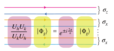
Figure 3: The boundary of the bulk with K matrix $K_{f}=\sigma_{z}\oplus K_{b}$ where $K_{b}$ is the K matrix for Type-III bosonic SPT phases in bosonic systems. The bosonic symmetry $G_{b}=(\mathbb{Z}_{n})^{3}$ with $n\geq 2$ only acts on the $K_{b}$ nontrivially. $|\Phi_{g}\rangle$, necessary being a multiplet, represent flux of one $\mathbb{Z}_{n}$ symmetry generated by $g$. $U_{h},U_{k}$ are the matrix representations of the elements $h,k$, the generators of the remaining $(\mathbb{Z}_{n})^{2}$ symmetry and they form the fundamental projective representation of $(\mathbb{Z}_{n})^{2}$. In our consruction, we conjecture $K_{b}=(\sigma_{x}){\oplus n-1}$ for $n\geq 2$. The shaded regions indicate that the symmetry realization of $h,k$ may permute different edge fields, as see (142), (144) and (152) and the creation operator for $g$ symmetry flux involves multiple edge fields.

V Type-III bosonic SPT embedded phases

Type-III bosonic SPT phases protected by $G_{b}$ would not be trivialized when embedding in fermionic system no matter how the $G_{b}$ extension by $\mathbb{Z}_{2}^{f}$. Using this fact, we can realize this kind of fSPT phase by considering the K matrix to be in the form of $K=\sigma_{z}\oplus\sigma_{x}\oplus...\oplus\sigma_{x}$. We also require that the realization of $G_{f}$ symmetry on the first fermionic block is trivial, namely we can symmetrically gap out the edge fields corresponding to the first block. Therefore, the symmetry anomaly of the edge fields would come from the bosonic block, namely the $K_{b}=\sigma_{x}\oplus...\oplus\sigma_{x}$ (see Fig.3). For this consideration, in the following, we will only consider the realization of symmetry on $K_{b}$ which may give rise to the type-III anomaly.

We here come up with a construction which can realize the Type-III bosonic SPT phases, instead of exausting all possible solutions. For $G_{b}=\mathbb{Z}_{n}\times\mathbb{Z}_{n}\times\mathbb{Z}_{n}$, we denote the generators of this group as $g_{1},g_{2},g_{3}$. We take $K_{b}$ to be the one consisting of $n-1$ block of $\sigma_{x}$, namely $K_{b}=\sigma_{x}\oplus...\oplus\sigma_{x}$ where there are $(n-1)$ $\sigma_{x}$ in the direct sum. The construction takes

$$W^{g_{1}}=1_{2(n-1)\times 2(n-1)},W^{g_{2}}=A,W^{g_{3}}=A^{n-1}.$$

The definition of $A$ is

$$A=\tilde{U}UM(\tilde{U}U)^{-1}$$

where $M=1_{2\times 2}\otimes\tilde{M}$ with

$$\tilde{M}=\begin{pmatrix}0_{\tilde{n}\times 1}&1_{\tilde{n}\times\tilde{n}}\\ -1&-1_{1\times\tilde{n}}\end{pmatrix}$$ (139)

for $\tilde{n}\equiv n-2\geq 1$ and $\tilde{M}=-1$ for $\tilde{n}=0$, and

$$U=\begin{pmatrix}1_{\bar{n}\times\bar{n}}&1_{\bar{n}\times\bar{n}}\\ 1_{\bar{n}\times\bar{n}}-O_{\bar{n}\times\bar{n}}&O_{\bar{n}\times\bar{n}}-1_{\bar{n}\times\bar{n}}\end{pmatrix}$$ (140)

with $\bar{n}\equiv n-1$ and $\tilde{U}$ is the integer unimodular matrix that transforms $K_{b}^{\prime}=\sigma_{x}\otimes 1_{(n-1)\times(n-1)}$ in $K_{b}=(\tilde{U}^{-1})^{T}K_{b}^{\prime}\tilde{U}^{-1}$. It can be checked that $M$ is an order-$n$ matrix, therefore $A^{n}=1_{2(n-1)\times 2(n-1)}$. $O_{\bar{n}\times\bar{n}}$ is an off-diagonal matrix whose elements $O_{i,j}=\delta_{i+1,j}$. The second part of the construction is the values of $\delta\phi^{g_{1,2,3}}$, which depend on $n$. To obtain the proper values of $\delta\phi^{g_{i}}=\frac{2\pi}{n}t_{i}$, we need to take into account the following sufficient conditions

(1) $t_{i}+W^{g_{i}}\cdot t_{j}=t_{j}+W^{g_{j}}\cdot t_{i}$ mod $n$, for all $i>j$

(2)$|(K_{b}^{-1}\cdot t_{1})^{T}\cdot(A^{k}-1_{2\bar{n}\times 2\bar{n}})\cdot t_{3}|=k$ mod $n^{2}$ for all $k=0,1,...,n-1$.

The first condition ensures that the generator $g_{i}$ and $g_{j}$ commute when acting on the basis of local Hilbert space, which is generated by $e^{i\phi_{i}},i=1,...,2n-2$. The second condition ensures that when acting on the symmetry flux corresponding to $g_{1}$, the $\mathbb{Z}_{n}\times\mathbb{Z}_{n}$ subgroup generated by $g_{2,3}$ form the fundamental projective representation. More precisely,

$$U_{g_{2}}=\begin{pmatrix}0&1_{n-1\times n-1}\\ 1&0\end{pmatrix},U_{g_{3}}=\alpha\begin{pmatrix}0&0&...&0&1\\ w&0&...&0&0\\ 0&w^{2}&0&\cdots&0\\ ...&...&...&...&...\\ 0&0&...&w^{n-1}&0\end{pmatrix}$$ (141)

where $\alpha$ is a constant phase factor and $w=e^{\pm i\frac{2\pi}{n}}$ (see Fig.3). We believe that the solution of $t_{i}$ always exists for general $n$, even though we can not prove here.

V.1 $G_{b}=\mathbb{Z}_{n}\times\mathbb{Z}_{n}\times\mathbb{Z}_{n}$: $n$ is odd

For $n=3$, $K_{b}=\sigma_{x}\oplus\sigma_{x}$, $W^{g_{1}}=1_{4\times 4}$, $W^{g_{2}}=A_{3}$, $W^{g_{3}}=(A_{3})^{2}$ with

$$A_{3}=\begin{pmatrix}0&0&-1&0\\ 0&-1&0&-1\\ 1&0&-1&0\\ 0&1&0&0\end{pmatrix},$$ (142)

and $\phi^{g_{1}}=\frac{2\pi}{3}(1,0,-1,0)^{T}$ mod $2\pi$, $\delta\phi^{g_{2}}=0$, $\delta\phi^{g_{3}}=\frac{2\pi}{3}(0,1,0,1)^{T}$ mod $2\pi$. Thereby $t_{1}=(1,0,-1,0)^{T}$, $t_{2}=0$, and $t_{3}=(0,1,0,1)^{T}$. As discused above, to check that the symmetry $g_{i},g_{j}$ acting on the local excitation $e^{i\phi_{i}}$ with $i=1,2,...,2n-2$ commute, we calculate

$$(1_{4\times 4}-W^{g_{2}})t_{1}-(1_{4\times 4}-W^{g_{1}})t_{2}=(0,0,-3,0)^{T}$$

$$(1_{4\times 4}-W^{g_{3}})t_{1}-(1_{4\times 4}-W^{g_{1}})t_{3}=(3,0,0,0)^{T}$$

$$(1_{4\times 4}-W^{g_{2}})t_{3}-(1_{4\times 4}-W^{g_{3}})t_{2}=(0,3,0,0)^{T}$$

which indicates that $g_{i},g_{j}$ indeed commute.

We now calculate the matrix representation of $\mathbb{Z}_{3}\times\mathbb{Z}_{3}$ generated by $g_{2,3}$ on the symmetry flux of the subgroup $\mathbb{Z}_{3}$ generated $g_{1}$, which is represented by the fractional vector $l_{g}=\frac{1}{3}(0,1,0,-1)^{T}$. Under symmetry $g_{2}$ or $g_{3}$, the $g_{1}$ flux represented by $l_{g_{1}}$ transform to $A_{3}^{T}l_{g_{1}}$ or $(A_{3}^{T})^{2}l_{g_{1}}$ which are equivalent to $l_{g_{1}}$; under $(g_{2})^{2}$ or $(g_{3})^{2}$, $l_{g_{1}}$ transform to $(A_{3}^{T})^{2}l_{g_{1}}$ or $A_{3}^{T}l_{g_{1}}$. Therefore, the $g_{1}$ symmetry flux forms a triplet $\{e^{il_{g_{1}}^{T}\cdot\phi},e^{il_{g_{1}}^{T}\cdot A_{3}\cdot\phi},e^{il_{g_{1}}^{T}\cdot(A_{3})^{2}\cdot\phi}\}$ that $g_{2},g_{3}$ act on. We compute the phase factors of the triplet under symmetry by

$$l_{g_{1}}^{T}(A_{3}-1)t_{3}=1$$

$$l_{g_{1}}^{T}[(A_{3})^{2}-1]t_{3}=-1.$$

Correspondingly, the matrix representation of $g_{2,3}$ on the triplet take

$$U_{g_{2}}=\begin{pmatrix}0&1&0\\ 0&0&1\\ 1&0&0\end{pmatrix},U_{g_{3}}=\begin{pmatrix}0&0&1\\ w&0&0\\ 0&w^{2}&0\end{pmatrix}$$ (143)

where $w=e^{-i\frac{2\pi}{3}}$. It is easy to check that $U_{g_{2}}U_{g_{3}}=wU_{g_{3}}U_{g_{2}}$ which suffices to show that they indeed form the fundamental projective representation of $\mathbb{Z}_{3}\times\mathbb{Z}_{3}$. It can also be checked that breaking this whole symmetry to any of it subgroup, the corresponding symmetry realization inherited can not protected any nontrivial phase. Therefore, we can conclude that this solution realize the pure Type-III root state.

For $n=5$, $K_{b}=(\sigma_{x})^{\oplus 4}$, $W^{g_{1}}=1_{8\times 8}$, $W^{g_{2}}=A_{5}$ and $W^{g_{3}}=(A_{5})^{4}$, with

$$A_{5}=\begin{pmatrix}0&0&0&1&-1&0&0&0\\ 0&0&1&0&0&0&0&0\\ 0&0&0&0&0&0&1&0\\ 0&0&0&0&-1&0&0&1\\ 1&0&0&0&-1&0&0&0\\ 0&1&0&0&0&0&0&0\\ 0&-1&-1&0&0&-1&-1&0\\ 0&0&0&0&-1&0&0&0\\ \end{pmatrix}$$ (144)

and $\delta\phi^{g_{2}}=\frac{2\pi}{5}(3,0,0,2,-1,0,0,1)^{T}$, $\delta\phi^{g_{2}}=0$, and $\delta\phi^{g_{3}}=\frac{2\pi}{5}(0,1,1,0,0,1,1,0)$. Accordingly, we have $t_{1}=(3,0,0,2,-1,0,0,1)^{T}$, $t_{3}=(0,1,1,0,0,1,1,0)^{T}$ and $t_{2}=0$. As discused above, to check that the symmetry $g_{i},g_{j}$ acting on the local excitation $e^{i\phi_{i}}$ with $i=1,2,...,8$ commute, we calculate

$$(1_{4\times 4}-W^{g_{2}})t_{1}-(1_{4\times 4}-W^{g_{1}})t_{2}=(0,0,0,0,-5,0,0,0)^{T}$$

$$(1_{4\times 4}-W^{g_{3}})t_{1}-(1_{4\times 4}-W^{g_{1}})t_{3}=(5,0,0,0,0,0,0,0)^{T}$$

$$(1_{4\times 4}-W^{g_{2}})t_{3}-(1_{4\times 4}-W^{g_{3}})t_{2}=(0,0,0,0,0,5,0,0)^{T}$$

which indicates that $g_{i},g_{j}$ indeed commute. We compute the phase factors of the quintet under symmetry by

$$l_{g_{1}}^{T}(A_{5}-1)t_{3}=-1$$

$$l_{g_{1}}^{T}[(A_{5})^{2}-1]t_{3}=-2$$

$$l_{g_{1}}^{T}[(A_{5})^{3}-1]t_{3}=-3$$

$$l_{g_{1}}^{T}[(A_{5})^{4}-1]t_{3}=1.$$

Therefore, on the basis $\{e^{il_{g_{1}}^{T}\cdot(A_{5})^{i}\cdot\phi},i=0,1,...,4\}$ generated by the $g_{1}$ symmetry fluxes, $g_{2,3}$ act as

$$U_{g_{2}}=\begin{pmatrix}0&1&0&0&0\\ 0&0&1&0&0\\ 0&0&0&1&0\\ 0&0&0&0&1\\ 1&0&0&0&0\end{pmatrix},U_{g_{3}}=e^{i\frac{2\pi}{5}}\begin{pmatrix}0&0&0&0&1\\ w&0&0&0&0\\ 0&w^{2}&0&0&0\\ 0&0&w^{3}&0&0\\ 0&0&0&w^{4}&0\end{pmatrix}$$ (145)

where $w=e^{-i\frac{2\pi}{5}}$. It is easy to check that $U_{g_{2}}U_{g_{3}}=wU_{g_{3}}U_{g_{2}}$ which suffices to show that $U_{g_{2,3}}$ form the fundamental projective representation of $\mathbb{Z}_{5}\times\mathbb{Z}_{5}$. We do not show that the constrution realizes the pure Type-III bosonic SPT phase, and it may contain the other component(s) of bosonic SPT phase(s) protected by subgroups of $\mathbb{Z}_{5}\times\mathbb{Z}_{5}\times\mathbb{Z}_{5}$. However, it does not matter since we can stacking the inverse of extra phase to cancel it, leaving the pure Type-III root phase.

V.2 $G_{b}=\mathbb{Z}_{n}\times\mathbb{Z}_{n}\times\mathbb{Z}_{n}$: $n$ is even

For $n=2$, $K_{b}=\sigma_{x}$, $W^{g_{1}}=1_{2\times 2}$, $W^{g_{2,3}}=-1_{2\times 2}$, and $\delta\phi^{g_{1}}=\pi(1,0)^{T}$, $\delta\phi^{g_{2}}=0$, $\delta\phi^{g_{3}}=\pi(0,1)^{T}$. In fact, for this realization of symmetry any subgroup of $\mathbb{Z}_{2}\times\mathbb{Z}_{2}\times\mathbb{Z}_{2}$ can not protect a nontrivial phase, but the whole the symmetry can. This fact already indicates that this solution realizes the Type-III bosonic SPT phase protected by $\mathbb{Z}_{2}\times\mathbb{Z}_{2}\times\mathbb{Z}_{2}$. To further comfirm this fact, we can alse check that subgroup $\mathbb{Z}_{2}\times\mathbb{Z}_{2}$ generated by $g_{2,3}$ forms the projective representation when acting on the symmetry flux of $g_{1}$. The symmetry flux of $g_{1}$ is related to the ”fractionalied” vetex operator $e^{i\frac{1}{2}\phi_{1}}$. Then on the basis of $(e^{i\frac{1}{2}\phi_{2}},e^{-i\frac{1}{2}\phi_{2}})$, $g_{2}$ acts as $\sigma_{x}$ while $g_{2}$ acts as $-\sigma_{y}$, therefore, they form the projective representation of $\mathbb{Z}_{2}\times\mathbb{Z}_{2}$ group. We make a remark about the construction of this case, that is the same construction can also be obtained from a free fermion construction.

For $n=4$, $K_{b}=\sigma_{x}\oplus\sigma_{x}\oplus\sigma_{x}$, and $W^{g_{1}}=1$, $W^{g_{2}}=A_{4},W^{g_{3}}=(A_{4})^{3}$ with

$$A_{4}=\left(\begin{array}[]{cccccc}0&0&-1&0&0&0\\ 0&-1&0&-1&-1&0\\ 0&0&-1&0&0&1\\ 0&0&0&0&1&0\\ 0&1&0&0&0&0\\ 1&0&-1&0&0&0\\ \end{array}\right),$$ (152)

and $\delta\phi^{g_{1}}=\pi/2(1,0,-1,0,0,2)^{T}$ mod $2\pi$, $\delta\phi^{g_{2}}=0$ and $\delta\phi^{g_{3}}=\pi/2(0,1,0,1,1,0)^{T}$ mod $2\pi$. Accordingly, we have $t_{1}=(1,0,-1,0,0,2)^{T}$, $t_{3}=(0,1,0,1,1,0)^{T}$ and $t_{2}=0$. As discused above, to check that the symmetry $g_{i},g_{j}$ acting on the local excitation $e^{i\phi_{i}}$ with $i=1,2,...,6$ commute, we calculate

$$(1_{4\times 4}-W^{g_{2}})t_{1}-(1_{4\times 4}-W^{g_{1}})t_{2}=(0,0,-4,0,0,0)^{T}$$

$$(1_{4\times 4}-W^{g_{3}})t_{1}-(1_{4\times 4}-W^{g_{1}})t_{3}=(0,0,0,0,0,4)^{T}$$

$$(1_{4\times 4}-W^{g_{2}})t_{3}-(1_{4\times 4}-W^{g_{3}})t_{2}=(0,0,0,4,0,0)^{T}$$

which indicates that $g_{i},g_{j}$ indeed commute. The phase factors of the quartet under symmetry is given by

$$l_{g_{1}}^{T}(A_{4}-1)t_{3}=-1$$

$$l_{g_{1}}^{T}[(A_{4})^{2}-1]t_{3}=-2$$

$$l_{g_{1}}^{T}[(A_{4})^{3}-1]t_{3}=1.$$

To see that the solution realizes the phase that contain the type-III root state, we check that the matrix representation of $\mathbb{Z}_{4}\times\mathbb{Z}_{4}$ generated by $g_{2,3}$ forms the fundamental projective representation when acting on the symmetry flux of the subgroup $\mathbb{Z}_{4}$ generated $g_{1}$, which is represented by the fractional vector $l_{g}=\frac{1}{4}(0,1,0,-1,2,0)^{T}$. More explicitly, $g_{2,3}$ take

$$U_{g_{2}}=\begin{pmatrix}0&1&0&0\\ 0&0&1&0\\ 0&0&0&1\\ 1&0&0&0\end{pmatrix},U_{g_{3}}=e^{i\frac{\pi}{4}}\begin{pmatrix}0&0&0&1\\ w&0&0&0\\ 0&w^{2}&0&0\\ 0&0&w^{3}&0\end{pmatrix}$$ (153)

where $w=e^{-i\frac{\pi}{2}}$. It is easy to check that $U_{g_{2}}U_{g_{3}}=wU_{g_{3}}U_{g_{2}}$ which suffice to show that they indeed form the fundamental projective representation of $\mathbb{Z}_{4}\times\mathbb{Z}_{4}$.

Though we do not show that the constrution realizes the pure Type-III bosonic SPT phase, it does not matter since we can stacking the inverse of extra phase to cancel other component which is more easy to obtain, leaving the pure Type-III root phase.

For more other $n$, using the above construction, the solution of Type-III bosonic SPT phase can be constructed. Though lacking rigorous proof, we believe that the above construction can be used to find any value of $n$.

VI Intrinsically interacting fSPT

In this section, we first construct a solution that can realize root state of intrinsically interacting phases of $\mathbb{Z}_{4}^{f}\times\mathbb{Z}_{4}\times\mathbb{Z}_{4}$ fSPT. The fingerprint of the root state is that $\frac{\pi}{2}$ flux of $\mathbb{Z}_{4}^{f}$ carries fundamental projective representation of the remaining $\mathbb{Z}_{4}\times\mathbb{Z}_{4}$ (see Fig.4). We also show that it is the square root of the fundamental phase of Type-III bosonic SPT protected by symmetry $\mathbb{Z}_{2}\times\mathbb{Z}_{4}\times\mathbb{Z}_{4}$.

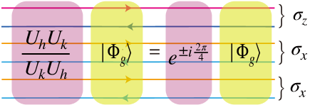
Figure 4: The K matrix for intrinsically interacting fSPT protected by $\mathbb{Z}_{4}^{f}\times\mathbb{Z}_{4}\times\mathbb{Z}_{4}$ symmetry is $K=\sigma_{z}\oplus\sigma_{x}\oplus\sigma_{x}$. $|\Phi_{g}\rangle$ represents $\frac{\pi}{2}$ flux of $\mathbb{Z}_{4}^{f}$ whose generator is denoted as $g$ and $U_{h},U_{k}$ are the matrix representation of the generators $h,k$ of the remaining $\mathbb{Z}_{4}\times\mathbb{Z}_{4}$. The shaded regions indicate that the symmetry realization of $h,k$ may permute different edge fields, including the fermionic ones, as see (161) and the $\frac{\pi}{2}$ symmetry flux is a multiplet that invovles different edge fields.

The K matrix takes

$$K_{f}=\sigma_{z}\oplus\sigma_{x}\oplus\sigma_{x}$$ (154)

The symmetry generators for $\mathbb{Z}_{4}^{f}\times\mathbb{Z}_{4}\times\mathbb{Z}_{4}$ is $g,h,k$ with $g^{2}=P_{f}$ and $h^{4}=k^{4}=1$. The symmetry realization on the edge fields for the intrinsic interacting fSPT phase takes $W^{g}=1_{6\times 6}$, $W^{h}=\tilde{A}_{4},W^{k}=\tilde{A}_{4}^{-1}=(\tilde{A}_{4})^{3}$ where

$$\tilde{A}_{4}=\left(\begin{array}[]{cccccc}1&0&0&-2&0&-1\\ 0&1&0&2&0&-1\\ 0&0&0&0&0&1\\ 1&-1&0&-2&1&0\\ 0&0&0&1&0&0\\ 2&2&1&0&0&-2\\ \end{array}\right),$$ (161)

and $\delta\phi^{g}=\frac{\pi}{2}(1,1,0,0,0,0)^{T}$, $\delta\phi^{h}=0$ and $\delta\phi^{k}=\frac{\pi}{2}(2,0,2,1,1,2)^{T}$. To see it indeed corresponds to the edge theory of intrinsically interacting fSPT phase, now we check the following points. First of all, the symmetry realization of $g$ is consistent with the fact that $g^{2}=P_{f}$ where $P_{f}$ is conventionally realized as $W^{P_{f}}=1$ and $\delta\phi^{P_{f}}=\pi(1,1,0,0,0,0)^{T}$. Namely the fermion get $\pi$ phase under $P_{f}$ while boson is invariant up to $2\pi$ phase shift. Secondly, this symmetry realization of $g_{1},g_{2},g_{3}$ on the local excitaitons $e^{i\phi_{i}}$, with $i=1,2,...,6$ commute with each other, which can be easily confirmed by calculating

$$(1_{4\times 4}-W^{h})\delta\phi^{g}-(1_{4\times 4}-W^{g})\delta\phi^{h}=(0,0,0,0,0,-2\pi)^{T}$$

$$(1_{4\times 4}-W^{k})\delta\phi^{g}-(1_{4\times 4}-W^{g})\delta\phi^{k}=(0,0,2\pi,0,0,0)^{T}$$

$$(1_{4\times 4}-W^{h})\delta\phi^{k}-(1_{4\times 4}-W^{k})\delta\phi^{h}=(2\pi,0,0,0,0,0)^{T}.$$

Finally, we check that the $g$-flux (i.e., $\frac{\pi}{2}$ flux defects of $\mathbb{Z}_{4}^{f}$) carries the projective representation of $\mathbb{Z}_{4}\times\mathbb{Z}_{4}$ generated by $h,k$. The $g$-flux excitation corresponds to the fractional vector $l_{g}=\frac{K_{f}}{2\pi}\delta\phi^{g}=\frac{1}{4}(1,-1,0,0,0,0)^{T}$. The $g$-flux excitations form a quartet $\{e^{il_{g}^{T}\cdot\phi},e^{il_{g}^{T}\cdot\tilde{A}_{4}\cdot\phi},e^{il_{g}^{T}\cdot(\tilde{A}_{4})^{2}\cdot\phi},e^{il_{g}^{T}\cdot(\tilde{A}_{4})^{3}\cdot\phi}\}$ under the symmetry of $h,k$. We compute the phase factors of the quartet under symmetry action $k$ as

$$l_{g}^{T}(\tilde{A}_{4}-1)\delta\phi^{k}=-\pi/2$$

$$l_{g}^{T}[(\tilde{A}_{4})^{2}-1]\delta\phi^{k}=-\pi$$

$$l_{g}^{T}[(\tilde{A}_{4})^{3}-1]\delta\phi^{k}=\pi/2.$$

From the realization and relation above, we have the represenation on the quartet of $\mathbb{Z}_{4}\times\mathbb{Z}_{4}$ generated by $h,k$ as

$$U^{h}=\begin{pmatrix}0&1&0&0\\ 0&0&1&0\\ 0&0&0&1\\ 1&0&0&0\end{pmatrix},\,U^{k}=e^{i\frac{\pi}{4}}\begin{pmatrix}0&0&0&1\\ w&0&0&0\\ 0&w^{2}&0&0\\ 0&0&w^{3}&0\end{pmatrix}$$ (162)

with $w=e^{-i\frac{\pi}{2}}$. Therefore, $U^{h,k}$ form the fundemental projective rerpresentation of $\mathbb{Z}_{4}\times\mathbb{Z}_{4}$.

Now we argue that coupled system stacking two these root phases is equivalent to the bosonic Type-III SPT embedded phase protected by $\mathbb{Z}_{2}\times\mathbb{Z}_{4}\times\mathbb{Z}_{4}$. To show the argument, we check check the projective representation of $\mathbb{Z}_{4}\times\mathbb{Z}_{4}$ carried by $g$-defect. K matrix of the stacking system now is

$$K_{s}=K_{f}\oplus K_{f}$$ (163)

where $K_{f}$ is the one in (154). The symmetry realization on the edge theory of this system takes $W_{s}^{g}=W^{g}\oplus W^{g}$, $W_{s}^{h}=W^{h}\oplus W^{h}$ and $W_{s}^{k}=W^{k}\oplus W^{k}$ and $\delta\phi_{s}^{g}=\delta\phi^{g}\oplus\delta\phi^{g}$, $\delta\phi_{s}^{h}=\delta\phi^{h}\oplus\delta\phi^{h}$ and $\delta\phi_{s}^{k}=\delta\phi^{k}\oplus\delta\phi^{k}$. Similrly, the $g$-defect corresponds to the fractional vector $\tilde{l}_{g}=\frac{K_{s}}{2\pi}\delta\phi_{s}^{g}=\frac{1}{4}(1,-1,0,0,0,0,1,-1,0,0,0,0)^{T}$ and also form a quartet $\{e^{i\tilde{l}_{g}^{T}\cdot\phi},e^{i\tilde{l}_{g}^{T}\cdot A_{s}\cdot\phi},e^{i\tilde{l}_{g}^{T}\cdot A_{s}^{2}\cdot\phi},e^{i\tilde{l}_{g}^{T}\cdot A_{s}^{3}\cdot\phi}\}$ where $A_{s}=A\oplus A$. Therefore, the projective representation of $\mathbb{Z}_{4}\times\mathbb{Z}_{4}$ carried by $g$-defect takes

$$U_{s}^{h}=\begin{pmatrix}0&1&0&0\\ 0&0&1&0\\ 0&0&0&1\\ 1&0&0&0\end{pmatrix},\,U_{s}^{k}=e^{\tilde{i}l_{g}^{T}\cdot\delta\phi_{s}^{k}}\begin{pmatrix}0&0&0&1\\ -1&0&0&0\\ 0&1&0&0\\ 0&0&-1&0\end{pmatrix}$$ (164)

It is easy to check that

$$\tilde{U}_{h}\tilde{U}_{k}=-\tilde{U}_{k}\tilde{U}_{h}$$ (165)

which indicates that $\tilde{U}_{h}$ and $\tilde{U}_{k}$ form the projective representation of $\mathbb{Z}_{4}\times\mathbb{Z}_{4}$ and this projective representation is the square of the root one, as in (162). It can also be calculated similarly that the representation of $\mathbb{Z}_{4}\times\mathbb{Z}_{4}$ carried by $\pi$-flux(i.e. $P_{f}$ flux) is linear. Therefore, the representation carried by $g$-defect is the same as that in the bosonic Type-III SPT embedded phases, indicating the phase realized in this stacking system is consistent with the bosonic Type-III SPT embedded phases.

VII Conclusion and Discussion

In this paper, we obtain the edge theories of 2D fSPT protected by unitary Abelian total symmetry group $G_{f}$ by utilizing the K matrix formulation of Abelian Chern-Simions theory. These edge theories admit the anomalous symmetry actions that prevent the edge being a symmetric gapped state. In fact, for a specific $K$ matrix and total symmetry $G_{f}$, we can obtain many different realizations of symmetry action for the edge fields. Some of them are anomaly-free, while some are anomalous. Among various anomalous edge theories, we identify the root state(s) and also show how others are related to the root one(s). Although without having a general formulation, we consider some representative unitary Abelian total symmetries $G_{f}$ including both trivial or nontrivial central extension over $\mathbb{Z}_{2}^{f}$. These discussion can be generalized into arbitrary unitary Abelian total symmetry $G_{f}$.

Moreover, we also construct the Luttinger liquid edge theories of Type-III bosonic SPT protected by $(\mathbb{Z}_{n})^{3}$ for the first time. We note that an edge theory can be described by three data $[K,\{W^{g_{i}},\delta\phi^{g^{i}}\}]$. In our construction, the $K$ matrix is chosen as $K=(\sigma_{x})^{\oplus(n-1)}$, which indicates the central charge of edge theory is $n-1$. The key construction is the general expression of $W^{g_{i}}$ for general $n$, which can be used to obtain the proper $\{\delta\phi^{g_{i}}\}$ that give rise to the correct anomalous symmetry action for any Type-III bosonic SPT root states. We explicitly show that the solution for $\delta\phi^{g_{i}}$ with $n=2,3,4,5$ and we believe that our construction indeed can be applied to arbitrary $n$. Technically, one shall pay attention to the constraints from the linear representation of group on the basis of local excitations and derive the projective representation of two $\mathbb{Z}_{n}$s on symmetry flux of the third subgroup. We stress that even though 1+1D $SU(n)_{1}$ WZW model can be constructed from the $n-1$ components Luttinger liquid with a fine-tuning radius, our construction does not have constraint on the radius, which implies that the edge theory can flow away from the previously conjectured $SU(n)_{1}$ point by some relevant symmetric interaction. It is interesting to study the stability of the $SU(n)_{1}$ WZW model with such symmetry realization on the lattice model. Related to this question, Ref.[64] study the similar question in a 1+1D spin chain with a similar anomaly, the so-called LSM anomaly.

More interestingly, we also discuss the edge theory of the so-called intrinsically interacting fSPT. The minimal symmetry protecting this kind of phases is $\mathbb{Z}_{4}^{f}\times\mathbb{Z}_{4}\times\mathbb{Z}_{2}^{T}$, whose edge theories are studied in Ref.[65]. For the unitary Abelian $G_{b}$, the minimal one is $\mathbb{Z}_{4}^{f}\times\mathbb{Z}_{4}\times Z_{4}$. We construct the corresponding edge theory for the root state of $\mathbb{Z}_{4}^{f}\times\mathbb{Z}_{4}\times Z_{4}$ intrinsically interacting fSPT. It is very interesting to compare this case with the Type-III bosonic SPT state. Upon gauging one $\mathbb{Z}_{4}$ in the former or $\mathbb{Z}_{4}^{f}$ in the latter, we both obtain $\mathbb{Z}_{4}$ toric code enriched by $\mathbb{Z}_{4}\times\mathbb{Z}_{4}$ symmetry, but with different symmetry fractionalization on anyons. For the $\mathbb{Z}_{4}$ gauged Type-III bosonic SPT state, the $\mathbb{Z}_{4}$ gauge charge is bosonic, and $\mathbb{Z}_{4}$ flux carries the fundamental projective representation of remaining $\mathbb{Z}_{4}\times\mathbb{Z}_{4}$ symmetry. In contrast, for the $\mathbb{Z}_{4}^{f}$ gauged fSPT, the $\mathbb{Z}_{4}^{f}$ gauge charge is fermionic and $\mathbb{Z}_{4}^{f}$ flux carries the fundamental projective representation of remaining $\mathbb{Z}_{4}\times\mathbb{Z}_{4}$ symmetry. Based these observations, starting from the $\mathbb{Z}_{4}$ toric code enriched by $\mathbb{Z}_{4}\times\mathbb{Z}_{4}$ symmetry, to obtain the Type-III bosonic SPT, one may condense some bosons(such as the nuetral bosonic gauge charge), while for intrinsically interacting fSPT, one should condense the fermion that does not carries projective representation of $\mathbb{Z}_{4}\times\mathbb{Z}_{4}$. Such understanding can be generalized to other intrinsically interacting fSPT. In fact, the basic concept of boson/fermion condensation is also very useful to understand the gapless edge theory of symmetry enriched topological(SET) phases, and we will study more examples in our future works.

SQN especially acknowledges Meng Cheng for sharing his theory on anomaly of 1+1D CFT and insightful discussion on the construction on edge theories of Type-III bosonic SPT. SQN and CW are supported by the Research Grant Council of Hong Kong (ECS 21301018, GRF 11300819) and URC, HKU (Grant No. 201906159002). QRW and ZCG are supported by the Research Grant Council of Hong Kong (GRF No.14306918, ANR/RGC Joint Research Scheme No. A-CUHK402/18) , and Direct Grant No. 4053346 from The Chinese University of Hong Kong.

Appendix A Other solutions of $\mathbb{Z}_{2}\times\mathbb{Z}_{2}\times\mathbb{Z}_{2}^{f}$ symmetry

1. Solutions with $W^{g_{1}}=W^{g_{2}}=1_{2\times 2}$

From (83b) and (83c), we have

$$\delta\phi^{g_{1}}=\pi\begin{pmatrix}t_{1}^{g_{1}}\\ t_{2}^{g_{1}}\end{pmatrix},\quad\delta\phi^{g_{2}}=\pi\begin{pmatrix}t_{1}^{g_{2}}\\ t_{2}^{g_{2}}\end{pmatrix},\quad t_{1,2}^{g_{1,2}}=0,1$$ (166)

The (83d) does not give any new constraint. We then denote these solutions as $[1_{2\times 2},1_{2\times 2},(t_{1}^{g_{1}},t_{2}^{g_{1}}),(t_{1}^{g_{2}},t_{2}^{g_{2}})]$. Similar to the case discussed in Sec.III.2.4, we have

$$[1_{2\times 2},1_{2\times 2},(t_{1}^{g_{1}},t_{2}^{g_{1}}),(t_{1}^{g_{2}},t_{2}^{g_{2}})]$$

$$\oplus [1_{2\times 2},1_{2\times 2},(t_{2}^{g_{1}},t_{1}^{g_{1}}),(t_{2}^{g_{2}},t_{1}^{g_{2}})]=1$$ (167)

and

$$[1_{2\times 2},1_{2\times 2},(t_{1}^{g_{1}},t_{1}^{g_{1}}),(t_{1}^{g_{2}},t_{1}^{g_{2}})]=1$$ (168)

Therefore, we only need to consider the following six cases: $[1_{2\times 2},1_{2\times 2},(0,0),(0,1)]$, $[1_{2\times 2},1_{2\times 2},(0,1),(0,0)]$, $[1_{2\times 2},1_{2\times 2},(0,1),(0,1)]$, $[1_{2\times 2},1_{2\times 2},(0,1),(1,0)]$, $[1_{2\times 2},1_{2\times 2},(0,1),(1,1)]$ and $[1_{2\times 2},1_{2\times 2},(1,1),(0,1)]$.

1.1 Solution: $[1_{2\times 2},1_{2\times 2},(0,0),(0,1)]$

We can show that

$$[1_{2\times 2},1_{2\times 2},(0,0),(0,1)]=[1_{2\times 2},\sigma_{z},(0,0),0]^{\oplus 2}$$ (169)

whose structure factor is

$$r([1_{2\times 2},1_{2\times 2},(0,0),(0,1)])=(0,2,0).$$ (170)

To show (169), we consider the stacking system

$$[1_{2\times 2},\sigma_{z},(0,0),0]^{\oplus 2}\oplus[1_{2\times 2},1_{2\times 2},(0,0),(1,0)].$$ (171)

We denote the edge bosonic fields of these three states by $\phi_{1}^{(1)},\phi_{2}^{(1)},\phi_{1}^{(2)},\phi_{2}^{(2)},\phi_{1},\phi_{2}$. Under symmetry,

$$g_{1}:\begin{pmatrix}\phi_{1}^{(\alpha)}\\ \phi_{2}^{(\alpha)}\end{pmatrix}\rightarrow\begin{pmatrix}\phi_{1}^{(\alpha)}\\ \phi_{2}^{(\alpha)}\end{pmatrix}$$ (172)

$$g_{2}:\begin{pmatrix}\phi_{1}^{(\alpha)}\\ \phi_{2}^{(\alpha)}\end{pmatrix}\rightarrow\begin{pmatrix}\phi_{1}^{(\alpha)}\\ -\phi_{2}^{(\alpha)}\end{pmatrix}$$ (173)

$$g_{1}:\begin{pmatrix}\phi_{1}\\ \phi_{2}\end{pmatrix}\rightarrow\begin{pmatrix}\phi_{1}\\ \phi_{2}\end{pmatrix}$$ (174)

$$g_{2}:\begin{pmatrix}\phi_{1}\\ \phi_{2}\end{pmatrix}\rightarrow\begin{pmatrix}\phi_{1}+\pi\\ \phi_{2}\end{pmatrix}$$ (175)

where $i,\alpha=1,2$. We define the following majorana fermions through the bosonic edge fields by

$$\eta_{R}^{1}+i\eta_{R}^{2}=\frac{1}{\sqrt{\pi}}e^{i\phi_{2}},\,\eta_{L}^{1}+i\eta_{L}^{2}=\frac{1}{\sqrt{\pi}}e^{-i\phi_{1}},$$ (176)

$$\xi_{R}^{\alpha 1}+i\xi_{R}^{\alpha 2}=\frac{1}{\sqrt{\pi}}e^{i\phi_{2}^{(\alpha)}},\,\xi_{L}^{\alpha 1}+i\xi_{L}^{\alpha 2}=\frac{1}{\sqrt{\pi}}e^{-i\phi_{1}^{(\alpha)}},$$ (177)

which under symmetry transform as

$$g_{1}:\, \eta_{R}^{i}\rightarrow\eta_{R}^{i},\,\eta_{L}^{i}\rightarrow\eta_{L}^{i},$$ (178)

$$g_{2}:\, \eta_{R}^{i}\rightarrow\eta_{R}^{i},\,\eta_{L}^{i}\rightarrow-\eta_{L}^{i},$$ (179)

$$g_{1}:\, \xi_{R}^{\alpha i}\rightarrow\xi_{R}^{\alpha j},\,\xi_{L}^{\alpha i}\rightarrow\xi_{L}^{\alpha i}$$ (180)

$$g_{2}:\, \xi_{R}^{\alpha i}\rightarrow(-1)^{i-1}\xi_{R}^{\alpha i},\,\xi_{L}^{\alpha i}\rightarrow\xi_{L}^{\alpha i}$$ (181)

where $i,j,\alpha=1,2$ and the repeated $j$ is summed. These twelve majorana fermions can be gapped out by the following symmetric mass terms

$$im_{i}\eta_{R}^{i}\xi_{L}^{1i}+i\tilde{m}_{i}\xi_{R}^{i2}\eta_{L}^{i}+i\hat{m}_{i}\xi_{R}^{i1}\xi_{L}^{2i}$$ (182)

where repreated index $i$ is summed. Therefore, the stacking system (171) is trivial and then the relation (169) is proved.

1.2 Solution: $[1_{2\times 2},1_{2\times 2},(0,1),(0,0)]$

Similar to the $Solution\,1.1$, we have

$$[\sigma,1_{2\times 2},0]\oplus[\sigma,1_{2\times 2},0]=[1_{2\times 2},1_{2\times 2},(0,1),(0,0)]$$ (183)

which means by using the three-component vector,

$$r([1_{2\times 2},1_{2\times 2},(0,1),(0,0)])=(2,0,0).$$ (184)

1.3 Solution: $[1_{2\times 2},1_{2\times 2},(0,1),(0,1)]$

For this case, we will show that

$$[1_{2\times 2},1_{2\times 2},(0,1),(0,1)]\oplus[1_{2\times 2},1_{2\times 2},(1,0),(0,0)]$$

$$[1_{2\times 2},1_{2\times 2},(0,0),(1,0)]\oplus[-1_{2\times 2},-1_{2\times 2},0,1]^{\oplus 2}=1.$$ (185)

We denote the two bosonic edge fields of the five phases in the above stacking system as $\phi_{1,2}$, $\varphi_{1,2}$, $\tilde{\varphi}_{1,2}$, $\rho^{1}_{1,2}$ and $\rho^{2}_{1,2}$ respectively, which transform under symmetry as

$$g_{1}:\begin{pmatrix}\phi_{1}\\ \phi_{2}\\ \varphi_{1}\\ \varphi_{2}\\ \tilde{\varphi}_{1}\\ \tilde{\varphi}_{2}\\ \rho^{a}_{1}\\ \rho^{a}_{2}\end{pmatrix}\rightarrow\begin{pmatrix}\phi_{1}\\ \phi_{2}+\pi\\ \varphi_{1}+\pi\\ \varphi_{2}\\ \tilde{\varphi}_{1}\\ \tilde{\varphi}_{2}\\ -\rho^{a}_{1}\\ -\rho^{a}_{2}+\pi\end{pmatrix},\,g_{2}:\begin{pmatrix}\phi_{1}\\ \phi_{2}\\ \varphi_{1}\\ \varphi_{2}\\ \tilde{\varphi}_{1}\\ \tilde{\varphi}_{2}\\ \rho^{a}_{1}\\ \rho^{a}_{2}\end{pmatrix}\rightarrow\begin{pmatrix}\phi_{1}\\ \phi_{2}+\pi\\ \varphi_{1}\\ \varphi_{2}\\ \tilde{\varphi}_{1}+\pi\\ \tilde{\varphi}_{2}\\ -\rho^{a}_{1}\\ -\rho^{a}_{2}\end{pmatrix}$$ (186)

Similar to (176), we define the following majorana fermions

$$\eta_{R,L}^{1}+i\eta_{R,L}^{2}=\frac{1}{\sqrt{\pi}}e^{\pm i\phi_{2,1}},$$ (187)

$$\xi_{R,L}^{1}+i\xi_{R,L}^{2}=\frac{1}{\sqrt{\pi}}e^{\pm i\varphi_{2,1}},$$ (188)

$$\chi_{R,L}^{1}+i\chi_{R,L}^{2}=\frac{1}{\sqrt{\pi}}e^{\pm i\tilde{\varphi}_{2,1}},$$ (189)

$$\gamma_{1R,1L}^{1}+i\gamma_{1R,1L}^{2}=\frac{1}{\sqrt{\pi}}e^{\pm i\rho^{1}_{2,1}},$$ (190)

$$\gamma_{2R,2L}^{1}+i\gamma_{2R,2L}^{2}=\frac{1}{\sqrt{\pi}}e^{\pm i\tilde{\rho}^{2}_{2,1}}.$$ (191)

We can fully gap out the edge fields of the stacking system by adding the following mass terms

$$im_{1i}\xi_{R}^{i}\eta_{L}^{i}+im_{2i}\eta_{R}^{i}\gamma_{iL}^{2}+im_{2i}\gamma_{iR}^{1}\xi_{L}^{i}$$

$$+im_{4i}\chi_{R}^{i}\gamma_{iL}^{1}+im_{5i}\gamma_{iR}^{2}\chi_{L}^{i}$$ (192)

where repeated $i$ is summed. The symmetry properties of these majorana fermions can be inherited from (198), and it turns out that all these mass terms are all symmetric. Therefore, the stacking system (185) is trivial. Further, from (167), (169) and (95), we can see the phase $[1_{2\times 2},1_{2\times 2},(0,1),(0,1)]$ is related to the three root states by

$$[1_{2\times 2},1_{2\times 2},(0,1),(0,1)]=[1_{2\times 2},\sigma_{z},(0,0),0]^{\oplus 2}\oplus$$

$$[\sigma_{z},1_{2\times 2},(0,0),0]^{\oplus 2}\oplus[-1_{2\times 2},-1_{2\times 2},0,1]^{\oplus 2}$$ (193)

which indicates that its structure factor is

$$r([1_{2\times 2},1_{2\times 2},(0,1),(0,1)])=(2,2,2).$$ (194)

1.4 Solution: $[1_{2\times 2},1_{2\times 2},(0,1),(1,0)]$

We can show that

$$[1_{2\times 2},1_{2\times 2},(0,1),(1,0)] =[1_{2\times 2},1_{2\times 2},(0,1),(0,0)]$$

$$\oplus[1_{2\times 2},1_{2\times 2},(0,0),(1,0)]$$ (195)

which indicates its structure factor is

$$r([1_{2\times 2},1_{2\times 2},(0,1),(1,0)])=(2,2,0).$$ (196)

To show (195), is equivalent to show that

$$[1_{2\times 2},1_{2\times 2},(0,1),(1,0)]\oplus[1_{2\times 2},1_{2\times 2},(1,0),(0,0)]$$

$$\oplus[1_{2\times 2},1_{2\times 2},(0,0),(0,1)]=1.$$ (197)

To show (195), we denote the bosonic edge fields of the three states by $\phi_{1,2}$, $\varphi_{1,2}$ and $\tilde{\varphi}_{1,2}$ respectively, which transform under symmetry as

$$g_{1}:\begin{pmatrix}\phi_{1}\\ \phi_{2}\\ \varphi_{1}\\ \varphi_{2}\\ \tilde{\varphi}_{1}\\ \tilde{\varphi}_{2}\end{pmatrix}\rightarrow\begin{pmatrix}\phi_{1}\\ \phi_{2}+\pi\\ \varphi_{1}+\pi\\ \varphi_{2}\\ \tilde{\varphi}_{1}\\ \tilde{\varphi}_{2}\end{pmatrix},\,g_{2}:\begin{pmatrix}\phi_{1}\\ \phi_{2}\\ \varphi_{1}\\ \varphi_{2}\\ \tilde{\varphi}_{1}\\ \tilde{\varphi}_{2}\end{pmatrix}\rightarrow\begin{pmatrix}\phi_{1}+\pi\\ \phi_{2}\\ \varphi_{1}\\ \varphi_{2}\\ \tilde{\varphi}_{1}\\ \tilde{\varphi}_{2}+\pi\end{pmatrix}$$ (198)

From these bosonic edge fields, we define the six majorana fermions as (187)-(189). We can fully gap out the edge fields by adding the mass terms

$$im_{1i}\eta_{R}^{i}\xi_{L}^{i}+im_{2i}\xi_{R}^{i}\chi_{L}^{i}+im_{3i}\chi_{R}^{i}\eta_{L}^{i}.$$ (199)

The symmetry properties can be inherited from those of bosonic edge fields, and it turns out that all the mass terms are symmetric. Therefore, the stacking system (197) is trivial.

1.5 Solution: $[1_{2\times 2},1_{2\times 2},(0,1),(1,1)]$

We can show that

$$[1_{2\times 2},1_{2\times 2},(0,1),(1,1)] =[1_{2\times 2},1_{2\times 2},(0,0),(1,0)]$$

$$\oplus[1_{2\times 2},1_{2\times 2},(0,1),(0,1)]$$ (200)

Since from (167) $[1_{2\times 2},1_{2\times 2},(0,0),(1,0)]$ is the inverse of $[1_{2\times 2},1_{2\times 2},(0,0),(0,1)]$, the structure factor of $[1_{2\times 2},1_{2\times 2},(0,1),(1,1)]$ is

$$r([1_{2\times 2},1_{2\times 2},(0,1),(1,1)])=(2,0,2).$$ (201)

which means that $[1_{2\times 2},1_{2\times 2},(0,1),(1,1)]$ is equivalent to $[1_{2\times 2},1_{2\times 2},(0,1),(0,0)]$. To show (205) is equivalent to show that

$$[1_{2\times 2},1_{2\times 2},(0,1),(1,1)]\oplus[1_{2\times 2},1_{2\times 2},(0,0),(1,0)]$$

$$\oplus[1_{2\times 2},1_{2\times 2},(1,0),(1,0)]=1.$$ (202)

To show (202), we denote the bosonic edge fields of the three states by $\phi_{1,2}$, $\varphi_{1,2}$ and $\tilde{\varphi}_{1,2}$ respectively, which transform under symmetry as

$$g_{1}:\begin{pmatrix}\phi_{1}\\ \phi_{2}\\ \varphi_{1}\\ \varphi_{2}\\ \tilde{\varphi}_{1}\\ \tilde{\varphi}_{2}\end{pmatrix}\rightarrow\begin{pmatrix}\phi_{1}\\ \phi_{2}+\pi\\ \varphi_{1}\\ \varphi_{2}\\ \tilde{\varphi}_{1}+\pi\\ \tilde{\varphi}_{2}\end{pmatrix},\,g_{2}:\begin{pmatrix}\phi_{1}\\ \phi_{2}\\ \varphi_{1}\\ \varphi_{2}\\ \tilde{\varphi}_{1}\\ \tilde{\varphi}_{2}\end{pmatrix}\rightarrow\begin{pmatrix}\phi_{1}+\pi\\ \phi_{2}+\pi\\ \varphi_{1}\\ \varphi_{2}+\pi\\ \tilde{\varphi}_{1}+\pi\\ \tilde{\varphi}_{2}\end{pmatrix}$$ (203)

From these bosonic edge fields, we define the six majorana fermions as (187)-(189). We can fully gap out the edge fields by adding the mass terms

$$im_{1i}\eta_{R}^{i}\chi_{L}^{i}+im_{2i}\xi_{R}^{i}\eta_{L}^{i}+im_{3i}\chi_{R}^{i}\xi_{L}^{i}.$$ (204)

The symmetry properties can be inherited from those of bosonic edge fields, and it turns out that all the mass terms are symmetric. Therefore, the stacking system (202) is trivial.

1.6 Solution: $[1_{2\times 2},1_{2\times 2},(1,1),(0,1)]$

This case can be achieved just by exchanging the two $\mathbb{Z}_{2}$ subgroups. Therefore, we have

$$[1_{2\times 2},1_{2\times 2},(1,1),(0,1)] =[1_{2\times 2},1_{2\times 2},(1,0),(0,0)]$$

$$\oplus[1_{2\times 2},1_{2\times 2},(0,1),(0,1)]$$ (205)

Compared to the phase $[1_{2\times 2},1_{2\times 2},(0,1),(1,1)]$, the structure factor of $[1_{2\times 2},1_{2\times 2},(1,1),(0,1)]$ is

$$r([1_{2\times 2},1_{2\times 2},(1,1),(0,1)])=(0,2,2).$$ (206)

2. Solutions with $W^{g_{1}}=1_{2\times 2},W^{g_{2}}=-1_{2\times 2}$

From (83b), we have

$$\delta\phi^{g_{1}}=\pi\begin{pmatrix}t_{1}^{g_{1}}\\ t_{2}^{g_{1}}\end{pmatrix},t_{1,2}^{g_{1}}=0,1$$ (207)

From (83c) and gauge transformation, we can fix $\delta\phi^{g_{2}}=0$. We can denote the phases corresponding to $W^{g_{1}}=1_{2\times 2},W^{g_{2}}=-1_{2\times 2}$ by $[1_{2\times 2},-1_{2\times 2},t_{1}^{g_{1}},t_{2}^{g_{1}}]$.

Similar to the case discussed in Sec.III.2.4, we have

$$[1_{2\times 2},-1_{2\times 2},t_{1}^{g_{1}},t_{2}^{g_{1}}]=[1_{2\times 2},-1_{2\times 2},t_{2}^{g_{1}},t_{1}^{g_{1}}]^{-1}$$ (208)

and

$$[1_{2\times 2},-1_{2\times 2},t_{1}^{g_{1}},t_{1}^{g_{1}}]=1.$$ (209)

Therefore, we only need to consider $[1_{2\times 2},-1_{2\times 2},0,1]$, whose structure factor, as we will show, is

$$r([1_{2\times 2},-1_{2\times 2},0,1])=(2,0,3).$$ (210)

We now prove one phase relation

$$[1_{2\times 2},-1_{2\times 2},0,1]\oplus[-1_{2\times 2},-1_{2\times 2},1,0]$$

$$\oplus[1_{2\times 2},1_{2\times 2},(1,0),(1,1)]=1.$$ (211)

To show (239), we denote the bosonic edge fields of the three states by $\phi_{1,2}$, $\varphi_{1,2}$ and $\tilde{\varphi}_{1,2}$ respectively, which transform under symmetry as

$$g_{1}:\begin{pmatrix}\phi_{1}\\ \phi_{2}\\ \varphi_{1}\\ \varphi_{2}\\ \tilde{\varphi}_{1}\\ \tilde{\varphi}_{2}\end{pmatrix}\rightarrow\begin{pmatrix}\phi_{1}\\ \phi_{2}+\pi\\ -\varphi_{1}+\pi\\ -\varphi_{2}\\ \tilde{\varphi}_{1}+\pi\\ \tilde{\varphi}_{2}\end{pmatrix},\,g_{2}:\begin{pmatrix}\phi_{1}\\ \phi_{2}\\ \varphi_{1}\\ \varphi_{2}\\ \tilde{\varphi}_{1}\\ \tilde{\varphi}_{2}\end{pmatrix}\rightarrow\begin{pmatrix}-\phi_{1}\\ -\phi_{2}\\ -\varphi_{1}\\ -\varphi_{2}\\ \tilde{\varphi}_{1}\\ \tilde{\varphi}_{2}\end{pmatrix}$$ (212)

From these bosonic edge fields, we define the six majorana fermions as (187)-(189). We can fully gap out the edge fields by adding the mass terms

$$im_{1}\eta_{R}^{1}\xi_{L}^{1}+im_{2}\eta_{R}^{2}\chi_{L}^{1}+im_{3}\xi_{R}^{1}\eta_{L}^{1}$$

$$+ im_{4}\chi_{R}^{1}\eta_{L}^{2}+im_{5}\xi_{R}^{2}\chi_{L}^{2}+im_{6}\chi_{R}^{2}\xi_{L}^{2}.$$ (213)

The symmetry properties can be inherited from those of bosonic edge fields, and it turns out that all the mass terms are symmetric. Therefore, the stacking system (239) is trivial. From (98), (167) and (201), we then obtain (210).

3. Solutions with $W^{g_{1}}=1_{2\times 2},W^{g_{2}}=-\sigma_{z}$

From (83b), we have

$$\delta\phi^{g_{1}}=\pi\begin{pmatrix}t_{1}^{g_{1}}\\ t_{2}^{g_{1}}\end{pmatrix},t_{1,2}^{g_{1},g_{2}}=0,1$$ (214)

From (83c) and gauge transformation, we have

$$\delta\phi^{g_{2}}=\pi\begin{pmatrix}0\\ t_{2}^{g_{2}}\end{pmatrix},t_{2}^{g_{2}}=0,1.$$ (215)

We use $[1_{2\times 2},-\sigma_{z},(t_{1}^{g_{1}},t_{2}^{g_{1}}),t_{2}^{g_{2}}]$ to denote different phases. We can generally show that the phases can be related to $[1_{2\times 2},\sigma_{z},(t_{2}^{g_{1}},t_{1}^{g_{1}}),t_{2}^{g_{2}}]$, namely we have the relation

$$[1_{2\times 2},-\sigma_{z},(t_{1},t_{2}),t_{3}]\oplus[1_{2\times 2},\sigma_{z},(t_{2},t_{1}),t_{3}]=1.$$ (216)

We denote the bosonic edge fields of the two phases by $\phi_{1,2}$ and $\tilde{\phi}_{1,2}$, which transform under symmetry as

$$g_{1}:\begin{pmatrix}\phi_{1}\\ \phi_{2}\\ \tilde{\phi}_{1}\\ \tilde{\phi}_{2}\end{pmatrix}\rightarrow\begin{pmatrix}\phi_{1}+t_{1}\pi\\ \phi_{2}+t_{1}\pi\\ \tilde{\phi}_{1}+t_{2}\pi\\ \tilde{\phi}_{2}+t_{1}\pi\end{pmatrix}$$ (217)

$$g_{2}:\begin{pmatrix}\phi_{1}\\ \phi_{2}\\ \tilde{\phi}_{1}\\ \tilde{\phi}_{2}\end{pmatrix}\rightarrow\begin{pmatrix}-\phi_{1}\\ \phi_{2}+t_{3}\pi\\ \tilde{\phi}_{1}+t_{3}\pi\\ -\tilde{\phi}_{2}\end{pmatrix}$$ (218)

Therefore, we can symmetrically gap out all the edge fields by the Higgs terms

$$\text{cos}(\phi_{1}+\tilde{\phi}_{2})$$

$$\text{cos}(\phi_{2}+\tilde{\phi}_{1})$$ (219)

Therefore, the stacking system (216) is trivial.

4. Solutions with $W^{g_{1}}=-1_{2\times 2}$, $W^{g_{2}}=\sigma_{z}$,

From (83b) and gauge transformation, we have

$$\delta\phi^{g_{1}}=0$$ (220)

From (83c) and (83d) and gauge transformation, we have

$$\delta\phi^{g_{2}}=\pi\begin{pmatrix}t_{1}^{g_{2}}\\ t_{2}^{g_{2}}\end{pmatrix},t_{1,2}^{g_{2}}=0,1$$ (221)

Therefore, we use $[-1_{2\times 2},\sigma_{z},t_{1}^{g_{2}},t_{2}^{g_{2}}]$ to denote different phases. Below, we are going to show that

$$[-1_{2\times 2},\sigma_{z},t_{1},t_{2}]= [-1_{2\times 2},1_{2\times 2},(t_{1},0)]$$

$$\oplus [1_{2\times 2},\sigma_{z},(1,1),t_{2}],$$ (222)

or equivalently

$$[-1_{2\times 2},\sigma_{z},t_{1},t_{2}]+[-1_{2\times 2},1_{2\times 2},(0,t_{1})]$$

$$= [1_{2\times 2},\sigma_{z},(1,1),t_{2}].$$ (223)

Before proceeding, we first recall the effective edge theory of $[1_{2\times 2},\sigma_{z},(1,1),0]$, which is similar to the discussion in Sec.III.3.2. If we denote the bosonic edge fields of $[1_{2\times 2},\sigma_{z},(1,1),0]$ as $\tilde{\varphi}_{1,2}$, we can define the four majorana fermions $\chi_{R,L}^{1,2}$ as (189). Accordingly, they transform under symmetry as

$$g_{1}:\begin{pmatrix}\chi_{R}^{1}\\ \chi_{R}^{2}\\ \chi_{L}^{1}\\ \chi_{L}^{2}\end{pmatrix}\rightarrow\begin{pmatrix}-\chi_{R}^{1}\\ -\chi_{R}^{2}\\ -\chi_{L}^{1}\\ -\chi_{L}^{2}\end{pmatrix}$$ (224)

$$g_{2}:\begin{pmatrix}\chi_{R}^{1}\\ \chi_{R}^{2}\\ \chi_{L}^{1}\\ \chi_{L}^{2}\end{pmatrix}\rightarrow\begin{pmatrix}\chi_{R}^{1}\\ -\chi_{R}^{2}\\ (-)^{t_{2}}\chi_{L}^{1}\\ (-)^{t_{2}}\chi_{L}^{2}\end{pmatrix}$$ (225)

Therefore, by adding mass term $im\chi_{R}^{\tau(t_{2})}\chi_{L}^{\tau(t_{2})}$ which is symmetric, only $\eta_{R,L}^{\bar{\tau}(t_{2})}$ are left gapless, which transform under symmetry as

$$g_{1}:\begin{pmatrix}\chi_{R}^{\bar{\tau}(t_{2})}\\ \chi_{L}^{\bar{\tau}(t_{2})}\end{pmatrix}\rightarrow\begin{pmatrix}-\chi_{R}^{\bar{\tau}(t_{2})}\\ -\chi_{L}^{\bar{\tau}(t_{2})}\end{pmatrix}$$ (226)

$$g_{2}:\begin{pmatrix}\chi_{R}^{\bar{\tau}(t_{2})}\\ \chi_{L}^{\bar{\tau}(t_{2})}\end{pmatrix}\rightarrow\begin{pmatrix}-\chi_{R}^{\bar{\tau}(t_{2})}\\ \chi_{L}^{\bar{\tau}(t_{2})}\end{pmatrix}.$$ (227)

We note that $\tau(t_{2})$ is a function on $t_{2}$ which takes $1$ for $t_{2}=0$ and 0 for $t_{2}=1$ and $\bar{\tau}(t_{2})=t_{2}=0,1$.

Now we consider the left hand side of (223). We denote the bosonic edge fields of the two phases as $\phi_{1,2}$ and $\varphi_{1,2}$ respectively, and similar to (187) and (188), we define the majorana fermions $\eta_{R,L}^{1,2}$ and $\xi_{R,L}^{1,2}$, which transform under symmetry as

$$g_{1}:\begin{pmatrix}\eta_{R}^{1}\\ \eta_{R}^{2}\\ \eta_{L}^{1}\\ \eta_{L}^{2}\end{pmatrix}\rightarrow\begin{pmatrix}\eta_{R}^{1}\\ -\eta_{R}^{2}\\ \eta_{L}^{1}\\ -\eta_{L}^{2}\end{pmatrix},\,\begin{pmatrix}\xi_{R}^{1}\\ \xi_{R}^{2}\\ \xi_{L}^{1}\\ \xi_{L}^{2}\end{pmatrix}\rightarrow\begin{pmatrix}\xi_{R}^{1}\\ -\xi_{R}^{2}\\ \xi_{L}^{1}\\ -\xi_{L}^{2}\end{pmatrix},$$ (228)

$$g_{2}:\begin{pmatrix}\eta_{R}^{1}\\ \eta_{R}^{2}\\ \eta_{L}^{1}\\ \eta_{L}^{2}\end{pmatrix}\rightarrow\begin{pmatrix}(-)^{t_{2}}\eta_{R}^{1}\\ (-)^{1+t_{2}}\eta_{R}^{2}\\ (-)^{t_{1}}\eta_{L}^{1}\\ (-)^{t_{1}}\eta_{L}^{2}\end{pmatrix},\,\begin{pmatrix}\xi_{R}^{1}\\ \xi_{R}^{2}\\ \xi_{L}^{1}\\ \xi_{L}^{2}\end{pmatrix}\rightarrow\begin{pmatrix}(-)^{t_{1}}\xi_{R}^{1}\\ (-)^{t_{1}}\xi_{R}^{2}\\ \xi_{L}^{1}\\ \xi_{L}^{2}\end{pmatrix},$$ (229)

so that we can add symmetric mass terms $im_{i}\xi_{R}^{i}\eta_{L}^{i}$ and $im_{3}\eta_{R}^{\tau}(t_{2})\xi_{L}^{\tau}(t_{2})$ to gap out six majorana fermions $\xi_{R}^{i}$, $\xi_{L}^{\tau}(t_{2})$, $\eta_{L}^{i}$ and $\eta_{R}^{\tau}(t_{2})$. Now only two majorana fermions $\eta_{R}^{\bar{\tau}(t_{2})}$ and $\xi_{L}^{\bar{\tau}(t_{2})}$ are left gapless, which transform under symmetry in the same way as (226) and (227). Therefore, they must have the same symmetry anomaly, namely we prove (223).

5. Solutions with $W^{g_{1}}=-1_{2\times 2}$, $W^{g_{2}}=-\sigma_{z}$

From (83b) and gauge transformation, we have

$$\delta\phi^{g_{1}}=0$$ (230)

From (83c) and (83d) and gauge transformation, we have

$$\delta\phi^{g_{2}}=\pi\begin{pmatrix}t_{1}^{g_{2}}\\ t_{2}^{g_{2}}\end{pmatrix},t_{1,2}^{g_{2}}=0,1$$ (231)

Therefore, we use $[-1_{2\times 2},-\sigma_{z},t_{1}^{g_{2}},t_{2}^{g_{2}}]$ to denote different phases.

Here we show that all the phases $[-1_{2\times 2},-\sigma_{z},t_{1},t_{2}]$ can be related to $[-1_{2\times 2},\sigma_{z},t_{2},t_{1}]$, i.e.,

$$[-1_{2\times 2},-\sigma_{z},t_{1},t_{2}]\oplus[-1_{2\times 2},\sigma_{z},t_{2},t_{1}]=1$$ (232)

which, according to (222), indicates that

$$[-1_{2\times 2},-\sigma_{z},t_{1},t_{2}]= [-1_{2\times 2},1_{2\times 2},(0,t_{2})]$$

$$\oplus [1_{2\times 2},\sigma_{z},(1,1),t_{1}]^{-1}.$$ (233)

Now we show (232). We denote the bosonic edge fields of these two phases by $\phi_{1,2}$ and $\varphi_{1,2}$, which transform under symmetry as

$$g_{1}:\begin{pmatrix}\phi_{1}\\ \phi_{2}\\ \varphi_{1}\\ \varphi_{2}\end{pmatrix}\rightarrow\begin{pmatrix}-\phi_{1}\\ -\phi_{2}\\ -\varphi_{1}\\ -\varphi_{2}\end{pmatrix}$$

$$g_{2}:\begin{pmatrix}\phi_{1}\\ \phi_{2}\\ \varphi_{1}\\ \varphi_{2}\end{pmatrix}\rightarrow\begin{pmatrix}-\phi_{1}+t_{1}\pi\\ \phi_{2}+t_{2}\pi\\ \varphi_{1}+t_{2}\pi\\ -\varphi_{2}+t_{1}\pi\end{pmatrix}$$ (234)

We can symmetrically gap out the all the edge fields by Higgs terms $\text{cos}(\phi_{1}+\tilde{\phi}_{2})$ and $\text{cos}(\phi_{2}+\tilde{\phi}_{1})$. So we prove (232).

6. Solutions with $W^{g_{1}}=\sigma_{z}$, $W^{g_{2}}=\sigma_{z}$

From (83b) and (83c) and gauge transformation, we get

$$\delta\phi^{g_{1}}=\pi\begin{pmatrix}t_{1}^{g_{1}}\\ t_{2}^{g_{1}}\end{pmatrix},t_{1,2}^{g_{1}}=0,1$$ (235)

$$\delta\phi^{g_{2}}=\pi\begin{pmatrix}t_{1}^{g_{2}}\\ 0\end{pmatrix},t_{1}^{g_{2}}=0,1.$$ (236)

We use notation $[\sigma_{z},\sigma_{z},(t_{1}^{g_{1}},t_{2}^{g_{1}}),t_{1}^{g_{2}}]$ to denote these two solutions. Here we will show that the phase $[\sigma_{z},\sigma_{z},(t_{1},t_{2}),t_{3}]$ can be related to the phases with $[-\sigma_{z},-1_{2\times 2},(t_{2},0)]$ and $[1_{2\times 2},-\sigma_{z},(0,t_{1}),t_{3}]$, i.e.,

$$[\sigma_{z},\sigma_{z},(t_{1},t_{2}),t_{3}]= [-\sigma_{z},-1_{2\times 2},(t_{2},0)]^{-1}$$

$$\oplus [1_{2\times 2},-\sigma_{z},(0,t_{1}),t_{3}]^{-1}.$$ (237)

According to (216) and (233), we can obtain that

$$[\sigma_{z},\sigma_{z},(t_{1},t_{2}),t_{3}]= [\sigma_{z},1_{2\times 2},(1,1),t_{2}]$$

$$\oplus [1_{2\times 2},\sigma_{z},(t_{1},0),t_{3}].$$ (238)

Now we are going to show (237), which is equivalent to show the stacking system

$$[\sigma_{z},\sigma_{z},(t_{1},t_{2}),t_{3}]$$

$$\oplus [-\sigma_{z},-1_{2\times 2},(t_{2},0)]$$

$$\oplus [1_{2\times 2},-\sigma_{z},(0,t_{1}),t_{3}].$$ (239)

is trivial. We denote the bosonic edge fields of these three phases by $\phi_{1,2}$, $\varphi_{1,2}$ and $\tilde{\varphi}_{1,2}$ respectively. The following Higgs terms

$$\text{cos}(\phi_{1}+\tilde{\varphi}_{2})$$

$$\text{cos}(\phi_{2}+\varphi_{1})$$

$$\text{cos}(\varphi_{1}+\tilde{\varphi}_{1})$$ (240)

can symmetrically gap out all these edge fields. Therefore, we prove (237).

7. Solutions with $W^{g_{1}}=\sigma_{z}$, $W^{g_{2}}=-\sigma_{z}$

From (83b) and gauge transformation, we get

$$\delta\phi^{g_{1}}=\pi\begin{pmatrix}t_{1}^{g_{1}}\\ 0\end{pmatrix},t_{1}^{g_{1}}=0,1$$ (241)

From (83c) and gauge transformation, we have

$$\delta\phi^{g_{2}}=\pi\begin{pmatrix}0\\ t_{2}^{g_{2}}\end{pmatrix},t_{2}^{g_{2}}=0,1$$ (242)

We then denote the phase by $[\sigma_{z},-\sigma_{z},t_{1}^{g_{1}},t_{2}^{g_{2}}]$. Here we we will show that

$$[\sigma_{z},-\sigma_{z},t_{1},t_{2}]= [-\sigma_{z},1_{2\times 2},(t_{2},0),0]^{-1}$$

$$\oplus [1_{2\times 2},\sigma_{z},(0,t_{1}),0]^{-1}.$$ (243)

To show (244) is equivalent to show that the stacking system

$$[\sigma_{z},-\sigma_{z},t_{1},t_{2}]\oplus [-\sigma_{z},1_{2\times 2},(t_{2},0),0]$$

$$\oplus [1_{2\times 2},\sigma_{z},(0,t_{1}),0]$$ (244)

is trivial. We denote the bosonic edge fields of these three phases by $\phi_{1,2}$, $\varphi_{1,2}$ and $\tilde{\varphi}_{1,2}$ respectively. The following Higgs terms

$$\text{cos}(\phi_{1}+\tilde{\varphi}_{2})$$

$$\text{cos}(\phi_{2}+\varphi_{1})$$

$$\text{cos}(\varphi_{1}+\tilde{\varphi}_{1})$$ (245)

can symmetrically gap out all these edge fields. Therefore, we prove (244).

8. Solutions with $W^{g_{1}}=W^{g_{2}}=-\sigma_{z}$

From (83b)-(83d) and and gauge transformation, we get

$$\delta\phi^{g_{1}}=\pi\begin{pmatrix}t_{1}^{g_{1}}\\ t_{2}^{g_{1}}\end{pmatrix},t_{1}^{g_{1}}=0,1$$ (246)

$$\delta\phi^{g_{2}}=\pi\begin{pmatrix}t_{1}^{g_{2}}\\ 0\end{pmatrix},t_{2}^{g_{2}}=0,1$$ (247)

We then denote the phase by $[-\sigma_{z},-\sigma_{z},(t_{1}^{g_{1}},t_{2}^{g_{1}}),t_{1}^{g_{2}}]$. We can show that

$$[-\sigma_{z},-\sigma_{z},(t_{1},t_{2}),t_{3}]\oplus[\sigma_{z},\sigma_{z},(t_{2},t_{1}),t_{3}]=1.$$ (248)

We denote the bosonic edge fields of these two phases by $\phi_{1,2}$ and $\varphi_{1,2}$ respectively. We can symmetrically gap out all these edge fields by the following Higgs terms

$$\text{cos}(\phi_{1}+\tilde{\phi}_{2})$$

$$\text{cos}(\phi_{2}+\tilde{\phi}_{1}).$$

Therefore, we prove (248).

Appendix B $\mathbb{Z}_{4}^{f}$ symmetry

From the below relations

$$g^{2}=P_{f}$$ (249)

$$(W^{g})^{2}=1$$ (250)

$$(W^{g})^{T}KW^{g}=K$$ (251)

$$(1+W^{g})\delta\phi^{g}=\pi\begin{pmatrix}1\\ 1\end{pmatrix}$$ (252)

From these, we get $W^{g}=\pm 1,\pm\sigma_{z}$. From The last relation, it is easy to see that $W^{g}$ can only take $1$.

From (252), we get

$$2\delta\phi^{g}=\pi\begin{pmatrix}1\\ 1\end{pmatrix}$$ (253)

$$\delta\phi^{g}=\pi\begin{pmatrix}t_{1}\\ t_{2}\end{pmatrix}+\frac{\pi}{2}\begin{pmatrix}1\\ 1\end{pmatrix},t_{1},t_{2}=0,1$$ (254)

We denote the solutions as $[1,t_{1},t_{2}]$. It is easy to show that $[1,t_{2},t_{1}]=[1,t_{1},t_{2}]^{-1}$ and $[1,t,t]$ is trivial. Therefore, we only need to concentrate on $t_{1}<t_{2}$. There is only case: $[1,0,1]$.

1. Solution: $[1,0,1]$

Under symmetry,

$$g:\begin{pmatrix}\phi_{1}\\ \phi_{2}\end{pmatrix}\rightarrow\begin{pmatrix}\phi_{1}+\frac{\pi}{2}\\ \phi_{2}-\frac{\pi}{2}\end{pmatrix}$$ (255)

It is easy to see that we can symmetrically gap out the edge fields by Higgs term $\text{cos}(\phi_{1}+\phi_{2})$.

Before conclude that there is no nontrivial SPT phase protected by $\mathbb{Z}_{4}^{f}$ symmetry, we need to trivialize the nontrivial bosonic SPT phase protected by $\mathbb{Z}_{2}$ symmetry.

The nontrivial bosonic $\mathbb{Z}_{2}$ SPT: $K=\sigma_{x}$ and under symmetry $\phi_{1,2}\rightarrow\phi_{1,2}+\pi$. To trivialize this bosonic SPT, we stack a trivial fSPT, say, $[1,0,1]$, on it as $K=\sigma_{x}\oplus\sigma_{z}$. Therefore, under symmetry,

$$g:\begin{pmatrix}\phi_{1}\\ \phi_{2}\\ \tilde{\phi}_{1}\\ \tilde{\phi}_{2}\end{pmatrix}\rightarrow\begin{pmatrix}\phi_{1}+\pi\\ \phi_{2}+\pi\\ \tilde{\phi}_{1}+\frac{\pi}{2}\\ \tilde{\phi}_{2}-\frac{\pi}{2}\end{pmatrix}$$ (256)

This edge can be symmetrically gapped out by the following Higgs terms

$$\text{cos}(\tilde{\phi}_{1}+\tilde{\phi}_{2}-2\phi_{1})$$ (257)

$$\text{cos}(\tilde{\phi}_{1}-\tilde{\phi}_{2}-\phi_{1})$$ (258)

Similar trivialization of the $\mathbb{Z}_{2}$ bosonic SPT in ferminic system with $\mathbb{Z}_{4}^{f}$ symmetry is first discussed in Ref[66].

References

- Gu and Wen [2009] Z.-C. Gu and X.-G. Wen, Tensor-entanglement-filtering renormalization approach and symmetry-protected topological order, Phys. Rev. B 80, 155131 (2009).
- Chen et al. [2012] X. Chen, Z.-C. Gu, Z.-X. Liu, and X.-G. Wen, Symmetry-protected topological orders in interacting bosonic systems, Science 338, 1604 (2012).
- Chen et al. [2013] X. Chen, Z.-C. Gu, Z.-X. Liu, and X.-G. Wen, Symmetry protected topological orders and the group cohomology of their symmetry group, Phys. Rev. B 87, 155114 (2013).
- Gu and Wen [2014] Z.-C. Gu and X.-G. Wen, Symmetry-protected topological orders for interacting fermions: Fermionic topological nonlinear models and a special group supercohomology theory, Phys. Rev. B 90, 115141 (2014).
- Kapustin [2014] A. Kapustin, Symmetry Protected Topological Phases, Anomalies, and Cobordisms: Beyond Group Cohomology, ArXiv e-prints (2014), arXiv:1403.1467 .
- Kapustin et al. [2014] A. Kapustin, R. Thorngren, A. Turzillo, and Z. Wang, Fermionic Symmetry Protected Topological Phases and Cobordisms, arXiv e-prints (2014), arXiv:1406.7329 .
- Freed [2014] D. S. Freed, Short-range entanglement and invertible field theories, arXiv e-prints (2014), arXiv:1406.7278 .
- Wen [2015] X.-G. Wen, Construction of bosonic symmetry-protected-trivial states and their topological invariants via nonlinear models, Phys. Rev. B 91, 205101 (2015).
- Wang et al. [2014] C. Wang, A. C. Potter, and T. Senthil, Classification of Interacting Electronic Topological Insulators in Three Dimensions, Science 343, 629 (2014), arXiv:1306.3238 .
- Wang and Senthil [2014] C. Wang and T. Senthil, Interacting fermionic topological insulators/superconductors in three dimensions, Phys. Rev. B 89, 195124 (2014).
- Cheng et al. [2015] M. Cheng, Z. Bi, Y.-Z. You, and Z.-C. Gu, Towards a Complete Classification of Symmetry-Protected Phases for Interacting Fermions in Two Dimensions, arXiv e-prints (2015), arXiv:1501.01313 .
- Freed and Hopkins [2016] D. S. Freed and M. J. Hopkins, Reflection positivity and invertible topological phases, arXiv e-prints (2016), arXiv:1604.06527 .
- Wang and Gu [2018] Q.-R. Wang and Z.-C. Gu, Towards a complete classification of symmetry-protected topological phases for interacting fermions in three dimensions and a general group supercohomology theory, Phys. Rev. X 8, 011055 (2018).
- Wang and Gu [2020] Q.-R. Wang and Z.-C. Gu, Phys. Rev. X 10, 031055 (2020), arXiv:1811.00536 [cond-mat.str-el] .
- Kapustin and Thorngren [2017] A. Kapustin and R. Thorngren, Fermionic spt phases in higher dimensions and bosonization, Journal of High Energy Physics 2017, 80 (2017).
- Wang et al. [2018a] J. Wang, K. Ohmori, P. Putrov, Y. Zheng, Z. Wan, M. Guo, H. Lin, P. Gao, and S.-T. Yau, Tunneling topological vacua via extended operators: (Spin-)TQFT spectra and boundary deconfinement in various dimensions, Progress of Theoretical and Experimental Physics 2018, 053A01 (2018a), arXiv:1801.05416 [cond-mat.str-el] .
- Levin and Gu [2012] M. Levin and Z.-C. Gu, Braiding statistics approach to symmetry-protected topological phases, Phys. Rev. B 86, 115109 (2012).
- Chen and Wen [2012] X. Chen and X.-G. Wen, Chiral symmetry on the edge of two-dimensional symmetry protected topological phases, Phys. Rev. B 86, 235135 (2012).
- Cheng and Gu [2014] M. Cheng and Z.-C. Gu, Topological response theory of abelian symmetry-protected topological phases in two dimensions, Phys. Rev. Lett. 112, 141602 (2014), arXiv:1302.4803 .
- Wang and Levin [2014] C. Wang and M. Levin, Braiding statistics of loop excitations in three dimensions, Phys. Rev. Lett. 113, 080403 (2014).
- Jiang et al. [2014] S. Jiang, A. Mesaros, and Y. Ran, Generalized modular transformations in topologically ordered phases and triple linking invariant of loop braiding, Phys. Rev. X 4, 031048 (2014).
- Wang and Levin [2015] C. Wang and M. Levin, Topological invariants for gauge theories and symmetry-protected topological phases, Phys. Rev. B 91, 165119 (2015).
- Wang and Wen [2015] J. C. Wang and X.-G. Wen, Non-abelian string and particle braiding in topological order: Modular representation and -dimensional twisted gauge theory, Phys. Rev. B 91, 035134 (2015).
- Wang et al. [2015a] J. C. Wang, Z.-C. Gu, and X.-G. Wen, Field-theory representation of gauge-gravity symmetry-protected topological invariants, group cohomology, and beyond, Phys. Rev. Lett. 114, 031601 (2015a).
- Lin and Levin [2015] C.-H. Lin and M. Levin, Loop braiding statistics in exactly soluble three-dimensional lattice models, Phys. Rev. B 92, 035115 (2015).
- Wang et al. [2017a] C. Wang, C.-H. Lin, and Z.-C. Gu, Interacting fermionic symmetry-protected topological phases in two dimensions, Phys. Rev. B 95, 195147 (2017a).
- Putrov et al. [2016] P. Putrov, J. Wang, and S.-T. Yau, Braiding Statistics and Link Invariants of Bosonic/Fermionic Topological Quantum Matter in 2+1 and 3+1 dimensions, arXiv e-prints (2016), arXiv:1612.09298 .
- Wang et al. [2018b] Q.-R. Wang, M. Cheng, C. Wang, and Z.-C. Gu, Topological Quantum Field Theory for Abelian Topological Phases and Loop Braiding Statistics in -Dimensions, ArXiv e-prints (2018b), arXiv:1810.13428 [cond-mat.str-el] .
- Vishwanath and Senthil [2013] A. Vishwanath and T. Senthil, Physics of three-dimensional bosonic topological insulators: Surface-deconfined criticality and quantized magnetoelectric effect, Phys. Rev. X 3, 011016 (2013).
- Wang and Senthil [2013] C. Wang and T. Senthil, Boson topological insulators: A window into highly entangled quantum phases, Phys. Rev. B 87, 235122 (2013).
- Chen et al. [2015] X. Chen, F. J. Burnell, A. Vishwanath, and L. Fidkowski, Anomalous symmetry fractionalization and surface topological order, Phys. Rev. X 5, 041013 (2015).
- Bonderson et al. [2013] P. Bonderson, C. Nayak, and X.-L. Qi, A time-reversal invariant topological phase at the surface of a 3d topological insulator, Journal of Statistical Mechanics: Theory and Experiment 2013, P09016 (2013).
- Wang et al. [2013] C. Wang, A. C. Potter, and T. Senthil, Gapped symmetry preserving surface state for the electron topological insulator, Phys. Rev. B 88, 115137 (2013).
- Fidkowski et al. [2013] L. Fidkowski, X. Chen, and A. Vishwanath, Non-abelian topological order on the surface of a 3d topological superconductor from an exactly solved model, Phys. Rev. X 3, 041016 (2013).
- Chen et al. [2014] X. Chen, L. Fidkowski, and A. Vishwanath, Symmetry enforced non-abelian topological order at the surface of a topological insulator, Phys. Rev. B 89, 165132 (2014).
- Metlitski et al. [2014] M. A. Metlitski, L. Fidkowski, X. Chen, and A. Vishwanath, Interaction effects on 3D topological superconductors: surface topological order from vortex condensation, the 16 fold way and fermionic Kramers doublets, ArXiv e-prints (2014), arXiv:1406.3032 .
- Metlitski et al. [2015] M. A. Metlitski, C. L. Kane, and M. P. A. Fisher, Symmetry-respecting topologically ordered surface phase of three-dimensional electron topological insulators, Phys. Rev. B 92, 125111 (2015).
- Witten [2016] E. Witten, Fermion path integrals and topological phases, Rev. Mod. Phys. 88, 035001 (2016).
- Wang et al. [2016] C. Wang, C.-H. Lin, and M. Levin, Bulk-boundary correspondence for three-dimensional symmetry-protected topological phases, Phys. Rev. X 6, 021015 (2016).
- Fidkowski et al. [2018] L. Fidkowski, A. Vishwanath, and M. A. Metlitski, Surface Topological Order and a new ’t Hooft Anomaly of Interaction Enabled 3+1D Fermion SPTs, ArXiv e-prints (2018), arXiv:1804.08628 [cond-mat.str-el] .
- Chen et al. [2011] X. Chen, Z.-C. Gu, and X.-G. Wen, Classification of gapped symmetric phases in one-dimensional spin systems, Phys. Rev. B 83, 035107 (2011).
- Fidkowski and Kitaev [2011] L. Fidkowski and A. Kitaev, Topological phases of fermions in one dimension, Phys. Rev. B 83, 075103 (2011).
- Gaiotto and Kapustin [2016] D. Gaiotto and A. Kapustin, Spin tqfts and fermionic phases of matter, International Journal of Modern Physics A 31, 1645044 (2016).
- Tarantino and Fidkowski [2016] N. Tarantino and L. Fidkowski, Discrete spin structures and commuting projector models for two-dimensional fermionic symmetry-protected topological phases, Phys. Rev. B 94, 115115 (2016).
- Wang et al. [2018] Z. Wang, S.-Q. Ning, and X. Chen, Exactly solvable model for two-dimensional topological superconductors, Phys. Rev. B 98, 094502 (2018).
- Bhardwaj et al. [2016] L. Bhardwaj, D. Gaiotto, and A. Kapustin, State sum constructions of spin-TFTs and string net constructions of fermionic phases of matter, ArXiv e-prints (2016), arXiv:1605.01640 .
- Brumfiel and Morgan [2016] G. Brumfiel and J. Morgan, The Pontrjagin Dual of 3-Dimensional Spin Bordism, ArXiv e-prints (2016), arXiv:1612.02860 [math.AT] .
- Brumfiel and Morgan [2018] G. Brumfiel and J. Morgan, The Pontrjagin Dual of 4-Dimensional Spin Bordism, ArXiv e-prints (2018), arXiv:1803.08147 [math.GT] .
- Chen et al. [2018] Y.-A. Chen, A. Kapustin, A. Turzillo, and M. You, Free and Interacting Short-Range Entangled Phases of Fermions: Beyond the Ten-Fold Way, ArXiv e-prints (2018), arXiv:1809.04958 [cond-mat.str-el] .
- Kane and Mele [2005] C. L. Kane and E. J. Mele, topological order and the quantum spin hall effect, Phys. Rev. Lett. 95, 146802 (2005).
- Ning et al. [2015] S.-Q. Ning, H.-C. Jiang, and Z.-X. Liu, Fermionic symmetry-protected topological phase induced by interactions, Phys. Rev. B 91, 241105 (2015).
- Liu et al. [2014] Z.-X. Liu, Z.-C. Gu, and X.-G. Wen, Microscopic realization of two-dimensional bosonic topological insulators, Phys. Rev. Lett. 113, 267206 (2014).
- He et al. [2015] Y.-C. He, S. Bhattacharjee, R. Moessner, and F. Pollmann, Bosonic integer quantum hall effect in an interacting lattice model, Phys. Rev. Lett. 115, 116803 (2015).
- Slagle et al. [2015] K. Slagle, Y.-Z. You, and C. Xu, Exotic quantum phase transitions of strongly interacting topological insulators, Phys. Rev. B 91, 115121 (2015).
- Wang et al. [2015b] J. C. Wang, L. H. Santos, and X.-G. Wen, Bosonic anomalies, induced fractional quantum numbers, and degenerate zero modes: The anomalous edge physics of symmetry-protected topological states, Phys. Rev. B 91, 195134 (2015b).
- Hasan and Kane [2010] M. Z. Hasan and C. L. Kane, Rev. Mod. Phys. 82, 3045 (2010).
- Lu and Vishwanath [2012] Y.-M. Lu and A. Vishwanath, Theory and classification of interacting integer topological phases in two dimensions: A chern-simons approach, Phys. Rev. B 86, 125119 (2012).
- Heinrich and Levin [2018] C. Heinrich and M. Levin, Criteria for protected edge modes with symmetry, Phys. Rev. B 98, 035101 (2018).
- Lu and Vishwanath [2016] Y.-M. Lu and A. Vishwanath, Classification and properties of symmetry-enriched topological phases: Chern-simons approach with applications to spin liquids, Phys. Rev. B 93, 155121 (2016).
- Fidkowski and Kitaev [2010] L. Fidkowski and A. Kitaev, Effects of interactions on the topological classification of free fermion systems, Phys. Rev. B 81, 134509 (2010).
- Ryu and Zhang [2012] S. Ryu and S.-C. Zhang, Interacting topological phases and modular invariance, Phys. Rev. B 85, 245132 (2012).
- Gu and Levin [2014] Z.-C. Gu and M. Levin, Effect of interactions on two-dimensional fermionic symmetry-protected topological phases with symmetry, Phys. Rev. B 89, 201113 (2014).
- Wang et al. [2017b] C. Wang, C.-H. Lin, and Z.-C. Gu, Interacting fermionic symmetry-protected topological phases in two dimensions, Phys. Rev. B 95, 195147 (2017b).
- Alavirad and Barkeshli [2019] Y. Alavirad and M. Barkeshli, Anomalies and unnatural stability of multi-component Luttinger liquids in spin chains, arXiv e-prints , arXiv:1910.00589 (2019), arXiv:1910.00589 [cond-mat.str-el] .
- Sullivan and Cheng [2019] J. Sullivan and M. Cheng, Interacting Edge States of Fermionic Symmetry-Protected Topological Phases in Two Dimensions, arXiv e-prints , arXiv:1904.08953 (2019), arXiv:1904.08953 [cond-mat.str-el] .
- Wang [2016] C. Wang, Braiding statistics and classification of two-dimensional charge- superconductors, Phys. Rev. B 94, 085130 (2016).