Two New “Turn-off” Changing-look Active Galactic nuclei and Implication on “Partially Obscured” AGNs

Abstract

We here report a spectroscopic identification of two new changing-look AGNs (CL-AGNs): SDSS J104705.16+544405.8 and SDSS J120447.91+170256.8 both with a “turn-off” type transition from type 1 to type 1.8/1.9. The identification is arrived by a follow-up spectroscopic observation of the five changing-look AGN (CL-AGN) candidates that are extracted from the sample recently released in Macleod et al. The candidates are extract by the authors from the Sloan Digit Sky Survey Data Release 7 spectroscopically confirmed quasars with large amplitude variability. By compiling a sample of 26 previously identified CL-AGNs, we confirm the claim in Macleod et al. that CL-AGNs tend to be biased against low Eddington ratio, and identify an overlap between the CL-AGNs at their dim state and the so-called intermediate-type AGNs. The overlap implies that there two populations of the intermediate-type AGNs with different origins. One is due to the torus orientation effect, and the another the intrinsic change of the accretion rate of the central supermassive blackholes.

1 Introduction

As a challenge to the widely accepted picture of active galactic nuclei (AGNs, e.g., Antonucci 1993; Shen & Ho 2014), the so-called “changing-look” (CL) phenomenon is a hot topic in modern astronomy. Based on the generally accepted unified model (see a review in Antonucci 1993), the observed type-I and -II spectra are explained by the orientation effect caused by the dust torus. Type-I AGNs with both broad ($\mathrm{FWHM>1000\ km\ s^{-1}}$) and narrow ($\mathrm{FWHM\sim 10^{2}\ km\ s^{-1}}$) Balmer emission lines are believed to be observed face-on, while Type-II AGNs without the broad Balmer emission lines are observed edge-on. In the CL phenomenon, an AGN changes its optical spectral type on a timescale of the order of years, although Trakhtenbrot et al. (2019) recently claimed an identification of a CL phenomenon on a time scale of months in 1ES 1927+654 by their high-cadence spectroscopic monitoring.

Up to date, there are only $\sim$70 CL-AGNs discovered by repeat and sparse spectroscopic observations, although both turn-on and turn-off transitions have been identified (e.g., Shapovalova et al. 2010; Shappee et al. 2014a; LaMassa et al. 2015; McElroy et al. 2016; Runnoe et al. 2016; Gezari et al. 2017; Yang et al. 2018; Ruan et al. 2016; MacLeod et al. 2016, 2019; Wang et al. 2018; Stern et al. 2018). By reporting six turn-on CL-AGNs discovered during the first nine months operation of the Zwicky Transient Facilicty (ZTF) survey, Frederick et al. (2019) recently proposed a new class of CL-LINERs whose spectra in the quiescent state can be classified as a LINER with weak emission lines. An additional case of CL-LINER with a rapid “turn-on” transition to type-1 AGN was recently discovered in SDSS J111536.57+054449.7 by Yan et al. (2019).

In contrast to the CL phenomenon discovered in X-ray (e.g., Risaliti et al. 2009) which is generally believed to be caused by a large change of the line-of-sight absorption column (e.g., Matt et al. 2003; Piconcelli et al. 2007; Ricci et al. 2016), there is accumulating evidence supporting that the optical CL phenomenon is likely due to a variation in accretion rate of a supermassive blackhole (SMBH). The variation is resulted from either a viscous radial inflow or disk instability (e.g., Sheng et al. 2017, Yang et al. 2018; Wang et al. 2018; Gezari et al. 2017), although an explanation of accelerating outflow launched from the central SMBH can not be entirely excluded (e.g., Shapovalova et al. 2010). In the instability scenario, a thermal instability with a shorter timescale in optical region is involved additionally to solve the timescale problem (e.g., Lawrence 2018; Husemann et al. 2016). Macleod et al. (2019) recently proposed that the optical CL phenomenon can be explained by an accretion supported broad-line region (BLR) in the disk-wind model (e.g., Nicastro 2000; Elitzur & Ho 2009; Elitzur et al. 2014), in which the BLR appears or disappears when the luminosity is above or below the critical one.

In this paper, we report an identification of two new CL-AGNs with a turn-off transition by repeat spectroscopy of the CL-AGN candidates recently selected by Macleod et al. (2019). The paper is organized as follows. Section 2 describes the used sample. The observations and spectral analysis are presented in Section 3 and 4, respectively. A conclusion and discussion focusing on the dim state of a sample of CL-AGNs are presented in the last section. A $\Lambda$CDM cosmology with parameters $H_{0}=70\mathrm{km\ s^{-1}\ Mpc^{-1}}$, $\Omega_{m}=0.3$, and $\Omega_{\Lambda}=0.7$ is adopted throughout the paper.

2 Sample

Macleod et al. (2019) recently identified 17 new CL-quasars (CLQs) by a follow-up spectroscopy to the highly variable SDSS DR7 spectroscopically identified quasars. The variability is required to be $|\Delta g|>1$mag and $|\Delta r|>0.5$mag by comparing the photometric measurements between SDSS DR10 and Pan-STARRS (PS1, Kaiser et al. 2002). With the spectroscopic identifications, the authors claimed a CLQ confirmation rate of $\geq 20\%$. A catalog of more than 200 highly variable quasars was additionally released in Macleod et al. (2019) for future follow-up spectroscopic identifications of new CL-AGNs. In order to ensure the H$\beta$ emission line in observer frame is within optical wavelength region, the redshifts of the candidates are limited to be smaller than 0.83.

We performed a follow-up spectroscopic observation program by the 2.16m telescope at Xinglong observatory on a sub-sample of the highly variable quasars catalog given by Macleod et al. (2019). After taking into account of both celestial location and brightness of the candidates, there are in total only five candidates available for the telescope before July.

3 Observations and Data Reduction

The follow-up spectroscopic observations and data reductions of the five CLQ candidates are described in this section.

3.1 Observations

Our spectroscopic observations were carried out by the 2.16m telescope (Fan et al. 2016) at Xinglong observatory of National Astronomical Observatories, Chinese Academy of Sciences (NAOC) in several runs. The long-slit spectra were obtained by the Beijing Faint Object Spectrograph and Camera (BFOSC) equipped with a back-illuminated E2V55-30 AIMO CCD as the detector. The grating G4 and a slit of width 1.8″ oriented in the south-north direction were used in all the observation runs. This setup finally results in a spectral resolution of $\sim$10Å, as measured from the sky emission lines and comparison arcs, and provides a wavelength coverage from 3850 to 8000 Å. Each target was observed either twice or triple in succession in each observation run. The exposure time of each frame ranges from 1200 to 2400 s. In each run, the wavelength calibration and flux calibration were carried out by the iron-argon comparison arcs and by the Kitt Peak National Observatory (KPNO) standard stars (Massey et al. 1988), respectively. All the spectra were obtained as close to meridian as possible. The spectra of the standard stars close to the objects were observed with the same instrumental setups. Table 1 lists the log of observations of the five candidates, where Column (5) lists the total exposure in each run.

Table 1: Log of Spectroscopic Observation

SDSS ID	$z$	$g$-band	Date	Exposure
		mag		seconds
(1)	(2)	(3)	(4)	(5)
J085259.22+031320.6	0.297	16.19	March 30	2400
			March 31	2400
J094443.08+580953.2	0.562	17.90	March 23	2400
			March 24	2400
			March 25	2400
J104705.16+544405.8	0.215	17.56	April 09	2400
			April 14	4800
J105125.58+105621.5	0.602	18.07	April 21	7200
J120447.91+170256.8	0.298	16.69	March 29	2400
			April 03	4800
			April 07	2400
			April 13	4800

3.2 Data reduction

We reduced the the 2D spectra in standard procedures by using the IRAF package. The data reduction includes bias subtraction, flat-field correction. The frames of each candidate obtained in the same night are combined to remove the contamination caused by cosmic-rays before the extraction of the 1D spectrum. All the extracted 1D spectra were then calibrated in wavelength and flux by the corresponding comparison arc and standards. The accuracy of the wavelength calibration is $\sim 1$Å. For each object, the calibrated spectra taken in different nights are combined to enhance the signal-to-noise ratio.

The Galactic extinction was corrected for each of the candidates by the extinction magnitude in $V$-band (Schlafly & Finkbeiner 2011) taken from the NASA/IAPC Extragalactic Database (NED), assuming the $R_{V}=3.1$ extinction law of our Galaxy (Cardelli et al. 1989). Each of the spectra were then transformed to the rest frame, along with the correction of the relativity effect on the flux, according to the corresponding redshift given by the SDSS pipelines, The rest frame specific flux is $f_{\lambda_{\mathrm{rest}}}=f_{\lambda_{\mathrm{obs}}}(1+z)^{3}$, where $f_{\lambda_{\mathrm{obs}}}$ is the specific flux in the observer frame and $\lambda_{\mathrm{rest}}=\lambda_{\mathrm{obs}}/(1+z)$.

3.3 Identification of changing-look phenomenon

With our follow-up spectroscopy, a CL phenomenon with a turn-off transition can be clearly identified in two quasars: SDSS J104705.16+544405.8 and SDSS J120447.91+170256.8 (hereafter SDSS J1047+5444 and SDSS J1204+1702 for short). Figure 1 and Figure 2 compare the SDSS and Xinglong spectra for the two CLQs and the three non-CLQs, respectively. The signal-to-noise ratio of the Xinglong spectrum of SDSS J094443.08+580953.2 is too low to enable us to given any meaningful result on this object. In the comparison, the spectra taken by SDSS are convolved with a Gaussian profile to match the spectral resolution of the Xinglong spectra. The flux level of each Xinglong spectrum is scaled by a factor determined by requiring the modeled total [O III]$\lambda$5007 line flux equals to that of the corresponding SDSS spectrum (see Section 4).

One can see clearly from the comparison a turn-off type transition from classical type-1 to type-1.9 in both quasars, i.e., SDSS J1047+5444 and SDSS J1204+1702. The H$\beta$ and H$\gamma$ broad components almost disappear in both Xinglong spectra, along with a significant weakening of both H$\alpha$ broad emission and AGN’s featureless continuum. In fact, by a direct integration over a proper wavelength range on the residual spectra, the relative variation of the H$\beta$ broad emission line $\Delta f/f_{\mathrm{SDSS}}$ is estimated to to be $\sim-0.72$ and $-0.67$ for SDSS J1047+5444 and SDSS J1204+1702, respectively, where $f_{\mathrm{SDSS}}$ is the line flux obtained from the SDSS spectra and $\Delta f=f_{\mathrm{Xionglong}}-f_{\mathrm{SDSS}}$. The value of $\Delta f/f_{\mathrm{SDSS}}$ is, however, as low as -0.01, 0.14, and 0.02 for the other three non-CLQs. In SDSS J1047+5444, We argue that the continuum of the Xinglong spectrum is changed to be even dominated by the host stellar emission with a 4000Å break due to the stellar matal absorptions and a marginally detected Mg Ib (5176Å) absorption feature that is marked in Figure 1.

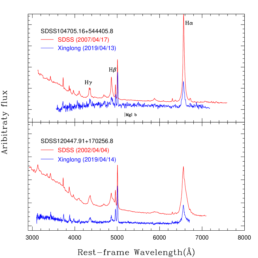
Figure 1: Comparison between the Xinglong spectra and the spectra extracted from the SDSS DR7 archive database. The SDSS spectra are convolved with a Gaussian profile to give a spectral resolution being identical to that of the Xinglong spectra. For each object, the two spectra are scaled to have a common flux of the total [O III]$\lambda$5007 line flux. All the spectra are transformed to the rest-frame, and are shifted vertically by an arbitrary amount for visibility. The fist three Balmer lines, H$\alpha$ (6563Å), H$\beta$ (4861Å) and H$\gamma$ (4340Å), are labeled on the upper panel.

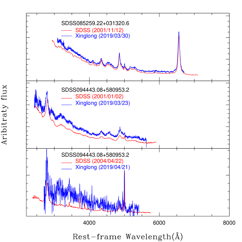
Figure 2: The same as in Figure 1 but for the other three non-CLQs.

4 Spectral Analysis

A spectral analysis is performed by following Wang et al. (2018, and references therein) in this section to shed a light on the turn-off type transitions occurring in the two CLQs.

4.1 AGN Continuum and Stellar Feature Removal

We at first model the continuum of each of the four spectra by a linear combination of the following components: (1) an AGN’s powerlaw continuum; (2) an template of both high-order Balmer emission lines and a Balmer continuum from the BLR; (3) an template of both optical and ultraviolet Fe II complex; (4) a host galaxy template with an age of 5Gyr extracted from the single stellar population (SSP) spectral library given in Bruzual & Charlot (2003); (5) an intrinsic extinction due to the host galaxy described by a galactic extinction curve with $R_{V}=3.1$. We use the empirical optical Fe II template provided by Veron-Cetty et al. (2004) and the theoretical template by Bruhweiler & Verner (2008) to model the optical and ultraviolet Fe II complex, respectively. The line width of the template is fixed in advance to be that of the broad component of H$\beta$, which is determined by our line profile modeling (see below).

The emission from a partially optically thick cloud with an electron temperature of $T_{e}=1.0\times 10^{4}$K is adopted to model the Balmer continuum $f_{\lambda}^{\mathrm{BC}}$ by following Dietrich et al. (2002, see also in Grandi 1982 and Malkan & Sargent 1982):

$$f_{\lambda}^{\mathrm{BC}}=f_{\lambda}^{\mathrm{BE}}B_{\lambda}(T_{e})(1-e^{-\tau}),\ \lambda\leq\lambda_{\mathrm{BE}}$$ (1)

where $f_{\lambda}^{\mathrm{BE}}$ is the continuum flux at the Balmer edge $\lambda_{\mathrm{BE}}=3646$Åand $B_{\lambda}(T_{e})$ is the Planck function. $\tau_{\lambda}$ is the optical depth at wavelength $\lambda$, which is related to the one at the Balmer edge $\tau_{\mathrm{BE}}$ as $\tau_{\lambda}=\tau_{\mathrm{BE}}(\lambda/\lambda_{\mathrm{BE}})^{3}$. A typical value of $\tau_{\mathrm{BE}}=0.5$ is adopted in our modeling of the continuum.

We model the high-order Balmer lines (i.e., H7-H50) by the case B recombination model with an electron temperature of $T_{e}=1.5\times 10^{4}$K and an electron density of $n_{e}=10^{8-10}\ \mathrm{cm^{-3}}$ (Storey & Hummer 1995). The widths of these high-order Balmer lines are, again, determined in advance according to the line profile modeling of the H$\beta$ broad emission (see below).

A $\chi^{2}$ minimization is performed iteratively over the whole spectroscopic wavelength range, except for the regions with known emission lines (e.g., H$\alpha$, H$\beta$, H$\gamma$, H$\delta$, [S II]$\lambda\lambda 6716,6731$, [N II]$\lambda\lambda 6548,6583$, [O I]$\lambda$6300, [O III]$\lambda\lambda 4959,5007$, [O II]$\lambda 3727$, [Ne III]$\lambda 3869$, and [Ne V]$\lambda$3426). For both SDSS spectra being typical of a type-I AGN, the underlying stellar emission is failed to be modeled because the continuum is entirely dominated by the AGN’s featureless emission. The modeling of the underlying stellar emission is also failed in the Xinglong spectrum of SDSS J1204+1702 due to the poor S/N ratio of its continuum. In contrast, the Xinglong spectrum of SDSS J1047+5444 shows a continuum being typical of an intermediate-type AGN with weak or negligible emission from the central engine, although our modeling based on a 5Gyr old SSP returns a poor reproduction of the continuum. In addition, our modeling suggests that the optical Fe II complex is too weak to be modeled in all the four spectra. The removal of the modeled continuum is illustrated in Figure 3 for the four spectra.

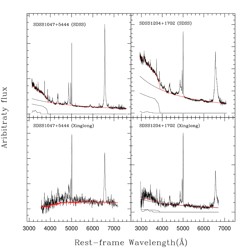
Figure 3: Illustration of the modeling and removal of the continuum for the SDSS DR7 and Xinglong spectra. In each panel, the top, heavy curve shows the observed rest-frame spectrum overplotted by the best-fitted continuum shown by the red curve. The light curves underneath show the individual components used in the modeling.

4.2 Line Profile Modeling

For each emission-line-isolated spectrum, the emission line profiles are modeled on both H$\alpha$ and H$\beta$ regions by the SPECFIT task (Kriss 1994) in the IRAF package.

In the profile modeling, each emission line is reproduced by a set of Gaussian profiles. By taking the poor continuum removal described above into account, a local linear continuum is additionally used for the Xinglong spectrum of SDSS J1047+5444 to reproduce the line profiles in the H$\beta$ region. The line flux ratios of the [O III]$\lambda\lambda$4959, 5007 and [N II]$\lambda\lambda$6548, 6583 doublets are fixed to their theoretical values, i.e., 1:3. The line widths of both H$\alpha$ and H$\beta$ broad components are measured directly on the residual profiles by the SPLOT task in the IRAF package after subtracting the modeled narrow components from the observed profiles. The line modelings are shown in the left and right panels of Figure 4 for the H$\beta$ and H$\alpha$ regions, respectively. The results of the profile modeling are listed in Table 2. No intrinsic extinction correction is applied to all the derived line fluxes, because the Balmer decrements of the narrow components determined from the SDSS spectra are as small as $\mathrm{H\alpha/H\beta}=2.87\pm 0.17$ and $1.43\pm 0.14$ for SDSS J1047+5444 and SDSS J1204+1702, respectively. All the errors reported in the table correspond to the 1$\sigma$ significance level after taking into account the proper error propagation.

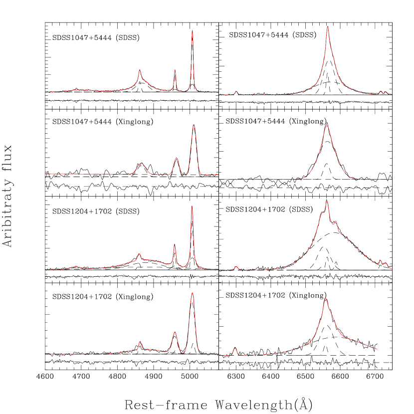
Figure 4: Line profile modelings by a linear combination of a set of Gaussian functions for the H$\beta$ (the left panels) and H$\alpha$ (the right panels) regions. In each panel the modeled continuum has already been removed from the original observed spectrum. The observed and modeled line profiles are plotted by black and red solid lines, respectively. Each Gaussian function is shown by a dashed line. The sub-panel underneath the line spectrum presents the residuals between the observed and modeled profiles.

Table 2: Spectral measurements and analysis.

SDSS ID	Epoch	AGN type	$F(\mathrm{[OIII]\lambda 5007})$	$F(\mathrm{H\beta_{b}})$	FWHM(H$\beta_{\mathrm{b}}$)	$F(\mathrm{H\alpha_{b}})$	FWHM(H$\alpha_{\mathrm{b}}$)	$M_{\mathrm{BH}}/M_{\odot}$	$L_{\mathrm{bol}}/L_{\mathrm{Edd}}$
			$\mathrm{10^{-15}\ erg\ s^{-1}\ cm^{-2}}$		$\mathrm{km\ s^{-1}}$	$\mathrm{10^{-15}\ erg\ s^{-1}\ cm^{-2}}$	$\mathrm{km\ s^{-1}}$
(1)	(2)	(3)	(4)	(5)	(6)	(7)	(8)	(9)	(10)
J1047+5444	2002/04/04	1.0	$13.5\pm 0.02$	$24.5\pm 1.1$	$2600\pm 120$	$102.5\pm 1.1$	$1970\pm 80$	$4.0\times 10^{7}$	0.41
	2019/04/14	1.9	$9.1\pm 0.2$			$18.7\pm 0.4$	$2940\pm 60$	$3.6\times 10^{7}$	0.15
J1204+1702	2007/04/17	1.0	$15.2\pm 0.3$	$40.0\pm 1.8$	$6720\pm 200$	$115.5\pm 1.0$	$4920\pm 50$	$3.7\times 10^{8}$	0.09
	2019/04/14	1.8/1.9	$14.7\pm 0.9$	$7.1\pm 0.4$	$6810\pm 600$	$35.7\pm 1.0$	$3140\pm 130$	$1.0\times 10^{8}$	0.12

4.3 Blackhole mass and Eddington ratio

Based on the line profile modelings, the SMBH viral mass ($M_{\mathrm{BH}}$) and Eddington ratio $L_{\mathrm{bol}}/L_{\mathrm{Edd}}$ (where $L_{\mathrm{Edd}}=1.26\times 10^{38}M_{\mathrm{BH}}/M_{\odot}\ \mathrm{erg\ s^{-1}}$ is the Eddington luminosity) are estimated for the two CLQs from the single-epoch spectroscopy through several well-established calibrated relationships (e.g., Wu et al. 2004; Kaspi et al. 2000, 2005; Peterson & Bentz 2006; Marziani & Sulentic 2012; Du et al. 2014, 2015; Peterson 2014; Wang et al. 2014).

Our estimations of both $M_{\mathrm{BH}}$ and $L_{\mathrm{bol}}/L_{\mathrm{Edd}}$ are based on the modeled broad H$\alpha$ emission lines. Green & Ho (2005) provided a calibration of

$$M_{\mathrm{BH}}=3.0\times 10^{6}\bigg{(}\frac{L_{\mathrm{H\alpha}}}{10^{42}\ \mathrm{erg\ s^{-1}}}\bigg{)}^{0.45}\bigg{(}\frac{\mathrm{FWHM(H\alpha)}}{1000\ \mathrm{km\ s^{-1}}}\bigg{)}^{2.06}M_{\odot}$$ (2)

to estimate $M_{\mathrm{BH}}$. To obtain an estimation of $L_{\mathrm{bol}}/L_{\mathrm{Edd}}$, we derive the bolometric luminosity $L_{\mathrm{bol}}$ from the standard bolometric correction $L_{\mathrm{bol}}=9\lambda L_{\lambda}(5100\AA)$ (e.g., Kaspi et al. 2000), where $L_{\lambda}(5100\AA)$ is the AGN’s specific continuum luminosity at 5100Å, which can be inferred from the H$\alpha$ broad-line luminosity through the calibration (Greene & Ho 2005)

$$\lambda L_{\lambda}(5100\AA)=2.4\times 10^{43}\bigg{(}\frac{L_{\mathrm{H\alpha}}}{10^{42}\ \mathrm{erg\ s^{-1}}}\bigg{)}^{0.86}$$ (3)

The estimated $M_{\mathrm{BH}}$ and $L_{\mathrm{bol}}/L_{\mathrm{Edd}}$ are tabulated in the Column (9) and (10) in Table 2, respectively. For each object, the used H$\alpha$ line flux measured from the Xinglong spectrum is scaled by a factor determined by equaling the total [O III]$\lambda 5007$ line flux to that of the corresponding SDSS spectroscopy.

For SDSS J1047+5444, the two spectra taken at different epochs return consistent estimations of the $M_{\mathrm{BH}}$. The corresponding $L/L_{\mathrm{Edd}}$ decreases from 0.41 to 0.15. For SDSS J1204+1702, we, however, obtain a roughly constant $L/L_{\mathrm{Edd}}$ when the object is at the “on” and “off” states. We argue that the invariable $L/L_{\mathrm{Edd}}$ is due to the difference in the estimated $M_{\mathrm{BH}}$, in which the $M_{\mathrm{BH}}$ determined from the SDSS spectrum is about four times larger than that from the Xinglong spectrum. By adopting the $M_{\mathrm{BH}}$ from the SDSS spectrum, similar as in SDSS J1047+5444, the corresponding $L/L_{\mathrm{Edd}}$ in fact decreases from 0.09 to 0.02.

5 Conclusion and Discussion

By performing a follow-up spectroscopy on five CL-AGN candidates recently selected by Macleod et al. (2019), we identify two new CL quasars, i.e., SDSS J1047+5444 and SDSS J1204+1702, both with a “turn-off” type transition, when the new spectra taken by the 2.16m telescope in Xinglong observatory are compared to the SDSS archival spectra.

With the increasing number of the identified CL-AGNs, there is accumulating evidence supporting that the change of SMBH’s accretion rate is the physical origin of the CL phenomenon (e.g., LaMass et al. 2015; Ruan et al. 2016; Runnoe et al. 2016; Gezari et al. 2017; Yang et al. 2018; Sheng et al. 2017; Wang et al. 2018; Yan et al. 2019; Macleod et al. 2016, 2019). The multi-wavelength light curves of the two newly identified CL-AGNs are plotted in Figure 5. Both objects show a continual decrease of the mid-infrared (MIR) brightness detected by the Wide-field Infrared Survey Explorer (WISE and NEOWISE-R, Wright et al. 2010; Mainzer et al. 2014) from 2010 to 2017, i.e., within the two spectroscopic epochs . The fading of the MIR emission supports the fact that the identified “turn-off” type transitions in the two objects are more likely due to the decrease of accretion rate rather than obscuring, because the MIR emission is mainly resulted from AGN-heated hot-dust which is less sensitive to dust obscuring (e.g., Sheng et al. 2017; Stern et al. 2018). Macleod et al. (2019) recently argued that the CLQs are the extreme tail of regular quasar variability (e.g, Rumbaugh et al. 2018). The argument is based on the fact that the CLQs are found to have relatively low $L/L_{\mathrm{Edd}}$, which is consistent with the well-known anti-correlation between $L/L_{\mathrm{Edd}}$ and variability amplitude previously revealed in quasars (e.g., Wilhite et al. 2008; Mao et al. 2009; Macleod et al. 2010).

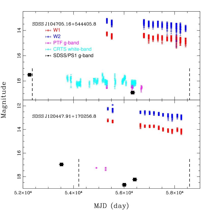
Figure 5: The multi-wavelength light curves for the two newly identified CL-AGNs. In each panel, the two vertical dashed lines mark the epochs of the SDSS and Xinglong spectra.

We compile a sample of 26 previously identified CL-AGNs from literature by requiring the detailed measurements on their both on and off states are provided in literature. Figure 6 shows the distributions of the CL-AGNs on the $L_{\mathrm{bol}}$ versus $M_{\mathrm{BH}}$ (the left panel) and $L_{\mathrm{bol}}$ versus $L/L_{\mathrm{Edd}}$ (the right panel) diagrams. The on and off states are plotted in the diagrams by the open and solid squares for each CL-AGN, respectively. The measurements given in Shen et al. (2011) and Chen et al. (2018) are adopted for the on state for each of the objects. For the off state, the value of $L_{\mathrm{bol}}$ is obtained from the corresponding value at the on state by a scaling factor determined through the change of the broad H$\alpha$ line flux. The comparison samples used in the diagrams include 1) the SDSS DR7 quasars with $z<0.5$ (Shen et al. 2011); 2) the SDSS DR3 narrow-line Seyfert 1 galaxies given in Zhou et al. (2006); 3) the Swift/BAT AGN sample with a spectral type classification in Winter et al. (2012); and 4) the SDSS intermediate-type Seyfert galaxies studied in Wang (2015).

Two facts can be learned from the comparison shown in Figure 6. On the one hand, as being consistent with Macleod et al. (2019), one can see from the figures that the CL-AGNs at on state are biased towards both low $L_{\mathrm{bol}}$ and low $L/L_{\mathrm{Edd}}$. This bias in fact motivates Macleod et al. (2019) to argue that the disk-wind BLR models proposed in Elitzur & Ho (2012) and Nicastro (2000) are plausible for understanding the (dis)appearance of the broad emission lines observed in the CL phenomenon, although a critical value of $L/L_{\mathrm{Edd}}\sim 10^{-3}$ is required for the (dis)appearance when the fiducal values of a set of parameters of the disk are adopted. On the other hand, there is an overlap between the intermediate-type AGNs and the CL-AGNs at their off state. By adopting the change of accretion rate as the physical origin of the CL phenomenon, this overlap strongly implies that the so-called intermediate-type AGNs are composed of two populations. One is due to the well-accepted orientation effect, and the another the intrinsic change of accretion rate, even though the physical origin of the change is still unclear at the current stage. In fact, the analysis of the X-ray spectra in Winter et al. (2012) suggests that the Seyfert-1.5 galaxies statistically show higher neutral column densities than the Seyfert 1 galaxies, which agrees with the expectation of the unified model (e.g., Antonucci 1993). The statistics in Figure 6 suggests that the two populations might differ from each other in $L_{\mathrm{bol}}$.

The expected timescale is still an open issue in the scenario of change of SMBH’s accretion rate (i.e., the viscosity crisis, e.g., Lawrence 2018 and references therein). The viscous timescale of a viscous radial inflow is expected to be (e.g., Krolik 1999; Shakura & Sunyaev 1973; LaMassa et al. 2015; Gezari et al. 2017)

$$\footnotesize t_{\mathrm{infl}}=6.5\bigg{(}\frac{\alpha}{0.1}\bigg{)}^{-1}\bigg{(}\frac{L/L_{\mathrm{Edd}}}{0.1}\bigg{)}^{-2}\bigg{(}\frac{\eta}{0.1}\bigg{)}^{2}\bigg{(}\frac{r}{10r_{g}}\bigg{)}^{7/2}\bigg{(}\frac{M_{\mathrm{BH}}}{1\times 10^{8}M_{\odot}}\bigg{)}\ \mathrm{yr}$$ (4)

where $\alpha$ is the “viscosity” parameter, $\eta$ is the efficiency of converting potential energy to radiation, and $r_{g}$ is the gravitational radius in unit of $GM/c^{2}$. Adopting $\alpha=\eta=L/L_{\mathrm{Edd}}=0.1$ and $M_{\mathrm{BH}}=1\times 10^{8}M_{\odot}$ yields a viscous timescale being comparable to the observations for the near-ultraviolet emission radiated from inner accretion disk with $r\sim 10r_{g}$. The timescale, however, dramatically increase to $\sim 10^{3}$yr for the optical emission coming from the outer disk with $r\sim 50-100r_{g}$.

Some solutions have been proposed to alleviate the timescale crisis. One solution is to involve the local disk thermal instability. The evolutionary $\alpha$-disk model developed in Siemiginowska et al. (1996) predicts a thermal timescale of

$$t_{\mathrm{th}}=2.7\bigg{(}\frac{\alpha}{0.1}\bigg{)}^{-1}\bigg{(}\frac{r}{10^{16}\ \mathrm{cm}}\bigg{)}^{3/2}\bigg{(}\frac{M_{\mathrm{BH}}}{10^{8}\ M_{\odot}}\bigg{)}^{1/2}\ \mathrm{yr}$$ (5)

Husemann et al. (2016) in fact reveals a temperature variation in Mrk 1018. The simulation carried out by Jiang et al. (2016) suggests that the development of the disk thermal instability favors low-metallicity gas. An alternative solution is to involve an accretion disk elevated by a magnetic field, which can results in a shorter variability timescale and can explain the CL phenomenon by an abrupt variation in magnetic torque (e.g., Ross et al. 2018; Stern et al. 2018; Dexter & Begelamn 2019).

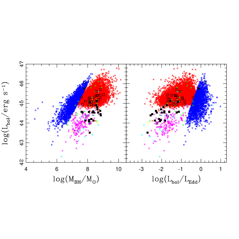
Figure 6: The distributions of the 26 previously identified CL-AGNs on the $L_{\mathrm{bol}}$-$M_{\mathrm{BH}}$ (the left panel) and $L_{\mathrm{bol}}$-$L_{\mathrm{bol}}/L_{\mathrm{Edd}}$ (the right panel) diagrams. The on and off states are denoted by the black open- and solid-squares, respectively. The used comparison samples are described as follows. Red cross: the quasars with $z<$0.5 taken from the value-added SDSS DR7 quasar catalog (Shen et al. 2011); blue cross: the SDSS DR3 NLS1 catalog established by Zhou et al. (2006); magenta cross: the SDSS DR7 intermediate-type AGNs studied in Wang (2015). The Swift/BAT AGN sample in Winter et al. (2012) is shown by the green, yellow and cyan cross for Seyfert 1, 1.2 and 1.5 galaxies, respectively.

The CL phenomenon is far from being understood at the current stage partially because of the limited CL-AGN sample size. Both repeat imaging and spectroscopy are necessary for expanding the sample size. Although some ongoing and forthcoming optical survey programs (e.g., Pan-STARRS1 survey, Chambers et al. (2016), Zwicky Transient Facility, Kulkarni (2018), All-Sky Automated Survey for Supernovae, Shappee et al. (2014), Large Synoptic Survey Telescope project, LSST Science Collaboration et al. (2017)), can provide many interesting targets for follow-up spectroscopy, how to flag the CL phenomenon efficiently by excluding the contamination caused by the AGN’s normal variation in optical bands is an open issue. This issue can be fairly addressed by some recently proposed space-based ultraviolet (UV) patrol missions (e.g., Wang et al. 2019; Sagiv et al. 2014; Mathew et al. 2018), because a significant variation in the AGN’s UV continuum is expected in the CL phenomenon. Additionally, a better understanding of the CL phenomenon can stem from the forthcoming larger time-domain spectroscopic surveys, for example the SDSS-V survey (Kollmeier et al. 2017).

References

- Antonucci (1993) Antonucci, R. R. J. 1993, ARA&A, 31, 473
- Bruhweiler & Verner (2008) Bruhweiler, F., & Verner, E. 2008, ApJ, 675, 83
- Bruzual & Charlot (2003) Bruzual, G., & Charlot, S. 2003, MNRAS, 344, 1000
- Cardelli et al. (1989) Cardelli, J. A., Clayton, G. C., & Mathis, J. S. 1989, ApJ, 345, 245
- Chambers etal. (2016) Chambers, K. C., Magnier, E. A., Metcalfe, N., et al. 2016, arXiv:astro-ph/1612.05560
- Chen et al. (2018) Chen, Z. F., Pan, D. S., Pang, T. T., & Huang, Y. 2018, ApJS, 234, 16
- Dietrich et al. (2003) Dietrich, M., Hamann, F., Shields, J. C., et al. 2002, ApJ, 581, 912
- Dexter & Begelamn (2019) Dexter, J., & Begelman, M. C. 2019, MNRAS, 483, L17
- Du et al. (2015) Du, P., Hu, C., Lu, K. X., et al. 2015, ApJ, 806, 22
- Du et al. (2014) Du, P., Wang, J. M., Hu, C., Valls-Gabaud, D., Baldwin, J, A., Ge, J. Q., & Xue, S. J. 2014, MNRAS, 438, 2828
- Elitzur & Ho (2009) Elitzur, M., & Ho, L. C. 2009, ApJ, 701, 91
- Elitzur et al. (2014) Elitzur, M., Ho, L. C., & Trump, J. R. 2014, MNRAS, 438, 3340
- Fan et al. (2016) Fan, Z., Wang, H. J., Jiang, X. J., et al. 2016, PASP, 128, 115005
- Frederick et al. (2019) Frederick, S., Gezari, S., Graham, M. J., et al. 2019, arXiv:astro-ph/1904.10973
- Gezari et al. (2017) Gezari, S., Hung, T., Cenko, S. B., et al. 2017, ApJ, 835, 144
- Grandi (1982) Grandi, S. A. 1982, ApJ, 255, 25
- Greene & Ho (2005) Greene, J. E., & Ho, L. C. 2005, ApJ, 630 ,122
- Husemann et al. (2016) Husemann, B., Urrutia, T., Tremblay, G. R., et al. 2016, A&A, 593, L9
- Jiang et al. (2016) Jiang, Y. F., Davis, S. W., & Stone, J. M. 2016, ApJ, 827, 10
- Kaspi et al. (2005) Kaspi, S., Maoz, D., Netzer, H., Peterson, B. M., Vestergaard, M., & Jannuzi, B. T. 2005, ApJ, 629, 61
- Kaspi et al. (2000) Kaspi, S., Smith, P.S., Netzer, H., Maoz, D., Jannuzi, B.T., & Giveon, U. 2000, ApJ, 533, 631
- Kollmeier et al. (2017) Kollmeier, J. A., Zasowski, G., Rix, H. W., et al. 2017, arXiv: astro-ph/1711.03234
- Kriss (1994) Kriss, G. 1994, Adass, 3, 437
- Kulkarni (2018) Kulkarni, S. R. 2018, ATel, 11266, 1
- LaMassa et al. (2015) LaMassa, S. M., Cales, S., Moran, E. C., et al. 2015, ApJ, 800, 144
- Lawrence (2018) Lawrence, A. 2018, Nature Astronomy, 2, 102
- LSST Science Collaboratio (2017) LSST Science Collaboration 2017, arXiv:astro-ph/1708.04058
- MacLeod et al. (2019) MacLeod, C. L., Green, P. J., Anderson, S. F., et al. 2019, ApJ, 874, 8
- MacLeod et al. (2016) MacLeod, C. L., Ross, N. P., Lawrence, A., et al. 2016, MNRAS, 457, 389
- MacLeod et al. (2010) MacLeod, C. L., Ivezic, Z., Kochanek, C. S., et al. 2010, ApJ, 721, 1014
- Malkan & Sargent (1982) Malkan, M. A., & Sargent, W. L. W. 1982, ApJ, 254, 22
- Mao et al. (2009) Mao, Y. F., Wang, J., & Wei, J. Y. 2009, RAA, 9, 529
- Mainzer et al. (2014) Mainzer, A., Bauer, J., Cutri, R. M., et al. 2014, ApJ, 792, 30
- Massey et al. (1988) Massey, P., Strobel, K., Barnes, J. V., et al. 1988, ApJ, 328, 315
- Mathew et al. (2018) Mathew, J., Ambily, S., Prakash, A., et al. 2018, ExA., 45, 201
- Matt et al. (2003) Matt, G., Guainazzi, M., & Maiolino, R. 2003, MNRAS, 342, 422
- McElroy et al. (2016) McElroy, R. E., Husemann, B., Croom, S. M., et al. 2016, A&A, 593, L8
- Nicastro (2000) Nicastro, F. 2000, ApJ, 530, 65
- Peterson (2014) Peterson, B. M. 2014, SSRv, 183, 253
- Peterson & Bentz (2006) Peterson, B. M., & Bentz, M. C. 2006, New A Rev., 50, 769
- Peterson & Perez (1984) Penston, M. V., & Perez, E. 1984, MNRAS, 211, 33
- Piconcelli et al. (2007) Piconcelli, E., Fiore, F., Nicastro, F., Mathur, S., Brusa, M., Comastri, A., & Puccetti, S. 2007, A&A, 473, 85
- Ricci et al. (2016) Ricci, C., Bauer, F. E., Arevalo, P., et al. 2016, ApJ, 820, 5
- Risaliti et al. (2009) Risaliti, G., Salvati, M., Elvis, M., et al. 2009, MNRAS, 393, L1
- Ruan et al. (2016) Ruan, J. J., Anderson, S. F., Cales, S. L., et al. 2016, ApJ, 826, 188
- Ross et al. (2018) Ross, N. P., Ford, K. E. S., Graham, M., et al. 2018, MNRAS, 480, 4468
- Rumbaugh et al. (2018) Rumbaugh, N., Shen, Y., Morganson, E., et al. 2018, ApJ, 854, 160
- Runnoe et al. (2016) Runnoe, J. C., Cales, S., Ruan, J. J., et al. 2016, MNRAS, 455, 1691
- Sagiv et al. (2014) Sagiv, I., Gal-Yam, A., Ofek, E. O., et al. 2014, AJ, 147, 79
- Shakura & Sunyaev (1973) Shakura, N. I., & Sunyaev, R. A. 1973, A&A, 24, 337
- Schlafly & Finkbeiner (2011) Schlafly, E. F., & Finkbeiner, D. P. 2011, ApJ, 737, 103
- Shapovalova et al. (2010) Shapovalova, A. I., Popovic, L. C., Burenkov, A. N., et al. 2010, A&A, 509, 106
- Shappee et al. (2014a) Shappee, B. J., Prieto, J. L., Grupe, D., et al. 2014a, ApJ, 788, 48
- Shappee et al. (2014b) Shappee, B., Prieto, J., Stanek, K. Z., et al. 2014b, AAS, 223, 23603
- Shen & Ho (2014) Shen, Y., & Ho, Luis C. 2014, Nature, 513, 210
- Shen et al. (2011) Shen, Y., Richards, G. T., Strauss, M. A., et al. 2011, ApJS, 194, 45
- Sheng et al. (2017) Sheng, Z., Wang, T., Jiang, N., et al. 2017, ApJ, 846, 7
- Siemiginowska et al. (1996) Siemiginowska, A., Czerny, B., & Kostyunin, V. 1996, ApJ, 458, 491
- Stern et al. (2018) Stern, D., McKernan, B., Graham, M. J., et al. 2018, ApJ, 864, 27
- Storey & Hamann (1995) Storey, P. J., & Hummer, D. G. 1995, MNRAS, 272, 41
- Trakhtenbrot et al. (2019) Trakhtenbrot, B., Arcavi, I., MacLeod, C. L., et al. 2019, arXiv:astro-ph/1903.11084
- Tody (1986) Tody, D. 1986, SPIE, 627, 733
- Tody (1993) Tody, D. 1992, ASPC, 52, 173
- Veron-Cetty et al. (2004) Veron-Cetty, M.-P., Joly, M., & Veron, P. 2004, A&A, 417, 515
- Wang (2015) Wang, J. 2015, New A, 37, 15
- Wang et al. (2019) Wang, J., Liang, E. W., & Wei, J. Y. 2019, accepted by PASP, arXiv: astro-ph/1906.03375
- Wang et al. (2018) Wang, J., Xu, D. W., & Wei, J. Y. 2018, ApJ, 858, 49
- Wang et al. (2014) Wang, J. M., Du, P., Hu, C., et al. 2014, ApJ, 793, 108
- Wilhite et al. (2008) Wilhite, B. C., Brunner, R. J., Grier, C. J., Schneider, D. P., & vanden Berk, D. E. 2008, MNRAS, 383, 1232
- Winter et al. (2012) Winter, L. M., Veilleux, S., McKernan, B., & Kallman, T. R. 2012, ApJ, 745, 107
- Wright et al. (2010) Wright, E. L., Eisenhardt, P. R. M., Mainzer, A. K., et al. 2010, AJ, 140, 1868
- Wu et al. (2004) Wu, X. B., Wang, R., Kong, M. Z., Liu, F. K., & Han, J. L. 2004, A&A, 424, 793
- Yan et al. (2019) Yan, L., Wang, T. G., Jiang, N., et al. 2019, ApJ, 874, 44
- Yang et al. (2017) Yang, Q., Wu, X. B., Fan, X. H., et al. 2018, ApJ, 862, 109
- Zhou et al. (2006) Zhou, H. Y., Wang, T. G., Yuan, W. M., Lu, H. L., Dong, X. B., Wang, J. X., & Lu, Y. J. 2006, ApJS, 166, 128