Correlated nonequilibrium steady states without energy flux

Abstract

Floquet engineering of closed quantum systems can lead to the formation of long-lived prethermal states that, in general, eventually thermalize to infinite temperature. Coupling these driven systems to dissipative baths can stabilize such states, establishing a true nonequilibrium steady state. We demonstrate that in a certain strongly interacting lattice model coupled to a bath and driven by an electric field, such steady states can have the remarkable property that the cycle-averaged rate of energy transfer between the lattice and the baths vanishes. Despite this, we show that these states retain a clear nonequilibrium nature.

I Introduction

Closed, interacting quantum systems driven by a time-dependent external field are generically expected to absorb energy from the field and evolve towards an infinite temperature state.(Rigol et al., 2008) However, in certain cases they can be trapped in a nonequilibrium prethermal state (Bukov et al., 2015, 2016; Herrmann et al., 2017; Weidinger and Knap, 2017) that is long-lived, but not permanent.(D’Alessio and Rigol, 2014) In contrast, in cases ranging from, e.g., a single particle in a double well (Grossmann et al., 1991) or lattice (Dunlap and Kenkre, 1986) to discrete few-state models (Großmann and Hänggi, 1992) and systems of noninteracting particles,(Čadež et al., 2017) periodic fields can lead to complete dynamical localization or coherent destruction of coupling such that special Floquet states can survive indefinitely.

Many-body localized systems (Gornyi et al., 2005; Basko et al., 2006) are perhaps the only known example of extended, isolated and interacting systems that do not absorb heat when driven by a periodic potential .(Ponte et al., 2015) The signatures of many-body localized phases can even survive the introduction of phonons when driven.(Lenarčič et al., 2018, 2019) However, localization is known to be fragile (D’Alessio and Rigol, 2014) and is rapidly destroyed in the presence of generic small perturbations.(Luitz et al., 2017) Recent experimental progress in, e.g. ultrafast optical manipulation of solids (Först et al., 2011) and control of ultracold atomic gases (Gross and Bloch, 2017) has brought these questions, and periodically driven many-body systems in general, to the forefront of present-day scientific discussion.(Moessner and Sondhi, 2017; Bordia et al., 2017; Reitter et al., 2017; Pomarico et al., 2017; Messer et al., 2018; Roy et al., 2018; Werner et al., 2019)

Real systems are never perfectly isolated. Open quantum systems can dissipate absorbed energy into baths, and therefore typically reach a nonequilibrium steady state (NESS) depending on the properties of both the coupling to the bath and the drive.(Weiss, 1999) A dissipative bath allows for stabilization of nonthermal Floquet states in nonintegrable many-body lattice models.(Tsuji et al., 2009; Murakami et al., 2017; Murakami and Werner, 2018; Peronaci et al., 2018) At NESS, heating still occurs, but the rate at which energy is absorbed from the field is equal to the rate at which it is dissipated to the bath.

With a few recent exceptions,(Murakami et al., 2017; Murakami and Werner, 2018; Qin and Hofstetter, 2018) the rate of energy dissipation into the bath from many-body lattice systems driven into periodic NESS has been largely unexplored. We present a case where this rate, averaged over time, appears to be either zero or negligibly small. Notably, maintaining the nonequilibrium state in the model considered here does require a constant absorption of energy, which must then be dissipated. However, even though the lattice is driven, energy is absorbed and dissipated entirely by the baths (which are also driven for reasons explained below). Within any single field cycle, the amount of energy flowing out of the lattice is exactly balanced by the amount flowing into it.

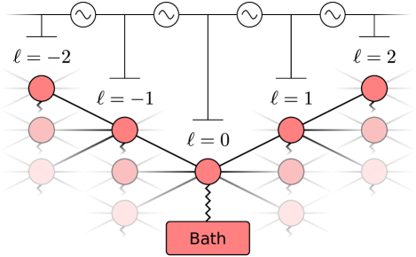
Figure 1: Model: sites on a Bethe lattice are divided into layers, and coupled to the sites in adjacent layers and to baths. A time-dependent potential difference $\Delta\phi\left(t\right)$ is applied between consecutive layers, driving a current within the lattice.

II Model

We consider a system for which exact dynamics can be obtained by numerical methods, though the present treatment will be approximate: a Hubbard model on a Bethe lattice of coordination number $Z$, at the infinite $Z$ limit, driven by an oscillating electric field and in contact with a set of noninteracting metallic baths (see Fig. 1). Each bath is coupled to a single lattice site and held at the same potential as that site (bath sites are therefore necessarily driven). The system’s Hamiltonian is

$$\hat{H}=\hat{H}_{L}+\hat{H}_{B}+\hat{H}_{LB}.$$ (1)

Here, the particle–hole symmetric lattice Hamiltonian $\hat{H}_{L}$ and bath Hamiltonian $\hat{H}_{B}$ are given by

$$\hat{H}_{L}\left(t\right) =-J\sum_{\left\langle ij\right\rangle\sigma}\hat{d}_{i\sigma}^{\dagger}\hat{d}_{j\sigma}+\sum_{i,\sigma}\phi_{i}\left(t\right)\hat{n}_{i\sigma}$$ (2)

$$+U\sum_{i}\left(\hat{n}_{i\uparrow}-\frac{1}{2}\right)\left(\hat{n}_{i\downarrow}-\frac{1}{2}\right),$$

$$\hat{H}_{B} =\sum_{ik\sigma}\left(\varepsilon_{k}+\phi_{i}\left(t\right)\right)\hat{b}_{ik\sigma}^{\dagger}\hat{b}_{ik\sigma}.$$

The $\hat{d}_{i\sigma}$ and $\hat{d}_{i\sigma}^{\dagger}$, respectively, are fermionic annihilation and creation operators on the lattice and $\hat{n}_{i\sigma}=\hat{d}_{i\sigma}^{\dagger}\hat{d}_{i\sigma}$. The $\hat{b}_{ik\sigma}$ and $\hat{b}_{ik\sigma}^{\dagger}$ are a corresponding set of fermionic operators within the noninteracting bath attached to lattice site $i$. $J\equiv\frac{t_{0}}{\sqrt{Z}}$ is the lattice hopping amplitude $t_{0}$ scaled by the coordination number and $U$ is the Hubbard interaction strength. We set $t_{0}\equiv 1$ and employ it as our unit of energy, also setting $\hbar\equiv 1$. The system is subjected to an oscillating electric potential $\phi_{i}\left(t\right)$, and the $\varepsilon_{k}$ are single-particle energies within the baths.

The final term in the Hamiltonian describes the lattice–bath coupling, and is given by

$$\hat{H}_{LB}=\sum_{ik\sigma}\left(V_{k}\hat{b}_{ik\sigma}^{\dagger}\hat{d}_{i\sigma}+h.c.\right).$$ (3)

The $V_{k}$ are chosen for numerical convenience so as to generate a flat density of states $\Gamma_{i}\left(\omega\right)=\sum_{k}\left|V_{k}^{2}\right|\delta\left(\omega-\varepsilon_{k}\right)=\frac{\Gamma}{\left(1+e^{\nu\left(\omega-\omega_{c}\right)}\right)\left(1+e^{-\nu\left(\omega+\omega_{c}\right)}\right)}$ with bandwidth $2\omega_{c}$ and edges softly falling off over an energy range $\frac{1}{\nu}$. We take $\omega_{c}=50$, $\nu=10$ (essentially the wide band limit) and $\Gamma=\frac{1}{2}$. We further set the baths’ inverse temperature to $\beta=1$ and their chemical potential $\mu$ to zero. We note that modeling the baths by Lindblad operators at this point would completely fail to capture the physics in which we are interested, because we will consider energy going back and forth between the lattice and baths; a non-Markovian description is therefore crucial.

To set up a nonequilibrium situation, the system is divided into layers labeled by an index $\ell$ such that each site in layer $\ell$ is connected to $\frac{Z}{2}$ neighbors in each of the layers $\ell\pm 1$, and $\phi_{i}=\ell_{i}E\cos\left(\varOmega t\right)$. We note that each lattice site is always at the same potential as its bath, as implied by the requirement that the bath describes a spatially adjacent metallic region. The potential difference between two consecutive layers is therefore $\Delta\phi\left(t\right)=\pm E\cos\left(\varOmega t\right)$, and drives an alternating current in the lattice. Fig. 1 illustrates this at $Z=6$; at $Z=2$ the system would simply be a 1D chain in a linear oscillating field. While $\phi_{i}\left(t\right)$ breaks translation symmetry, we follow other studies (Aoki et al., 2014) in employing a Peierls substitution to eliminate the potential terms from the Hamiltonian, shifting them to a site-independent phase in the hopping amplitudes. This is equivalent to a rotating frame transformation with respect to $\hat{R}\left(t\right)=e^{-i\sum_{i\sigma}\Phi_{i\sigma}\left(t\right)\left(\hat{n}_{i\sigma}+\sum_{k}\hat{b}_{ik\sigma}^{\dagger}\hat{b}_{ik\sigma}\right)}$, where $\Phi_{i\sigma}\left(t\right)=\int_{0}^{t}\phi_{i\sigma}\left(\tau\right)\mathrm{d\tau}=l_{i}A\sin(\varOmega t)$ and $A\equiv\frac{E}{\Omega}$ is a dimensionless driving amplitude.

III Numerical solution and observables

We evaluate the time evolution of the system within nonequilibrium dynamical mean field theory (DMFT), which is exact for models of this type at $Z\rightarrow\infty$.(Georges et al., 1996; Freericks et al., 2006; Aoki et al., 2014) DMFT maps the lattice model onto an effective impurity model, which we solve within strong coupling perturbation theory using the noncrossing approximation (NCA).(Bickers, 1987; Eckstein and Werner, 2010; Cohen et al., 2014a, b; Antipov et al., 2017) This approach is appropriate in the insulating regime, where the Coulomb interaction is strong compared to the lattice hopping, and is the only approximation used here. The lattice is initially assumed to be in an antiferromagnetic Néel state, and is coupled to the bath at time $t=0$. We evaluate the double occupation $d_{i}(t)=\left\langle\hat{n}_{i\uparrow}\left(t\right)\hat{n}_{i\downarrow}\left(t\right)\right\rangle$; the local Green’s functions $G_{\sigma}\left(t,t^{\prime}\right)=\left\langle\hat{d}_{i\sigma}\left(t\right)\hat{d}_{i\sigma}^{\dagger}\left(t^{\prime}\right)\right\rangle$; and the lattice–bath energy current

$$I_{E}(t) =-\frac{\mathrm{d}}{\mathrm{d}t}\left\langle\hat{H}_{B}\left(t\right)-\hat{H}_{B,\mathrm{internal}}\left(t\right)\right\rangle$$ (4)

$$=-i\sum_{ik\sigma}\varepsilon_{k}V_{k}\left\langle\hat{b}_{ik\sigma}^{\dagger}\hat{d}_{i\sigma}-\hat{d}_{i\sigma}^{\dagger}\hat{b}_{ik\sigma}\right\rangle.$$

The latter definition is given by the time derivative of the bath energy after removing the internal energy generation $\frac{\mathrm{d}}{\mathrm{d}t}\left\langle\hat{H}_{B,\mathrm{internal}}\left(t\right)\right\rangle=\sum_{i,k,\sigma}\dot{\phi_{i}}\left(t\right)\hat{b}_{ik\sigma}^{\dagger}\hat{b}_{ik\sigma}$. This term describes irreversibly dissipated energy, which will not be explored here.

We note that the model of Eq. (1) was used for theoretical convenience rather than experimental realizability. One could generalize the theoretical treatment to more realistic finite-dimensional lattices, at the cost that DMFT will no longer be exact. It would then further be possible, at the cost of greatly increased computational difficulty, to improve the theory by introducing nonlocal corrections to DMFT in any of a variety of established methods.(Maier et al., 2005; Rubtsov et al., 2008; Kananenka et al., 2015; Zgid and Gull, 2017) This goes beyond the scope of the present manuscript.

IV High frequency limit

Before considering numerical results, a qualitative understanding of the system can be obtained from analytical considerations. Bukov et al. Bukov et al., 2016 showed that that for periodic driving of period $T$ or equivalently frequency $\varOmega=\frac{2\pi}{T}$, such that $\hat{H}\left(t\right)=\hat{H}\left(T+t\right)$, an approximate static Hamiltonian $\hat{H}_{eff}$ can be derived at the high frequency limit (HFL) by way of a generalized Schrieffer–Wolff transformation and an expansion in $\frac{1}{\Omega}$. In the present model, the transformation can be performed by going to the rotating frame with respect to the operator $\hat{R}\left(t\right)=e^{-iUt\sum_{i}\left(\hat{n}_{i\uparrow}-\frac{1}{2}\right)\left(\hat{n}_{i\downarrow}-\frac{1}{2}\right)-i\sum_{i\sigma}\Phi_{i\sigma}\left(t\right)\left(\hat{n}_{i\sigma}+\sum_{k}\hat{b}_{ik\sigma}^{\dagger}\hat{b}_{ik\sigma}\right)}$. For resonant driving $U=l\varOmega$ with $l\in\mathcal{N}$, the leading-order effective Hamiltonian $\hat{H}_{\mathrm{eff}}^{\left(0\right)}=\frac{1}{T}\int_{0}^{T}\mathrm{d}t\hat{H}_{\mathrm{rot}}\left(t\right)$ then takes the simple form

$$\hat{H}_{\mathrm{eff}}^{\left(0\right)} =-J\sum_{\left\langle ij\right\rangle\sigma}\left[\mathcal{J}_{0}\hat{g}_{ij\sigma}+\left(\mathcal{J}_{l}\left(-1\right)^{l\eta_{ij}}\hat{h}_{ij\sigma}^{\dagger}+h.c.\right)\right]$$ (5)

$$-\frac{4i}{\pi}\sum_{ik\sigma}V_{k}\left[\hat{h}_{ik\sigma}^{\dagger}-h.c.\right].$$

Here, $\eta_{ij}=1$ for $i>j$ and $\eta_{ij}=0$ for $i<j$. $\mathcal{J}_{l}\equiv\mathcal{J}_{l}\left(A\right)$ denotes the $l^{\mathrm{th}}$ order Bessel function of the dimensionless driving amplitude $A=\frac{E}{\varOmega}$. The effective Hamiltonian within the lattice contains two types of operators with couplings set by $A$: the first is doublon and holon hopping, described by $\hat{g}_{ij\sigma}=\hat{n}_{i\bar{\sigma}}\hat{d}_{i\sigma}^{\dagger}\hat{d}_{j\sigma}\hat{n}_{j\bar{\sigma}}+\left(1-\hat{n}_{i\bar{\sigma}}\right)\hat{d}_{i\sigma}^{\dagger}\hat{d}_{j\sigma}\left(1-\hat{n}_{j\bar{\sigma}}\right)$; and the second is creation/annihilation of doublon–holon pairs, described respectively by $\hat{h}_{ij\sigma}^{\dagger}=\hat{n}_{i\bar{\sigma}}\hat{d}_{i\sigma}^{\dagger}\hat{d}_{j\sigma}\left(1-\hat{n}_{j\bar{\sigma}}\right)$ and its Hermitian conjugate $\hat{h}_{ij\sigma}$. Coupling to the bath introduces modified terms of the second type, given by $\hat{h}_{ik\sigma}^{\dagger}=\hat{b}_{ik\sigma}^{\dagger}\hat{d}_{i\sigma}\left(\hat{n}_{i\bar{\sigma}}-\frac{1}{2}\right)$ and $\hat{h}_{ik\sigma}$ and respectively denoting creation / annihilation of excitations associated with lattice–bath tunneling processes. The energy current operator, in the rotating frame and up to first order in the high frequency expansion, is $\hat{I}_{E,\mathrm{eff}}^{(0)}\left(t\right)=\frac{4}{\pi}\sum_{i,k,\sigma}\varepsilon_{k}V_{k}\left[\hat{h}_{ik\sigma}^{\dagger}+h.c.\right]$, and contains only doublon/holon density dependent hopping terms.

We make no particular claims regarding the accuracy of the HFL (corrections in the resonant case have been explored in the literature (Herrmann et al., 2017)), and our main results do not rely on taking this limit. Nevertheless, we show below that it captures the basic physical picture at a qualitative (but not quantitative) level.

We proceed by writing a master equation for the NESS occupation probabilities $P_{\alpha}$ of a lattice site. The index $\alpha$ refers to the four possible states of an isolated site, denoted by $\left|0\right\rangle$ (unoccupied), $\left|\sigma\right\rangle$ (singly occupied with $\sigma\in\left\{\uparrow,\downarrow\right\}$) and $\left|\uparrow\downarrow\right\rangle$ (doubly occupied). The static NESS must have no net flow in or out of any state, such that $\sum_{\beta}R_{\alpha\rightarrow\beta}P_{\alpha}=\sum_{\beta}R_{\beta\rightarrow\alpha}P_{\beta}.$ Given the rates $R_{\alpha\rightarrow\beta}$, the $P_{\alpha}$ can be obtained from this condition with the additional requirement of normalization, $\sum_{\alpha}P_{\alpha}=1$.

We estimate rates in the HFL by projecting Eq. 5 onto the subspace of a pair of adjacent lattice sites $i$ and $j$, $\left|n_{i}n_{j}\right\rangle$; and considering Golden rule transition rates between the different states. The expectation values of particle number operators $\hat{n}_{j\mathbf{\sigma}}$ or their products are then expressed in terms of local state probabilities, i.e. $\left\langle\hat{n}_{j\sigma}\right\rangle=P_{\left|\sigma\right\rangle_{j}}+P_{\left|\uparrow\downarrow\right\rangle_{j}}$. For example, the rate $R_{\left|\sigma\right\rangle\leftarrow\left|0\right\rangle}=-\mathcal{J}_{0}\left(A\right)P_{\left|\sigma\right\rangle}P_{\left|0\right\rangle}-\mathcal{J}_{l}\left(A\right)P_{\left|\uparrow\downarrow\right\rangle}P_{\left|0\right\rangle}$. To this, one must add the rates $R_{\left|0\right\rangle\leftarrow\left|\sigma\right\rangle}^{\mathrm{bath}}=R_{\left|\uparrow\downarrow\right\rangle\leftarrow\left|\sigma\right\rangle}^{\mathrm{bath}}=\frac{2\Gamma}{\pi^{2}}f$ and $R_{\left|\sigma\right\rangle\leftarrow\left|0\right\rangle}^{\mathrm{bath}}=R_{\left|\sigma\right\rangle\leftarrow\left|\uparrow\downarrow\right\rangle}^{\mathrm{bath}}=\frac{2\Gamma}{\pi^{2}}\left(1-f\right)$ for transitions mediated by tunneling of electrons between the lattice and bath, where $f=\frac{1}{1+e^{\beta\left(\varepsilon-\mu\right)}}$ is the bath Fermi function.

The rate equations can be further simplified by enforcing the symmetries $P_{\left|0\right\rangle}=P_{\left|\uparrow\downarrow\right\rangle}$ and $P_{\left|\sigma\right\rangle}=P_{\left|\bar{\sigma}\right\rangle}$, but remain cubic, and their solution is unwieldy. To gain more intuition, we linearize the equations by replacing the probabilities within the rates by their approximate values at large $U$: $P_{\left|\uparrow\downarrow\right\rangle}^{\mathrm{rate}}\simeq 0$ and $P_{\left|\sigma\right\rangle}^{\mathrm{rate}}\simeq\frac{1}{2}$. This finally yields the double occupation probability $d^{\mathrm{HFL}}$:

$$d^{\mathrm{HFL}}\equiv P_{\left|\uparrow\downarrow\right\rangle} =\frac{\pi^{2}\left|\mathcal{J}_{l}\left(A\right)\right|+4\left(1-f\right)}{8\left(\frac{\pi^{2}\left|\mathcal{J}_{l}\left(A\right)\right|}{4}+1\right)},$$ (6)

where $f$ is once again the bath Fermi function parameterized by $\beta=1$, $\mu=0$ and the transition energy $\varepsilon=5$. Within the steady state master equation, state $\alpha$ is occupied at probability $P_{\alpha}$ and a transition from it to state $\beta$, which occurs at rate $R_{\beta\leftarrow\alpha}^{\mathrm{bath}}$, contributes the energy difference $E_{\beta}-E_{\alpha}$ to the the energy flux. The lattice–bath energy current is therefore $I_{E}^{\mathrm{HFL}}=-\sum_{\beta}\left(E_{\beta}-E_{\alpha}\right)R_{\beta\leftarrow\alpha}^{\mathrm{bath}}P_{\alpha}$, with $E_{\alpha}$ the energy of the isolated state $\left|\alpha\right\rangle$. An analogous discussion for deriving the charge current can be found in Ref. Datta, 2005.

V Results

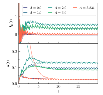
Figure 2: Energy current between the lattice and bath (upper panel) and double occupation (lower panel) within the NCA. The electric field’s frequency $\varOmega=U=10$ is set to resonance, and several field amplitudes $A$ are shown. Lighter lines denote an alternative initial condition (see text).

In Fig. 2, we plot the NCA dot–bath energy current $I_{E}(t)$ (upper panel) and double occupation $d\left(t\right)$ (lower panel), which show the numerical data extrapolated to $\Delta t\rightarrow 0$. Both quantities are shown at resonant driving $l=1$ (i.e. $\varOmega=U=10$) and at several field amplitudes $A$. In equilibrium ($A=0$), energy flows between the system and bath only for times $t\lesssim 2$, while the system is still relaxing to equilibrium with the bath after the initial quench. Activating the electric field induces oscillations in both observables. A stable NESS emerges at all amplitudes after a timescale $t\gtrsim 2\sim\frac{1}{\Gamma}$, and we have verified that doubling the final simulation time makes essentially no difference (not shown). At small amplitudes ($A=1,2$), $I_{E}(t)$ and $d\left(t\right)$ both grow with increasing $A$; however, at higher amplitudes ($A\gtrsim 3$) they decrease with increasing $A$, with a very strong suppression apparent at the first Bessel zero $A\approx 3.831$. Since the system is close to the Mott regime at $A=0$, an increase in $d(t)$ implies that energy from the field is absorbed by doublons and holons.

Floquet stabilization differs from dynamical decoupling in that the NESS is determined by the driving and dissipative coupling rather than the initial condition. To demonstrate this, lighter lines in Fig. 2 show, for two representative amplitudes, dynamics starting from a state where even(odd) lattice layers are doubly occupied(unoccupied). The doublon/holon occupation rapidly attains the same NESS to within numerical accuracy.

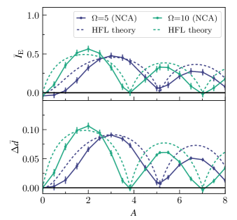
Figure 3: Amplitude dependence of the period averaged energy current $\bar{I}_{E}(A)$ (upper panel) and double occupation difference $\Delta\bar{d}(A)$ (lower panel, see text for definition). The driving frequencies shown are $\varOmega=U/2=5$ and $\varOmega=U=10$. NCA results are plotted as solid lines, while dashed lines denote values obtained from the HFL theory and multiplied by a factor of 50 to be visible on the same scale.

A simpler picture emerges if we consider NESS observables averaged over a driving cycle. For any observable $O$, we define $\bar{O}\equiv\frac{1}{T}\int_{t_{m}-T}^{t_{m}}\mathrm{d}t\thinspace O\left(t\right)$, where $t_{m}$ is the maximum simulation time. The upper panel of Fig. 3 then shows the NCA period averaged energy current $\bar{I}_{E}(A)$, at $\Omega=U$ ($l=1$) and at $\Omega=\frac{U}{2}$ $\left(l=2\right)$, as solid lines. The error bars denote numerical and finite-time uncertainties in our solution of the NCA equations. These are obtained by considering deviations from exact sum rules: for the energy current the error estimate is given by the difference of $\bar{I}_{E}\left(A=0\right)$ from zero, and for the double occupation by the deviation of the trace of the reduced density matrix in the atomic subspace from one. The lower panel shows $\varDelta\bar{d}(A)=\bar{d}(A)-\bar{d}(0)$, the difference between the period averaged double occupation $\bar{d}(A)$ and its equilibrium counterpart at $A=0$. Both $\bar{I}_{E}(A)$ and $\varDelta\bar{d}(A)$ have an amplitude dependence reminiscent of a Bessel function $\left|\mathcal{J}_{l}\left(A\right)\right|$, with $l$ set by the frequency. The similarity between $\bar{I}_{E}$ and $\bar{d}$ suggests that dissipation is mediated by the creation and destruction of holons and doublons. Remarkably, in the $l=1$ regime, tuning the dimensionless amplitude $A$ to Bessel zeros suppresses the creation of doublon–holon pairs and therefore the average rate of energy transfer between the lattice and the baths vanishes to within the numerical uncertainties. Fig. 3 demonstrates that for amplitudes with $A\approx 3.831,7.015$ a NESS is maintained such that within a cycle and within numerical uncertainties, no energy dissipation occurs. At $l=2$, finite dissipation is predicted, but it should be noted that the NCA is less reliable in this regime.

These results can be understood qualitatively within the analytical HFL theory, shown as dotted lines in Fig. 3. While this simple theory captures the suppression effect well, its prediction differs from that of the NCA both in the shape of the curves and by a quantitative factor of $\sim 50$ in the overall size of observables. Furthermore, our HFL theory predicts full suppression also at $l=2$, whereas the NCA does not.

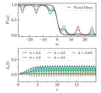
Figure 4: Upper panel: nonequilibrium distribution functions for a resonant electric field with $\varOmega=U=10$ and a series of amplitudes $A$. The dotted line is the Fermi–Dirac distribution at the bath temperature $\beta=1$. Lower panel: particle current in the lattice. For $A=3.831$ a net flow within the lattice and a nonequilibrium distribution remain clearly visible, such that the system cannot be in an effective equilibrium state.

The counterintuitive nature of a dissipation-free NESS might lead one to conclude that the system may be at an effective equilibrium state when driven at Bessel zero amplitudes. Interestingly, this is not the case. To show this, we plot the period averaged nonequilibrium distribution function $\bar{F}\left(\omega\right)=-\frac{i}{2}\frac{\bar{G}^{<}\left(\omega\right)}{\Im\bar{G}^{R}\left(\omega\right)}$ at $l=1$ in the top panel of Fig. 4. In equilibrium $\bar{F}(\omega)$ matches the Fermi–Dirac distribution $f\left(\omega\right)$ at the bath temperature. Driving the system modulates $\bar{F}(\omega)$ such that resonances / antiresonances appear at $\omega=-\frac{U}{2}\pm n\varOmega$ with $n\in\mathcal{N}$, corresponding to $n$-photon absorption processes. At an amplitude matching the first Bessel zero single-photon absorption is suppressed, but the spectrum retains a clear nonequilibrium shape. The lower panel of Fig. 4 shows the particle current $I_{n}(t)$ in the lattice at the same parameters. In equilibrium $I_{n}(t)$ vanishes within numerical uncertainty, as it must; but this happens at no other amplitude, including the Bessel zero case. We note that the time-averaged lattice current can be nonzero, but cancels with the lattice–bath current in agreement with particle conservation.

VI Conclusion

We considered an infinite-dimensional interacting many-body lattice model driven by periodic fields and coupled to a bath. For this model, we showed that it is possible to engineer a family of driven steady states with distinct nonequilibrium characteristics, but without time-averaged dissipation of energy between the system and bath. At the limit of high frequency driving we showed that this surprising result can be understood at the level of a simple analytical theory. Our numerical results are based on dynamical mean field theory, exact for this model; and on the noncrossing approximation at a physical regime where it is thought to be reliable. A variety of interesting questions can now be raised: since the noncrossing approximation can be lifted by a variety of modern numerical methods,(Cohen et al., 2015; Antipov et al., 2017; Dong et al., 2017; Profumo et al., 2015; Bertrand et al., 2019a, b; Moutenet et al., 2019) it will be of some interest to see whether this result survives an exact treatment. Another important challenge is to check whether the effect remains present for more realistic finite-dimensional models that may also feature nonlocal interactions, vibrational degrees of freedom and disorder. Finally, theoretical work will be needed to understand how generic this result is, and whether it can it be used to control dissipation and selectively engineer desired steady states in practical applications.