Blockage detection in networks: the area reconstruction method

Abstract.

In this note we present a reconstructive algorithm for solving the cross-sectional pipe area from boundary measurements in a tree network with one inaccessbile end. This is equivalent to reconstructing the first order perturbation to a wave equation on a quantum graph from boundary measurements at all network ends except one. The method presented here is based on a time reversal boundary control method originally presented by Sondhi and Gopinath for one dimensional problems and later by Oksanen to higher dimensional manifolds. The algorithm is local, so is applicable to complicated networks if we are interested only in a part isomorphic to a tree. Moreover the numerical implementation requires only one matrix inversion or least squares minimization per discretization point in the physical network. We present a theoretical solution existence proof, a step-by-step algorithm, and a numerical implementation applied to two numerical experiments.

1. Introduction

We present a reconstruction algorithm and its numerical implementation for solving for the pipe cross-sectional area in a water supply network from boundary measurements. Mathematically this is modelled by the frictionless waterhammer equations on a quantum graph, with Kirchhoff’s law and the law of continuity on junctions. The waterhammer equations on a segment $P={({0,\ell})}$ are given by [1, 2]

$$\partial_{t}H(t,x)=-\frac{a^{2}(x)}{gA(x)}\partial_{x}Q(t,x), t\in\mathbb{R},x\in P,$$ (1.1)

$$\partial_{t}Q(t,x)=-gA(x)\partial_{x}H(t,x), t\in\mathbb{R},x\in P,$$ (1.2)

where

• $H$ is the hydraulic pressure (piezometric head) inside the pipe $P$, with dimensions of length,

• $Q$ is the pipe discharge or flow rate in the direction of increasing $x$. Its dimension is length³/time,

• $a$ is the wave speed in length/time,

• $g$ is the graviational acceleration in length/time²,

• $A$ is the pipe’s internal cross-sectional area in length².

We model the network by a set of segments whose ends have been joined together. The segments model pipes. In this model we first fix a positive direction of flow on each pipe $P_{j}$, and set the coordinates ${({0,\ell_{j}})}$ on it. Then we impose Equations 1.1 and 1.2 on the segments. On the vertices, which model junctions, we require that $H(t,x)$ has a unique limit no matter which direction the point $x$ tends to the vertex. Moreover on any vertex $V$ we require that

$$\sum_{P_{j}\text{ connected to }V}\nu_{j}Q_{j}=0$$ (1.3)

where $\nu_{j}\in\{+1,-1\}$ gives the direction of the internal normal vector in coordinates $x$ to pipe $P_{j}$ at $V$, and $Q_{j}$ is the boundary flow of pipe $P_{j}$ at vertex $V$. In other words $\nu_{j}Q_{j}$ is the flow into the pipe $P_{j}$ at the vertex $V$. Hence the sum of the flows into the pipes at each vertex must be zero. Therefore there are no sinks or sources at the junctions, and also none in the network in general, except for the ones at the boundary of the network that are used to create our input flows for the measurements.

The inverse problem we are set to solve is the following one. We assume that the wave speed $a(x)=a$ is constant. If not, see Section 6. Given a tree network with $N+1$ ends $x_{0},x_{1},\ldots,x_{N}$, we can set the flow and measure the pressure on these points except for $x=x_{0}$. Using this information, can we deduce $A(x)$ for $x$ inside the network?

The problem of finding pipe areas arise in systems such as water supply networks and pressurized sewers, due to the formation of blockages during their lifetime [3, 4]. In water supply pipes, blockages increase energy consumption and increase the potential of water contamination. Blockages in sewer pipes increase the risk of overflows in waste-water collection systems and impose a risk to public health and environment. Detection of these anomalies improves the effectiveness of pipe replacement and maintenance, and hence improves environmental health.

An analogous and important problem is fault detection in electric cables and feed networks. This problem can be solved in the same way as blockage detection because of the analogy between waterhammer equations and Telegrapher’s equations [5].

Mathematically the simplest network is a segment joining $x_{1}$ to $x_{0}$. In this setting, the problem formulated as above was solved by [6]. Various other algorithms were developed for solving the one-segment problem both before and after. See [7] for a review. After a while some mathematicians started focusing on the network situation and others into higher dimensional manifolds. Others continued on tree networks, which are also the setting of this manuscript. For tree networks Belishev’s boundary control method [8, 9] showed that a tree network can be completely reconstructed after having access to all boundary points. These results were improved more recently by Avdonin and Kurasov [10]. A unified approach that uses Carleman estimates and is applicable to various equations on tree networks was introduced by Baudouin and Yamamoto [11]. Also, [12] implies that it is possible to solve the problem in the presence of various different boundary conditions when doing the measurements. A network having loops presents various challenges to solving for the cross-sectional area from boundary measurements [13]. In [10] the authors furthermore show that all but one boundary vertex is enough information, and also that if the network topology is known a-priori, then the simpler backscattering data is enough to solve the inverse problem. This latter data is easier to measure: the pressure needs to be measured only at the same network end from which the flow pulse is sent.

Our paper has two goals: 1) to solve the inverse problem by a reconstruction algorithm, and 2) to have a simple and concrete algorithm that is easy to implement on a computer. In other words we focus on the reconstruction aspect of the problem, given the full necessary data, and show that it is possible to build an efficient numerical algorithm for reconstruction. From the point of view of implementing the reconstruction, the papers cited above are of various levels of difficulty, and we admit that this is partly a question of experience and opinion. We view that apart from [6], all of them focus much on the important theoretical foundations, but lack in the clarity of algorithmic presentation for non-experts. Therefore one of the major points of this text is a clearly defined algorithm whose implementation does not require understanding its theoretical foundations. See Section 4.

Our method is based on the ideas of [6, 14] and is a continuation of our investigation of the single pipe case [3]. In both of them the main point is to use boundary control to produce a wave that would induce a constant pressure in a domain of influence at a certain given time. A simple integration by parts gives then the total volume covered by that domain of influence. Time reversal is the main tool which allows us to build that wave without knowing a-priori what is inside the pipe network.

A numerical implemetation and proof of a working regularization scheme for [14] in one space dimension was shown in [15]. Earlier, we studied [6] and tested it numerically in the context of blockage detection in water supply pipes [3] and also experimentally. We also showed that the method can be further extended to detect other types of faults such as leaks [16]. The one space-dimensional inversion algorithm can be implemented more simply than in [14, 15], even in the case of networks. This is the main contribution of this paper. Furthermore we provide a step-by-step numerical implementation and present numerical experiments. Our reconstruction algorithm is local and time-optimal. In other words if we are interested in only part of the network, we can do measurements on only part of the boundary. Furthermore the algorithm uses time-measurements just long enough to recover the part of interest. Intuitively, to reconstruct the area $A(x)$ at a location $x$, the wave must reach the location $x$ and reflects back to the measurement location. Any measurement done on a shorter time-interval will not be enough to recover it.

2. Governing Equations

Networks

Denote by $\mathbb{G}$ a tree network. Let $\mathbb{J}$ be the set of internal junction points and $\mathbb{P}$ the set of pipes, or segments. The boundary $\partial\mathbb{G}$ consists of all ends of pipes that are not junctions of two or more pipes. Each of them belongs to a single pipe unlike junction points which belong to three or more. There are no junction points that are connected to exactly two pipes: these two pipes are considered as one, and the point between is just an ordinary internal point.

Each pipe $P\in\mathbb{P}$ is modelled by a segment $({0,\ell})$ where $\ell$ is the length of the pipe. This defines a direction of positive flow on the pipe, namely from $x=0$ towards $x=\ell$. The pipes are connected to each other by junction points. Write $(x,P)\sim v$ if $v\in\mathbb{J}$, $x$ is the beginning ($x=0$) or endpoint ($x=\ell$) of pipe $P\in\mathbb{P}$, and the latter is connected to $v$ at the beginning ($x=0$) or end ($x=\ell$), respectively.

Example 2.1.

Figure 1. A simple network.

An example network is depicted in Figure 1. Here $\mathbb{J}=\{D\}$, $\partial\mathbb{G}=\{A,B,C\}$, $\mathbb{P}=\{AD,BD,DC\}$. Moreover here is a coordinate representation

$$AD=({0,$400\text{\,}\mathrm{m}$}) BD=({0,$300\text{\,}\mathrm{m}$}) DC=({0,$1000\text{\,}\mathrm{m}$})$$ , , ,

$$(0,AD)\sim A (0,BD)\sim B (0,DC)\sim D$$ , , ,

$$($400\text{\,}\mathrm{m}$,AD)\sim D ($300\text{\,}\mathrm{m}$,BD)\sim D ($1000\text{\,}\mathrm{m}$,DC)\sim C$$ , , .

Example 2.2.

Example 2.1 can be implemented numerically as follows. In total there are four vertices and three pipes. If vector indexing starts with $1$ we number points as $C=1$, $A=2$, $B=3$, $D=4$ and pipes as $AD=1$, $BD=2$, $DC=3$. The adjacency matrix Adj is defined so as pipe number i goes from vertex number Adj(i,1) to vertex number Adj(i,2).

⬇

V = 4; % number of vertices

L = [400; 300; 1000]; % length of pipes

Adj = [2 4; 3 4; 4 1]; % adjacency matrix

Equations

Inside pipe $P$ the perturbed pressure head $H$ and cross-sectional discharge $Q$ satisfy

$$\partial_{t}H(t,x)=-\frac{a^{2}}{gA(x)}\partial_{x}Q(t,x), t\in\mathbb{R},\quad x\in P,$$ (2.1)

$$\partial_{t}Q(t,x)=-gA(x)\partial_{x}H(t,x), t\in\mathbb{R},\quad x\in P,$$ (2.2)

where $a,A,g$ denote the wave speed, cross-sectional area and gravitational acceleration. The sign of $Q$ is chosen so that $Q>0$ means the flow goes from $0$ to $\ell$. In Example 2.1 the positive flow goes from $A$ to $D$, from $B$ to $D$ and from $D$ to $C$. The wave speed is assumed constant.

The pressure is a scalar: if $v\in\mathbb{J}$ connects two or more pipes $(x_{j},P_{j})\sim v$, $j=1,2,\ldots$, then $H$ has a unique value at $v$

$$\lim_{\begin{subarray}{c}x\to x_{j}\\ x\in P_{j}\end{subarray}}H(t,x)=\lim_{\begin{subarray}{c}x\to x_{k}\\ x\in P_{k}\end{subarray}}H(t,x),\qquad t\in\mathbb{R},\quad(x_{j},P_{j})\sim v\sim(x_{k},P_{k}).$$ (2.3)

The flow satisfies mass conservation, i.e. a condition analogous to Kirchhoff’s law. The total flow into a junction must be equal to the total flow out of the junction at any time. To state this as an equation we define the internal normal vector $\nu$ for any pipe end. If the pipe $P$ has coordinate representation ${(0,\ell)}$ then $\nu(0)=+1$ and $\nu(\ell)=-1$. Recall that $Q>0$ mean a positive flow from the direction of $0$ to $\ell$. This means that $\nu(x)Q(t,x)$ is the flow into the pipe at point $x\in\{0,\ell\}$. If it is positive then there is a net flow of water into $P$ through $x$. If it is negative then there is a net flow out of $P$ through $x$. Mass conservation is then written as

$$\sum_{(x,P)\sim v}\nu(x)Q(t,x)=0,\qquad t\in\mathbb{R},\quad v\in\mathbb{J}.$$ (2.4)

Initial conditions

The model assumes unperturbed initial conditions

$$H(t,x)=Q(t,x)=0,\qquad t<0,\quad x\in P$$ (2.5)

for any pipe $P\in\mathbb{P}$.

Direct problem

In this section we define the behaviour of the pressure $H$ and pipe cross-sectional discharge $Q$ in the network given a boundary flow and network structure. This is the direct problem. Recall that we have one inaccessible end of the network, $x_{0}$, whose boundary condition must be an inactive one, i.e. must not create waves when there are no incident waves. To make the problem mathematically well defined we choose for example Equation 2.7. Other options would work too, for example involving derivatives of $H$ or $Q$, but it is questionable how physically realistic such an arbitrary boundary condition is. The main point is that any inactive condition at the inaccessible end is allowed without risking the reconstruction. This is because the theoretical waves used in the calculations of our reconstruction algorithm never have to reach this final vertex, and so the boundary condition there never has a chance to modify reflected waves.

Definition 2.3.

We say that $H$ and $Q$ satisfy the network wave model with boundary flow $F:\mathbb{R}\times\partial\mathbb{G}\setminus\{x_{0}\}\to\mathbb{R}$ if $F(t,x)=0$ for $t<0$ and $H,Q$ satisfy Equations 2.1 and 2.2, the junction conditions of Equations 2.3 and 2.4 and the initial conditions of Equation 2.5. Furthermore $Q$ must satisfy the boundary conditions

$$\nu(x)Q(t,x)=F(t,x), \qquad x\in\partial\mathbb{G},x\neq x_{0},t\in\mathbb{R}$$ (2.6)

$$A(t)Q(t,x)+B(t)H(t,x)=0, \qquad x=x_{0},t\in\mathbb{R}$$ (2.7)

for some given functions or constants $A(t),B(t)$ that we do not need to know.

Remark.

Note that $\nu Q=F$ implies that $F$ is the flow into the network. If $F>0$ fluid enters, and if $F<0$ fluid is coming out.

Let us mention a few words about the unique solvability of the network wave model with a given boundary flow $F$. First of all we have not given any precise function spaces where the coefficients of the equation or the boundary flow would belong to. This means that it is not possible to find an exact reference for the solvability. On the other hand this is not a problem for linear hyperbolic problems in general.

The problem is a one-dimensional linear hyperbolic problem on various segments with co-joined boundary conditions. As the waves propagate locally in time and space, one can start with the solution to a wave equation on a single segment, as in e.g. Appendix 2 to Chapter V in [17]. Then when the wavefront approaches a junction, Equations 2.3 and 2.4 determine the transmitted and reflected waves to each segment joined there. Then the wave propagates again according to [17], and the boundary conditions are dealt with as in a one segment case. At no point is there any space to make any “choices”, and thus there is unique solvability. We will not comment on this further, but for more technical details we refer to [17] for the wave propagation in a segment and the boundary conditions, and to Section 3 of [8] for the wave propagation through junctions. For an efficient numerical algorithm to the direct problem, see [18].

Boundary measurements

The area reconstruction method presented in this paper requires the knowledge of the impulse-response matrix (IRM) for all boundary points except one, which we denote by $x_{0}$.

Definition 2.4.

We define the impulse-response matrix, or IRM, by $K=(K_{ij})_{i,j=1}^{N}$. For a given $i$ and $j$ we assume that $H$ and $Q$ satisfy the network wave model with boundary flow

$$\nu(x)Q(t,x)=\begin{cases}V_{0}\,\delta_{0}(t),&x=x_{i}\\ 0,&x\neq x_{i}\end{cases}$$ (2.8)

for $t\in\mathbb{R}$ and $x\in\partial\mathbb{G},x\neq x_{0}$. Here $V_{0}$ is the volume of fluid injected at $t=0$. Then we set

$$K_{ij}(t)=H(t,x_{j})/V_{0}$$ (2.9)

for any $t\in\mathbb{R}$.

The index $i$ represents the source and $j$ the receiver. Note also that the IRM gives complete boundary measurement information: if $\nu(x)Q(t,x_{i})=F(t,x_{i})$ were another set of injected flows at the boundary, then the corresponding boundary pressure would be given by

$$H(t,x_{j})=\sum_{\begin{subarray}{c}x_{i}\in\partial\mathbb{G}\\ x_{i}\neq x_{0}\end{subarray}}\int K_{ij}(t-s,x_{i})F(s,x_{i})ds$$ (2.10)

by the principle of superposition.

3. Area reconstruction algorithm

Strategy

Once the impulse-response matrix from Equation 2.9 has been measured, we have everything needed to determine the cross-sectional area in a tree network. As in the one pipe case [3], we will calculate special “virtual” boundary conditions, which if applied to the pipe system, would make the pressure constant in a given region at a given time. Exploiting this and the knowledge of the total volume of water added to the network by these virtual boundary conditions gives the total volume of the region. Slightly perturbing the given region reveals the cross-sectional area.

Multiply Equation 2.1 by $gA/a^{2}$ and integrate over a time-interval ${({0,\tau})}$, for a fixed $\tau>0$, and the whole network $\mathbb{G}$. This gives

$$\sum_{x_{j}\in\partial\mathbb{G}}\int_{0}^{\tau}\nu(x_{j})Q(t,x_{j})dt=\int_{\mathbb{G}}H(\tau,x)\frac{gA(x)}{a^{2}(x)}dx$$ (3.1)

if $H(0,x)=0$ and mass conservation from Equation 2.4 applies. Let $p\in\mathbb{G}$ be a point at which we would like to recover the cross-sectional area. To it we associate a set $D_{p}\subset\mathbb{G}$ which we shall define precisely later. Let us assume that there are boundary flows $Q_{p}(t,x_{j})$ so that at time $t=\tau$ we have

$$H(\tau,x)=\begin{cases}h_{0},&x\in D_{p},\\ 0,&x\notin D_{p},\end{cases}$$ (3.2)

for some fixed pressure $h_{0}$. Then from Equation 3.1 we have

$$\sum_{x_{j}\in\partial\mathbb{G}}\int_{0}^{\tau}\nu(x_{j})Q_{p}(t,x_{j})dt=\frac{h_{0}g}{a^{2}}\int_{D_{p}}A(x)dx.$$

Denote the integral on the left by $V(D_{p})$. We can calculate its values once we know $Q_{p}$, hence we know the value of the integral on the right. By varying the shape of $D_{p}$ we can then find the area $A(p)$.

Admissible sets

The only requirement for $D_{p}$ in the previous section was that Equation 3.2 holds. Boundary control, e.g. as in [9], implies that there are suitable boundary flows $Q_{p}$ such that the equation holds for any reasonable set $D_{p}$. However it is not easy to calculate the flows given an arbitrary $D_{p}$. In this section we define a class of such sets for which it is very simple to calculate the flows.

Let $p\in\mathbb{G}\setminus\mathbb{J}$ be a non-junction point in the network at which we wish to solve for the cross-section area $A(p)$. Since we have a tree network the point $p$ splits $\mathbb{G}$ into two networks. Let $D_{p}$ be the part that is not connected to the inaccessible boundary point $x_{0}$. The boundary of $D_{p}$ consists of let us say $y_{1},y_{2},\ldots,y_{k}$ and $p$, where the points $y_{j}$ are also boundary points of the original network.

For each boundary point $y_{j}\in\partial D_{p}$, $y_{j}\neq p$ define the action time

$$f(y_{j})=\operatorname{TT}(y_{j},p)$$ (3.3)

where $\operatorname{TT}$ gives the travel-time of waves from $y_{j}$ to $p$ calculated along the shortest path in $D_{p}$. Then set $f(x_{j})=0$ for $x_{j}\in\partial\mathbb{G}\setminus\partial D_{p}$.

Definition 3.1.

We say that $D_{p}$ is an admissible set associated with $p\in\mathbb{G}\setminus\mathbb{J}$ and with action time $f$, if $D_{p}$ and $f$ are defined as above given $p$.

It turns out that with the choice of admissible sets made above we have

$$D_{p}=\{x\in\mathbb{G}\mid\operatorname{TT}(x_{j},x)<f(x_{j})\text{ for some }x_{j}\in\partial\mathbb{G}\}.$$ (3.4)

This is because $D_{p}$ lies between $p$ and the boundary points $x_{j}$ at which $f(x_{j})\neq 0$. This gives a geometric interpretation to the set $D_{p}$, i.e. that it is the domain of influence of the action times $f(x_{j})$, $x_{j}\in\partial\mathbb{G}$. If we would have zero boundary flows at first, and then active boundary flows when $x_{j}\in\partial\mathbb{G}$, $\tau-f(x_{j})<t\leq\tau$, then the transient wave produced would have propagated throught the whole set $D_{p}$ at time $t=\tau$ but not at all into $\mathbb{G}\setminus D_{p}$.

Reconstruction formula for the area

Now that the form of the admissible sets have been fixed, we are ready to prove in detail what was introduced at the beginning of this section, namely a formula for solving the unknown pipe cross-sectional area. For simplicity we assume that the wave speed is constant.

Theorem 3.2.

Let $p\in\mathbb{G}\setminus\mathbb{J}$ be a non-junction point and $D_{p}$, $f$ the associated admissible set and action time. Let $\tau>\max f$. For a small time-interval $\Delta_{t}>0$ set

$$(f+\Delta_{t})(x_{j})=\begin{cases}f(x_{j})+\Delta_{t},&x_{j}\in\partial D_{p}\setminus\{p\},\\ 0,&x_{j}\in\partial\mathbb{G}\setminus\partial D_{p}.\end{cases}$$

For $\phi=f$ or $\phi=f+\Delta_{t}$ denote

$$D^{\phi}=\{x\in\mathbb{G}\mid\operatorname{TT}(x,x_{j})<\phi(x_{j})\text{ for some }x_{j}\in\partial D_{p}\setminus\{p\}\}$$ (3.5)

so $D^{f}=D_{p}$ and $D^{f+\Delta_{t}}$ is a slight expansion of the former.

Assume that $H_{\phi},Q_{\phi}$ satisfy the network wave model with a boundary flow $F$ which is nonzero only during the action time $\phi$, namely $F(t,x_{j})=0$ when $x_{j}\in\partial\mathbb{G}$, $x_{j}\neq x_{0}$ and $0\leq t\leq\tau-\phi(x_{j})$. Finally, assume that

$$H_{\phi}(\tau,x)=\begin{cases}h_{0},&x\in D^{\phi},\\ 0,&x\notin D^{\phi},\end{cases}$$ (3.6)

for some given pressure head $h_{0}>0$ at time $t=\tau$.

Denote by

$$V(\phi,\tau)=\frac{a^{2}}{h_{0}g}\sum_{x_{j}\in\partial D_{p}\setminus\{p\}}\nu(x_{j})\int_{0}^{\tau}Q_{\phi}(t,x_{j})dt$$

the total volume of fluid injected into the network from the boundary in the time-interval ${({0,\tau})}$ to create the waves $H_{\phi},Q_{\phi}$. Then

$$A(p)=\lim_{\Delta_{t}\to 0}\frac{V(f+\Delta_{t},\tau)-V(f,\tau)}{a\Delta_{t}}$$ (3.7)

gives the cross-sectional area of the pipe at $p$.

Proof.

The assumption about the boundary flow implies that

$$H_{\phi}(t,x_{j})=Q_{\phi}(t,x_{j})=0$$ (3.8)

in the same space-time set, i.e. when $x_{j}\in\partial\mathbb{G}$, $x_{j}\neq x_{0}$ and $0\leq t\leq\tau-\phi(x_{j})$. Consider Equation 2.1 for $H_{\phi},Q_{\phi}$ where $\phi=f$ or $\phi=f+\Delta_{t}$ is fixed. Multiply the equation by $gA/a^{2}$ and integrate $\int_{0}^{\tau}\int_{\mathbb{G}}\ldots dxdt$. This gives

$$-\int_{0}^{\tau}\int_{\mathbb{G}}\partial_{x}Q_{\phi}(t,x)dxdt=\int_{0}^{\tau}\int_{\mathbb{G}}\frac{gA(x)}{a^{2}}\partial_{t}H_{\phi}(t,x)dxdt.$$

The right-hand side is equal to

$$\frac{g}{a^{2}}\int_{\mathbb{G}}A(x)\big{(}H_{\phi}(\tau,x)-H_{\phi}(0,x)\big{)}dx=\frac{gh_{0}}{a^{2}}\int_{D^{\phi}}A(x)dx$$

because $H_{\phi}(0,x)=0$ by Equation 2.5. We will use the junction conditions of Equation 2.4 to deal with the left-hand side. But before that let us use a fixed coordinate system of the network $\mathbb{G}$.

Let the pipes of the network be $P_{1},\ldots,P_{n}$ and model them in coordinates by the segments ${({0,\ell_{1}})},\ldots,{({0,\ell_{n}})}$, respectively. On pipe $P_{k}$, denote by $H_{\phi,k}$ the scalar pressure head, and by $Q_{\phi,k}$ the pipe discharge into the positive direction. Then

$$\int_{\mathbb{G}}\partial_{x}Q_{\phi}(t,x)dx=\sum_{k=1}^{n}\int_{0}^{\ell_{k}}\partial_{x}Q_{\phi,k}(t,x)dx=\sum_{k=1}^{n}\big{(}Q_{\phi,k}(t,\ell_{k})-Q_{\phi,k}(t,0)\big{)}.$$

Note that $Q_{\phi,k}(t,\ell_{k})$ is simply the discharge out of the pipe $P_{k}$ at the latter’s endpoint represented by $x=\ell_{k}$ at time $t$. Similarly $-Q_{\phi,k}(t,0)$ is the discharge out from the other endpoint, the one represented by $x=0$. Now Equation 2.4 implies after a few considerations that

$$-\int_{\mathbb{G}}\partial_{x}Q_{\phi}(t,x)dx=\sum_{x_{j}\in\partial D_{p}\setminus\{p\}}\nu(x_{j})Q_{\phi}(t,x_{j}).$$

Namely, previously we saw that the integral is equal to the sum of the total discharge out of every single pipe. But the discharge out of one pipe must go into another pipe at junctions (there are no internal sinks or sources). Hence the discharges at the junctions cancel out, and only the ones at the boundary $\partial\mathbb{G}$ remain. The boundary values are zero on $\partial\mathbb{G}\setminus(\partial D_{p}\cup\{x_{0}\})$ by the definition of $f$ and $f+\Delta_{t}$. We also have zero initial values and a non-active boundary condition at $x_{0}$, hence $Q_{\phi}(t,x_{0})=0$ too. Thus we have shown that

$$\int_{D^{\phi}}A(x)dx=\frac{a^{2}}{gh_{0}}\sum_{x_{j}\in\partial D_{p}\setminus\{p\}}\nu(x_{j})Q_{\phi}(t,x_{j})=V(\phi,\tau).$$ (3.9)

Next, we will show that

$$V(f+\Delta_{t},\tau)-V(f,\tau)=\int_{D^{f+\Delta_{t}}\setminus D^{f}}A(x)dx.$$ (3.10)

Recall that $p$ is not a vertex. Hence it is on a unique pipe, let’s say ${({0,\ell})}$ and $p$ is represented by $x_{p}$ on this segment. Furthermore assume that (or change coordinates so that) the point represented by $0$ is in $D_{p}$, and the one by $\ell$ is not. This implies that the difference of sets $D^{f+\Delta_{t}}\setminus D^{f}$ is just a small segment on ${({0,\ell})}$.

Let us look at the effect of $\Delta_{t}$ on $D^{f+\Delta_{t}}$ which is defined in Equation 3.5. We have $x\in D^{f+\Delta_{t}}\setminus D^{f}$ if and only if $\operatorname{TT}(x,x_{j})<f(x_{j})+\Delta_{t}$ for some boundary point $x_{j}\in\partial D_{p}$, $x_{j}\neq p$, but also $\operatorname{TT}(x,x_{k})\geq f(x_{k})$ for all boundary points $x_{k}\in\partial D_{p}$, $x_{k}\neq p$. The former implies that $x$ is at most travel-time $\Delta_{t}$ from $D_{p}$, and the latter says that it should not be in $D_{p}$. In other words $D^{f+\Delta_{t}}\setminus D^{f}=\{x\in{({0,\ell})}\mid x_{p}\leq x<x_{p}+a\Delta_{t}\}$ and so

$$V(f+\Delta_{t},\tau)-V(f,\tau)=\int_{x_{p}}^{x_{p}+a\Delta_{t}}A(x)dx,$$ (3.11)

where we abuse notation and denote the cross-sectional area of the pipe modelled by ${({0,\ell})}$ at the location $x$ also by $A(x)$ without emphasizing that it is the area on this particular model of this particula pipe.

Equation 3.11 gives the area at $p$, $A(x_{p})$, by differentiating. Let $B(s)=\int_{x_{p}}^{x_{p}+s}A(x)dx$. Then $A(x_{p})=\partial_{s}B(0)$ and the right-hand side of Equation 3.11 is equal to $B(a\Delta_{t})$. The chain rule for differentiation gives

$$A(x_{p})=\partial_{s}B(s)_{|s=0}=\frac{1}{a}\partial_{\Delta_{t}}(B(a\Delta_{t}))_{|\Delta_{t}=0}=\frac{1}{a}\lim_{\Delta_{t}\to 0}\frac{V(f+\Delta_{t},\tau)-V(f,\tau)}{\Delta_{t}}$$

from which the claim follows. ∎

Solving for the area

In this section we will show one way in which boundary values of $Q$ can be determined so that the assumptions of Theorem 3.2 are satisfied. It is previously known that there are boundary flows giving Equation 3.2, for example by [9] where the authors show the exact $L^{2}$-controllability of the network both locally and in a time-optimal way. However there was no simple way of calculating such boundary flows and the numerical reconstruction algorithm of that paper does not seem computationally efficient as it uses a Gram–Schmidt orthogonalization process on a number of vectors inversely proportional to the network’s discretization size. We show that if the flow satisfies a certain boundary integral equation then this is the right kind of flow. Moreover, in the appendix we give a proof scheme for showing that the equation has a solution.

More recently various layer-peeling type of methods have appeard [10, 12]. The method we present here is based on another idea, one whose roots are in the physics of waves, namely time reversibility. This is in essence a combination of the one pipe case originally considered in [6], and of a fundamentally similar idea for higher dimensional manifolds introduced in [14]. In the latter the author considers domains of influence and action times on the boundary, and builds a boundary integral equation whose solution then reveals the unknown inside the manifold. This will be our guide.

Let us recall the unique continuation principle used for the area reconstruction method for one pipe in [3, 6]. Consider a pipe of length $\ell>0$, modelled by the interval ${({0,\ell})}$. Let $\mathcal{H}$ and $\mathcal{Q}$ satisfy the Waterhammer Equations 2.1 and 2.2 without requiring any initial conditions. Then

Lemma 3.3.

If $\mathcal{H}(t,0)=2h_{0}$ and $\mathcal{Q}(t,0)=0$ for $t_{m}<t<t_{M}$, then inside the pipe we would have $\mathcal{H}(t,x)=2h_{0}$ and $\mathcal{Q}(t,x)=0$ in the space-time triangle $x/a+\left\lvert t-(t_{M}+t_{m})/2\right\rvert<(t_{M}-t_{m})/2$, $0<x<\ell$. See Figure 2.

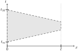
Figure 2. The region $\frac{x}{a}+\left\lvert t-\frac{t_{M}+t_{m}}{2}\right\rvert<\frac{t_{M}-t_{m}}{2}$, $0<x<\ell$.

The lemma was then used to build a virtual solution $H,Q$ satisfying also the initial conditions, and which would have $H(\tau,x)=h_{0}$ for $x<a\tau$ and $H(\tau,x)=0$ for $x>a\tau$ for a given $\tau>0$. Without going into detailed proofs, the same unique continuation idea works for a tree network. The reason is that one can propagate $\mathcal{H}=2h_{0}$, $\mathcal{Q}=0$ from one end of a pipe to the other, but by keeping in mind that the time-interval where these hold shrinks as one goes further into the pipe. Do this first on all the pipes that touch the boundary. Then use the junction conditions from Equations 2.3 and 2.4 to see that $\mathcal{H}=2h_{0}$, $\mathcal{Q}=0$ on the next junctions. Then repeat inductively. We have shown

Proposition 3.4.

Let $p\in\mathbb{G}\setminus\mathbb{J}$ and let $D_{p}\subset\mathbb{G}$ be admissible associated with $p$ and with action time $f$. Let $\mathcal{H},\mathcal{Q}$ satisfy Equations 2.1 and 2.2 and the junction conditions of Equations 2.3 and 2.4. Let $\tau\geq\max f$ and assume that

$$\mathcal{H}(t,x_{j})=2h_{0},\qquad\mathcal{Q}(t,x_{j})=0,\qquad x_{j}\in\partial\mathbb{G},\quad\left\lvert t-\tau\right\rvert<f(x_{j}).$$ (3.12)

Then $\mathcal{H}(t,x)=2h_{0}$ and $\mathcal{Q}(t,x)=0$ whenever $x\in\mathbb{G}$, $0<t<2\tau$ and

$$\operatorname{TT}(x,x_{j})+\left\lvert\tau-t\right\rvert<f(x_{j})$$ (3.13)

for some $x_{j}\in\partial\mathbb{G}$.

We can now write an integral equation whose solution gives waves with $H(\tau,x)=h_{0}$ for $x\in D_{p}$ and $H(\tau,x)=0$ for $x\notin D_{p}$ at time $t=\tau$.

Theorem 3.5.

Let $K_{ij}$ be the impulse-response matrix from Equation 2.9. If $A$ is constant near each network boundary point we have

$$K_{ij}(t)=\frac{a}{A(x_{i})g}\delta_{0}(t)\delta_{ij}+k_{ij}(t)$$

for some function $k_{ij}=k_{ji}$ that vanishes near $t=0$.

Let $p\in\mathbb{G}\setminus\mathbb{J}$ be and let $D_{p}\subset\mathbb{G}$ be the admissible set associated with $p$, and with action time $f$. Take $\tau\geq\max f$ and let $Q_{p}(t,x_{j})$ satisfy

$$h_{0} =\frac{a}{A(x_{j})g}\nu(x_{j})Q_{p}(t,x_{j})$$

$$\quad+\sum_{\begin{subarray}{c}x_{i}\in\partial\mathbb{G}\\ x_{i}\neq x_{0}\end{subarray}}\frac{\nu(x_{i})}{2}\int_{0}^{\tau}Q_{p}(s,x_{i})\big{(}k_{ij}(\left\lvert t-s\right\rvert)+k_{ij}(2\tau-t-s)\big{)}ds$$ (3.14)

when $x_{j}\in\partial\mathbb{G}$, $x_{j}\neq x_{0}$, $\tau-f(x_{j})<t\leq\tau$ and

$$Q_{p}(t,x_{j})=0$$ (3.15)

when $x_{j}\in\partial\mathbb{G}$, $x_{j}\neq x_{0}$ and $0\leq t\leq\tau-f(x_{j})$.

Then if $H,Q$ satisfy the network wave model with boundary flow $\nu Q_{p}$ we have

$$H(\tau,x)=\begin{cases}h_{0},&x\in D_{p},\\ 0,&x\in\mathbb{G}\setminus D_{p}.\end{cases}$$ (3.16)

Remark 3.6.

If one sets $Q_{p}(2\tau-t,x_{j})=Q_{p}(t,x_{j})$, one could instead have

$$h_{0}=\frac{a}{A(x_{j})g}\nu(x_{j})Q_{p}(t,x_{j})+\sum_{\begin{subarray}{c}x_{i}\in\partial\mathbb{G}\\ x_{i}\neq x_{0}\end{subarray}}\frac{\nu(x_{i})}{2}\int_{0}^{2\tau}Q_{p}(s,x_{i})k_{ij}(\left\lvert t-s\right\rvert)ds$$

with $x_{j}\in\partial\mathbb{G}$, $\left\lvert t-\tau\right\rvert<f(x_{j})$ and $Q_{p}(t,x_{j})=0$ for $\left\lvert t-\tau\right\rvert\geq f(x_{j})$.

Proof.

The claim for the impulse response matrix is standard. See for example Appendix 2 to Chapter V in [17] for the solution to the one segment setting, and then use mathematical induction and the junction conditions of Equations 2.3 and 2.4.

Extend $Q_{p}$ symmetrically past $\tau$, i.e. $Q_{p}(2\tau-t,x_{j})=Q_{p}(t,x_{j})$ for $0\leq t\leq\tau$ and $x_{j}\in\partial\mathbb{G}$, $x_{j}\neq x_{0}$. Continue $H$ and $Q$ to $0<t<2\tau$ while still having $Q=Q_{p}$ as the boundary condition at $x\neq x_{0}$, and Equation 2.7 when $x=x_{0}$. Define

$$\mathcal{H}(t,x)=H(t,x)+H(2\tau-t,x),\qquad\mathcal{Q}(t,x)=Q(t,x)-Q(2\tau-t,x)$$

for $x\in\mathbb{G}$ and $0<t<2\tau$. The symmetry of $Q_{p}$ implies that $\mathcal{Q}(t,x_{j})=0$ for $x_{j}\in\partial\mathbb{G}$, $x_{j}\neq x_{0}$ and $0<t<2\tau$.

For the pressure, recall that the properties of the impulse response matrix from Equation 2.10 imply that

$$H(t,x_{j})=\sum_{\begin{subarray}{c}x_{i}\in\partial\mathbb{G}\\ x_{i}\neq x_{0}\end{subarray}}\int_{-\infty}^{\infty}K_{ij}(t-s)\nu(x_{i})Q_{p}(s,x_{i})ds$$

for $x_{j}\in\partial\mathbb{G}$, $x_{j}\neq x_{0}$ and $0<t<2\tau$. It is then easy to calculate that

$$H(t,x_{j})=\frac{a}{A(x_{j})g}\nu(x_{j})Q_{p}(t,x_{j})+\sum_{\begin{subarray}{c}x_{i}\in\partial\mathbb{G}\\ x_{i}\neq x_{0}\end{subarray}}\int_{0}^{t}k_{ij}(t-s)\nu(x_{i})Q_{p}(s,x_{i})ds$$

because $K_{ij}(t-s)=0$ when $s>t$ and $Q_{p}(s,x_{i})=0$ when $s<0$. For $H(2\tau-t,x_{j})$ split the integral to get

$$\int_{0}^{2\tau-t}k_{ij}(2\tau-t-s)Q_{p}(s,x_{i})ds$$

$$\qquad=\int_{0}^{\tau}k_{ij}(2\tau-t-s)Q_{p}(s,x_{i})ds+\int_{\tau}^{2\tau-t}k_{ij}(2\tau-t-s)Q_{p}(s,x_{i})ds$$

$$\qquad=\int_{0}^{\tau}k_{ij}(2\tau-t-s)Q_{p}(s,x_{i})ds+\int_{t}^{\tau}k_{ij}(s-t)Q_{p}(s,x_{i})ds$$

where we again used the time-symmetry of $Q_{p}$. Summing all terms and using $Q_{p}(2\tau-t,x_{j})=Q_{p}(t,x_{j})$ we see that

$$\mathcal{H}(t,x_{j})=H(t,x_{j})+H(2\tau-t,x_{j})=2\frac{a}{A(x_{j})g}\nu(x_{j})Q_{p}(t,x_{j})$$

$$\quad+\sum_{\begin{subarray}{c}x_{i}\in\partial\mathbb{G}\\ x_{i}\neq x_{0}\end{subarray}}\nu(x_{i})\int_{0}^{\tau}Q_{p}(s,x_{i})\big{(}k_{ij}(\left\lvert t-s\right\rvert)+k_{ij}(2\tau-t-s)\big{)}ds=2h_{0}$$

when $x_{j}\in\partial\mathbb{G}$ and $\left\lvert t-\tau\right\rvert<f(x_{j})$. The assumptions of Proposition 3.4 are now satisfied and so $\mathcal{H}(t,x)=2h_{0}$ and $\mathcal{Q}(t,x)=0$ when $0<t<2\tau$ and $\operatorname{TT}(x,x_{j})+\left\lvert\tau-t\right\rvert<f(x_{j})$ for some $x_{j}\in\partial\mathbb{G}$. Equation 3.4 and the finite speed of wave propagation imply Equation 3.16. ∎

Remark 3.7.

Assuming an impulse-response matrix that is measured to infinite precision and without modelling errors, one can show that Equations 3.14 and 3.15 have a solution. The idea of the proof is shown in the appendix. The solution is not necessarily unique, but it gives a unique reconstructed cross-sectional area.

4. Step-by-step algorithm

Measuring the impulse-response matrix

Recall Equation 2.9: the impulse-response matrix $K=(K_{ij})_{i,j=1}^{N}$ is defined by $K_{ij}(t)=H(t,x_{j})/V_{0}$ where $H,Q$ solve the Waterhammer Equations 2.1 and 2.2, junction Equations 2.3 and 2.4, zero initial conditions of Equation 2.5 and a flow impulse of volume $V_{0}$ at the boundary vertex $x_{i}$ and zero flow at other accessible vertices, as in Equation 2.8. Here $x_{i},x_{j}$ with $i,j\neq 0$ are the accessible boundary points, and $x_{0}$ is the inaccessible one that doesn’t produce surges.

Solving for the cross-sectional area

In this second part of the step-by-step reconstruction algorithm we assume that the impulse-response matrix $K$ has been calculated. It can be either measured by closing all accessible ends, or by measuring the system response in a different setting (i.e. different boundary conditions), then pre-process the measured signal to obtain the desired matrix $K$.

Once the impulse-response matrix has been measured as discussed in the previous paragraph, the following mathematical algorithm can be applied to recover the cross-sectional area inside a chosen pipe or pipe-segment in the network.

Algorithm 1.

This algorithm calculates the cross-sectional area using a discretization and Algorithm 2.

1. Define $k_{ij}(t)$ for $i,j\neq 0$ by

   $$k_{ij}(t)=K_{ij}(t)-\frac{a}{A(x_{i})g}\delta_{0}(t)\delta_{ij}$$

   where $\delta_{ij}$ is the Kronecker delta.

2. Choose a point $p_{1}$ in the network that is not a junction. The algorithm will reconstruct the cross-sectional area starting from $p_{1}$ and going towards $x_{0}$ until it hits the endpoint $p_{2}$ of the current pipe.

3. Split the interval between $p_{1}$ and $p_{2}$ into pieces of length $\Delta_{x}$.

4. Let $p$ be any point between two pieces above that has not been chosen yet. Calculate the internal volume $V(p)$ using Algorithm 2.

5. Redo Item 4 for all the points in the discretization of the interval between $p_{1}$ and $p_{2}$, and save the values of $V(p)$ associated with the point $p$.

6. Denote the discretization by $(p(0)=p_{1},p(1),\ldots,p(M)\approx p_{2})$. Then the area at $p(k)$ is approximately the volume between the points $p(k)$ and $p(k+1)$ divided by $\Delta_{x}$. In other words

   $$A\big{(}p(k)\big{)}\approx\frac{V\big{(}p(k+1)\big{)}-V\big{(}p(k)\big{)}}{\Delta_{x}}.$$

   This would be an equality if $\Delta_{x}$ were infinitesimal, or if $A(p(k))$ would signify the average area over the interval $(p(k),p(k+1))$.

Algorithm 2.

This algorithm calculates the internal volume of the piece of network cut off by $p$: namely all points from which you have to pass through $p$ to get to $x_{0}$.

1. For any boundary point $x_{j}\neq x_{0}$ set

   $$f(x_{j})=\begin{cases}\operatorname{TT}(x_{j},p),&\text{if $p$ is between $x_{j}$ and $x_{0}$},\\ 0,&\text{if not},\end{cases}$$

   where $\operatorname{TT}$ gives the travel-time between points. It is just the distance in the network divided by the wave speed.

2. Take $\tau\geq\max f$ and fix a pressure head $h_{0}>0$.

3. For any boundary point $x_{j}\neq x_{0}$ and time $\tau-f(x_{j})<t\leq\tau$, using regularization if necessary, let $Q_{p}$ solve

   $$h_{0}=\frac{a}{A(x_{j})g}\nu(x_{j})Q_{p}(t,x_{j})$$ (4.1)

   $$+\sum_{\begin{subarray}{c}x_{i}\in\partial\mathbb{G}\\ x_{i}\neq x_{0}\end{subarray}}\frac{\nu(x_{i})}{2}\int_{0}^{\tau}Q_{p}(s,x_{i})\big{(}k_{ij}(\left\lvert t-s\right\rvert)+k_{ij}(2\tau-t-s)\big{)}ds$$

   and also simultanously set

   $$Q_{p}(t,x_{i})=0$$

   for boundary points $x_{i}\neq x_{0}$ and time $0\leq t\leq\tau-f(x_{j})$. Thus the integral above can be calculated on $\tau-f(x_{j})<s\leq\tau$.

4. Set

   $$V(p)=\frac{a^{2}}{h_{0}g}\sum_{x_{j}\in\partial\mathbb{G}}\int_{0}^{\tau}\nu(x_{j})Q_{p}(t,x_{j})dt.$$ (4.2)

   It is the internal volume of the pipe network that is on the other side of $p$ than the inaccessible end $x_{0}$.

5. Numerical experiments

All the programming here was done in GNU Octave [19].

Experiment 1 (Simple network with exact IRM).

We will start by solving for the trivial area of Example 2.1. Consider this a test for the implementation of the area reconstruction algorithm. We start by calculating the impulse-response matrix of vertices $A$ and $B$ while $C$ is inaccessible. $D$ is the junction.

Set $A(x)=$1\text{\,}{\mathrm{m}}^{2}$$ everywhere, the gravitational acceleration $g=$9.81\text{\,}\mathrm{m}\text{\,}{\mathrm{s}}^{-2}$$ and a wave speed of $a=$1000\text{\,}\mathrm{m}\text{\,}{\mathrm{s}}^{-1}$$.

⬇

%% Physical parameters

maxc = 1000; % maximal wave speed in the network

g = 9.81; % standard gravity value (m/s^2)

%% Network a-priori information

V = 4; % total number of vertices

L = [400; 300; 1000]; % L(j) length of pipe j

Adj = [1 4; 2 4; 4 3]; % pipe j goes from vertex Adj(j,1) to vertex Adj(j,2)

A0 = [1,1]; % area at accessible pipe ends

a0 = [maxc, maxc]; % wave speed at accessible pipe ends

Let us calculate the IRM by hand. If a flow of $V_{0}\delta_{0}(t)$ is induced at point $A$, then it creates a propagating solution $Q=V_{0}\delta(ax-t)$, $H=aV_{0}\delta(ax-t)/(gA)$ along $AD$. If a pressure pulse of magnitude $M\delta_{0}$ is incident to $D$, then it transmits two pulses of magnitude $2M\delta_{0}/3$ to $BD$ and $DC$, and reflects one pulse of magnitude $-M\delta_{0}/3$ back to $AD$. These follow from the junction conditions of Equations 2.3 and 2.4. Also, if a similar pressure pulse is incident to a boundary point with boundary condition $Q=0$, then a pulse of the same magnitude (no sign change) is reflected. However at that boundary point the pressure is measured as $2M\delta_{0}$. These considerations produce the following impulse-response matrix

$$K_{AA}(t) =\frac{a}{gA}\Big{(}\delta_{0}\big{(}t\big{)}-\frac{2}{3}\delta_{0}\big{(}t-$0.8\text{\,}\mathrm{s}$\big{)}+\frac{8}{9}\delta_{0}\big{(}t-$1.4\text{\,}\mathrm{s}$\big{)}+\frac{2}{9}\delta_{0}\big{(}t-$1.6\text{\,}\mathrm{s}$\big{)}+\ldots\Big{)}$$

$$K_{BB}(t) =\frac{a}{gA}\Big{(}\delta_{0}\big{(}t\big{)}-\frac{2}{3}\delta_{0}\big{(}t-$0.6\text{\,}\mathrm{s}$\big{)}+\frac{2}{9}\delta_{0}\big{(}t-$1.2\text{\,}\mathrm{s}$\big{)}+\frac{8}{9}\delta_{0}\big{(}t-$1.4\text{\,}\mathrm{s}$\big{)}+\ldots\Big{)}$$

$$K_{AB}(t) =\frac{a}{gA}\Big{(}\frac{4}{3}\delta_{0}\big{(}t-$0.7\text{\,}\mathrm{s}$\big{)}-\frac{4}{9}\delta_{0}\big{(}t-$1.3\text{\,}\mathrm{s}$\big{)}-\frac{4}{9}\delta_{0}\big{(}t-$1.5\text{\,}\mathrm{s}$\big{)}+\ldots\Big{)}$$

$$K_{BA}(t) =K_{AB}(t)$$

for time $0\leq t\leq$1.6\text{\,}\mathrm{s}$$.

We must have $2\tau\leq$1.6\text{\,}\mathrm{s}$$, and so the algorithm can solve for the area up to points of the network that are at most $a\tau=$800\text{\,}\mathrm{m}$$ from each accessible end. Hence we can solve for the area only up to $400\text{\,}\mathrm{m}$ in pipe $DC$ from the junction $D$. The reflections $k_{ij}$ used in Algorithm 1 are

$$k_{AA}(t) =\frac{a}{gA}\Big{(}-\frac{2}{3}\delta_{0}\big{(}t-$0.8\text{\,}\mathrm{s}$\big{)}+\frac{8}{9}\delta_{0}\big{(}t-$1.4\text{\,}\mathrm{s}$\big{)}+\frac{2}{9}\delta_{0}\big{(}t-$1.6\text{\,}\mathrm{s}$\big{)}+\ldots\Big{)}$$

$$k_{BB}(t) =\frac{a}{gA}\Big{(}-\frac{2}{3}\delta_{0}\big{(}t-$0.6\text{\,}\mathrm{s}$\big{)}+\frac{2}{9}\delta_{0}\big{(}t-$1.2\text{\,}\mathrm{s}$\big{)}+\frac{8}{9}\delta_{0}\big{(}t-$1.4\text{\,}\mathrm{s}$\big{)}+\ldots\Big{)}$$

$$k_{AB}(t) =\frac{a}{gA}\Big{(}\frac{4}{3}\delta_{0}\big{(}t-$0.7\text{\,}\mathrm{s}$\big{)}-\frac{4}{9}\delta_{0}\big{(}t-$1.3\text{\,}\mathrm{s}$\big{)}-\frac{4}{9}\delta_{0}\big{(}t-$1.5\text{\,}\mathrm{s}$\big{)}+\ldots\Big{)}$$

$$k_{BA}(t) =k_{AB}(t).$$

⬇

%% Measurements

dt = 10/maxc; % in one time-step the wave propagates 10m

experiment_duration = 1.61; % impulse-response matrix should go from time t=0 to experiment_duration.

t = (0:dt:experiment_duration)’;

k = cell(2,2); % k is the response matrix

% The below is calculated by hand for a network as above.

k{1,1} = a0(1)/(A0(1)*g) *(…

-2/3*1/dt.*(t >= 0.8-dt/2).*(t < 0.8+dt/2) …

+8/9*1/dt.*(t >= 1.4-dt/2).*(t < 1.4+dt/2) …

+2/9*1/dt.*(t >= 1.6-dt/2).*(t < 1.6+dt/2) …

);

k{2,2} = a0(2)/(A0(2)*g) *(…

-2/3*1/dt.*(t >= 0.6-dt/2).*(t < 0.6+dt/2)…

+2/9*1/dt.*(t >= 1.2-dt/2).*(t < 1.2+dt/2) …

+8/9*1/dt.*(t >= 1.4-dt/2).*(t < 1.4+dt/2) …

);

k{1,2} = a0(2)/(A0(2)*g) *(…

+4/3*1/dt.*(t >= 0.7-dt/2).*(t < 0.7+dt/2)…

-4/9*1/dt.*(t >= 1.3-dt/2).*(t < 1.3+dt/2) …

-4/9*1/dt.*(t >= 1.5-dt/2).*(t < 1.5+dt/2) …

);

k{2,1} = k{1,2};

Let us define the action time functions for various points $p$ in the network. If $p\in AD$ then the action time is

$$f^{AD}_{p}(x)=\begin{cases}TT(A,p),&x=A\\ 0,&x=B\\ 0,&x=C\end{cases}$$

and for $p\in BD$

$$f^{BD}_{p}(x)=\begin{cases}0,&x=A\\ TT(B,p),&x=B\\ 0,&x=C\end{cases}.$$

The travel-time from $A$ to $D$ is $0.4\text{\,}\mathrm{s}$, and from $B$ to $D$ it is $0.3\text{\,}\mathrm{s}$. Recall that the IRM has been measured only for time $t\leq$1.6\text{\,}\mathrm{s}$$. Hence we can solve for the area up to $400\text{\,}\mathrm{m}$ into pipe $DC$. Let the point $p\in DC$ be given by the action time function

$$f^{DC}_{p}(x)=\begin{cases}$0.4\text{\,}\mathrm{s}$+t_{p},&x=A\\ $0.3\text{\,}\mathrm{s}$+t_{p},&x=B\\ 0,&x=C\end{cases}$$

where $0\leq t_{p}\leq$400\text{\,}\mathrm{m}$/a=$0.4\text{\,}\mathrm{s}$$ is the travel-time from $D$ to $p$ and recalling that we can solve the area only up to $400\text{\,}\mathrm{m}$ from $D$.

⬇

%% Set parameters

tau = 0.8; % area will be solved up to 2*tau*maxc from accessible point furthest to inaccessible point x3.

assert(2*tau <= experiment_duration, ’Can recover area only up to experiment_duration*maxc/2.’);

reguparam = 1e-5; % Tikhonov regularization parameter

dx = dt*maxc; % into how big chunks we discretize the pipe

%% x-discretization

maxL = [L(1); L(2); tau*maxc - max(L(1),L(2))];

maxL = min(L,maxL); % maximum length of pipes that can be reached from all accessible vertices in time tau

M = floor(maxL/dx); % number of discretized segments of length dx in each pipe

%% Action times to various points in the network

f = cell(length(L),1); % a different action time formula for points on each pipe

% action times to pipe 1 (AD) points

f{1} = nan(M(1),2);

f{1}(:,1) = (1:M(1))’*dx./maxc;

f{1}(:,2) = zeros(size((1:M(1))’));

% action times to pipe 2 (BD) points

f{2} = nan(M(2),2);

f{2}(:,1) = zeros(size((1:M(2))’));

f{2}(:,2) = (1:M(2))’*dx./maxc;

% action times to pipe 3 (DC) points

f{3} = nan(M(3),2);

f{3}(:,1) = (L(1)+(1:M(3))’*dx)./maxc;

f{3}(:,2) = (L(2)+(1:M(3))’*dx)./maxc;

Let us apply Algorithm 1 next. The numerical implementation of Algorithm 2, makeHeq1, is in the appendix.

⬇

%% Solve for the cross-sectional area

% Initialize cells for saving various vectors

pipeVolume = cell(length(L),1); % volume of network cut by p

pipeArea = cell(length(L),1); % cross-sectional area at p

pipeX = cell(length(L),1); % x-coordinates of points p

for P=1:length(L) % P indexes the pipe number (AD, BD, DC)

assert(max(max(f{P})) - tau <= dt/4, ’Travel-times must be at most tau.’);

V = nan(M(P),1); % volume of the network up to points p

for p=1:M(P) % p indexes the point $p$ inside pipe P

% use Algorithm 2:

Qtau = makeHeq1(t, k, tau, f{P}(p,:), a0, g, A0, reguparam);

V(p) = 0;

% add to V the volume of water from each accessible end that would have gone INTO the pipe to make H=1 at t=tau:

for ii = 1:length(Qtau)

V(p) = sum(Qtau{ii})*dt + V(p)

end

end

pipeVolume{P} = maxc^2/g*V;

pipeArea{P} = (pipeVolume{P}(2:end)-pipeVolume{P}(1:end-1))/dx;

pipeX{P} = (1:M(P)-1)’.*dx;

end

A plot of the cross-sectional areas is shown in Figure 3.

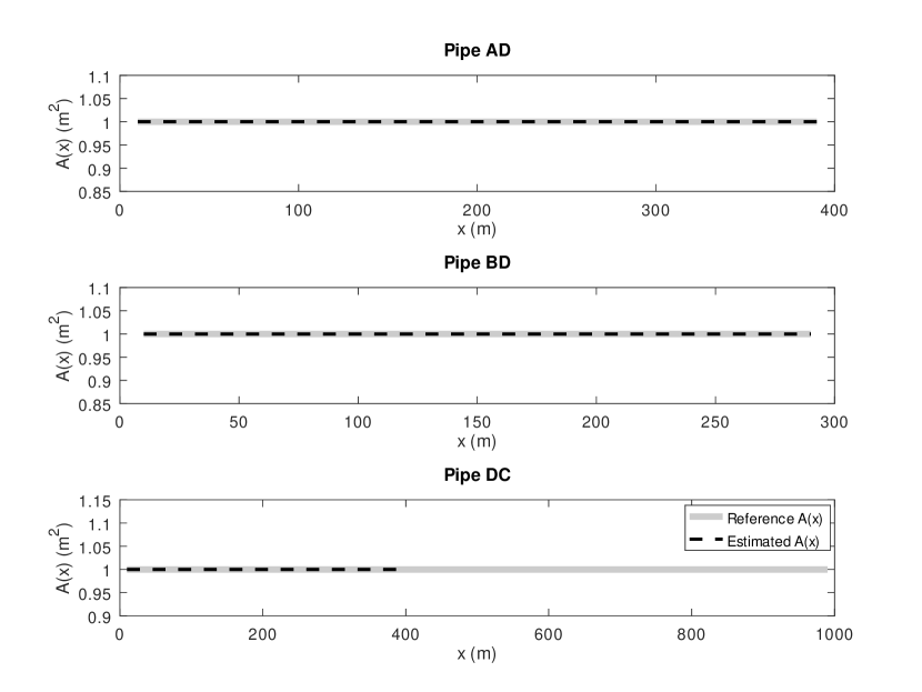
Figure 3. Solved cross-sectional areas of 1

Experiment 2 (Simulated IRM).

In the second experiment we consider a star-shaped network with four leaves, ending in points $A,B,C,D$. The internal node is denoted $E$. Let $D$ be the inaccessible end. Take the following lengths

$$AE=({0,$300\text{\,}\mathrm{m}$}) BE=({0,$400\text{\,}\mathrm{m}$}) CE=({0,$400\text{\,}\mathrm{m}$}) ED=({0,$500\text{\,}\mathrm{m}$}),$$ , , ,

as presented in Figure 4.

Figure 4. A more complicated network

We set a constant wave speed of $a=$1000\text{\,}\mathrm{m}\text{\,}{\mathrm{s}}^{-1}$$ everywhere and an area function that models blockages at certain locations.

⬇

%% physical parameters

maxc = 1000; % max wave speed

g = 9.81; % standard gravity value (m/s^2)

⬇

%% Network

V = 5; % total number of vertices

L = [300; 400; 400; 500]; % pipe lengths

Adj = [1 5; 2 5; 3 5; 5 4]; % to avoid display problems make arrows point towards inaccessible node (nbr 4)

Afunc1 = @(s)( ones(size(s)) );

Afunc2 = @(s)( 2*ones(size(s)) - (s>350).*(s<375).*0.6);

Afunc3 = @(s)( ones(size(s)) - (s>210).*(s<250).*0.2);

Afunc4 = @(s)( ones(size(s)) - (s>410).*(s<450).*0.4 - (s>150).*(s<250).*0.2);

afunc1 = @(s)( maxc*ones(size(s)) );

afunc2 = @(s)( maxc*ones(size(s)) );

afunc3 = @(s)( maxc*ones(size(s)) );

afunc4 = @(s)( maxc*ones(size(s)) );

Afunc = {Afunc1; Afunc2; Afunc3; Afunc4};

afunc = {afunc1; afunc2; afunc3; afunc4};

BVtype = [1; 1; 1; 1; NaN]; % Are inputs pressure (0) or flow (1)

We simulate the IRM by an a finite-difference time domain (FDTD) algorithm with the following caveats: we use a Courant number smaller than one, simulate using a high resolution, and then interpolate the IRM to a lower time-resolution and use this as input for the inversion algorithm. This is to avoid the inverse crime [20] which makes inversion algorithms give unrealistically good results when applied on data simulated with the same resolution or model as the inversion algorithm uses.

⬇

%% Measurements

% FDTD parameters

dx = 5;

courant = 0.95;

dt = courant*dx/maxc;

experiment_duration = 1.9;

doPlot = 0; % do we want to observe the FDTD simulation

% Boundary area and wave speed. Accessible ends are 1, 2 and 3

A0 = [Afunc1(0); Afunc2(0); Afunc3(0)];

a0 = [afunc1(0); afunc2(0); afunc3(0)];

For numerical reasons instead of sending a unit impulse $Q=\nu\delta$ we send a unit step-function, and then differentiate the measurements with respect to time. We will not show the implementation of FDTD and the self-explanatory functions removeInitialPulse, medianSmooth and differentiate because they are not the focus of this already rather long article. The main point is the inversion algorithm.

⬇

t = (0:dt:experiment_duration)’;

F = bndrySourceOn(t);

k = cell(3,3);

for ii=1:3

% Create input flows: constant flow at ii, otherwise zero

Vdata = cell(V,1);

for vv = 1:V

Vdata{vv} = zeros(size(F));

end

Vdata{ii} = F;

% Simulate the measurements with the given F

[Hhist, Qhist, thist] = FDTD(L, V, Adj, BVtype, Vdata, t, …

doPlot, maxc, g, dx, courant, Afunc, afunc);

% Remove the initial pulses and differentiate with respect to time

for jj=1:3

H = Hhist{jj};

if(ii==jj)

H = removeInitialPulse(H, thist, a0(ii), g, A0(ii));

end

% Smoothen slightly to make differentiation well behaved

H = medianSmooth(H, floor(0.02/(thist(2)-thist(1))));

H = differentiate(H, thist);

k{ii,jj} = H;

end

end

% Avoid the inverse crime by interpolation to a lower resolution

dx = 7;

dt = dx / maxc;

t = (thist(1): dt : experiment_duration)’;

for ii=1:size(k,1)

for jj=1:size(k,2)

k{ii,jj} = interp1(thist, k{ii,jj}, t);

end

end

The simulation gives us the following response matrix, as shown in Figure 5.

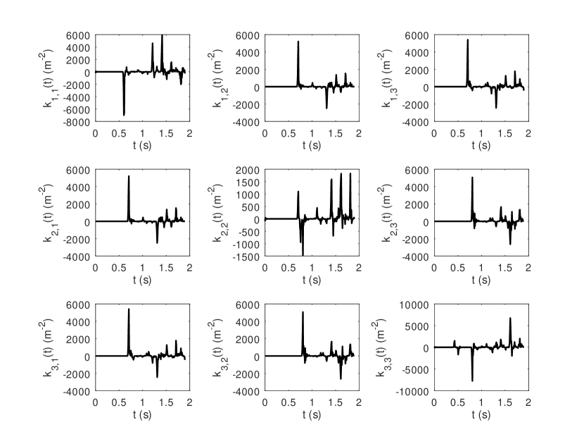
Figure 5. IRM for 2

Now solving the inverse problem has the same logic as in 1. There are two differences, a large one and a small one. The former is that the action time functions are of course different. This is what encodes the network topology for the inversion algorithm. And secondly we must use quite a lot of regularization when solving for the area of $ED$. This is because of the “numerical error” introduced on purpose by the Courant number smaller than one and interpolating the measurements to avoid doing an inverse cime.

⬇

%% Set parameters

reguparam = [1e-5, 1e-5, 1e-5, 1e0]; % regularization parameter to Tikhonov regularization in various pipes

tau = 0.9;

%% x-discretization

maxL = [L(1); L(2); L(3); tau*maxc - max([L(1) L(2) L(3)])];

maxL = min(L,maxL); % maximum length of pipes that can be reached from all accessible vertices in time tau

M = floor(maxL/dx); % Number of discretized segments of length dx in each pipe

f = cell(length(L),1);

%% Action times to various points in the network

% action times to pipe 1 (AE) points

f{1} = nan(M(1),3);

f{1}(:,1) = (1:M(1))’*dx./maxc;

f{1}(:,2) = zeros(size((1:M(1))’));

f{1}(:,3) = zeros(size((1:M(1))’));

% action times to pipe 2 (BE) points

f{2} = nan(M(2),3);

f{2}(:,1) = zeros(size((1:M(2))’));

f{2}(:,2) = (1:M(2))’*dx./maxc;

f{2}(:,3) = zeros(size((1:M(2))’));

% action times to pipe 3 (CE) points

f{3} = nan(M(3),3);

f{3}(:,1) = zeros(size((1:M(3))’));

f{3}(:,2) = zeros(size((1:M(3))’));

f{3}(:,3) = (1:M(3))’*dx./maxc;

% action times to pipe 4 (ED) points

f{4} = nan(M(4),3);

f{4}(:,1) = (L(1)+(1:M(4))’*dx)./maxc;

f{4}(:,2) = (L(2)+(1:M(4))’*dx)./maxc;

f{4}(:,3) = (L(3)+(1:M(4))’*dx)./maxc;

Then applying Algorithm 1 gives the solution as before.

⬇

%% Solve for the cross-sectional area

% Initialize cells for saving various vectors

pipeVolume = cell(length(L),1); % volume of network cut by p

pipeArea = cell(length(L),1); % cross-sectional area at p

pipeX = cell(length(L),1); % x-coordinate of points p

for P=1:length(L) % P indexes the pipe number (AE, BE, CE, ED)

assert(max(max(f{P})) - tau <= dt/4, ’Travel-times must be at most tau.’);

V = nan(M(P),1); % volume of the network up to points p

for p=1:M(P) % p indexes the point $p$ inside pipe P

Qtau = makeHeq1(t, k, tau, f{P}(p,:), a0,g,A0, reguparam(P));

V(p) = 0;

% add to V the total volume of water from accessible end that would have gone INTO the pipe to make H=1 at t=tau.

for ii = 1:length(Qtau)

V(p) = sum(Qtau{ii})*dt + V(p);

end

end

pipeVolume{P} = maxc^2/g*V;

pipeArea{P} = (pipeVolume{P}(2:end)-pipeVolume{P}(1:end-1))/dx;

pipeX{P} = (1:M(P)-1)’.*dx;

end

The solution is displayed in Figure 6. The gray uniform line represents the original cross-sectional area. The dashed line is the solution to the inverse problem.

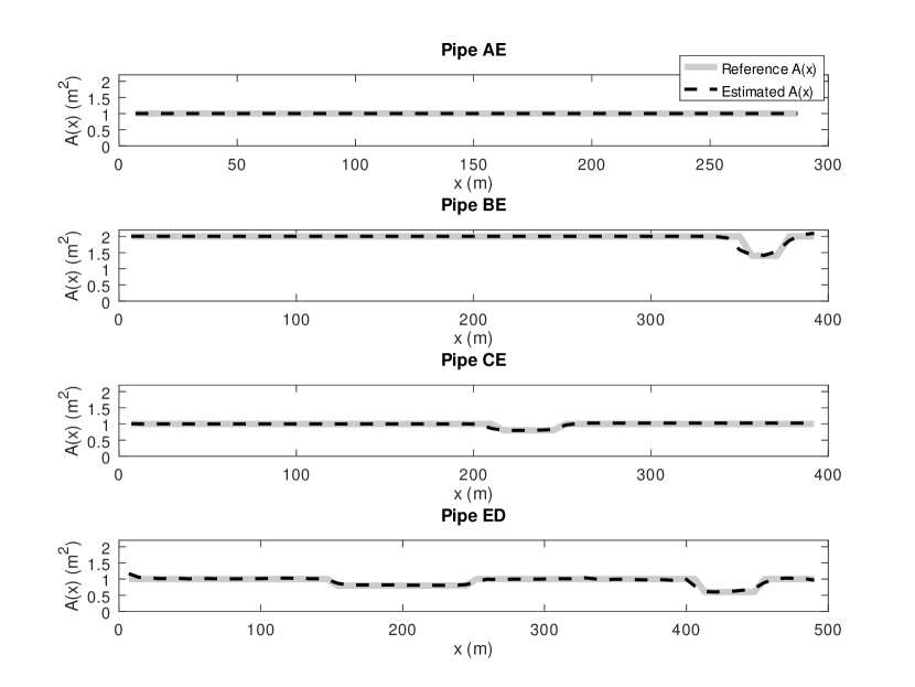
Figure 6. Solved cross-sectional areas of 2

6. Discussion and conclusions

We have developed and implemented an algorithm that reconstructs the internal cross-sectional area of pipes, filled with fluid, in a network arrangement. The region where the area is reconstructed must form a tree network and the input to our algorithm is the impulse-response measurements on all of the tree’s ends except for possibly one. The algorithm involves solving a boundary integral equation which is mathematically solvable in the case of perfect measurements and model (see the appendix). We wrote a step-by-step reconstruction algorithm and tested it using two numerical examples. The first one has a perfectly discretized measurement, and the second one has a discretization and numerical error introduced on purpose. Even with these errors, which are very typical when doing real-world measurements, Tikhonov regularization allows us to reconstruct the internal cross-sectional area with good precision. However this is just a first study of this algorithm, and a more in-depth investigation would be required for a more complete picture of its ability in the case of noise and other errors in the data. The theory is based on our earlier work [3] on solving for the area of one pipe, and on an iterative time-reversal boundary control algorithm [14] in the context of multidimensional manifolds.

We assumed in several places that the wave speed $a(x)$ is a known constant. What if it is not? We considered this situation for a single pipe in our previous article, [3]. In there, if the area is known and the speed is unknown, then the algorithm can be slightly modified to determine the wave speed profile along the pipe. If both the wave speed and the area are unknown then it can determine the hydraulic impedance $Z=a/gA$ as a function of the travel-time coordinate. However this is not so straightforward for the network case because of the more complicated geometry. What one should do first is find an algorithm to solve this problem: the wave speed is constant and known, the area is unknown, the topology of the network is known, but the pipe lengths are unknown. We leave this problem for future considerations as this article is already quite long. But it is an important question, because in fact in some applications the anomaly is the loss in pipe thickness rather than the change in pipe area and this is often revealed by finding the wave speed along the pipes assuming that the area remains unchanged [21].

In 1 we did not use regularization and the solution was perfect, as shown in Figure 3. However here we had the simplest tree network, the simplest area formula, and perfectly discretized measurements.

In 2 we simulated the measurements using a finite difference time domain (FDTD) method with Courant number smaller than one. Using Tikhonov regularization was essential, and produced the reconstruction shown in Figure 6. Without regularization one would get a large artifact, as in Figure 7.

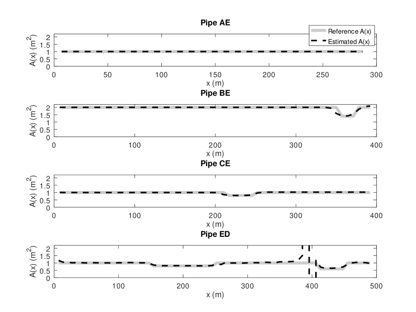
Figure 7. Solving without regularization

The reasons for using imperfect measurements are to demonstrate the algorithm’s stability. We could have calculated the impulse-response matrix using the more exact method of characteristics. However in reality, when dealing with data from actual measurement sensors, one would never get such perfect inputs to the inversion algorithm. First of all there are modelling errors, and secondly, measurement noise. By using FDTD with a small Courant number and also by inputting measurements with a rougher discretization than in the direct model we purposefully seek to avoid inverse crimes, as decribed in Section 1.2 of [20].

An inverse crime happens when the measurement data is simulated with the same model as the inversion algorithm assumes. Typically in these cases the numerical reconstruction looks unrealistically good, even with added measurement noise, and therefore does not reflect the method’s actual performance in real life, where models are always approximations.

Several directions of investigation still remain open. A more in-depth numerical study should be concluded, with proper statistical analysis and for example finding the signal to noise ratio that still gives meaningful reconstructions. There is also the issue of measuring the impulse-response matrix. It would be very much appreciated if there was no need to actually close almost all the valves in the network to perform measurements. Hence one could investigate various other types of boundary measurements and see how to process them to reveal the impulse-response matrix used here. To make even further savings in assessing the water supply network’s condition, one could also try implementing the theory from [10] as an algorithm. Their theoretical result only requires the so-called “backscattering data” from the network: instead of having to measure the full impulse-response matrix $(K_{ij})_{i,j=1}^{N}$ it would be enough to measure its diagonal $(K_{ii})_{i=1}^{N}$. This means that the pressure needs to be measured only at the same pipe end as the flow is injected. So the exact same type of measurement as is done for a single pipe, as in [3], should be done at each accessible network end. For a network with $N+1$ ends this translates into $N$ measurements compared to the $N^{2}$ for the full IRM.

Lastly we comment on our algorithm. What is interesting about it, is that there is no need to solve the area in the whole network at the same time. To save on computational costs one could for example reconstruct the cross-sectional area only in a small region of interest in a single pipe even when the network is otherwise quite large. Alternatively one could parallelize the process and solve for the whole network very fast using multiple computational cores. These would likely be impossible when having only the backscattering data described above.

The steps in Algorithms 1 and 2 describe the reconstruction process in detail. In essence only a single matrix inversion (or least squares or other minimization) is required for solving the area at any given point in the network. The size of this matrix depends on how finely the impulse-response matrix has been discretized, and how far from the boundary this point is. The rougher the discretization, the faster this step. However having a poor discretization leads to a larger numerical error, and one might then need to use a regularization scheme. All the numerical examples in this article were performed with an office laptop from 2008, and they took a few minutes to calculate including simulating the measurements. The algorithm is computationally light, simple to implement, and thus suitable for practical applications.

7. Acknowledgements

This research was partly funded by the fullowing grants.

• T21-602/15R Smart Urban water supply systems(Smart UWSS), and

• 16203417 Blockages in water pipes: theoretical and experimental study of wave-blockage interaction and detection.

Furthermore all authors declare that there are no conflicts of interest in this paper.

8. Appendix

8.1. Existence of a solution

We give a list of the steps involved in proving that the equation in Theorem 3.5 has a solution when the impulse-response matrix has been measured exactly and there is no modelling errors. Since the ultimate goal for our work is on assessing the quality of water supply network pipes, in the end there will be both modelling errors and measurement noise, so we will not give a complete formal proof. However we give enough details so that any mathematician specialized in the wave equation can fill the gaps after choosing suitable function space classes and assumptions for the various objects.

1. Given $p\in\mathbb{G}\setminus\mathbb{J}$ which defines the admissible set $D_{p}$ and action time $f$ according to Definition 3.1, and with $\tau>\max f$ and $h_{0}>0$, we want to solve

   $$h_{0} =\frac{a}{A(x_{j})}\nu(x_{j})Q_{p}(t,x_{j})$$

   $$\qquad+\sum_{x_{i}\in\partial\mathbb{G}\setminus\mathbb{J}}\frac{\nu(x_{i})}{2}\int_{0}^{\tau}Q_{p}(s,x_{i})\big{(}k_{ij}(\left\lvert t-s\right\rvert)+k_{ij}(2\tau-t-s)\big{)}ds$$

   when $\tau-f(x_{j})<t\leq\tau$, $x_{j}\in\partial\mathbb{G}\setminus\{x_{0}\}$, and $Q_{p}(s,x_{j})=0$ when $t\leq\tau-f(x_{j})$, $x_{j}\in\mathbb{G}\setminus\{x_{0}\}$.

2. We extend boundary data from the interval $(0,\tau)$ to $(-\infty,+\infty)$ and also absorb the interior boundary normal, by writing

   $$\mathscr{Q}_{p}(t,x_{j})=\begin{cases}\nu(x_{j})Q_{p}(t,x_{j}),&0\leq t\leq\tau,\\ \nu(x_{j})Q_{p}(2\tau-t,x_{j}),&\tau<t\leq 2\tau,\\ 0,&\text{otherwise}.\end{cases}$$

3. Solving

   $$\tilde{h}_{0}(t,x_{j}) =\frac{a}{A(x_{j})}\mathscr{Q}_{p}(t,x_{j})$$

   $$\qquad+\sum_{x_{i}\in\partial\mathbb{G}\setminus\mathbb{J}}\frac{\chi(t,x_{j})}{2}\int_{0}^{2\tau}\mathscr{Q}_{p}(s,x_{i})k_{ij}(\left\lvert t-s\right\rvert)ds$$

   in

   $$L^{2}_{0} =\Big{\{}F\in L^{2}(\mathbb{R}\times\partial\mathbb{G}\setminus\{x_{0}\})\,\Big{|}\,$$

   $$\qquad F(t,x_{j})=0\text{ if }\left\lvert t-\tau\right\rvert\geq f(x_{j}),\,F(2\tau-t,x_{j})=F(t,x_{j})\Big{\}}$$

   where

   $$\chi(t,x_{j})=\begin{cases}1,&\left\lvert t-\tau\right\rvert<f(x_{j}),\\ 0,&\left\lvert t-\tau\right\rvert\geq f(x_{j}),\end{cases}\qquad\tilde{h}_{0}(t,x_{j})=h_{0}\chi(t,x_{j})$$

   is equivalent to solving the equation of Item 1 in the corresponding $L^{2}$-based space. We equip $L^{2}_{0}$ with the inner product

   $$\langle A,B\rangle=\sum_{x_{j}\in\partial\mathbb{G}\setminus\mathbb{J}}\int_{0}^{2\tau}A(t,x_{j})\overline{B(t,x_{j})}dt$$

   where the complex conjugation can be ignored because all of our numbers are real.

4. The equation in Item 3 can be written as $\tilde{h}_{0}=\mathscr{K}\mathscr{Q}_{p}$ in $L^{2}_{0}$. Here we define the operator $\mathscr{K}$ by

   $$\mathscr{K}F(t,x_{j}) =\frac{a}{A(x_{j})}F(t,x_{j})$$

   $$\qquad+\sum_{x_{i}\in\partial\mathbb{G}\setminus\mathbb{J}}\frac{\chi(t,x_{j})}{2}\int_{0}^{2\tau}F(s,x_{i})k_{ij}(\left\lvert t-s\right\rvert)ds$$

   and it is a well-defined operator if $k_{ij}$ is a distribution of order $0$ which is the case if the cross-sectional area function $A$ is piecewise smooth for example. It indeed maps $L^{2}_{0}\to L^{2}_{0}$ satisfying the support and time-symmetry conditions.

5. We will show that $\mathscr{K}$ is a Fredholm operator $L^{2}_{0}\to L^{2}_{0}$ that is positive semidefinite.

6. Recall the travel-time function $TT$, the action time function $f$ and the admissible set $D_{p}$ from Item 1. Define

   $$\Omega =\Big{\{}(t,x)\in\mathbb{R}\times\mathbb{G}\,\Big{|}\,$$

   $$\qquad TT(x,x_{j})+\left\lvert t-\tau\right\rvert<f(x_{j})\text{ for some }x_{j}\in\partial\mathbb{G}\setminus\{x_{0}\}\Big{\}},$$

   $$t_{\pm}(x) =\tau\pm\max_{x_{j}\in\partial\mathbb{G}\setminus\{x_{0}\}}\big{(}f(x_{j})-TT(x,x_{j})\big{)}.$$

   The set $\Omega$ coincides with the set where unique continuation from the boundary holds, as in Proposition 3.4. One can show that

   $$\Omega=\{(t,x)\in\mathbb{R}\times\mathbb{G}\mid x\in D_{p},t_{-}(x)<t<t_{+}(x)\}.$$

7. Let $F\in L^{2}_{0}$ be given and fixed. Let $H,Q:\mathbb{R}\times\mathbb{G}\to\mathbb{R}$ satisfy the network wave model of Definition 2.3 with boundary flow $F$.

8. We see that $H(t,x)=Q(t,x)=0$ when $x\in D_{p}$ and $t\leq t_{-}(x)$. This follows from the zero initial conditions, finite speed of wave propagation and the definition of $t_{\pm}$ and the action time function $f$.

9. Define

   $$S=\frac{\sqrt{gA}}{a}H+\frac{\mu}{\sqrt{gA}}Q$$

   where $\mu(x)=+1$ if the positive direction of the coordinates at $x$ points towards $p$, and $\mu(x)=-1$ otherwise. Then one sees that

   $$\big{(}\partial_{x}-\tfrac{\mu}{a}\partial_{t}\big{)}(QH)=-\frac{1}{2}\partial_{t}(S^{2})$$

   in $t\in\mathbb{R}$, $x\in\mathbb{G}\setminus\mathbb{J}$.

10. By Items 6, 8 and 9 we see that

    $$-\frac{1}{2}\int_{\Omega}\partial_{t}(S^{2})dtdx =-\frac{1}{2}\int_{D_{p}}\big{(}S^{2}(t_{+}(x),x)-S^{2}(t_{-}(x),x)\big{)}dx$$

    $$=-\frac{1}{2}\int_{D_{p}}S^{2}(t_{+}(x),x)dx\leq 0.$$

11. By Items 9 and 10 and the divergence theorem we have

    $$0 \geq\int_{\Omega}\big{(}\partial_{x}-\tfrac{\mu}{a}\partial_{t}\big{)}(QH)dtdx=\int_{\Omega}\nabla_{t,x}\cdot\big{(}-\tfrac{\mu}{a}QH,QH\big{)}dtdx$$

    $$=\int_{\partial\Omega}\nu_{t,x}\cdot\big{(}-\tfrac{\mu}{a},1\big{)}QHd\sigma(t,x)$$

    where $\nu_{t,x}$ is the external unit normal vector to $\Omega$ at $(t,x)\in\partial\Omega$.

12. Let us split $\partial\Omega$ next. By Item 6 we see that

    $$\partial\Omega =\{(t,x_{j})\mid x_{j}\in\partial\mathbb{G}\setminus\{x_{0}\},\left\lvert t-\tau\right\rvert\leq f(x_{j})\}$$

    $$\qquad\cup\{(t,x)\mid x\in D_{p},t=t_{+}(x)\}\cup\{(t,x)\mid x\in D_{p},t=t_{-}(x)\}$$

    $$\qquad\cup\{(\tau,p)\}.$$

13. On the first set in Item 12 the external unit normal $\nu_{t,x_{j}}$ is given by $\nu_{t,x_{j}}=(0,-\nu(x_{j}))$ because $\nu$ was defined as the internal normal at the pipe ends.

14. Consider the second set in Item 12. On each individual pipe segment $P\subset D_{p}$ the map $x\mapsto t_{+}(x)$ is linear (affine). How does $t_{+}$ change when we go from $x$ to $x+\Delta x$? Recall that $\left\lvert\Delta x\right\rvert=a\left\lvert\Delta t\right\rvert$, and since $(t_{+}(x),x)$ follows the characteristics, so $t_{+}(x+\Delta x)=t_{+}(x)\pm\Delta x/a$. Its value decreases if $\Delta x>0$ and the positive direction of the coordinates $x$ point towards $p$. Both of these follow from Item 6 and the definition of the action time function $f$. By the definition of $\mu$ in Item 9 we see that

    $$\frac{\Delta x}{t_{+}(x+\Delta x)-t_{+}(x)}=-\frac{a}{\mu}.$$

    Thus the normal has a slope of $\mu/a$ and so

    $$\nu_{t,x}=\frac{(a,\mu)}{\sqrt{a^{2}+\mu^{2}}}=\frac{(a,\mu)}{\sqrt{1+a^{2}}}.$$

15. By Items 7, 8, 10, 11, 12, 13 and 14 we get

    $$0 \geq-\frac{1}{2}\int_{D_{p}}S^{2}(t_{+}(x),x)dx=\int_{\partial\Omega}\nu_{t,x}\cdot\big{(}-\tfrac{\mu}{a},1\big{)}QHd\sigma(t,x)$$

    $$=\sum_{x_{j}\in\partial\mathbb{G}\setminus\mathbb{J}}\int_{\tau-f(x_{j})}^{\tau+f(x_{j})}-F(t,x_{j})H(t,x_{j})dt$$

    $$\qquad+\int_{D_{p}}\frac{(a,\mu)}{\sqrt{1+a^{2}}}\cdot\big{(}-\tfrac{\mu}{a},1\big{)}(QH)(t_{+}(x),x)dx$$

    $$\qquad+\int_{D_{p}}\nu_{t,x}\cdot\big{(}-\tfrac{\mu}{a},1\big{)}(QH)(t_{-}(x),x)dx+0$$

    which gives

    $$\sum_{x_{j}\in\partial\mathbb{G}\setminus\mathbb{J}}\int_{0}^{2\tau}F(t,x_{j})H(t,x_{j})dt=\frac{1}{2}\int_{D_{p}}S^{2}(t_{+}(x),x)dx\geq 0$$

    by the support condition of $F\in L^{2}_{0}$ given in Item 3. In detail we see that the $D_{p}$-integrals vanish because of the following. Firstly we see that $(a,\mu)\cdot(-\mu/a,1)=0$ making the first integral over $D_{p}$ vanish. Secondly, by Item 8, $(QH)(t_{-}(x),x)=0$ for $x\in D_{p}$. The integral over the singleton $(t,s)=(\tau,p)$ is zero because $QH$ is a function since $F$ is too.

16. Recall Equation 2.10 and the splitting of the IRM $K$ into the impulse and response matrices in Theorem 3.5. Thus

    $$H(t,x_{j})=\frac{a}{A(x_{j})g}F(t,x_{j})+\sum_{x_{i}\in\partial\mathbb{G}\setminus\{x_{0}\}}\int_{0}^{t}F(s,x_{i})k_{ij}(t-s)ds.$$

17. Combining Items 15 and 16 and changing the order of integration in double integrals, we arrive at

    $$\langle\mathscr{K}F,F\rangle=\frac{1}{2}\int_{D_{p}}S^{2}(t_{+}(x),x)dx\geq 0$$

    for arbitrary $F\in L^{2}_{0}$ and where $S,H,Q$ are defined by Items 7 and 9.

18. We cannot show that $\mathscr{K}F=0$ implies $F=0$ unless the network is a single pipe. For a counter example choose a three-pipe network with constant unit area and wave speed, and each pipe is of unit length. Then send a pulse from one end and the same with opposite sign from another end. These pulses meet at the junction at the exact same time and cancel out the pressure there, so nothing propagates to the third pipe. Then they continue on the original two pipes until they hit the boundaries. The boundary flow $F$ should be then chosen so that these pulses are absorbed completely instead of reflecting back. This boundary flow $F$ gives $\langle\mathscr{K}F,F\rangle=0$ by Item 17, but $F\neq 0$.

19. The existence of a solution follows from the following: that $\mathscr{K}$ is self-adjoint and Fredholm, and that $\tilde{h}_{0}\perp\ker\mathscr{K}$, so then there is $F$ giving $\mathscr{K}F=\tilde{h}_{0}$. We shall show these next.

20. If we assume that $A(x)$ is smooth enough, then the components of the response matrix $(k_{ij})_{i,j=1}^{N}$ have at most a finite number of delta-functions arising from the junctions of $\mathbb{G}$ (in the time-interval ${({0,2\tau})}$), and are otherwise a function. Hence $\mathscr{K}$ can be split into a multiplication by nonvanishing functions, a finite number of translations that are also multiplied by such functions, and a smoothing integral operator which is compact $L^{2}_{0}\to L^{2}_{0}$. The identity and translations multiplied by non-vanishing functions are Fredholm operators, and the rest is compact. Hence the whole $\mathscr{K}$ is Fredholm. The space $L^{2}_{0}$ is Hilbert, and $\mathscr{K}$ is easily seen to be symmetric there because $k_{ij}=k_{ji}$. It is a bounded operator. Hence it is self-adjoint. Thus $\mathscr{K}$ is a self-adjoint Fredholm operator.

21. Let $w(s)=\int_{\mathbb{G}}H(s,x)\frac{gA}{a^{2}}dx$ where $H,Q$ are given by Item 7. By differentiating with respect to $s$, using Equation 2.1, calculating the $x$-integral, and integrating with respect to $s$ we see that

    $$\int_{D_{p}}H(\tau,x)\frac{gA}{a^{2}}dx=w(\tau)=\sum_{x_{j}\in\partial\mathbb{G}\setminus\{x_{0}\}}\int_{0}^{\tau}\nu(x_{j})Q(s,x_{j})ds$$

    because $Q=0$ near the boundary point $x_{0}$ up to time $\tau$. This is the same as in Equation 3.1.

22. Let $F\in L^{2}_{0}$ with $\mathscr{K}F=0$ and $H,Q$ as in Item 7. Set $h_{0}=0$ in Theorem 3.5 to conclude that $H(\tau,x)=0$ for $x\in\mathbb{G}$. Recall that the equations in that theorem are formulated using $\mathscr{K}$ here (see Item 3).

23. The time-symmetry of $F\in L^{2}_{0}$ gives the first equality below. Items 21 and 22 give the second and third equality, respectively. So

    $$\langle\tilde{h}_{0},F\rangle=\sum_{x_{j}\in\partial\mathbb{G}\setminus\{x_{0}\}}2h_{0}\int_{0}^{\tau}F(s,x_{j})ds=2h_{0}\int_{D_{p}}H(\tau,x)\frac{gA}{a^{2}}dx=0.$$

    Hence $\tilde{h}_{0}\perp\ker\mathscr{K}=\ker\mathscr{K}^{\ast}$, the latter because of self-adjointness, so

    $$\tilde{h}_{0}\in(\ker\mathscr{K}^{\ast})^{\perp}=\overline{\operatorname{ran}\mathscr{K}}=\operatorname{ran}\mathscr{K}$$

    because the range of a Fredholm operator is closed. In other words there is $F\in L^{2}_{0}$ such that $\mathscr{K}F=\tilde{h}_{0}$, and thus there is a solution to the equations in Theorem 3.5.

8.2. Numerical reconstruction algorithm

We describe here the numerical implementation of Algorithm 2. Its inputs include tHist, K, the discretized time-variable vector and cell containing the discretized components of the response matrix $k=(k_{ij})_{i,j=1}^{N}$ and f which is a vector modeling the discretized action time function. Other inputs are a0, A0, which are vectors containing the wave speed and cross-sectional area at the boundary points of the network, and tau, g, reguparam are scalars representing $\tau$, the constant of gravity $g$, and the Tikhonov regularization parameter used in the inversion of Equation 4.1. Its output, Qtau, is a cell whose components are discretizations of $t\mapsto Q_{p}(t,x_{j})$ that solved Equation 4.1 for the various boundary points $x_{j}$.

⬇

function Qtau = makeHeq1(tHist, K, tau, f, a0, g, A0, reguparam)

dt = tHist(2)-tHist(1);

nBndryPts = size(K,1);

We write first the $N$ (=nBndryPts) integral equations containing the $N$ response function components. This shall be indexed by j (pipe end where pressure measured) and i (pipe end where pulse sent from). Recall the equation,

$$h_{0}=\frac{a}{A(x_{j})g}q(t,x_{j})+\sum_{i=1}^{N}\frac{1}{2}\int_{0}^{\tau}q(t,x_{i})(k_{ij}(\left\lvert t-s\right\rvert)+k_{ij}(2\tau-t-s))ds$$

for $j=1,\ldots,N$ and $\tau-f(x_{j})<t\leq\tau$. But recall that we must still set $q(t,x_{j})=0$ when $t\leq\tau-f(x_{j})$. Our numerical implementation assumes that $h_{0}=1$.

We will write the equation above as H*q = RHS where $q$ is a block vector where each block is indexed by $i$ and

$$q^{i}=[q(dt,x_{i});q(2\,dt,x_{i});...;q(M\,dt,x_{i})]$$

with $M=\lfloor{\tau/dt}\rfloor$. Each component of RHS is either $h_{0}=1$ or $0$. We do a piecewise constant approximation of all of these functions and equations. We discretize t=l*dt, s=k*dt with l,k=1,...,M.

⬇

M = floor(tau/dt); % Number of time-steps of length dt in (0,tau).

% Discard unneeded measurements:

tHist = tHist(1:2*M);

for i = 1:nBndryPts

for j = 1:nBndryPts

K{i,j} = K{i,j}(1:2*M);

end

end

tVec = (1:M)*dt; lVec = 1:M;

sVec = (1:M)*dt; kVec = 1:M;

[t,s] = ndgrid(tVec,sVec);

[l,k] = ndgrid(lVec,kVec);

Set the tolerance for floating point numbers next. If two numbers are at most tolerance from each other, then they are considered the same. Without doing this, some numerical errors might happen when comparing two floating point numbers that are close to each other. This would cause errors of the order of $dx$ in the area reconstruction. We can now start discretizing the integral equation.

⬇

tol = dt/4;

Mij = nan(M,M); % Block (j,i) of matrix H

H = nan(nBndryPts*M, nBndryPts*M); % The linear operator

h0j = nan(M,1); % Block of RHS corresponding to j

RHS = nan(nBndryPts*M,1); % The RHS vector having 1’s or 0’s

for j = 1:nBndryPts

h0j = ones(M,1);

h0j((tVec - (tau - f(j)) <= tol)) = 0;

RHS( (j-1)*M + (1:M) ) = h0j;

for i = 1:nBndryPts

% Use 2*M-(l-1)-(k-1)=2*M+2-l-k for the time-reversal.

Mij = 0.5 * dt * ( K{i,j}(1+abs(l-k)) + K{i,j}(2*M+2-l-k) );

Recall that $q(s,x_{i})$ must be zero when $s\leq\tau-f(x_{i})$. Hence the columns of the matrix that hit the indices corresponding to $s\leq\tau-f(x_{i})$ should be zero. Similarly, when $t\leq\tau-f(x_{j})$ we want the equation to give $q(t,x_{j})=0$, so the part coming from the integral must be zeroed. Then add the “identity”-type part of the integral equation, and save the block into the final matrix.

⬇

Mij((s - (tau - f(i)) <= tol)) = 0;

Mij((t - (tau - f(j)) <= tol)) = 0;

if i==j

Mij = Mij + a0(j)/(A0(j)*g) .* eye(M);

end

H( (j-1)*M + (1:M), (i-1)*M + (1:M) ) = Mij;

end

end

Next, we solve the integral equation for $q$ using Tikhonov regularization. The simplest way would be to set
q = [H; sqrt(reguparam)*eye(size(H))] \ [RHS; zeros(size(RHS))];
but it is unnecessarily slow. For a faster solution we first remove all the rows and columns which would look like $0=0$. The vector nz shows the indices that are not forced to be zero, i.e. those where $\tau-f(x_{i})<s$. Then we remove the corresponding rows and columns from $H$. Then solve the equation.

⬇

nz = false(nBndryPts*M,1);

for i=1:nBndryPts

nz( (i-1)*M + (1:M) ) = ((sVec - (tau - f(i))) > tol);

end

H = H(nz, nz);

qnz = [H; sqrt(reguparam)*eye(size(H))] …

\ [RHS(nz); zeros(size(RHS(nz)))];

q = zeros(nBndryPts*M,1);

q(nz) = qnz;

Finally split the vector q into a cell whose components correspond to the boundary flows at the different boundary points.

⬇

Qtau = cell(nBndryPts, 1);

for i=1:nBndryPts

Qtau{i} = q( (i-1)*M + (1:M) );

end

end

References

- [1] Ghidaoui M S, Zhao M, McInnis D A, et al. (2005) A review of water hammer theory and practice. Applied Mechanics Reviews 58: 49–76. doi:10.1115/1.1828050.
- [2] Wylie E B, Streeter V L, Suo L (1993) Fluid transients in systems. 6th edition. Prentice Hall. ISBN 978-0-1332-2173-2.
- [3] Zouari F, Blåsten E, Louati M, et al. (2019) Internal pipe area reconstruction as a tool for blockage detection. Journal of Hydraulic Engineering 145: 04019019. doi:10.1061/(ASCE)HY.1943-7900.0001602.
- [4] Tolstoy A I (2010) Waveguide monitoring (such as sewer pipes or ocean zones) via matched field processing. The Journal of the Acoustical Society of America 128: 190–194. doi:10.1121/1.3436521.
- [5] Jing L, Wang W, Li Z, et al. (2018) Detecting impedance and shunt conductance faults in lossy transmission lines. IEEE Transactions on Antennas and Propagation .
- [6] Sondhi M M, Gopinath B (1971) Determination of vocal tract shape from impulse response at the lips. The Journal of the Acoustical Society of America 49: 1867–1873. doi:10.1121/1.1912593.
- [7] Bruckstein A M, Levy B C, Kailath T (1985) Differential methods in inverse scattering. SIAM Journal on Applied Mathematics 45: 312–335. doi:10.1137/0145017.
- [8] Belishev M I (2004) Boundary spectral inverse problem on a class of graphs (trees) by the BC method. Inverse Problems 20: 647–672. ISSN 0266-5611. doi:10.1088/0266-5611/20/3/002.
- [9] Belishev M I, Vakulenko A F (2006) Inverse problems on graphs: recovering the tree of strings by the BC-method. J Inverse Ill-Posed Probl 14: 29–46. ISSN 0928-0219. doi:10.1163/156939406776237474.
- [10] Avdonin S, Kurasov P (2008) Inverse problems for quantum trees. Inverse Probl Imaging 2: 1–21. ISSN 1930-8337. doi:10.3934/ipi.2008.2.1.
- [11] Baudouin L, Yamamoto M (2015) Inverse problem on a tree-shaped network: unified approach for uniqueness. Appl Anal 94: 2370–2395. ISSN 0003-6811. doi:10.1080/00036811.2014.985214.
- [12] Avdonin S A, Mikhaylov V S, Nurtazina K B (2015) On inverse dynamical and spectral problems for the wave and Schrödinger equations on finite trees. The leaf peeling method. Zap Nauchn Sem S-Peterburg Otdel Mat Inst Steklov (POMI) 438: 7–21. ISSN 0373-2703. doi:10.1007/s10958-017-3388-2.
- [13] Belishev M I, Wada N (2009) On revealing graph cycles via boundary measurements. Inverse Problems 25: 105011, 21. ISSN 0266-5611. doi:10.1088/0266-5611/25/10/105011.
- [14] Oksanen L (2011) Solving an inverse problem for the wave equation by using a minimization algorithm and time-reversed measurements. Inverse Probl Imaging 5: 731–744. ISSN 1930-8337. doi:10.3934/ipi.2011.5.731.
- [15] Korpela J, Lassas M, Oksanen L (2016) Regularization strategy for an inverse problem for a dimensional wave equation. Inverse Problems 32: 065001, 24. ISSN 0266-5611. doi:10.1088/0266-5611/32/6/065001.
- [16] Zouari F, Louati M, Blåsten E, et al. (2019) Multiple defects detection and characterization in pipes. In Proceedings of the 13th International Conference on Pressure Surges.
- [17] Courant R, Hilbert D (1962) Methods of mathematical physics. Vol. II: Partial differential equations. (Vol. II by R. Courant.). Interscience Publishers (a division of John Wiley & Sons), New York-London.
- [18] Karney B W, McInnis D (1992) Efficient calculation of transient flow in simple pipe networks. Journal of Hydraulic Engineering 118: 1014–1030. doi:10.1061/(ASCE)0733-9429(1992)118:7(1014).
- [19] Eaton J W, Bateman D, Hauberg S, et al. (2018) GNU Octave version 4.4.0 manual: a high-level interactive language for numerical computations. URL https://www.gnu.org/software/octave/doc/v4.4.1/.
- [20] Kaipio J, Somersalo E (2005) Statistical and computational inverse problems, volume 160 of Applied Mathematical Sciences. Springer-Verlag, New York. ISBN 0-387-22073-9.
- [21] Gong J, Lambert M F, Simpson A R, et al. (2014) Detection of localized deterioration distributed along single pipelines by reconstructive MOC analysis. Journal of Hydraulic Engineering 140: 190–198. doi:10.1061/(ASCE)HY.1943-7900.0000806.