Probing the anomalous triple gauge boson couplings in $e^{+}e^{-}\to W^{+}W^{-}$ using $W$ polarizations with polarized beams

Abstract

We study the anomalous $W^{+}W^{-}V$ ($V=\gamma,Z$) couplings in $e^{+}e^{-}\to W^{+}W^{-}$ using the complete set of polarization observables of $W$ boson with longitudinally polarized electron ($e^{-}$) and positron ($e^{+}$) beams. For the effective $W^{+}W^{-}V$ couplings, we use the most general Lorentz invariant form factor parametrization as well as $SU(2)\times U(1)$ invariant dimension-$6$ effective operators. We estimate simultaneous limits on the anomalous couplings using the Markov-Chain–Monte-Carlo (MCMC) method for an $e^{+}e^{-}$ collider running at center of mass energy of $\sqrt{s}=500$ GeV and the integrated luminosity of ${\cal L}=100$ fb^-1, $3.2$ ab^-1 and $4$ ab^-1. The best limits on the anomalous couplings are obtained for $e^{-}$ and $e^{+}$ polarization being $(\pm 0.8,\mp 0.6)$ for both $100$ fb^-1 and $3.2$ ab^-1 of luminosity.

I Introduction

The non-Abelian gauge symmetry $SU(2)\times U(1)$ of the Standard Model (SM) allows the $WWV$ ($V=\gamma,Z$) couplings after the electroweak symmetry breaking (EWSB) by the Higgs field discovered at the large hadron collider (LHC) Chatrchyan:2012xdj . To test the EWSB, the $WWV$ couplings have to be measured precisely, which is still lacking. We intend to study the measurement of these couplings using polarization observables of the spin-$1$ boson Bourrely:1980mr ; Abbiendi:2000ei ; Ots:2004hk ; Boudjema:2009fz ; Aguilar-Saavedra:2015yza ; Rahaman:2016pqj ; Nakamura:2017ihk . To test the SM $WWV$ couplings, one has to hypothesize beyond the SM (BSM) couplings and make sure they do not appear at all or are severely constrained. One approach is to consider $SU(2)\times U(1)$ invariant higher dimension effective operators which provide the $WWV$ form factors after EWSB Buchmuller:1985jz . The effective Lagrangian considering the higher dimension operators can be written as

$${\cal L}_{eft}={\cal L}_{SM}+\sum_{i}\frac{c_{i}^{{\cal O}(6)}}{\Lambda^{2}}{\cal O}_{i}^{(6)}+\sum_{i}\frac{c_{i}^{{\cal O}(8)}}{\Lambda^{4}}{\cal O}_{i}^{(8)}+\dots,$$ (1)

where $c_{i}^{{\cal O}(6,8)}$ are the couplings of the higher dimension operators ${\cal O}_{i}^{(6,8)}$ and $\Lambda$ is the energy scale below which the theory is valid. To the lowest order (up to dimension-$6$) the operators contributing to $WWV$ couplings are Hagiwara:1993ck ; Degrande:2012wf

$${\cal O}_{WWW} = \mbox{Tr}[W_{\mu\nu}W^{\nu\rho}W_{\rho}^{\mu}],$$

$${\cal O}_{W} = (D_{\mu}\Phi)^{\dagger}W^{\mu\nu}(D_{\nu}\Phi),$$

$${\cal O}_{B} = (D_{\mu}\Phi)^{\dagger}B^{\mu\nu}(D_{\nu}\Phi),$$

$${\cal O}_{\widetilde{WWW}} = \mbox{Tr}[\widetilde{W}_{\mu\nu}W^{\nu\rho}W_{\rho}^{\mu}],$$

$${\cal O}_{\widetilde{W}} = (D_{\mu}\Phi)^{\dagger}\widetilde{W}^{\mu\nu}(D_{\nu}\Phi),$$ (2)

where $\Phi$ is the Higgs doublet field and

$$D_{\mu} = \partial_{\mu}+\frac{i}{2}g\tau^{I}W^{I}_{\mu}+\frac{i}{2}g^{\prime}B_{\mu},$$

$$W_{\mu\nu} = \frac{i}{2}g\tau^{I}(\partial_{\mu}W^{I}_{\nu}-\partial_{\nu}W^{I}_{\mu}+g\epsilon_{IJK}W^{J}_{\mu}W^{K}_{\nu}),$$

$$B_{\mu\nu} = \frac{i}{2}g^{\prime}(\partial_{\mu}B_{\nu}-\partial_{\nu}B_{\mu}).$$ (3)

Here $g$ and $g^{\prime}$ are the $SU(2)$ and $U(1)$ couplings, respectively. Among these operators, ${\cal O}_{WWW}$, ${\cal O}_{W}$ and ${\cal O}_{B}$ are $CP$-even, while ${\cal O}_{\widetilde{WWW}}$ and ${\cal O}_{\widetilde{W}}$ are $CP$-odd. These effective operators, after EWSB, also provide $HZV$ and $HWW$ couplings, which can be examined in various processes, e.g., $ZV/ZW/HV/HW$ production processes. These processes may contain some other effective operators as well. We note that the $W$ pair production process also contains anomalous couplings other than the aTGC Zhang:2016zsp ; Baglio:2019uty . However, for simplicity, we study this process only with the anomalous gauge boson couplings.

The other alternative to step beyond the SM $WWV$ structure is to consider the most general Lorentz invariant effective form factors in a model independent way. A Lagrangian for the above parametrization is given by Hagiwara:1986vm

$${\cal L}_{WWV} = ig_{WWV}\left(g_{1}^{V}(W_{\mu\nu}^{+}W^{-\mu}-W^{+\mu}W_{\mu\nu}^{-})V^{\nu}\right.$$ (4)

$$+ ig_{4}^{V}W_{\mu}^{+}W^{-}_{\nu}(\partial^{\mu}V^{\nu}+\partial^{\nu}V^{\mu})$$

$$- ig_{5}^{V}\epsilon^{\mu\nu\rho\sigma}(W_{\mu}^{+}\partial_{\rho}W^{-}_{\nu}-\partial_{\rho}W_{\mu}^{+}W^{-}_{\nu})V_{\sigma}$$

$$+ \frac{\lambda^{V}}{m_{W}^{2}}W_{\mu}^{+\nu}W_{\nu}^{-\rho}V_{\rho}^{\mu}+\frac{\widetilde{\lambda^{V}}}{m_{W}^{2}}W_{\mu}^{+\nu}W_{\nu}^{-\rho}\widetilde{V}_{\rho}^{\mu}$$

$$+ \left.\kappa^{V}W_{\mu}^{+}W_{\nu}^{-}V^{\mu\nu}+\widetilde{\kappa^{V}}W_{\mu}^{+}W_{\nu}^{-}\widetilde{V}^{\mu\nu}\right).$$

Here $W_{\mu\nu}^{\pm}=\partial_{\mu}W_{\nu}^{\pm}-\partial_{\nu}W_{\mu}^{\pm}$, $V_{\mu\nu}=\partial_{\mu}V_{\nu}-\partial_{\nu}V_{\mu}$, $\widetilde{V}^{\mu\nu}=1/2\epsilon^{\mu\nu\rho\sigma}V_{\rho\sigma}$, and the overall coupling constants are defined as $g_{WW\gamma}=-g\sin\theta_{W}$ and $g_{WWZ}=-g\cos\theta_{W}$, with $\theta_{W}$ being the weak mixing angle. In the SM, $g_{1}^{V}=1$, $\kappa^{V}=1$ and other couplings are zero. The anomalous part in $g_{1}^{V}$, $\kappa^{V}$ would be $\Delta g_{1}^{V}=g_{1}^{V}-1$, $\Delta\kappa^{V}=\kappa^{V}-1$, respectively. The couplings $g_{1}^{V}$, $\kappa^{V}$ and $\lambda^{V}$ are $CP$-even (both $C$ and $P$-even), while $g_{4}^{V}$ (odd in $C$, even in $P$), $\widetilde{\kappa^{V}}$ and $\widetilde{\lambda^{V}}$ (even in $C$, odd in $P$) are $CP$-odd. On the other hand $g_{5}^{V}$ is both $C$ and $P$-odd making it $CP$-even. We label these sets of $14$ anomalous couplings to be $c_{i}^{\cal L}$ as given in Eq. (22) in appendix A for later uses.

On restricting to the $SU(2)\times U(1)$ gauge, the coupling ($c_{i}^{\cal L}$) of the Lagrangian in Eq. (4) can be written in terms of the couplings of the operators in Eq. (I) as Hagiwara:1986vm ; Hagiwara:1993ck ; Wudka:1994ny ; Degrande:2012wf

$$\Delta g_{1}^{Z} = c_{W}\frac{m_{Z}^{2}}{2\Lambda^{2}},$$

$$g_{4}^{V} = g_{5}^{V}=\Delta g_{1}^{\gamma}=0,$$

$$\lambda^{\gamma} = \lambda^{Z}=\lambda^{V}=c_{WWW}\frac{3g^{2}m_{W}^{2}}{2\Lambda^{2}},$$

$$\widetilde{\lambda^{\gamma}} = \widetilde{\lambda^{Z}}=\widetilde{\lambda^{V}}=c_{\widetilde{WWW}}\frac{3g^{2}m_{W}^{2}}{2\Lambda^{2}},$$

$$\Delta\kappa^{\gamma} = (c_{W}+c_{B})\frac{m_{W}^{2}}{2\Lambda^{2}},$$

$$\Delta\kappa^{Z} = (c_{W}-c_{B}\tan^{2}\theta_{W})\frac{m_{W}^{2}}{2\Lambda^{2}},$$

$$\widetilde{\kappa^{\gamma}} = c_{\widetilde{W}}\frac{m_{W}^{2}}{2\Lambda^{2}},$$

$$\widetilde{\kappa^{Z}} = -c_{\widetilde{W}}\tan^{2}\theta_{W}\frac{m_{W}^{2}}{2\Lambda^{2}}.$$ (5)

It is clear from above that some of the vertex factor couplings are dependent on each other and they are

$$\Delta g_{1}^{Z}=\Delta\kappa^{Z}+\tan^{2}\theta_{W}\Delta\kappa^{\gamma},$$

$$\widetilde{\kappa^{Z}}+\tan^{2}\theta_{W}\widetilde{\kappa^{\gamma}}=0.$$ (6)

We label the non-vanishing $9$ couplings in $SU(2)\times U(1)$ gauge as $c_{i}^{{\cal L}_{g}}$ given in Eq. (23) in appendix A for later uses.

The anomalous $WWV$ couplings have been studied in the effective operator approach as well as in the effective vertex formalism subjected to $SU(2)\times U(1)$ invariance for $e^{+}$-$e^{-}$ collider Gaemers:1978hg ; Hagiwara:1986vm ; Bilchak:1984ur ; Hagiwara:1992eh ; Choudhury:1996ni ; Choudhury:1999fz ; Wells:2015eba ; Buchalla:2013wpa ; Zhang:2016zsp ; Berthier:2016tkq ; Bian:2015zha ; Bian:2016umx , Large Hadron electron collider (LHeC)  Biswal:2014oaa ; Cakir:2014swa ; Li:2017kfk , $e$-$\gamma$ collider Kumar:2015lna and hadron collider (LHC) Baur:1987mt ; Dixon:1999di ; Bian:2015zha ; Falkowski:2016cxu ; Bian:2016umx ; Butter:2016cvz ; Azatov:2017kzw ; Baglio:2017bfe ; Li:2017esm ; Baglio:2018bkm ; Bhatia:2018ndx ; Chiesa:2018lcs ; Rahaman:2019lab ; Baglio:2019uty ; Azatov:2019xxn . Some $CP$-odd $WWV$ couplings have been studied in Refs. Choudhury:1999fz ; Li:2017esm ; Rahaman:2019lab .

On the experimental side, the anomalous $WWV$ couplings have been explored and stringent limits on them have been obtained at the LEP Abbiendi:2000ei ; Abbiendi:2003mk ; Abdallah:2008sf ; Schael:2013ita , the Tevatron Aaltonen:2007sd ; Abazov:2012ze , the LHC Khachatryan:2016poo ; Aad:2016ett ; Aad:2016wpd ; Chatrchyan:2013yaa ; RebelloTeles:2013kdy ; ATLAS:2012mec ; Chatrchyan:2012bd ; Aad:2013izg ; Chatrchyan:2013fya ; Aaboud:2017cgf ; Sirunyan:2017bey ; Aaboud:2017fye ; Sirunyan:2017jej ; Sirunyan:2019gkh ; Sirunyan:2019dyi ; Sirunyan:2019bez and Tevatron-LHC Corbett:2013pja . The tightest one-parameter limit obtained on the anomalous couplings from experiments are given in Table 1. The tightest limits on operator couplings ($c_{i}^{\cal O}$) are obtained in Ref. Sirunyan:2019gkh for $CP$-even ones and in Ref. Aaboud:2017fye for $CP$-odd ones. These limits translated to $c_{i}^{{\cal L}_{g}}$ using Eq. (5) are also given in Table 1. The tightest limits on the couplings $g_{4}^{Z}$ and $g_{5}^{Z}$ are obtained in Refs. Abdallah:2008sf ; Abbiendi:2003mk considering the Lagrangian in Eq. (4).

Table 1: The list of tightest limits obtained on the anomalous couplings of dimension-$6$ operators in Eq (I) and effective vertices in Eq. (4) in the $SU(2)\times U(1)$ gauge (except $g_{4}^{Z}$ and $g_{5}^{Z}$) at $95\%$ C.L. from experiments.

$c_{i}^{\cal O}$	Limits (TeV-2)	Remark
$\frac{c_{WWW}}{\Lambda^{2}}$	$[-1.58,+1.59]$	CMS $\sqrt{s}=13$ TeV, ${\cal L}=35.9$ fb-1, $SU(2)\times U(1)$ Sirunyan:2019gkh
$\frac{c_{W}}{\Lambda^{2}}$	$[-2.00,+2.65]$	CMS Sirunyan:2019gkh
$\frac{c_{B}}{\Lambda^{2}}$	$[-8.78,+8.54]$	CMS Sirunyan:2019gkh
$\frac{c_{\widetilde{WWW}}}{\Lambda^{2}}$	$[-11,+11]$	ATLAS $\sqrt{s}=7(8)$ TeV, ${\cal L}=4.7(20.2)$ fb-1  Aaboud:2017fye
$\frac{c_{\widetilde{W}}}{\Lambda^{2}}$	$[-580,580]$	ATLAS Aaboud:2017fye
$c_{i}^{{\cal L}_{g}}$	Limits ($\times 10^{-2}$)	Remark
$\lambda^{V}$	$[-0.65,+0.66]$	CMS Sirunyan:2019gkh
$\Delta\kappa^{\gamma}$	$[-4.4,+6.3]$	CMS $\sqrt{s}=8$ TeV, ${\cal L}=19$ fb-1, $SU(2)\times U(1)$ Sirunyan:2017bey
$\Delta g_{1}^{Z}$	$[-0.61,+0.74]$	CMS Sirunyan:2019gkh
$\Delta\kappa^{Z}$	$[-0.79,+0.82]$	CMS Sirunyan:2019gkh
$\widetilde{\lambda^{V}}$	$[-4.7,+4.6]$	ATLAS Aaboud:2017fye
$\widetilde{\kappa^{Z}}$	$[-14,-1]$	DELPHI (LEP2), $\sqrt{s}=189$-$209$ GeV, ${\cal L}=520$ pb-1 Abdallah:2008sf
$c_{i}^{{\cal L}}$	Limits ($\times 10^{-2}$)	Remark
$g_{4}^{Z}$	$[-59,-20]$	DELPHI Abdallah:2008sf
$g_{5}^{Z}$	$[-16,+9.0]$	OPAL (LEP), $\sqrt{s}=183$-$209$ GeV, ${\cal L}=680$ pb-1 Abbiendi:2003mk

The $W^{+}W^{-}$ production is one of the important processes to be studied at the future International Linear Collider (ILC) Djouadi:2007ik ; Baer:2013cma ; Behnke:2013xla for the precision test MoortgatPick:2005cw as well as for BSM physics. This process has been studied earlier for SM phenomenology as well as for various BSM physics with and without beam polarization Hagiwara:1986vm ; Gounaris:1992kp ; Ananthanarayan:2009dw ; Ananthanarayan:2010bt ; Ananthanarayan:2011ga ; Andreev:2012cj . Here we intend to study $WWV$ anomalous couplings in $e^{+}e^{-}\to W^{+}W^{-}$ at $\sqrt{s}=500$ GeV and integrated luminosity of ${\cal L}=100$ fb^-1 using the cross section, forward-backward asymmetry, and eight polarizations asymmetries of $W^{-}$ for a set of choices of longitudinally polarized $e^{+}$ and $e^{-}$ beams in the channel $W^{-}\to l^{-}\bar{\nu_{l}}$ ($l=e,\mu$) and $W^{+}\to hadrons$. The polarizations of $Z$ and $W$ are being used widely recently for various BSM studies Aguilar-Saavedra:2017zkn ; Renard:2018tae ; Renard:2018bsp ; Renard:2018lqv ; Renard:2018jxe ; Renard:2018blr ; Behera:2018ryv along with studies with anomalous gauge boson couplings Abbiendi:2000ei ; Rahaman:2016pqj ; Rahaman:2017qql ; Rahaman:2018ujg . Recently the polarizations of $W/Z$ have been measured in $WZ$ production at the LHC Aaboud:2019gxl . Besides the final state polarizations, the initial state beam polarizations at the ILC can be used to enhance the relevant signal to background ratio MoortgatPick:2005cw ; Pankov:2005kd ; Osland:2009dp ; Ananthanarayan:2010bt ; Andreev:2012cj . It also has the ability to distinguish between $CP$-even and $CP$-odd couplings Choudhury:1994nt ; Czyz:1988yt ; Ananthanarayan:2003wi ; Ananthanarayan:2004eb ; MoortgatPick:2005cw ; Bartl:2005uh ; Rao:2006hn ; Bartl:2007qy ; Dreiner:2010ib ; Kittel:2011rk ; Ananthanarayan:2011fr . We note that an $e^{+}e^{-}$ machine will run with longitudinal beam polarizations switching between $(\eta_{3},\xi_{3})$ and $(-\eta_{3},-\xi_{3})$ MoortgatPick:2005cw , where $\eta_{3}(\xi_{3}$) is the longitudinal polarization of $e^{-}$ ( $e^{+}$). For an integrated luminosity of $100$ fb^-1, one will have half the luminosity available for each polarization configuration. The most common observables, the cross section for example, studied in literature with beam polarizations are the total cross section

$$\sigma_{T}(\eta_{3},\xi_{3})=\sigma(+\eta_{3},+\xi_{3})+\sigma(-\eta_{3},-\xi_{3})$$ (7)

and the difference

$$\sigma_{A}(\eta_{3},\xi_{3})=\sigma(+\eta_{3},+\xi_{3})-\sigma(-\eta_{3},-\xi_{3}).$$ (8)

We find that combining the two opposite beam polarizations at the level of $\chi^{2}$ rather than combining them as in Eqs. (7) & (8), we can constrain the anomalous couplings better in this analysis; see appendix C for explanation.

We note that there exist $64$ polarization correlations Hagiwara:1986vm apart from $8+8$ polarizations for $W^{+}$ and $W^{-}$. The measurement of these correlations requires the identification of light quark falvors in the above channel, which is not possible; hence, we are not including polarization correlations in our analysis. In the case of both the $W$s decaying leptonicaly, there are two missing neutrinos and reconstruction of polarization observables suffers combinatorial ambiguity. Here we aim to work with a set of observables that can be reconstructed uniquely and test their ability to probe the anomalous couplings including partial contribution up to ${\cal O}(\Lambda^{-4})$.

The rest of the paper is arranged in the following way. In Sect. II we introduce the complete set polarization observables of a spin-$1$ particle along with the forward-backward asymmetry and study the effect of beam polarizations on the observables. In Sect. III we use the vertex form factors for the Lagrangian in Eq. (4) and obtain expressions for all the observables. In this section, we cross-validate analytical results against the numerical result from MadGraph5 Alwall:2014hca for sanity checking. We also study the $\cos\theta$ (of $W$) dependences of the observables and study their sensitivity on the anomalous couplings. In this section, we also estimate simultaneous limits on $c_{i}^{{\cal L}}$, $c_{i}^{\cal O}$ and the translated limits on $c_{i}^{{\cal L}_{g}}$. We give an insight into the choice of beam polarizations in this process in Sect. III.3 and conclude in Sect. IV.

II Observables and effect of beam polarizations

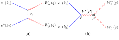
Figure 1: Feynman diagrams of $e^{+}e^{-}\to W^{+}W^{-}$, (a) $t$-channel and (b) $s$-channel with anomalous $W^{+}W^{-}V$ ($V=\gamma,Z$) vertex contribution shown by shaded blob.

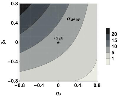
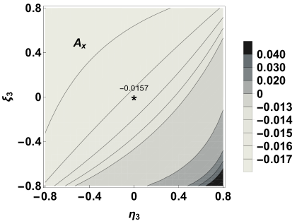
Figure 2: The production cross section $\sigma_{W^{+}W^{-}}$ in pb (left-panel) and the polarization asymmetry $A_{x}$ (right-panel) in the SM as a function of longitudinal beam polarizations $\eta_{3}$ (for $e^{-}$) and $\xi_{3}$ (for $e^{+}$) at $\sqrt{s}=500$ GeV. The asterisks represent the unpolarized points and the numbers near them correspond to the SM values for corresponding observables with unpolarized beams.

We study $W^{+}W^{-}$ production at ILC running at $\sqrt{s}=500$ GeV and integrated luminosity ${\cal L}=100$ fb^-1 using longitudinal polarization of $e^{-}$ and $e^{+}$ beams giving $50$ fb^-1 to each choice of beam polarization. The Feynman diagrams for the process are shown in Fig. 1 where Fig. 1(a) corresponds to the $\nu_{e}$ mediated $t$-channel diagram and the Fig. 1(b) corresponds to the $V~{}(Z/\gamma)$ mediated $s$-channel diagram containing the anomalous triple gauge boson couplings (aTGC) contributions represented by the shaded blob. The decay mode is chosen to be

$$W^{+}\to q_{u}~{}\bar{q}_{d}\ \ ,~{}~{}~{}~{}~{}W^{-}\to l^{-}~{}\bar{\nu}_{l},~{}~{}~{}l=e,\mu,$$ (9)

where $q_{u}$ and $q_{d}$ are up-type and down-type quarks, respectively. We use complete set of eight spin-$1$ observables of $W^{-}$ boson  Aguilar-Saavedra:2015yza ; Rahaman:2016pqj .

The $W$ boson being a spin-$1$ particle, its normalized production density matrix in the spin basis can be written as Bourrely:1980mr ; Boudjema:2009fz

$$\rho(\lambda,\lambda^{\prime})=\dfrac{1}{3}\Bigg{[}I_{3\times 3}+\dfrac{3}{2}\vec{p}.\vec{S}+\sqrt{\dfrac{3}{2}}T_{ij}\big{(}S_{i}S_{j}+S_{j}S_{i}\big{)}\Bigg{]},$$ (10)

where $\vec{p}=\{p_{x},p_{y},p_{z}\}$ is the vector polarization of a spin-$1$ particle, $\vec{S}=\{S_{x},S_{y},S_{z}\}$ is the spin basis and $T_{ij}~{}(i,j=x,y,z)$ is the $2^{nd}$-rank symmetric traceless tensor, and $\lambda$ and $\lambda^{\prime}$ are helicities of the particle. The tensor $T_{ij}$ has five independent elements, which are $T_{xy}$, $T_{xz}$, $T_{yz}$, $T_{xx}-T_{yy}$ and $T_{zz}$. Combining the $\rho(\lambda,\lambda^{\prime})$ with the normalized decay density matrix of the particle to a pair of fermion $f$, the differential cross section would be Boudjema:2009fz

$$\frac{1}{\sigma}\ \frac{d\sigma}{d\Omega_{f}} = \frac{3}{8\pi}\left[\left(\frac{2}{3}-(1-3\delta)\ \frac{T_{zz}}{\sqrt{6}}\right)+\alpha\ p_{z}\cos\theta_{f}\right.$$ (11)

$$+ \sqrt{\frac{3}{2}}(1-3\delta)\ T_{zz}\cos^{2}\theta_{f}$$

$$+ \left(\alpha\ p_{x}+2\sqrt{\frac{2}{3}}(1-3\delta)\ T_{xz}\cos\theta_{f}\right)\sin\theta_{f}\ \cos\phi_{f}$$

$$+ \left(\alpha\ p_{y}+2\sqrt{\frac{2}{3}}(1-3\delta)\ T_{yz}\cos\theta_{f}\right)\sin\theta_{f}\ \sin\phi_{f}$$

$$+ (1-3\delta)\left(\frac{T_{xx}-T_{yy}}{\sqrt{6}}\right)\sin^{2}\theta_{f}\cos(2\phi_{f})$$

$$+ \left.\sqrt{\frac{2}{3}}(1-3\delta)\ T_{xy}\ \sin^{2}\theta_{f}\ \sin(2\phi_{f})\right].$$

Here $\theta_{f}$, $\phi_{f}$ are the polar and the azimuthal orientation of the fermion $f$, in the rest frame of the particle ($W$) with its would-be momentum along the $z$-direction. The initial beam direction and the $W^{-}$ momentum in the lab frame define the $x$–$z$ plane, i.e. $\phi=0$ plane, in the rest frame of $W^{-}$ as well. In this case $\alpha=-1$ and $\delta=0$. The vector polarizations $\vec{p}$ and independent tensor polarizations $T_{ij}$ are calculable from the asymmetries constructed from the decay angular distribution of the lepton (here $l^{-}$). For example $p_{x}$ can be calculated from the asymmetry $A_{x}$ as

$$A_{x}=\dfrac{\sigma(\cos\phi_{f}>0)-\sigma(\cos\phi_{f}<0)}{\sigma(\cos\phi_{f}>0)+\sigma(\cos\phi_{f}<0)}\equiv\frac{3\alpha p_{x}}{4}.$$ (12)

The asymmetries corresponding to all other polarizations, vector polarizations $p_{y}$, $p_{z}$ and independent tensor polarizations $T_{ij}$ are $A_{y}$, $A_{z}$, $A_{xy}$, $A_{xz}$, $A_{yz}$, $A_{x^{2}-y^{2}}$, $A_{zz}$; see Ref. Rahaman:2016pqj for details.

Owing to the $t$-channel process (Fig. 1a) and absence of a $u$-channel process, like in $ZV$ production Rahaman:2016pqj ; Rahaman:2017qql , the $W^{\pm}$ produced are not forward-backward symmetric. We include the forward-backward asymmetry of $W^{-}$, defined as

$$A_{fb}=\frac{1}{\sigma_{W^{+}W^{-}}}\Bigg{[}\int_{0}^{1}\frac{d\sigma_{W^{+}W^{-}}}{d\cos\theta_{W^{-}}}-\int_{-1}^{0}\frac{d\sigma_{W^{+}W^{-}}}{d\cos\theta_{W^{-}}}\Bigg{]},$$ (13)

to the set of observables making a total of ten observables including the cross section as well. Here $\theta_{W^{-}}$ is the production angle of the $W^{-}$ with respect to the $e^{-}$ beam direction and $\sigma_{W^{+}W^{-}}$ is the production cross section.

These asymmetries can be measured in a real collider from the final state lepton $l^{-}$. One has to calculate the asymmetries in the rest frame of $W^{-}$ which require the missing $\bar{\nu_{l}}$ momenta to be reconstructed. At an $e^{+}$ $e^{-}$ collider, as studied here, reconstructing the missing $\bar{\nu_{l}}$ is possible because only one missing particle is involved and no parton distribution functions (PDFs) are involved, i.e., initial momenta are known. But for a collider where PDFs are involved, reconstructing the actual missing momenta may not be possible.

We explore the dependence of the cross section and asymmetries on the longitudinal polarization $\eta_{3}$ of $e^{-}$ and $\xi_{3}$ of $e^{+}$. In Fig. 2, we show the production cross section $\sigma_{W^{+}W^{-}}$ and $A_{x}$ as a function of beam polarizations as an example. The cross section decreases along the $\eta_{3}=-\xi_{3}$ path from $20$ pb on the left-top corner to $7.2$ pb at the unpolarized point and further to $1$ pb in the right-bottom corner. This is because of the $W^{\pm}$ couples to the left chiral $e^{-}$ i.e., it requires $e^{-}$ to be negatively polarized and $e^{+}$ to be positively polarized for the higher cross section. The variation of $A_{fb}$ (not shown) with the beam polarization is the same as the cross section but very slow above the line $\eta_{3}=\xi_{3}$. From this, we can expect that a positive $\eta_{3}$ and a negative $\xi_{3}$ will reduce the SM contributions to observables increasing the $S/\sqrt{B}$ ratio ($S=$ signal, $B=$ background). Some other asymmetries, like $A_{x}$, have the opposite dependence on the beam polarizations compared to the cross section; their modulus reduce for negative $\eta_{3}$ and positive $\xi_{3}$.

III Probe to the anomalous couplings

Figure 3: The $WWV$ vertex showing anomalous contribution represented by the shaded blob on top of SM. The momentum $P$ is incoming to the vertex, while $q$ and $\bar{q}$ are outgoing from the vertex.

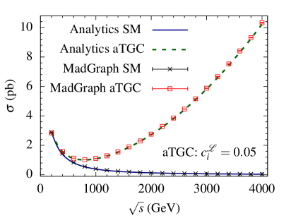
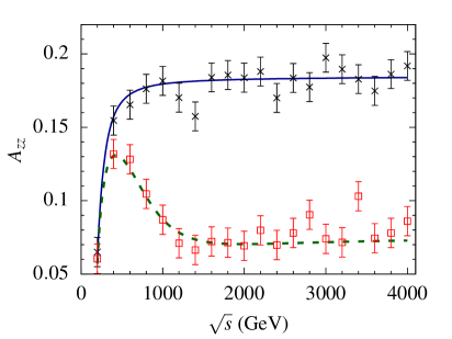
Figure 4: The cross section $\sigma$ including the decays in pb (left-panel) and the asymmetry $A_{zz}$ (right-panel) in the SM and aTGC with all anomalous couplings ($c_{i}^{\cal L}$) at $0.05$ as a function of $\sqrt{s}$ for the SM analytic (solid/blue) and aTGC analytic (dashed /green) with unpolarized beams. The crossed (black) points and boxed (red) points with the error bar correspond to results from MadGraph5. The error bars are given for number of events of $10^{4}$.

The $W^{+}W^{-}V$ vertex (Fig. 3) for the Lagrangian in Eq. (4) for on-shell $W$s would be $ig_{WWV}\Gamma_{V}^{\mu\alpha\beta}$ Gaemers:1978hg ; Hagiwara:1986vm and it is given by

$$\Gamma_{V}^{\mu\alpha\beta} = f_{1}^{V}(q-\bar{q})^{\mu}g^{\alpha\beta}-\frac{f_{2}^{V}}{m_{W}^{2}}(q-\bar{q})^{\mu}P^{\alpha}P^{\beta}$$ (14)

$$+f_{3}^{V}(P^{\alpha}g^{\mu\beta}-P^{\beta}g^{\mu\alpha})+if_{4}^{V}(P^{\alpha}g^{\mu\beta}+P^{\beta}g^{\mu\alpha})$$

$$+if_{5}^{V}\epsilon^{\mu\alpha\beta\rho}(q-\bar{q})_{\rho}-f_{6}^{V}\epsilon^{\mu\alpha\beta\rho}P_{\rho}$$

$$+\frac{\widetilde{f_{7}^{V}}}{m_{W}^{2}}\left(\bar{q}^{\alpha}\epsilon^{\mu\beta\rho\sigma}+q^{\beta}\epsilon^{\mu\alpha\rho\sigma}\right)q_{\rho}\bar{q}_{\sigma},$$

where $P,q,\bar{q}$ are the four-momenta of $V,W^{-},W^{+}$, respectively. The momentum conventions are shown in Fig. 3. The form factors $f_{i}$s have been obtained from the Lagrangian in Eq. (4) using FeynRules Alloul:2013bka to be

$$f_{1}^{V}=g_{1}^{V}+\frac{\hat{s}}{2m_{W}^{2}}\lambda^{V},\hskip 5.69046ptf_{2}^{V}=\lambda^{V},\hskip 5.69046ptf_{3}^{V}=g_{1}^{V}+\kappa^{V}+\lambda^{V},$$

$$f_{4}^{V}=g_{4}^{V},\hskip 5.69046ptf_{5}^{V}=g_{5}^{V},\hskip 5.69046ptf_{6}^{V}=\widetilde{\kappa^{V}}+\left(1-\frac{\hat{s}}{2m_{W}^{2}}\right)\widetilde{\lambda^{V}},$$

$$\widetilde{f_{7}^{V}}=\widetilde{\lambda^{V}}.$$ (15)

We use the vertex factors in Eq. (14) for the analytical calculation of our observables and cross validate them numerically with MadGraph5 Alwall:2014hca implementation of Eq. (4). As an example, we present two observables $\sigma_{W^{+}W^{-}}$ and $A_{zz}$ for the SM ($c_{i}^{\cal L}=0.0$) and for a chosen couplings point $c_{i}^{\cal L}=0.05$, in Fig. 4. The agreement between the analytical and the numerical calculations over a range of $\sqrt{s}$ indicates the validity of relations in Eq. (III), especially the $s$ dependence of $f_{1}^{V}$ and $f_{6}^{V}$.

Analytical expressions of all the observables have been obtained and their dependence on the anomalous couplings $c_{i}^{\cal L}$ are given in Table 5 in appendix A. The $CP$-even couplings in $CP$-even observables $\sigma$, $A_{x}$, $A_{z}$, $A_{xz}$ , $A_{x^{2}-y^{2}}$, and $A_{zz}$ appear in linear as well as in quadratic form but do not appear in the $CP$-odd observables $A_{y}$, $A_{xy}$, and $A_{yz}$. On the other hand, $CP$-odd couplings appear linearly in $CP$-odd observables and quadratically in $CP$-even observables. Thus the $CP$-even couplings may have a double patch in their confidence interval leading to asymmetric limits which will be discussed in Sect. III.1. On the other hand, the $CP$-odd couplings will have a single patch in their confidence interval and will pose symmetric limits.

III.1 Sensitivity of observables on anomalous couplings and their binning

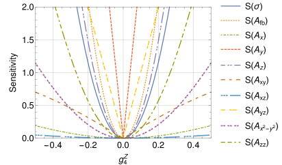
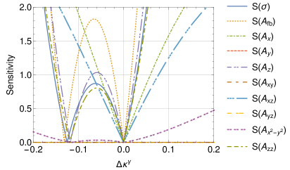
Figure 5: The one-parameter sensitivities of cross section $\sigma$, $A_{fb}$ and the eight polarization asymmetries ($A_{i}$) on $g_{4}^{Z}$ (left-panel) and on $\Delta\kappa^{\gamma}$ (right-panel) for $\sqrt{s}=500$ GeV, ${\cal L}=100$ fb^-1 with unpolarized beams.

The sensitivity of an observable ${\cal O}$ depending on anomalous couplings $\vec{f}$ with beam polarization $\eta_{3}$, $\xi_{3}$ is given by

$$S{\cal O}(\vec{f},\eta_{3},\xi_{3})=\dfrac{|{\cal O}(\vec{f},\eta_{3},\xi_{3})-{\cal O}(\vec{0},\eta_{3},\xi_{3})|}{|\delta{\cal O}(\eta_{3},\xi_{3})|},$$ (16)

where $\delta{\cal O}=\sqrt{(\delta{\cal O}_{stat.})^{2}+(\delta{\cal O}_{sys.})^{2}}$ is the estimated error in ${\cal O}$. The error for the cross section would be,

$$\delta\sigma(\eta_{3},\xi_{3})=\sqrt{\frac{\sigma(\eta_{3},\xi_{3})}{{\cal L}}+\epsilon_{\sigma}^{2}\sigma(\eta_{3},\xi_{3})^{2}}$$ (17)

whereas the estimated error in the asymmetries would be,

$$\delta A(\eta_{3},\xi_{3})=\sqrt{\frac{1-A(\eta_{3},\xi_{3})^{2}}{{\cal L}\sigma(\eta_{3},\xi_{3})}+\epsilon_{A}^{2}}.$$ (18)

Here ${\cal L}$ is the luminosity of the data set, $\epsilon_{\sigma}$, and $\epsilon_{A}$ are the systematic fractional errors in the cross section and asymmetries, respectively. We take ${\cal L}=50$ fb^-1 for each choice of beam polarizations, $\epsilon_{\sigma}=2~{}\%$ and $\epsilon_{A}=1~{}\%$, as a benchmark scenario for the present analyses. The sensitivity of all $10$ observables have been studied on all $14$ couplings of the Lagrangian in Eq. (4) with the chosen $\sqrt{s}$, ${\cal L}$ and systematic uncertainties. The sensitivity of all observables on $g_{4}^{Z}$ and $\Delta\kappa^{\gamma}$ are shown in Fig. 5 as representative. Being $CP$-odd (either only linear or only quadratic terms present), $g_{4}^{Z}$ has a single patch in the confidence interval, while the $\Delta\kappa^{\gamma}$ being $CP$-even (linear as well as quadratic terms present), has two patches in the sensitivity curve, as noted earlier. The $CP$-odd observable $A_{y}$ provides the tightest one-parameter limit on $g_{4}^{Z}$. The tightest $1\sigma$ limit on $\Delta\kappa^{\gamma}$ is obtained using $A_{fb}$, while at $2\sigma$ level, a combination of $A_{fb}$ and $A_{x}$ provide the tightest limit.

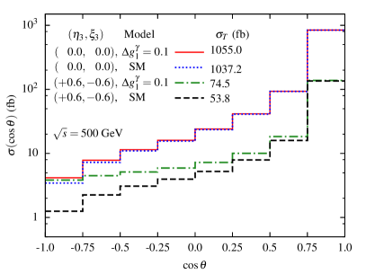
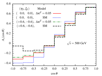
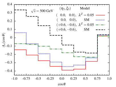
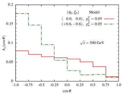
Figure 6: The cross section $\sigma$ (left-top), $A_{z}$ (right-top), $A_{x}$ (left-bottom) and $A_{y}$ (right-bottom) as a function of $\cos\theta$ of $W^{-}$ in $8$ bins for $\sqrt{s}=500$ GeV. The dotted (blue) lines correspond to the SM unpolarized values, solid (red) lines correspond to the unpolarized aTGC values, dashed (black) lines represent polarized SM values, and dashed-dotted (green) lines represent polarized aTGC values of observables. For aTGC, only one anomalous coupling has been assumed nonzero and others kept at zero in each panel.

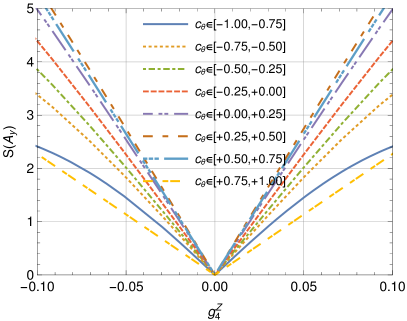
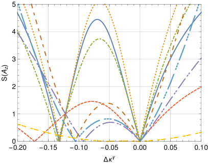
Figure 7: The one-parameter sensitivities of $A_{x}$ on $g_{4}^{Z}$ (left-panel) and of $A_{z}$ on $\Delta\kappa^{\gamma}$ (right-panel) in eight bins at $\sqrt{s}=500$ GeV, ${\cal L}=100$ fb^-1 with $c_{\theta}=\cos\theta_{W^{-}}$ for unpolarized beams.

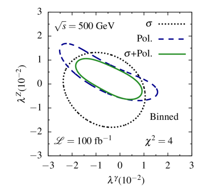
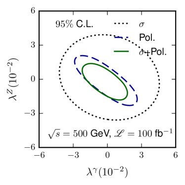
Figure 8: The $\chi^{2}=4$ contours in the left-panel and $95~{}\%$ C.L. contours from simultaneous analysis in the right-panel in the $\lambda^{\gamma}$–$\lambda^{Z}$ plane using the binned cross sections ($\sigma$) alone in dotted (black) lines, just binned polarizations asymmetries (Pol.) in dashed (blue) lines and the binned cross sections together with binned polarization asymmetries ($\sigma$ + Pol.) in solid (green) lines for $\sqrt{s}=500$ GeV, ${\cal L}=100$ fb^-1.

Here, we have a total of $14$ different anomalous couplings to be measured, while we only have $10$ observables. A certain combination of large couplings may mimic the SM within the statistical errors. To avoid these, we need more observables to be included in the analysis. We achieve this by dividing $\cos\theta_{W^{-}}$ into eight bins and calculate the cross section and polarization asymmetries in all of them. In Fig. 6, the cross section and the polarization asymmetries $A_{z}$, $A_{x}$, and $A_{y}$ are shown as a function of $\cos\theta_{W^{-}}$ for the SM and some aTGC couplings for both polarized and unpolarized beams. The SM values for unpolarized cases are shown in dotted (blue) lines, and the SM values with a polarization of $(\eta_{3},\xi_{3})=(+0.6,-0.6)$ are shown in dashed (black) lines. The solid (red) lines correspond to unpolarized aTGC values, while dashed-dotted (green) lines represent polarized aTGC values of observables. For the cross section (left-top-panel), we take $\Delta g_{1}^{\gamma}$ to be $0.1$ and all other couplings to zero for both polarized and unpolarized beams. We see that the fractional deviation from the SM value is larger in the most backward bin ($\cos\theta_{W^{-}}\in(-1.0,-0.75)$) and gradually reduces in the forward direction. The deviation is even larger in case of beam polarization. The sensitivity of the cross section on $\Delta g_{1}^{\gamma}$ is thus expected to be high in the most backward bin. In the case of asymmetries, $A_{z}$ (right-top-panel), $A_{xz}$ (left-bottom-panel) and $A_{y}$ (right-bottom-panel), the aTGC are assumed to be $\Delta\kappa^{Z}=0.05$, $\lambda^{Z}=0.05$ and $g_{4}^{Z}=0.05$, respectively, while others are kept at zero. The changes in the asymmetries due to aTGC are larger in the backward bin for both polarized and unpolarized beam cases. We note that the asymmetries may not have the highest sensitivity in the most backward bin but in some other bin. We consider the cross section and eight polarization asymmetries in all eight bins, i.e., we have $72$ observables in our analysis.

one-parameter sensitivities of the set of nine observables in all eight bins have been studied. We show the sensitivity of $A_{y}$ on $g_{4}^{Z}$ and of $A_{z}$ on $\Delta\kappa^{\gamma}$ in the eight bins in Fig. 7 as representative. The tightest limits based on the sensitivity (coming from one bin) is roughly twice as tight as compared to the unbinned case in Fig. 5. Thus, we expect simultaneous limits on all the couplings to be tighter when using binned observables.

Table 2: The list of analyses performed in the present work and set of observables used with different kinematical cuts to obtain simultaneous limits on the anomalous couplings at $\sqrt{s}=500$ GeV, ${\cal L}=100$ fb^-1 with unpolarized beams. The rectangular volumes of couplings at $95\%$ BCI are shown in the last column for each analyses (see text for details).

Analysis Name	Set of Observables	Kinematical Cut on $\cos\theta_{W^{-}}$	Volume of Limits
$\sigma$-unbinned	$\sigma$	$\cos\theta_{W^{-}}\in[-1.0,1.0]$	$4.4\times 10^{-11}$
Unbinned	$\sigma$, $A_{fb}$, $A_{i}$	$\cos\theta_{W^{-}}\in[-1.0,1.0]$	$3.1\times 10^{-12}$
$\sigma$-binned	$\sigma$	$\cos\theta_{W^{-}}\in[\frac{m-5}{4},\frac{m-4}{4}]$, $m=1,2,\dots,8$	$3.7\times 10^{-12}$
Pol.-binned	$A_{i}$	$\cos\theta_{W^{-}}\in[\frac{m-5}{4},\frac{m-4}{4}]$, $m=1,2,\dots,8$	$1.6\times 10^{-15}$
Binned	$\sigma$, $A_{i}$	$\cos\theta_{W^{-}}\in[\frac{m-5}{4},\frac{m-4}{4}]$, $m=1,2,\dots,8$	$5.2\times 10^{-17}$

We perform a set of Markov-chain–Monte-Carlo (MCMC) analyses with a different set of observables for different kinematical cuts with unpolarized beams to understand their roles in providing limits on the anomalous couplings. These analyses are listed in Table 2. The corresponding $14$-dimensional rectangular volume made out of $95\%$ Bayesian confidence interval (BCI) on the anomalous couplings are also listed in Table 2 in the last column. The simplest analysis would be to consider only the cross section in the full $\cos\theta_{W^{-}}$ domain and perform MCMC analysis which is named as $\sigma$-unbinned. The typical $95\%$ limits on the parameters range from $\sim\pm 0.04$ to $\pm 0.25$ giving the volume of limits to be $4.4\times 10^{-11}$. As we have polarizations asymmetries, the straight forward analysis would be to consider all the observables for the full domain of $\cos\theta_{W^{-}}$. This analysis is named Unbinned where limits on anomalous couplings get constrained better reducing the volume of limits by a factor of $10$ compared to the $\sigma$-unbinned. To see how binning improves the limits, we perform an analysis named $\sigma$-binned using only the cross section in eight bins. We see that the analysis $\sigma$-binned is better than the $\sigma$-unbinned and comparable to the analysis Unbinned. To see the strength of the polarization asymmetries, we perform an analysis named Pol.-binned using just the polarization asymmetries in eight bins. We see that this analysis is much better than the analysis $\sigma$-binned. The most natural and complete analysis would be to consider all the observables after binning. The analysis is named as Binned which has limits much better than any analysis. The comparison between the analyses, $\sigma$-binned, Pol.-binned, and Binned is shown in Fig. 8 in the panel $\lambda^{\gamma}$–$\lambda^{Z}$ in two-parameter (left-panel) as well as in multi-parameter (right-panel) analysis using MCMC as representative. The right-panel reflects Table 2. The behaviours are same even in the two parameter analysis (left-panel) by keeping all other parameter to zero, i.e, the bounded region for $\chi^{2}=4$ is smaller in Pol.-binned (Pol.) than $\sigma$-binned ($\sigma$) and smallest for Binned ($\sigma$+Pol.).

We also calculate one-parameter limits on all the couplings at $95~{}\%$ C.L. considering all the binned observables with unpolarized beams in the effective vertex formalism as well as in the effective operator approach and list them in the last column of Tables 3 & 4, respectively, for comparison. In the next subsection, we study the effect of beam polarizations on the limits of the anomalous couplings.

III.2 Effect of beam polarizations to the limits on the anomalous couplings

Table 3: List of posterior $95~{}\%$ BCI of anomalous couplings $c_{i}^{\cal L}$ ($10^{-2}$) of the Lagrangian in Eq. (4) at $\sqrt{s}=500$ GeV, ${\cal L}=100$ fb^-1 for a chosen set of longitudinal beam polarizations $\eta_{3}$ and $\xi_{3}$ from MCMC global fits in Binned case. The limits for the best choice of beam polarization within technological reach, i.e., $(\pm 0.8,\mp 0.6)$ are marked in bold. The pictorial visualization for these $95~{}\%$ BCI of $c_{i}^{\cal L}$ are shown in Fig. 9 in the left-panel. The one-parameter ($1P$) limits ($10^{-2}$) at $95~{}\%$ BCI with unpolarized beams are given in the last column for comparison. The notation used here is ${}_{low}^{high}\equiv[low,high]$ with $low$ being the lower limit and $high$ being the upper limit.

Parameter	$(0,0)$	$(\pm 0.2,\mp 0.2)$	$(\pm 0.4,\mp 0.4)$	$(\pm 0.6,\mp 0.6)$	$\mathbf{(\pm 0.8,\mp 0.6)}$	$(\pm 0.8,\mp 0.8)$	$1P$$(0,0)$
$\Delta g_{1}^{\gamma}$	${}_{-8.5}^{+5.5}$	${}_{-7.4}^{+3.3}$	${}_{-6.0}^{+2.7}$	${}_{-2.7}^{+2.1}$	$\mathbf{{}_{-2.3}^{+1.7}}$	${}_{-2.0}^{+1.6}$	${}_{-1.4}^{+1.3}$
$g_{4}^{\gamma}$	${}_{-6.0}^{+5.8}$	${}_{-5.4}^{+5.3}$	${}_{-4.0}^{+4.0}$	${}_{-3.0}^{+3.0}$	$\mathbf{{}_{-2.5}^{+2.5}}$	${}_{-2.2}^{+2.2}$	${}_{-1.9}^{+1.9}$
$g_{5}^{\gamma}$	${}_{-6.1}^{+6.1}$	${}_{-5.2}^{+5.1}$	${}_{-3.1}^{+2.6}$	${}_{-2.0}^{+1.4}$	$\mathbf{{}_{-1.6}^{+1.1}}$	${}_{-1.4}^{+1.0}$	${}_{-2.0}^{+1.9}$
$\lambda^{\gamma}$	${}_{-1.8}^{+1.4}$	${}_{-1.6}^{+1.2}$	${}_{-1.2}^{+1.2}$	${}_{-0.68}^{+1.0}$	$\mathbf{{}_{-0.61}^{+0.89}}$	${}_{-0.57}^{+0.81}$	${}_{-1.1}^{+0.77}$
$\widetilde{\lambda^{\gamma}}$	${}_{-1.6}^{+1.6}$	${}_{-1.4}^{+1.4}$	${}_{-1.1}^{+1.1}$	${}_{-0.88}^{+0.88}$	$\mathbf{{}_{-0.82}^{+0.82}}$	${}_{-0.78}^{+0.77}$	${}_{-1.0}^{+1.0}$
$\Delta\kappa^{\gamma}$	${}_{-5.7}^{+0.91}$	${}_{-4.4}^{+0.32}$	${}_{-4.3}^{+0.46}$	${}_{-0.69}^{+0.28}$	$\mathbf{{}_{-0.55}^{+0.27}}$	${}_{-0.48}^{+0.25}$	${}_{-0.34}^{+0.33}$
$\widetilde{\kappa^{\gamma}}$	${}_{-6.0}^{+6.1}$	${}_{-5.2}^{+5.2}$	${}_{-3.9}^{+4.0}$	${}_{-3.0}^{+2.9}$	$\mathbf{{}_{-2.6}^{+2.6}}$	${}_{-2.3}^{+2.3}$	${}_{-2.4}^{+2.3}$
$\Delta g_{1}^{Z}$	${}_{-3.7}^{+7.2}$	${}_{-2.8}^{+5.6}$	${}_{-2.6}^{+4.5}$	${}_{-2.0}^{+2.1}$	$\mathbf{{}_{-1.7}^{+1.8}}$	${}_{-1.5}^{+1.6}$	${}_{-1.3}^{+1.3}$
$g_{4}^{Z}$	${}_{-4.7}^{+4.8}$	${}_{-4.3}^{+4.3}$	${}_{-3.3}^{+3.3}$	${}_{-2.5}^{+2.5}$	$\mathbf{{}_{-2.2}^{+2.2}}$	${}_{-2.0}^{+2.0}$	${}_{-1.4}^{+1.4}$
$g_{5}^{Z}$	${}_{-4.8}^{+4.7}$	${}_{-4.1}^{+4.0}$	${}_{-2.3}^{+2.1}$	${}_{-1.5}^{+1.3}$	$\mathbf{{}_{-1.3}^{+1.0}}$	${}_{-1.2}^{+0.86}$	${}_{-1.3}^{+1.2}$
$\lambda^{Z}$	${}_{-1.5}^{+1.1}$	${}_{-1.3}^{+1.0}$	${}_{-1.1}^{+0.80}$	${}_{-0.94}^{+0.49}$	$\mathbf{{}_{-0.83}^{+0.47}}$	${}_{-0.76}^{+0.44}$	${}_{-0.57}^{+0.56}$
$\widetilde{\lambda^{Z}}$	${}_{-1.3}^{+1.3}$	${}_{-1.1}^{+1.1}$	${}_{-0.90}^{+0.90}$	${}_{-0.77}^{+0.77}$	$\mathbf{{}_{-0.73}^{+0.73}}$	${}_{-0.68}^{+0.68}$	${}_{-0.56}^{+0.57}$
$\Delta\kappa^{Z}$	${}_{-1.5}^{+3.6}$	${}_{-0.49}^{+3.2}$	${}_{-0.44}^{+3.1}$	${}_{-0.38}^{+0.56}$	$\mathbf{{}_{-0.35}^{+0.43}}$	${}_{-0.32}^{+0.36}$	${}_{-0.48}^{+0.43}$
$\widetilde{\kappa^{Z}}$	${}_{-5.0}^{+4.7}$	${}_{-4.2}^{+4.2}$	${}_{-3.3}^{+3.3}$	${}_{-2.5}^{+2.5}$	$\mathbf{{}_{-2.2}^{+2.2}}$	${}_{-2.0}^{+2.1}$	${}_{-1.5}^{+1.5}$

Table 4: The list of posterior $95~{}\%$ BCI of anomalous couplings $c_{i}^{\cal O}$ (TeV^-2) of effective operators in Eq. (I) and their translated limits on the couplings $c_{i}^{{\cal L}_{g}}$ ($10^{-2}$) for $\sqrt{s}=500$ GeV, ${\cal L}=100$ fb^-1 in the Binned case for a chosen set of longitudinal beam polarizations $\eta_{3}$ and $\xi_{3}$ from MCMC global fits. The pictorial visualization for these $95~{}\%$ BCI of $c_{i}^{\cal O}$ and $c_{i}^{{\cal L}_{g}}$ are shown in Fig. 9 in the right-top and right-bottom panels, respectively. The rest of the details are same as in Table 3.

Parameter	$(0,0)$	$(\pm 0.2,\mp 0.2)$	$(\pm 0.4,\mp 0.4)$	$(\pm 0.6,\mp 0.6)$	$\mathbf{(\pm 0.8,\mp 0.6)}$	$(\pm 0.8,\mp 0.8)$	$1P$$(0,0)$
$\frac{c_{WWW}}{\Lambda^{2}}$	${}_{-1.9}^{+1.3}$	${}_{-1.4}^{+1.2}$	${}_{-1.1}^{+1.2}$	${}_{-0.96}^{+1.1}$	$\mathbf{{}_{-1.0}^{+1.1}}$	${}_{-0.94}^{+1.0}$	${}_{-0.97}^{+0.84}$
$\frac{c_{W}}{\Lambda^{2}}$	${}_{-1.4}^{+5.0}$	${}_{-1.1}^{+4.6}$	${}_{-0.86}^{+0.83}$	${}_{-0.72}^{+0.58}$	$\mathbf{{}_{-0.73}^{+0.60}}$	${}_{-0.63}^{+0.55}$	${}_{-0.58}^{+0.55}$
$\frac{c_{B}}{\Lambda^{2}}$	${}_{-23.7}^{+2.7}$	${}_{-20.2}^{+1.9}$	${}_{-1.3}^{+0.98}$	${}_{-0.75}^{+0.62}$	$\mathbf{{}_{-0.64}^{+0.56}}$	${}_{-0.53}^{+0.47}$	${}_{-1.3}^{+1.2}$
$\frac{c_{\widetilde{WWW}}}{\Lambda^{2}}$	${}_{-1.4}^{+1.4}$	${}_{-1.1}^{+1.1}$	${}_{-0.97}^{+0.97}$	${}_{-0.93}^{+0.94}$	$\mathbf{{}_{-0.90}^{+0.91}}$	${}_{-0.87}^{+0.87}$	${}_{-0.98}^{+0.97}$
$\frac{c_{\widetilde{W}}}{\Lambda^{2}}$	${}_{-12.0}^{+2.1}$	${}_{-10.0}^{+9.8}$	${}_{-6.7}^{+6.6}$	${}_{-4.1}^{+4.2}$	$\mathbf{{}_{-3.2}^{+3.2}}$	${}_{-2.6}^{+2.6}$	${}_{-9.9}^{+10.1}$
$\lambda^{V}$	${}_{-0.79}^{+0.52}$	${}_{-0.58}^{+0.50}$	${}_{-0.46}^{+0.49}$	${}_{-0.40}^{+0.46}$	$\mathbf{{}_{-0.41}^{+0.45}}$	${}_{-0.39}^{+0.42}$	${}_{-0.40}^{+0.35}$
$\widetilde{\lambda^{V}}$	${}_{-0.60}^{+0.60}$	${}_{-0.45}^{+0.44}$	${}_{-0.40}^{+0.40}$	${}_{-0.38}^{+0.39}$	$\mathbf{{}_{-0.37}^{+0.37}}$	${}_{-0.36}^{+0.36}$	${}_{-0.41}^{+0.40}$
$\Delta\kappa^{\gamma}$	${}_{-6.4}^{+0.52}$	${}_{-5.1}^{+0.44}$	${}_{-0.38}^{+0.28}$	${}_{-0.32}^{+0.24}$	$\mathbf{{}_{-0.32}^{+0.25}}$	${}_{-0.28}^{+0.23}$	${}_{-0.61}^{+0.56}$
$\widetilde{\kappa^{\gamma}}$	${}_{-3.9}^{+3.9}$	${}_{-3.2}^{+3.2}$	${}_{-2.1}^{+2.1}$	${}_{-1.3}^{+1.3}$	$\mathbf{{}_{-1.0}^{+1.0}}$	${}_{-0.84}^{+0.84}$	${}_{-3.2}^{+3.2}$
$\Delta g_{1}^{Z}$	${}_{-0.59}^{+2.1}$	${}_{-0.45}^{+1.9}$	${}_{-0.36}^{+0.34}$	${}_{-0.30}^{+0.24}$	$\mathbf{{}_{-0.30}^{+0.25}}$	${}_{-0.26}^{+0.23}$	${}_{-0.24}^{+0.23}$
$\Delta\kappa^{Z}$	${}_{-0.73}^{+3.6}$	${}_{-0.45}^{+3.2}$	${}_{-0.33}^{+0.34}$	${}_{-0.24}^{+0.21}$	$\mathbf{{}_{-0.24}^{+0.21}}$	${}_{-0.20}^{+0.19}$	${}_{-0.30}^{+0.30}$
$\widetilde{\kappa^{Z}}$	${}_{-1.1}^{+1.1}$	${}_{-0.91}^{+0.92}$	${}_{-0.61}^{+0.62}$	${}_{-0.38}^{+0.38}$	$\mathbf{{}_{-0.30}^{+0.29}}$	${}_{-0.24}^{+0.24}$	${}_{-0.93}^{+0.92}$

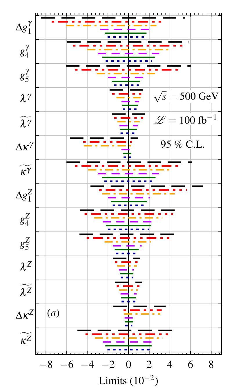
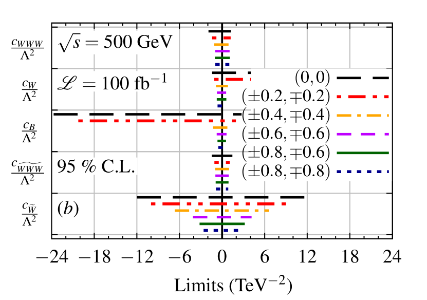
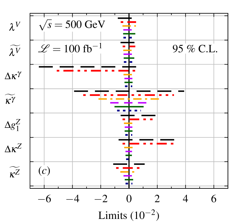
Figure 9: The pictorial visualizations of $95~{}\%$ BCI limits obtained from from MCMC global fits $(a):$ on the anomalous couplings $c_{i}^{\cal L}$ in the left-panel, $(b):$ on $c_{i}^{\cal O}$ in the right-top-panel and $(c):$ on $c_{i}^{{\cal L}_{g}}$ in the right-bottom-panel for $\sqrt{s}=500$ GeV, ${\cal L}=100$ fb^-1 using the binned observables. The numerical values of the limits can be read of in Tables 3 & 4.

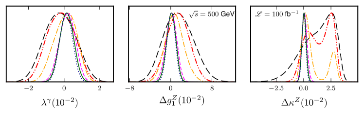
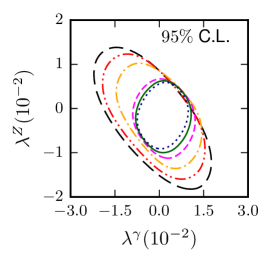
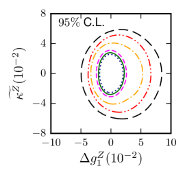
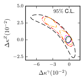
Figure 10: The marginalized $1D$ projections for the couplings $\lambda^{\gamma}$, $\Delta g_{1}^{Z}$ and $\Delta\kappa^{Z}$ in the top-panel and $2D$ projections at $95~{}\%$ C.L. on $\lambda^{\gamma}$–$\lambda^{Z}$, $\Delta g_{1}^{Z}$–$\widetilde{\kappa^{Z}}$ and $\Delta\kappa^{\gamma}$–$\Delta\kappa^{Z}$ planes in the bottom-panel from MCMC for a set of choice of beam polarizations are shown for $\sqrt{s}=500$ GeV, ${\cal L}=100$ fb^-1 using the binned observables in the effective vertex formalism. The legend labels are same as in Figs. 9 & 11.

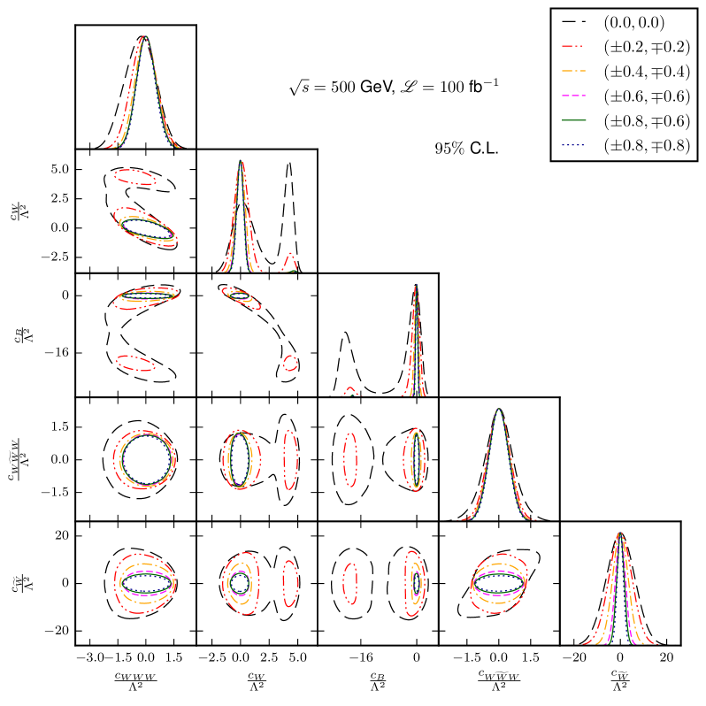
Figure 11: All the marginalized $1D$ projections and $2D$ projections at $95~{}\%$ C.L. from the MCMC in a triangular array for the effective operators (TeV^-2) for a set of choices of beam polarizations for $\sqrt{s}=500$ GeV, ${\cal L}=100$ fb^-1 using the binned observables.

We perform a MCMC analysis to estimate simultaneous limits on the anomalous couplings using the binned observables in both effective vertex formalism with $14$ independent couplings and an effective operator approach with five independent couplings for a set of chosen beam polarizations $(\eta_{3},\xi_{3})$ to be $(0,0)$, $(+0.2,-0.2)$, $(+0.4,-0.4)$, $(+0.6,-0.6)$, $(+0.8,-0.6)$, $(+0.8,-0.8)$ along with their opposite values. The beam polarization $(+\eta_{3},+\xi_{3})$ and its opposite $(-\eta_{3},-\xi_{3})$ are combined at the level of $\chi^{2}$ as

$$\chi^{2}_{tot}(\pm\eta_{3},\pm\xi_{3})=\sum_{bin}\sum_{N}\left(\chi^{2}\left[{\cal O}_{N}(+\eta_{3},+\xi_{3})\right]\right.$$

$$\left.+\chi^{2}\left[{\cal O}_{N}(-\eta_{3},-\xi_{3})\right]\right),$$ (19)

where $N$ runs over all the observables. The $95~{}\%$ BCI simultaneous limits for the chosen set of beam polarizations combined according to Eq. (III.2) are shown in Table 3 for effective vertex formalism ($c_{i}^{\cal L}$) and in Table 4 for effective operator approach ($c_{i}^{\cal O}$). The corresponding translated limit to the vertex factor couplings $c_{i}^{{\cal L}_{g}}$ are also shown in the Table 4 using relation from Eq. (5). While presenting limits the following notation is used

$${}_{low}^{high}\equiv[low,high]$$

with $low$ being lower limit and $high$ being upper limit. A pictorial visualization of the limits shown in Table 3 & and 4 is given in Fig. 9 for the easy comparisons. The limits on the couplings get tighter as the magnitude of the beam polarizations are increased along $\eta_{3}=-\xi_{3}$ path and become tightest at the extreme beam polarization $(\pm 0.8,\mp 0.8)$. However, the choice $(\pm 0.8,\mp 0.6)$ is best to put constraints on the couplings within the technological reach Vauth:2016pgg ; MoortgatPick:2006qp .

To show the effect of beam polarizations the marginalized $1D$ projection for the couplings $\lambda^{\gamma}$, $\Delta g_{1}^{Z}$ and $\Delta\kappa^{Z}$ as well as $2D$ projection at $95~{}\%$ C.L. on $\lambda^{\gamma}$–$\lambda^{Z}$, $\Delta g_{1}^{Z}$–$\widetilde{\kappa^{Z}}$ and $\Delta\kappa^{\gamma}$–$\Delta\kappa^{Z}$ planes are shown in Fig. 10 for the effective vertex formalism ($c_{i}^{\cal L}$) as representative. We observe that as the magnitude of beam polarizations are increased from $(0,0)$ to $(\pm 0.8,\mp 0.8)$ the contours get smaller centerd around the SM values in the $2D$ projection which is reflected in the $1D$ projection as well. In the $\Delta\kappa^{\gamma}$–$\Delta\kappa^{Z}$ panel, the contours get divided into two part at $(\pm 0.4,\mp 0.4)$ and become one single contour later centerd around the SM values. In the case of effective operator approach ($c_{i}^{\cal O}$), all the $1D$ and $2D$ ($95~{}\%$ C.L.) projections after marginalization are shown in Fig. 11. In this case the couplings $c_{W}$ and $c_{B}$ has two patches up-to beam polarization $(\pm 0.2,\mp 0.2)$ and become one single patch starting at beam polarization $(\pm 0.3,\mp 0.3)$ centerd around the SM values. As the magnitude of beam polarizations are increased along the $\eta_{3}=-\xi_{3}$ line, the measurement of the anomalous couplings gets improved. The set of beam polarizations chosen here are mostly along $\eta_{3}=-\xi_{3}$ line, but some choices off to the line might provide the same results. A discussion on the choice of beam polarization is given in the next subsection.

III.3 On the choice of beam polarizations

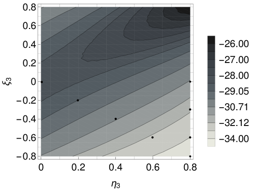
Figure 12: The averaged likelihood $L_{Av}=L(V_{\vec{f}}~{};\eta_{3},\xi_{3})$ in log scale as a function of $(\pm\eta_{3},\pm\xi_{3})$ in the effective vertex formalism for $\sqrt{s}=500$ GeV, ${\cal L}=100$ fb^-1.

In the previous subsection, we found that $(\pm\eta_{3},\pm\xi_{3})=(\pm 0.8,\pm 0.6)$ is the best choice of beam polarizations to provide simultaneous limits on the anomalous couplings obtained by MCMC analysis. Here, we discuss the average likelihood or the weighted volume of the parameter space defined as Rahaman:2017qql

$$L(V_{\vec{f}}~{};\eta_{3},\xi_{3}) = \int_{V_{\vec{f}}}\exp{\left[-\frac{1}{2}\chi_{tot}^{2}(\vec{f},\eta_{3},\xi_{3})\right]}d\vec{f}$$ (20)

to cross-examine the beam polarization choices made in the previous section. Here $\vec{f}$ is the coupling vector and $V_{\vec{f}}$ is the volume of parameter space over which the average is done and $L(V_{\vec{f}}~{};\eta_{3},\xi_{3})$ corresponds to the volume of the parameter space that is statistically consistent with the SM . One naively expects the limits to be tightest when $L(V_{\vec{f}}~{};\eta_{3},\xi_{3})$ is minimum. We calculate the above quantity as a function of $(\pm\eta_{3},\pm\xi_{3})$ for the Binned case in the effective vertex formalism given in the Lagrangian in Eq. (4) and present it in Fig. 12. As the opposite beam polarizations are combined, only the half-portions are shown in the $\eta_{3}$–$\xi_{3}$ plane. The dot ($\bullet$) points along the $\eta_{3}=-\xi_{3}$ are the chosen choice of beam polarizations for the MCMC analysis. We see that the average likelihood decreases along the $\eta_{3}=-\xi_{3}$ line while it increases along the $\eta_{3}=\xi_{3}$ line. The constant lines or contours of average likelihood in the figure imply that any beam polarizations along the lines/contours will provide the similar shape of $1D$ and $2D$ projections of couplings and their limits. For example, the point $(\pm 0.8,\mp 0.6)$ is equivalent to the point $(\pm 0.7,\mp 0.7)$ as well as $(\pm 0.6,\pm 0.8)$ roughly in providing simultaneous limits which are verified from the limits obtained by the MCMC analysis. From the figure, it is clear that the polarization $(\pm 0.8,\mp 0.6)$ is indeed the best choice to provide simultaneous limits on the anomalous couplings within the achievable range. However, the plan for polarization choices are $(\eta_{3},\xi_{3})=(0,0)$, $(\pm 0.8,0)$, $(\pm 0.8,\mp 0.3)$, and $(\pm 0.8,\mp 0.6)$ at the ILC Barklow:2015tja ; Bambade:2019fyw . These off-diagonal choices are equivalent to the diagonal choices we have used as Fig. 12 indicates. The polarization choice $(\pm 0.8,0)$ is equivalent to $(\pm 0.4,\mp 0.4)$ in providing limits on the couplings, while $(\pm 0.8,\mp 0.3)$ is equivalent to $(\pm 0.6,\mp 0.6)$ ($(\pm 0.57,\mp 0.57)$ to be precise). For completeness we also show the limits on the couplings for the off-diagonal polarization choices $(\pm 0.8,0)$ and $(\pm 0.8,\mp 0.3)$ in Table 6 on column $3$ and $5$, respectively in appendix A in the $SU(2)\times U(1)$ gauge for ${\cal L}=100$ fb^-1. By comparing Tables 4 and 6, one can confirm that the polarization choices $(\pm 0.8,0)$ and $(\pm 0.8,\mp 0.3)$ are indeed equivalent to the choices $(\pm 0.4,\mp 0.4)$ and $(\pm 0.6,\mp 0.6)$, respectively. We also obtain limits on the couplings in the $SU(2)\times U(1)$ gauge for the projected plan of the ILC Barklow:2015tja : polarization $(0,0)$ and $(\pm 0.8,0)$ at ${\cal L}=4$ ab^-1, polarization $(\pm 0.8,\mp 0.3)$ and $(\pm 0.8,\mp 0.6)$ at ${\cal L}=3.2$ ab^-1 and show them in Table 6. Increasing the luminosity from $100$ fb^-1 to the projected luminosity $3.2/4$ ab^-1 the limits on the couplings do not increase proportionately to the luminosity due to the systematic error considered here. If the systematic error is improved, we expect better limits on the couplings; e.g., with no systematic error, the limits can be further improved by a factor of $4$ at the projected luminosity.

IV Conclusion

In conclusion, we studied anomalous triple gauge boson couplings in $e^{+}e^{-}\to W^{+}W^{-}$ with longitudinally polarized beams using $W$ boson polarization observables together with the total cross section and the forward-backward asymmetry for $\sqrt{s}=500$ GeV and luminosity of ${\cal L}=100$ fb^-1. We have $14$ anomalous couplings, whereas we have only $10$ observables to measure them. So we binned all the observables ($A_{fb}$ excluded) in eight regions of the $\cos\theta_{W^{-}}$ to increase the number of observables to measure the couplings. We estimated the simultaneous limit on all the couplings for several chosen sets of beam polarization in both the effective vertex formalism and effective operator approach. The limits on the couplings are tighter when $SU(2)\times U(1)$ symmetry is assumed. We show the consistency between the best choice of beam polarizations and minimum likelihood averaged over the anomalous couplings. We find the polarization $(\pm 0.8,\mp 0.6)$ to be the best to provide the tightest constraint on the anomalous couplings at the ILC within the technological reach for both $100$ fb^-1 and $3.2$ ab^-1 of luminosity. Our one-parameter limits with unpolarized beams and simultaneous limits for the best polarization choice at $100$ fb^-1 are already much better than the one-parameter limits from experiments; see Table 4. Our analysis considers certain simplifying assumptions, such as the absence of initial-state/final-state radiation and detector effects. While the former might dilute the limits by a small amount, the latter is expected to have no effects on the results as only the leptonic channel is assumed and no falvor tagging or reconstruction is required.

Acknowledgements The authors thank Prof. Kaoru Hagiwara for useful discussions. R.R. thanks the Department of Science and Technology, Government of India for support through the DST-INSPIRE Fellowship for doctoral program, INSPIRE CODE IF140075, 2014. R.K.S. acknowledges SERB, DST, Government of India through the project EMR/2017/002778.

Appendix A The dependences of observables on anomalous couplings $c_{i}^{\cal L}$ and limits on the couplings $c_{i}^{\cal O}/c_{i}^{{\cal L}_{g}}$ to the projected plan of the ILC

The anomalous gauge boson couplings $c_{i}^{\cal O}$ of the effective operator in Eq. (I), the couplings $c_{i}^{\cal L}$ of the Lagrangian in Eq. (4), and the couplings $c_{i}^{{\cal L}_{g}}$ of the Lagrangian in the $SU(2)\times U(1)$ gauge (given in Eq. (5)) are labelled as

$$c_{i}^{\cal O} = \{c_{WWW},c_{W},c_{B},c_{\widetilde{WWW}},c_{\widetilde{W}}\},$$ (21)

$$c_{i}^{\cal L} = \{\Delta g_{1}^{V},g_{4}^{V},g_{5}^{V},\lambda^{V},\widetilde{\lambda^{V}},\Delta\kappa^{V},\widetilde{\kappa^{V}}\},~{}~{}~{}V=\gamma,Z,$$ (22)

$$c_{i}^{{\cal L}_{g}} = \{\lambda^{V},\widetilde{\lambda^{V}},\Delta\kappa^{\gamma},\widetilde{\kappa^{\gamma}},\Delta g_{1}^{Z},\Delta\kappa^{Z},\widetilde{\kappa^{Z}}\}.$$ (23)

The dependences of the observables on the anomalous couplings $c_{i}^{\cal L}$ are given in Table 5. The limits on the couplings $c_{i}^{\cal O}$ and $c_{i}^{{\cal L}_{g}}$ to the projected plan of the ILC are given in Table 6.

Table 5: The dependence of observables (numerators) on the anomalous couplings in the form of $c_{i}^{\cal L}$ (linear), $(c_{i}^{\cal L})^{2}$ (quadratic) and $c_{i}^{\cal L}c_{j}^{\cal L},~{}i\neq j$ (interference) in the process $e^{+}e^{-}\to W^{+}W^{-}$. Here, $V\in\{\gamma,Z\}$. The “✓" (check mark) represents the presence and “—" (big-dash) corresponds to absence.

Parameters	$\sigma$	$\sigma\times A_{x}$	$\sigma\times A_{y}$	$\sigma\times A_{z}$	$\sigma\times A_{xy}$	$\sigma\times A_{xz}$	$\sigma\times A_{yz}$	$\sigma\times A_{x^{2}-y^{2}}$	$\sigma\times A_{zz}$	$\sigma\times A_{fb}$
$\Delta g_{1}^{V}$	✓	✓	—	✓	—	✓	—	✓	✓	✓
$g_{4}^{V}$	—	—	✓	—	✓	—	✓	—	—	—
$g_{5}^{V}$	✓	✓	—	✓	—	✓	—	✓	✓	✓
$\lambda^{V}$	✓	✓	—	✓	—	✓	—	✓	✓	✓
$\widetilde{\lambda^{V}}$	—	—	✓	—	✓	—	✓	—	—	—
$\Delta\kappa^{V}$	✓	✓	—	✓	—	✓	—	✓	✓	✓
$\widetilde{\kappa^{V}}$	—	—	✓	—	✓	—	✓	—	—	—
$(\Delta g_{1}^{V})^{2}$	✓	✓	—	—	—	—	—	✓	✓	—
$(g_{4}^{V})^{2}$	✓	—	—	—	—	—	—	✓	✓	—
$(g_{5}^{V})^{2}$	✓	—	—	—	—	—	—	✓	✓	—
$(\lambda^{V})^{2}$	✓	✓	—	—	—	—	—	✓	✓	—
$(\widetilde{\lambda^{V}})^{2}$	✓	✓	—	—	—	—	—	✓	✓	—
$(\Delta\kappa^{V})^{2}$	✓	✓	—	—	—	—	—	✓	✓	—
$(\widetilde{\kappa^{V}})^{2}$	✓	✓	—	—	—	—	—	✓	✓	—
$\Delta g_{1}^{V}g_{4}^{V}$	—	—	—	—	—	—	✓	—	—	—
$\Delta g_{1}^{V}g_{5}^{V}$	—	—	—	✓	—	—	—	—	—	✓
$\Delta g_{1}^{V}\lambda^{V}$	✓	✓	—	—	—	—	—	✓	✓	—
$\Delta g_{1}^{V}\widetilde{\lambda^{V}}$	—	—	✓	—	✓	—	—	—	—	—
$\Delta g_{1}^{V}\Delta\kappa^{V}$	✓	✓	—	—	—	—	—	✓	✓	—
$\Delta g_{1}^{V}\widetilde{\kappa^{V}}$	—	—	✓	—	✓	—	—	—	—	—
$g_{4}^{V}g_{5}^{V}$	—	—	—	—	✓	—	—	—	—	—
$g_{4}^{V}\lambda^{V}$	—	—	—	—	—	—	✓	—	—	—
$g_{4}^{V}\widetilde{\lambda^{V}}$	—	—	—	✓	—	✓	—	—	—	✓
$g_{4}^{V}\Delta\kappa^{V}$	—	—	—	—	—	—	✓	—	—	—
$g_{4}^{V}\widetilde{\kappa^{V}}$	—	—	—	✓	—	✓	—	—	—	✓
$g_{5}^{V}\lambda^{V}$	—	—	—	✓	—	✓	—	—	—	✓
$g_{5}^{V}\widetilde{\lambda^{V}}$	—	—	—	—	—	—	✓	—	—	—
$g_{5}^{V}\Delta\kappa^{V}$	—	—	—	✓	—	✓	—	—	—	✓
$g_{5}^{V}\widetilde{\kappa^{V}}$	—	—	—	—	—	—	✓	—	—	—
$\lambda^{V}\widetilde{\lambda^{V}}$	—	—	✓	—	✓	—	—	—	—	—
$\lambda^{V}\Delta\kappa^{V}$	✓	✓	—	—	—	—	—	✓	✓	—
$\lambda^{V}\widetilde{\kappa^{V}}$	—	—	✓	—	✓	—	—	—	—	—
$\widetilde{\lambda^{V}}\Delta\kappa^{V}$	—	—	✓	—	✓	—	—	—	—	—
$\widetilde{\lambda^{V}}\widetilde{\kappa^{V}}$	✓	✓	—	—	—	—	—	✓	✓	—
$\Delta\kappa^{V}\widetilde{\kappa^{V}}$	—	—	✓	—	✓	—	—	—	—	—

Table 6: The list of posterior $95~{}\%$ BCI of anomalous couplings $c_{i}^{\cal O}$ (TeV^-2) of effective operators in Eq. (I) and their translated limits on the couplings $c_{i}^{{\cal L}_{g}}$ ($10^{-2}$) for $\sqrt{s}=500$ GeV and set of luminosities and beam polarizations (ILC projected) in Binned case from MCMC with the same notation used in Table 3.

$(\eta_{3},\xi_{3})$	$(0.0,0.0)$	$(\pm 0.8,0)$		$(\pm 0.8,\mp 0.3)$		$(\pm 0.8,\mp 0.6)$
${\cal L}$	$4$ ab-1	$100$ fb-1	$4$ ab-1	$100$ fb-1	$3.2$ ab-1	$3.2$ ab-1
$\frac{c_{WWW}}{\Lambda^{2}}$	${}_{-0.52}^{+0.44}$	${}_{-1.1}^{+1.2}$	${}_{-0.41}^{+0.41}$	${}_{-1.0}^{+1.1}$	${}_{-0.41}^{+0.42}$	${}_{-0.41}^{+0.42}$
$\frac{c_{W}}{\Lambda^{2}}$	${}_{-0.50}^{+0.59}$	${}_{-0.85}^{+0.70}$	${}_{-0.29}^{+0.27}$	${}_{-0.75}^{+0.59}$	${}_{-0.28}^{+0.26}$	${}_{-0.27}^{+0.25}$
$\frac{c_{B}}{\Lambda^{2}}$	${}_{-1.1}^{+0.81}$	${}_{-1.1}^{+0.81}$	${}_{-0.25}^{+0.23}$	${}_{-0.77}^{+0.64}$	${}_{-0.20}^{+0.19}$	${}_{-0.17}^{+0.16}$
$\frac{c_{\widetilde{WWW}}}{\Lambda^{2}}$	${}_{-0.35}^{+0.35}$	${}_{-1.0}^{+1.1}$	${}_{-0.37}^{+0.37}$	${}_{-0.97}^{+0.96}$	${}_{-0.38}^{+0.38}$	${}_{-0.37}^{+0.38}$
$\frac{c_{\widetilde{W}}}{\Lambda^{2}}$	${}_{-3.8}^{+3.9}$	${}_{-5.7}^{+5.9}$	${}_{-1.3}^{+1.3}$	${}_{-4.2}^{+4.3}$	${}_{-0.97}^{+0.97}$	${}_{-0.69}^{+0.69}$
$\lambda^{\gamma}$	${}_{-0.21}^{+0.18}$	${}_{-0.47}^{+0.51}$	${}_{-0.17}^{+0.17}$	${}_{-0.42}^{+0.47}$	${}_{-0.17}^{+0.18}$	${}_{-0.17}^{+0.17}$
$\widetilde{\lambda^{\gamma}}$	${}_{-0.15}^{+0.14}$	${}_{-0.43}^{+0.43}$	${}_{-0.15}^{+0.15}$	${}_{-0.40}^{+0.40}$	${}_{-0.16}^{+0.16}$	${}_{-0.16}^{+0.16}$
$\Delta\kappa^{\gamma}$	${}_{-0.21}^{+0.15}$	${}_{-0.38}^{+0.27}$	${}_{-0.11}^{+0.11}$	${}_{-0.33}^{+0.24}$	${}_{-0.12}^{+0.11}$	${}_{-0.11}^{+0.10}$
$\widetilde{\kappa^{\gamma}}$	${}_{-1.2}^{+1.3}$	${}_{-1.9}^{+1.9}$	${}_{-0.42}^{+0.42}$	${}_{-1.4}^{+1.4}$	${}_{-0.31}^{+0.31}$	${}_{-0.22}^{+0.22}$
$\Delta g_{1}^{Z}$	${}_{-0.21}^{+0.25}$	${}_{-0.35}^{+0.29}$	${}_{-0.12}^{+0.11}$	${}_{-0.31}^{+0.25}$	${}_{-0.12}^{+0.11}$	${}_{-0.11}^{+0.10}$
$\Delta\kappa^{Z}$	${}_{-0.23}^{+0.29}$	${}_{-0.30}^{+0.28}$	${}_{-0.10}^{+0.10}$	${}_{-0.25}^{+0.22}$	${}_{-0.092}^{+0.087}$	${}_{-0.085}^{+0.080}$
$\widetilde{\kappa^{Z}}$	${}_{-0.36}^{+0.35}$	${}_{-0.55}^{+0.54}$	${}_{-0.12}^{+0.12}$	${}_{-0.39}^{+0.39}$	${}_{-0.089}^{+0.090}$	${}_{-0.064}^{+0.064}$

Appendix B Note on linear approximation

If the cross section $\sigma$ is express as a function of couplings $c_{i}$ as,

$$\sigma=\sigma_{0}+\sum_{i}\sigma_{i}\times c_{i}+\sum_{i,j}\sigma_{ij}\times c_{i}c_{j},$$ (24)

linear approximation for the BSM operator will be possible if the quadratic contributions are much smaller than the linear contribution, i.e.,

$$|\sigma_{i}\times c_{i}|\gg|\sigma_{ii}\times c_{i}^{2}|,~{}~{}~{}\text{or}~{}~{}|c_{i}|\ll\frac{\sigma_{i}}{\sigma_{ii}}.$$ (25)

As an example, consider the $\lambda^{Z}$ dependent unpolarized cross section given by

$$\sigma(0.0,0.0) = 1037.+57.\times\lambda^{Z}+12241.\times(\lambda^{Z})^{2}.$$ (26)

The linear approximation is valid for $|\lambda^{Z}|\ll 0.004$. However, the limit on $\lambda^{Z}$ is $\pm 0.36$ at $1\sigma$ level at $100$ fb^-1 ($2\%$ systematic is used) assuming linear approximation of Eq. (26), which is much beyond the validity of the linear approximation. To derive a sensible limit one needs to include the quadratic term which appears at ${\cal O}(\Lambda^{-4})$. However, at ${\cal O}(\Lambda^{-4})$ one also has the contribution from dimension-$8$ operators at linear order. Our present analysis includes quadratic contributions in dimension-$6$ operators and does not include dimension-$8$ contributions to compare our result with the current LHC constrain, Table 1. However, at higher luminosity ($4$ ab^-1) we obtain limits on $\lambda^{Z}$ to be $10^{-3}$ using binned observables; see Table 6. In this range of couplings, the linear terms dominate over the quadratic terms and, hence, linear approximation becomes valid. At high luminosity, thus, our analysis effectively considers only ${\cal O}(\Lambda^{-2})$ terms in the observables.

Appendix C Combining beam polarization with its opposite values

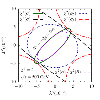
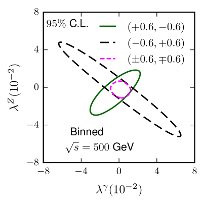
Figure 13: The $\chi^{2}=4$ contours of the unbinned cross section $\sigma=\sigma(+\eta_{3},+\xi_{3})$ in solid/green lines, $\bar{\sigma}=\sigma(-\eta_{3},-\xi_{3})$ in big-dashed/black lines, $\sigma_{T}=\sigma(+\eta_{3},+\xi_{3})+\sigma(-\eta_{3},-\xi_{3})$ in dotted/blue line, $\sigma_{A}=\sigma(+\eta_{3},+\xi_{3})-\sigma(-\eta_{3},-\xi_{3})$ in dash-dotted/red line and the combined $\chi^{2}$ of $\sigma$ and $\bar{\sigma}$ in dashed/magenta lines for polarization $(\eta_{3},\xi_{3})=(+0.6,-0.6)$ on $\lambda^{\gamma}$–$\lambda^{Z}$ plane are shown in the left-panel. The $95~{}\%$ C.L. contours from simultaneous analysis in $\lambda^{\gamma}$–$\lambda^{Z}$ plane for the beam polarization $(+0.6,-0.6)$, $(-0.6,+0.6)$ and their combined one $(\pm 0.6,\mp 0.6)$ are shown in the right-panel using all the binned observables, i.e., in the Binned case. The analyses are done for $\sqrt{s}=500$ GeV and ${\cal L}=50$ fb^-1 luminosity to each beam polarization set.

To reduce the systematic errors in analysis due to luminosity, the beam polarizations are flipped between two opposite choices frequently giving half the total luminosity to both the polarization choices in an $e^{+}$–$e^{-}$ collider. One can, in principle, use the observables, e.g., the total cross section ($\sigma_{T}$) or their difference ($\sigma_{A}$) as in Eqs. (7) & (8), respectively, or for the two opposite polarization choices ($\sigma$ & $\bar{\sigma}$) separately for a suitable analysis. In this work, we have combined the opposite beam polarization at the level of $\chi^{2}$ as given in Eq. (III.2) not at the level of observables as the former constrains the couplings better than any combinations and of-course the individuals. To depict this, we present the $\chi^{2}=4$ contours of the unbinned cross sections in Fig. 13 (left-panel) for beam polarization $(+0.6,-0.6)$ ($\sigma$) and $(-0.6,+0.6)$ ($\bar{\sigma}$) and the combinations $\sigma_{T}$ and $\sigma_{A}$ along with the combined $\chi^{2}$ in the $\lambda^{\gamma}$–$\lambda^{Z}$ plane for ${\cal L}=50$ fb^-1 luminosity to each polarization choice as representative. A systematic error of $2\%$ is used as a benchmark in the cross section. The nature of the contours can be explained as follows: In the $WW$ production, the aTGC contributions appear only in the $s$-channel (see Fig. 1), where initial state $e^{+}e^{-}$ couples through the $\gamma/Z$ boson and both left and right chiral electrons contribute almost equally. The $t$-channel diagram, however, is pure background and receives contribution only from left chiral electrons. As a result, the $\bar{\sigma}$ (big-dashed/black) contains more background than $\sigma$ (solid/green) leading to a weaker limit on the couplings. Further, inclusion of $\bar{\sigma}$ into $\sigma_{T}$ (dotted/blue) and $\sigma_{A}$ (dashed-dotted/red) reduces the signal to the background ratio, and hence they are less sensitive to the couplings. The total $\chi^{2}$ for the combined beam polarizations shown in dashed (magenta) is, of course, the best to constrain the couplings. This behaviour is reverified with the simultaneous analysis using the binned cross section and polarization asymmetries ($72$ observables in the Binned case) and shown in Fig. 13 (right-panel) in the same $\lambda^{\gamma}$–$\lambda^{Z}$ plane showing the $95~{}\%$ C.L. contours for beam polarizations $(+0.6,-0.6)$, $(-0.6,+0.6)$, and their combinations $(\pm 0.6,\mp 0.6)$. Thus, we choose to combine the opposite beam polarization choices at the level of $\chi^{2}$ rather than combining them at the level of observables.

References

- (1) CMS Collaboration, S. Chatrchyan et al., Observation of a new boson at a mass of 125 GeV with the CMS experiment at the LHC, Phys. Lett. B716 (2012) 30–61, arXiv:1207.7235 [hep-ex].
- (2) C. Bourrely, J. Soffer, and E. Leader, Polarization Phenomena in Hadronic Reactions, Phys. Rept. 59 (1980) 95–297.
- (3) OPAL Collaboration, G. Abbiendi et al., Measurement of boson polarizations and CP violating triple gauge couplings from production at LEP, Eur. Phys. J. C19 (2001) 229–240, arXiv:hep-ex/0009021 [hep-ex].
- (4) I. Ots, H. Uibo, H. Liivat, R. Saar, and R. K. Loide, Possible anomalous Z Z gamma and Z gamma gamma couplings and Z boson spin orientation in , Nucl. Phys. B702 (2004) 346–356.
- (5) F. Boudjema and R. K. Singh, A Model independent spin analysis of fundamental particles using azimuthal asymmetries, JHEP 07 (2009) 028, arXiv:0903.4705 [hep-ph].
- (6) J. A. Aguilar-Saavedra and J. Bernabeu, Breaking down the entire W boson spin observables from its decay, Phys. Rev. D93 no. 1, (2016) 011301, arXiv:1508.04592 [hep-ph].
- (7) R. Rahaman and R. K. Singh, On polarization parameters of spin-1 particles and anomalous couplings in , Eur. Phys. J. C76 no. 10, (2016) 539, arXiv:1604.06677 [hep-ph].
- (8) J. Nakamura, Polarisations of the and bosons in the processes and , JHEP 08 (2017) 008, arXiv:1706.01816 [hep-ph].
- (9) W. Buchmuller and D. Wyler, Effective Lagrangian Analysis of New Interactions and Flavor Conservation, Nucl. Phys. B268 (1986) 621–653.
- (10) K. Hagiwara, S. Ishihara, R. Szalapski, and D. Zeppenfeld, Low-energy effects of new interactions in the electroweak boson sector, Phys. Rev. D48 (1993) 2182–2203.
- (11) C. Degrande, N. Greiner, W. Kilian, O. Mattelaer, H. Mebane, T. Stelzer, S. Willenbrock, and C. Zhang, Effective Field Theory: A Modern Approach to Anomalous Couplings, Annals Phys. 335 (2013) 21–32, arXiv:1205.4231 [hep-ph].
- (12) Z. Zhang, Time to Go Beyond Triple-Gauge-Boson-Coupling Interpretation of Pair Production, Phys. Rev. Lett. 118 no. 1, (2017) 011803, arXiv:1610.01618 [hep-ph].
- (13) J. Baglio, S. Dawson, and S. Homiller, QCD corrections in Standard Model EFT fits to and production, Phys. Rev. D 100 no. 11, (2019) 113010, arXiv:1909.11576 [hep-ph].
- (14) K. Hagiwara, R. D. Peccei, D. Zeppenfeld, and K. Hikasa, Probing the Weak Boson Sector in , Nucl. Phys. B282 (1987) 253–307.
- (15) J. Wudka, Electroweak effective Lagrangians, Int. J. Mod. Phys. A9 (1994) 2301–2362, arXiv:hep-ph/9406205 [hep-ph].
- (16) K. J. F. Gaemers and G. J. Gounaris, Polarization Amplitudes for and , Z. Phys. C1 (1979) 259.
- (17) C. L. Bilchak and J. D. Stroughair, Pair Production in Colliders, Phys. Rev. D30 (1984) 1881.
- (18) K. Hagiwara, S. Ishihara, R. Szalapski, and D. Zeppenfeld, Low-energy constraints on electroweak three gauge boson couplings, Phys. Lett. B283 (1992) 353–359.
- (19) D. Choudhury and J. Kalinowski, Unraveling the and vertices at the linear collider: Anti-neutrino neutrino and anti-neutrino neutrino final states, Nucl. Phys. B491 (1997) 129–146, arXiv:hep-ph/9608416 [hep-ph].
- (20) D. Choudhury, J. Kalinowski, and A. Kulesza, CP violating anomalous couplings in collisions, Phys. Lett. B457 (1999) 193–201, arXiv:hep-ph/9904215 [hep-ph].
- (21) J. D. Wells and Z. Zhang, Status and prospects of precision analyses with , Phys. Rev. D93 no. 3, (2016) 034001, arXiv:1507.01594 [hep-ph]. [Phys. Rev.D93,034001(2016)].
- (22) G. Buchalla, O. Cata, R. Rahn, and M. Schlaffer, Effective Field Theory Analysis of New Physics in at a Linear Collider, Eur. Phys. J. C73 no. 10, (2013) 2589, arXiv:1302.6481 [hep-ph].
- (23) L. Berthier, M. Bjørn, and M. Trott, Incorporating doubly resonant data in a global fit of SMEFT parameters to lift flat directions, JHEP 09 (2016) 157, arXiv:1606.06693 [hep-ph].
- (24) L. Bian, J. Shu, and Y. Zhang, Prospects for Triple Gauge Coupling Measurements at Future Lepton Colliders and the 14 TeV LHC, JHEP 09 (2015) 206, arXiv:1507.02238 [hep-ph].
- (25) L. Bian, J. Shu, and Y. Zhang, Triple gauge couplings at future hadron and lepton colliders, Int. J. Mod. Phys. A31 no. 33, (2016) 1644008, arXiv:1612.03888 [hep-ph].
- (26) S. S. Biswal, M. Patra, and S. Raychaudhuri, Anomalous Triple Gauge Vertices at the Large Hadron-Electron Collider, arXiv:1405.6056 [hep-ph].
- (27) I. T. Cakir, O. Cakir, A. Senol, and A. T. Tasci, Search for anomalous and couplings with polarized -beam at the LHeC, Acta Phys. Polon. B45 no. 10, (2014) 1947, arXiv:1406.7696 [hep-ph].
- (28) R. Li, X.-M. Shen, K. Wang, T. Xu, L. Zhang, and G. Zhu, Probing anomalous triple gauge bosons coupling at the LHeC, Phys. Rev. D97 no. 7, (2018) 075043, arXiv:1711.05607 [hep-ph].
- (29) S. Kumar and P. Poulose, Probing coupling through at ILC, Int. J. Mod. Phys. A30 no. 36, (2015) 1550215, arXiv:1501.01380 [hep-ph].
- (30) U. Baur and D. Zeppenfeld, Unitarity Constraints on the Electroweak Three Vector Boson Vertices, Phys. Lett. B201 (1988) 383–389.
- (31) L. J. Dixon, Z. Kunszt, and A. Signer, Vector boson pair production in hadronic collisions at order : Lepton correlations and anomalous couplings, Phys. Rev. D60 (1999) 114037, arXiv:hep-ph/9907305 [hep-ph].
- (32) A. Falkowski, M. Gonzalez-Alonso, A. Greljo, D. Marzocca, and M. Son, Anomalous Triple Gauge Couplings in the Effective Field Theory Approach at the LHC, JHEP 02 (2017) 115, arXiv:1609.06312 [hep-ph].
- (33) A. Butter, O. J. P. Éboli, J. Gonzalez-Fraile, M. C. Gonzalez-Garcia, T. Plehn, and M. Rauch, The Gauge-Higgs Legacy of the LHC Run I, JHEP 07 (2016) 152, arXiv:1604.03105 [hep-ph].
- (34) A. Azatov, J. Elias-Miro, Y. Reyimuaji, and E. Venturini, Novel measurements of anomalous triple gauge couplings for the LHC, JHEP 10 (2017) 027, arXiv:1707.08060 [hep-ph].
- (35) J. Baglio, S. Dawson, and I. M. Lewis, An NLO QCD effective field theory analysis of production at the LHC including fermionic operators, Phys. Rev. D96 no. 7, (2017) 073003, arXiv:1708.03332 [hep-ph].
- (36) H. T. Li and G. Valencia, CP violating anomalous couplings in jet production at the LHC, Phys. Rev. D96 no. 7, (2017) 075014, arXiv:1708.04402 [hep-ph].
- (37) J. Baglio, S. Dawson, and I. M. Lewis, NLO effects in EFT fits to production at the LHC, Phys. Rev. D99 no. 3, (2019) 035029, arXiv:1812.00214 [hep-ph].
- (38) D. Bhatia, U. Maitra, and S. Raychaudhuri, Pinning down anomalous couplings at the LHC, Phys. Rev. D99 no. 9, (2019) 095017, arXiv:1804.05357 [hep-ph].
- (39) M. Chiesa, A. Denner, and J.-N. Lang, Anomalous triple-gauge-boson interactions in vector-boson pair production with RECOLA2, Eur. Phys. J. C78 no. 6, (2018) 467, arXiv:1804.01477 [hep-ph].
- (40) R. Rahaman and R. K. Singh, Unravelling the anomalous gauge boson couplings in production at the LHC and the role of spin- polarizations, JHEP 04 (2020) 075, arXiv:1911.03111 [hep-ph].
- (41) A. Azatov, D. Barducci, and E. Venturini, Precision diboson measurements at hadron colliders, JHEP 04 (2019) 075, arXiv:1901.04821 [hep-ph].
- (42) OPAL Collaboration, G. Abbiendi et al., Measurement of charged current triple gauge boson couplings using pairs at LEP, Eur. Phys. J. C33 (2004) 463–476, arXiv:hep-ex/0308067 [hep-ex].
- (43) DELPHI Collaboration, J. Abdallah et al., Study of W boson polarisations and Triple Gauge boson Couplings in the reaction at LEP 2, Eur. Phys. J. C54 (2008) 345–364, arXiv:0801.1235 [hep-ex].
- (44) DELPHI, OPAL, LEP Electroweak, ALEPH, L3 Collaboration, S. Schael et al., Electroweak Measurements in Electron-Positron Collisions at W-Boson-Pair Energies at LEP, Phys. Rept. 532 (2013) 119–244, arXiv:1302.3415 [hep-ex].
- (45) CDF Collaboration, T. Aaltonen et al., Limits on Anomalous Triple Gauge Couplings in Collisions at = 1.96 TeV, Phys. Rev. D76 (2007) 111103, arXiv:0705.2247 [hep-ex].
- (46) D0 Collaboration, V. M. Abazov et al., Limits on anomalous trilinear gauge boson couplings from , and production in collisions at TeV, Phys. Lett. B718 (2012) 451–459, arXiv:1208.5458 [hep-ex].
- (47) CMS Collaboration, V. Khachatryan et al., Measurement of the WZ production cross section in pp collisions at and 8 TeV and search for anomalous triple gauge couplings at , Eur. Phys. J. C77 no. 4, (2017) 236, arXiv:1609.05721 [hep-ex].
- (48) ATLAS Collaboration, G. Aad et al., Measurements of production cross sections in collisions at TeV with the ATLAS detector and limits on anomalous gauge boson self-couplings, Phys. Rev. D93 no. 9, (2016) 092004, arXiv:1603.02151 [hep-ex].
- (49) ATLAS Collaboration, G. Aad et al., Measurement of total and differential production cross sections in proton-proton collisions at TeV with the ATLAS detector and limits on anomalous triple-gauge-boson couplings, JHEP 09 (2016) 029, arXiv:1603.01702 [hep-ex].
- (50) CMS Collaboration, S. Chatrchyan et al., Measurement of the Cross section in Collisions at TeV and Limits on Anomalous and couplings, Eur. Phys. J. C73 no. 10, (2013) 2610, arXiv:1306.1126 [hep-ex].
- (51) CMS Collaboration, P. Rebello Teles, Search for anomalous gauge couplings in semi-leptonic decays of and in pp collisions at 8 TeV, in Meeting of the APS Division of Particles and Fields (DPF 2013) Santa Cruz, California, USA, August 13-17, 2013. 2013. arXiv:1310.0473 [hep-ex]. https://inspirehep.net/record/1256468/files/arXiv:1310.0473.pdf.
- (52) ATLAS Collaboration, G. Aad et al., Measurement of production in pp collisions at TeV with the ATLAS detector and limits on anomalous and couplings, Phys. Rev. D87 no. 11, (2013) 112001, arXiv:1210.2979 [hep-ex]. [Erratum: Phys. Rev.D88,no.7,079906(2013)].
- (53) CMS Collaboration, S. Chatrchyan et al., Measurement of the sum of and production with dijet events in collisions at TeV, Eur. Phys. J. C73 no. 2, (2013) 2283, arXiv:1210.7544 [hep-ex].
- (54) ATLAS Collaboration, G. Aad et al., Measurements of and production in collisions at =7 TeV with the ATLAS detector at the LHC, Phys. Rev. D87 no. 11, (2013) 112003, arXiv:1302.1283 [hep-ex]. [Erratum: Phys. Rev.D91,no.11,119901(2015)].
- (55) CMS Collaboration, S. Chatrchyan et al., Measurement of the and inclusive cross sections in collisions at TeV and limits on anomalous triple gauge boson couplings, Phys. Rev. D89 no. 9, (2014) 092005, arXiv:1308.6832 [hep-ex].
- (56) ATLAS Collaboration, M. Aaboud et al., Measurement of production with the hadronically decaying boson reconstructed as one or two jets in collisions at TeV with ATLAS, and constraints on anomalous gauge couplings, Eur. Phys. J. C77 no. 8, (2017) 563, arXiv:1706.01702 [hep-ex].
- (57) CMS Collaboration, A. M. Sirunyan et al., Search for anomalous couplings in boosted production in proton-proton collisions at 8 TeV, Phys. Lett. B772 (2017) 21–42, arXiv:1703.06095 [hep-ex].
- (58) ATLAS Collaboration, M. Aaboud et al., Measurements of electroweak production and constraints on anomalous gauge couplings with the ATLAS detector, Eur. Phys. J. C77 no. 7, (2017) 474, arXiv:1703.04362 [hep-ex].
- (59) CMS Collaboration, A. M. Sirunyan et al., Electroweak production of two jets in association with a Z boson in proton–proton collisions at 13 TeV, Eur. Phys. J. C78 no. 7, (2018) 589, arXiv:1712.09814 [hep-ex].
- (60) CMS Collaboration, A. M. Sirunyan et al., Search for anomalous triple gauge couplings in WW and WZ production in lepton + jet events in proton-proton collisions at 13 TeV, JHEP 12 (2019) 062, arXiv:1907.08354 [hep-ex].
- (61) CMS Collaboration, A. M. Sirunyan et al., Measurement of electroweak production of a boson in association with two jets in proton–proton collisions at , Eur. Phys. J. C 80 no. 1, (2020) 43, arXiv:1903.04040 [hep-ex].
- (62) CMS Collaboration, A. M. Sirunyan et al., Measurements of the pp WZ inclusive and differential production cross section and constraints on charged anomalous triple gauge couplings at 13 TeV, JHEP 04 (2019) 122, arXiv:1901.03428 [hep-ex].
- (63) T. Corbett, O. J. P. Éboli, J. Gonzalez-Fraile, and M. C. Gonzalez-Garcia, Determining Triple Gauge Boson Couplings from Higgs Data, Phys. Rev. Lett. 111 (2013) 011801, arXiv:1304.1151 [hep-ph].
- (64) ILC Collaboration, G. Aarons et al., International Linear Collider Reference Design Report Volume 2: Physics at the ILC, arXiv:0709.1893 [hep-ph].
- (65) H. Baer, T. Barklow, K. Fujii, Y. Gao, A. Hoang, S. Kanemura, J. List, H. E. Logan, A. Nomerotski, M. Perelstein, et al., The International Linear Collider Technical Design Report - Volume 2: Physics, arXiv:1306.6352 [hep-ph].
- (66) T. Behnke, J. E. Brau, B. Foster, J. Fuster, M. Harrison, J. M. Paterson, M. Peskin, M. Stanitzki, N. Walker, and H. Yamamoto, The International Linear Collider Technical Design Report - Volume 1: Executive Summary, arXiv:1306.6327 [physics.acc-ph].
- (67) G. Moortgat-Pick et al., The Role of polarized positrons and electrons in revealing fundamental interactions at the linear collider, Phys. Rept. 460 (2008) 131–243, arXiv:hep-ph/0507011 [hep-ph].
- (68) G. Gounaris, J. Layssac, G. Moultaka, and F. M. Renard, Analytic expressions of cross-sections, asymmetries and W density matrices for with general three boson couplings, Int. J. Mod. Phys. A8 (1993) 3285–3320.
- (69) B. Ananthanarayan, M. Patra, and P. Poulose, W physics at the ILC with polarized beams as a probe of the Littlest Higgs Model, JHEP 11 (2009) 058, arXiv:0909.5323 [hep-ph].
- (70) B. Ananthanarayan, M. Patra, and P. Poulose, Signals of additional Z boson in at the ILC with polarized beams, JHEP 02 (2011) 043, arXiv:1012.3566 [hep-ph].
- (71) B. Ananthanarayan, M. Patra, and P. Poulose, Probing strongly interacting W’s at the ILC with polarized beams, JHEP 03 (2012) 060, arXiv:1112.5020 [hep-ph].
- (72) V. V. Andreev, G. Moortgat-Pick, P. Osland, A. A. Pankov, and N. Paver, Discriminating Z’ from Anomalous Trilinear Gauge Coupling Signatures in at ILC with Polarized Beams, Eur. Phys. J. C72 (2012) 2147, arXiv:1205.0866 [hep-ph].
- (73) J. A. Aguilar-Saavedra, J. Bernabéu, V. A. Mitsou, and A. Segarra, The Z boson spin observables as messengers of new physics, Eur. Phys. J. C77 no. 4, (2017) 234, arXiv:1701.03115 [hep-ph].
- (74) F. M. Renard, Polarization effects due to dark matter interaction between massive standard particles, arXiv:1802.10313 [hep-ph].
- (75) F. M. Renard, Z Polarization in for testing the top quark mass structure and the presence of final interactions, arXiv:1803.10466 [hep-ph].
- (76) F. M. Renard, W polarization in , gluon-gluon and for testing the top quark mass structure and the presence of final interactions, arXiv:1807.00621 [hep-ph].
- (77) F. M. Renard, Further tests of special interactions of massive particles from the Z polarization rate in and in , arXiv:1808.05429 [hep-ph].
- (78) F. M. Renard, Z polarization in for testing special interactions of massive particles, arXiv:1807.08938 [hep-ph].
- (79) S. Behera, R. Islam, M. Kumar, P. Poulose, and R. Rahaman, Fingerprinting the Top quark FCNC via anomalous couplings at the LHeC, Phys. Rev. D100 no. 1, (2019) 015006, arXiv:1811.04681 [hep-ph].
- (80) R. Rahaman and R. K. Singh, On the choice of beam polarization in and anomalous triple gauge-boson couplings, Eur. Phys. J. C77 no. 8, (2017) 521, arXiv:1703.06437 [hep-ph].
- (81) R. Rahaman and R. K. Singh, Anomalous triple gauge boson couplings in production at the LHC and the role of boson polarizations, Nucl. Phys. B948 (2019) 114754, arXiv:1810.11657 [hep-ph].
- (82) ATLAS Collaboration, M. Aaboud et al., Measurement of production cross sections and gauge boson polarisation in collisions at TeV with the ATLAS detector, Eur. Phys. J. C79 no. 6, (2019) 535, arXiv:1902.05759 [hep-ex].
- (83) A. A. Pankov, N. Paver, and A. V. Tsytrinov, Distinguishing new physics scenarios at a linear collider with polarized beams, Phys. Rev. D73 (2006) 115005, arXiv:hep-ph/0512131 [hep-ph].
- (84) P. Osland, A. A. Pankov, and A. V. Tsytrinov, Identification of extra neutral gauge bosons at the International Linear Collider, Eur. Phys. J. C67 (2010) 191–204, arXiv:0912.2806 [hep-ph].
- (85) D. Choudhury and S. D. Rindani, Test of CP violating neutral gauge boson vertices in , Phys. Lett. B335 (1994) 198–204, arXiv:hep-ph/9405242 [hep-ph].
- (86) H. Czyz, K. Kolodziej, and M. Zralek, Composite Boson and CP Violation in the Process , Z. Phys. C43 (1989) 97.
- (87) B. Ananthanarayan and S. D. Rindani, CP violation at a linear collider with transverse polarization, Phys. Rev. D70 (2004) 036005, arXiv:hep-ph/0309260 [hep-ph].
- (88) B. Ananthanarayan, S. D. Rindani, R. K. Singh, and A. Bartl, Transverse beam polarization and CP-violating triple-gauge-boson couplings in , Phys. Lett. B593 (2004) 95–104, arXiv:hep-ph/0404106 [hep-ph]. [Erratum: Phys. Lett.B608,274(2005)].
- (89) A. Bartl, H. Fraas, S. Hesselbach, K. Hohenwarter-Sodek, T. Kernreiter, and G. A. Moortgat-Pick, CP-odd observables in neutralino production with transverse e+ and e- beam polarization, JHEP 01 (2006) 170, arXiv:hep-ph/0510029 [hep-ph].
- (90) K. Rao and S. D. Rindani, Probing CP-violating contact interactions in with polarized beams, Phys. Lett. B642 (2006) 85–92, arXiv:hep-ph/0605298 [hep-ph].
- (91) A. Bartl, K. Hohenwarter-Sodek, T. Kernreiter, and O. Kittel, CP asymmetries with longitudinal and transverse beam polarizations in neutralino production and decay into the Z0 boson at the ILC, JHEP 09 (2007) 079, arXiv:0706.3822 [hep-ph].
- (92) H. K. Dreiner, O. Kittel, and A. Marold, Normal tau polarisation as a sensitive probe of CP violation in chargino decay, Phys. Rev. D82 (2010) 116005, arXiv:1001.4714 [hep-ph].
- (93) O. Kittel, G. Moortgat-Pick, K. Rolbiecki, P. Schade, and M. Terwort, Measurement of CP asymmetries in neutralino production at the ILC, Eur. Phys. J. C72 (2012) 1854, arXiv:1108.3220 [hep-ph].
- (94) B. Ananthanarayan, S. K. Garg, M. Patra, and S. D. Rindani, Isolating CP-violating ZZ coupling in Z with transverse beam polarizations, Phys. Rev. D85 (2012) 034006, arXiv:1104.3645 [hep-ph].
- (95) J. Alwall, R. Frederix, S. Frixione, V. Hirschi, F. Maltoni, O. Mattelaer, H. S. Shao, T. Stelzer, P. Torrielli, and M. Zaro, The automated computation of tree-level and next-to-leading order differential cross sections, and their matching to parton shower simulations, JHEP 07 (2014) 079, arXiv:1405.0301 [hep-ph].
- (96) A. Alloul, N. D. Christensen, C. Degrande, C. Duhr, and B. Fuks, FeynRules 2.0 - A complete toolbox for tree-level phenomenology, Comput. Phys. Commun. 185 (2014) 2250–2300, arXiv:1310.1921 [hep-ph].
- (97) A. Vauth and J. List, Beam Polarization at the ILC: Physics Case and Realization, Int. J. Mod. Phys. Conf. Ser. 40 (2016) 1660003.
- (98) G. Moortgat-Pick, Physics aspects of polarized e+ at the linear collider, in 1st International Positron Source Workshop (POSIPOL 2006) Geneva, Switzerland, April 26-28, 2006. 2006. arXiv:hep-ph/0607173 [hep-ph]. http://weblib.cern.ch/abstract?CERN-PH-TH-2006-128.
- (99) T. Barklow, J. Brau, K. Fujii, J. Gao, J. List, N. Walker, and K. Yokoya, ILC Operating Scenarios, arXiv:1506.07830 [hep-ex].
- (100) P. Bambade et al., The International Linear Collider: A Global Project, arXiv:1903.01629 [hep-ex].