A new Monte Carlo-based fitting method

Abstract

We present a new fitting technique based on the parametric bootstrap method, which relies on the idea to produce artificial measurements using the estimated probability distribution of the experimental data. In order to investigate the main properties of this technique, we develop a toy model and we analyze several fitting conditions with a comparison of our results to the ones obtained using both the standard $\chi^{2}$ minimization procedure and a Bayesian approach. Furthermore, we investigate the effect of the data systematic uncertainties both on the probability distribution of the fit parameters and on the shape of the expected goodness-of-fit distribution. Our conclusion is that, when systematic uncertainties are included in the analysis, only the bootstrap procedure is able to provide reliable confidence intervals and $p$-values, thus improving the results given by the standard $\chi^{2}$ minimization approach. Our technique is then applied to an actual physics process, the real Compton scattering off the proton, thus confirming both the portability and the validity of the bootstrap-based fit method.

I A brief summary of a best-fit procedure

The main goal of a best-fit procedure is the estimate of some unknown parameters, which a given model depends on. The more commonly used algorithm is the so-called least squares method, which is based on the function:

$$\chi_{stand}^{2}(\bm{\theta})=\sum_{i}{\left(\frac{E_{i}-T_{i}(\bm{\theta})}{\sigma_{i}}\right)^{2}}\ ,$$ (1)

where $E_{i}$ are the experimental values, $\sigma_{i}$ are their corresponding statistical uncertainties in root mean square (rms) units and $T_{i}$ are given by a theoretical model depending on the set of unknown parameters $\bm{\theta}$ to be evaluated from the data. The optimal parameter set $\hat{\bm{\theta}}$ is the one that minimizes $\chi_{stand}^{2}$ and this solution can be written as:

$$\chi_{min}^{2}=\sum_{i}{\left(\frac{E_{i}-T_{i}(\hat{\bm{\theta}})}{\sigma_{i}}\right)^{2}}.$$ (2)

Even though this procedure is commonly used in several scientific domains, its practical implementation often presents problems. One of them is the inclusion of the systematic uncertainties associated to the experimental data. If we consider the very simple case of a scaling factor parameter common to all data, the usual way to proceed is to modify Eq. (1) as follows (see, for instance, D’Agostini (1994)):

$$\chi_{mod}^{2}(\bm{\theta},f)=\sum_{i}{\left(\frac{fE_{i}-T_{i}(\bm{\theta})}{f\sigma_{i}}\right)^{2}}+\left(\frac{f-1}{\sigma_{sys}}\right)^{2}.$$ (3)

Here $f$ is a normalization factor to be treated as an additional fit parameter and $\sigma_{sys}$ is its estimated uncertainty (in rms units). However this equation is strictly valid only in the case of Gaussian systematic uncertainties, since

$$\chi_{mod}^{2}(\bm{\theta},f)=-2\ln{\mathcal{L}(\bm{\theta},f)}\ ,$$ (4)

where the Likelihood function $\mathcal{L}(\bm{\theta},f)$ is the product of the normal distributions with mean and standard deviations given by the experimental data multiplied by the normal distribution modeling the common systematic scale uncertainty, i.e. :

$$\mathcal{L}(\bm{\theta},f)=\prod_{i}\left[\frac{1}{\sigma^{2}_{i}\sqrt{2\pi}}e^{-\frac{(fE_{i}-T_{i}(\bm{\theta}))^{2}}{2f\sigma^{2}_{i}}}\right]\cdot\frac{1}{\sigma^{2}_{sys}\sqrt{2\pi}}e^{-\frac{(f-1)^{2}}{2\sigma^{2}_{sys}}}.$$ (5)

Moreover, especially with a large data base, this solution becomes unpractical since a different normalization parameter is needed for each subset and $\sigma_{sys}$ may as well change from point to point. Furthermore, when non-Gaussian and/or correlated uncertainties are present, as in the previous case, the $\chi_{min}^{2}$ value does not generally follow the standard $\chi^{2}$-distribution, since it is not a sum of squared, indepedendent, standard Gaussian random variables. The evaluation of the goodness of fit then becomes quite difficult, since the $\chi^{2}$ test cannot be used.

The model $T$ may also not only depend on the parameter set $\bm{\theta}$, but also on some additional, non-fitted (nuisance) parameters $\bm{\psi}$ evaluated from experimental data, that can be written under the form:

$$\bm{\psi}=\bar{\bm{\psi}}_{f}\pm\bm{\sigma}_{\psi}.$$ (6)

Here, $\bar{\bm{\psi}}$ and $\bm{\sigma}_{\psi}$ are their estimated values and uncertainties (in rms units), respectively. In this case, another critical feature is to evaluate the effect of $\bm{\sigma}_{\psi}$ on the final fit results. The total uncertainty on the fit parameters should be written as the sum of the pure contribution coming from the minimization itself and the uncertainty related to the effect of $\bm{\sigma_{\psi}}$ on the fit parameters. This last contribution can be evaluated according to the (linearly approximated) uncertainty propagation as

$$\delta\hat{\bm{\theta}}_{extra,ab}\simeq\sum_{cd}\left(\left.\frac{\partial\bm{\theta}_{a}}{\partial\bm{\psi}_{c}}\right|_{\bm{\theta}_{a}=\hat{\bm{\theta}}_{a}}\right)\sigma_{\psi,cd}\left(\left.\frac{\partial\bm{\theta}_{b}}{\partial\bm{\psi}_{d}}\right|_{\bm{\theta}_{b}=\hat{\bm{\theta}}_{b}}\right),$$ (7)

where the indexes $a,b$ run over the components of $\bm{\theta}$, while $c,d$ on the components of $\bm{\psi}$. The quantity $\delta\hat{\bm{\theta}}_{extra,ab}$ thus includes both the covariances and the variances, obtained when $a\equiv b$. Furthermore, the terms in round brackets can be evaluated as

$$\left.\frac{\partial\bm{\theta}_{x}}{\partial\bm{\psi}_{y}}\right|_{\bm{\theta}_{x}=\hat{\bm{\theta}}_{x}}=\left[\left(\frac{\partial T}{\partial\bm{\theta}_{x}}\right)^{-1}\frac{\partial T}{\partial\bm{\psi}_{y}}\right]_{\bm{\theta}_{x}=\hat{\bm{\theta}}_{x}}.$$ (8)

However, if the analytical structure of the model is complicated, the term $(\partial T)/(\partial\bm{\psi}_{y})$ could be hard to be obtained, even numerically, thus requiring the application of a different strategy.

Our new method is able to solve all these problems in a straightforward way and, even if we apply it within the least squares framework, it can, in principle, also be used with other minimization schemes, as the Maximum Likelihood (ML) approach.

The manuscript is organized as follows. In Sec. II we give a general outline of our new method and we describe in detail its more relevant features by considering a general example of a fit of data with both statistical and systematic uncertainties. In Section III and Section IV we perform an accurate check of the new method using two different toy models and simulated data. The results thus obtained under different fit conditions are also compared both to the ones coming form the standard $\chi^{2}$ fit procedure and to the ones obtained using, as an alternative approach, the Hierarchical Bayesian Model (HBM) described in de Souza et al. (2019).

In Sec. V we apply our method to an actual physics process, the real Compton scattering off the proton. Here we briefly summarize the results that have already been published (see Ref. Pasquini et al. (2019)) and complement them with additional information by giving an estimated of the experimental biases of the fitted data and by evaluating the expected goodness-of-fit distribution both with the exclusion and the inclusion of the systematic uncertainties in the fit procedure. Finally, our conclusions are drawn in Sec. VI.

II Outline of the new method

Our new method is based on the parametric bootstrap technique (see, for instance, Davidson and Hinkley (1997) and references therein). It requires, for each point $E_{i}$, measured at a given set of known parameters $\bm{x}$, the knowledge of the probability density function $p({\bm{x}})$ of its evaluated uncertainty. The core idea is to assume each single $E_{i}$ to be the ML estimate of its true and unknown value $\mathcal{E}_{i}$. In this case, the density $p({\bm{x}},E_{i})$ is taken as an approximation of the true density $p({\bm{x}},{\mathcal{E}_{i}})$:

$$p({\bm{x}},\mathcal{E}_{i})\simeq p(\bm{x},E_{i}).$$ (9)

Then a random bootstrap sample $E^{b}_{1},E^{b}_{2}\ldots E^{b}_{n}$ is generated, for each $E_{i}$, according to $p(x,E_{i})$. Using this sample, an estimate of the true model parameters $\bm{\theta}^{b}$ is obtained using the standard minimization tools (simplex, gradient, …) applied to the function given in Eq. (1).

Repeating this bootstrap cycle a (very) large number $n_{b}$ of times, we get a sample $\hat{\bm{\theta}}^{b}_{1},\hat{\bm{\theta}}^{b}_{2}\ldots\hat{\bm{\theta}}^{b}_{n_{b}}$ from which we are finally able to reconstruct the true probability distributions for every fit parameter. For instance, the sample mean and the sample standard deviation are given as:

$$\hat{\bm{\theta}}^{b}=\frac{1}{n_{b}}\sum^{n_{b}}_{i=1}{\hat{\bm{\theta}}^{b}_{i}}\quad,\quad\sigma_{\hat{\bm{\theta}}^{b}}=\left[\frac{1}{n_{b}-1}\sum_{i=1}^{n_{b}}\left(\hat{\bm{\theta}}_{i}^{b}-\hat{\bm{\theta}}^{b}\right)^{2}\right]^{1/2}.$$ (10)

II.1 A general example

As a general example, we consider the case of a database composed by different and independent subsets and with a total of $n$ experimental points having both statistical and systematic uncertainties independent of each other. The best estimate of the true value $\mathcal{E}_{i}$ of each experimental point can then be written as:

$$E_{i}\pm\sigma_{i}^{\text{stat}}\pm\sigma_{i}^{\text{sys}}\ ,$$ (11)

where $\sigma_{i}^{\text{stat}}$ and $\sigma_{i}^{\text{sys}}$ are the standard deviations of the statistical and systematic uncertainties, respectively.

Now we suppose to have Gaussian-distributed statistical uncertaintes and, to be in the same conditions as in Eq. (3), we also assume that all the points of each subset have the same scaling factor uncertainty $\Delta$. This parameter is different for each subset and represents the half width of a uniform distribution. In the first step of our procedure, each artificial bootstrap “measurement” is assumed to be Gaussian distributed around a given experimental data point with a standard deviation given by its statistical uncertainty (see Eq. (11)). Then, all bootstrapped points of a given subset are shifted by the same random quantity uniformly distributed within the estimated systematic uncertainty interval.

If we define a cycle as when the number of bootstrapped points are equal to the total number of points in the considered experimental set, the bootstrap sampling can be finally described for each subset $k$ as:

$$\mathcal{B}_{lj}=(1+\delta_{k,j})(E_{i}+\gamma_{lj}\sigma_{m})\quad\forall k=1,\ldots,n_{s},$$ (12)

where $\mathcal{B}_{lj}$ is a generic bootstrapped point with the index $l$ running over the number of data points in each subset ($n_{k}$) and the index $j$ indicates the $j^{th}$ bootstrap cycle. The $\gamma_{lj}$ parameters are sampled from the standard Gaussian distribution $\mathcal{N}[0,1]$, while the $\delta_{k,j}$ are random numbers uniformly distributed as $\mathcal{U}[-\Delta_{k},+\Delta_{k}]$, being $\pm\Delta_{k}$ the percentage systematic uncertainty of each subset $k$ ($k$ runs from 1 to the number of the different data subsets $n_{s}$). If only statistical uncertainties have been taken into account, the systematic sources can be easily excluded from this procedure by just imposing $\delta_{k,j}\equiv 0\ \ \forall k=1,\ldots,n_{s}$.

After a complete cycle and once defined:

$$\delta_{lj} \equiv \delta_{k,j}\quad\forall l\in\text{ set k}\quad;\quad\forall k=1,\ldots,n_{s}\ ,$$

$$\sigma_{lj} \equiv (1+\delta_{lj})\sigma_{l}\ ,$$ (13)

the minimization procedure is performed on the function:

$$\chi_{j}^{2}=\sum^{n}_{i=1}{\left(\frac{\mathcal{B}_{ij}-T_{i}(\bm{\theta})}{\sigma_{ij}}\right)^{2}},$$ (14)

with the index $i$ running over the total number of data points $n$, and all the fit results are stored.

The main advantages of the adopted technique are:

• the straightforward inclusion of systematic uncertainties in the minimization procedure, as shown in Eq. (12). This feature allows us to reduce the overall number of fit parameters with respect to the modified $\chi^{2}$ procedure, where a normalization factor for each data set is left as free parameters (see Eq. (3));

• any kind of uncertainty distribution of the experimental data can be easily implemented;

• the probability distributions of the fit parameters are not assumed a priori, but are directly evaluated from the distributions assigned to the experimental data;

• the uncertainty on the fit parameters can be estimated also when the used mathematical minimization algorithm does not provide them as, for example, in the case of the simplex method.

When additional model parameters $\bm{\psi}$ are present (see Eq. (6)) and their probability distribution $g(\bm{\psi},\bm{\sigma}_{\psi})$ is known, their uncertainties can be easily included in this algorithm by sampling at every cycle an additional random variable $\bm{\psi}_{j}$ distributed as $g(\bm{\psi},\bm{\sigma}_{\psi})$. The minimization function of Eq. (14) is accordingly generalized as:

$$\chi_{b,j}^{2}=\sum_{i=1}^{n}\left(\frac{\mathcal{B}_{ij}-T_{i}(\bm{\psi}_{j},\bm{\theta})}{\sigma_{ij}}\right)^{2},$$ (15)

and its minimum value can be written as:

$${\hat{\chi}^{2}_{b,j}}=\sum_{i=1}^{n}\left(\frac{\mathcal{B}_{ij}-T_{i}(\bm{\psi}_{j},\hat{\bm{\theta}}_{j})}{\sigma_{ij}}\right)^{2}.$$ (16)

II.2 The meaning of $\hat{\chi}_{b,j}^{2}$ in parametric bootstrap

The value of ${\hat{\chi}^{2}_{b,j}}$ given in Eq. (16) cannot be treated as the standard $\hat{\chi}^{2}$ value commonly used to assess the goodness of a fit in the standard procedure, i.e.

$$\hat{\chi}^{2}=\sum_{i=1}^{n}\left(\frac{E_{i}-T_{i}(\bm{\psi},\hat{\bm{\theta}})}{\sigma_{i}}\right)^{2},$$ (17)

due to the artificial statistical fluctuations inherent to each bootstrapped sampling.

In the following, we will find the connection between ${\hat{\chi}^{2}_{b,j}}$ and $\hat{\chi}^{2}$. After introducing the following definitions,

$$\epsilon_{ij} \equiv \frac{1}{\sigma_{i}}\left[T_{i}(\bm{\psi},\hat{\bm{\theta}})-\frac{T_{i}(\bm{\psi},\hat{\bm{\theta}}_{j})}{1+\delta_{ij}}\right],$$

$$\eta_{ij} \equiv \frac{1}{(1+\delta_{ij})\sigma_{i}}\left[T_{i}(\bm{\psi},\hat{\bm{\theta}}_{j})-T_{i}(\bm{\psi}_{j},\hat{\bm{\theta}}_{j})\right],$$ (18)

we can rewrite the $T_{i}(\bm{\psi}_{j},\hat{\bm{\theta}}_{j})$ term of Eq. (16) as

$$T_{i}(\bm{\psi}_{j},\hat{\bm{\theta}}_{j})=(1+\delta_{ij})\left[T_{i}(\bm{\psi},\hat{\bm{\theta}})-\sigma_{i}(\epsilon_{ij}+\eta_{ij})\right].$$ (19)

The $\epsilon_{ij}$ parameter, once summed over $i$, quantifies the difference between the model evaluated at the global best values of the fitting parameters $\hat{\bm{\theta}}$ and the model evaluated at the $j^{th}$ best values of $\bm{\theta}$ (i.e. $\hat{\bm{\theta}}_{j}$), taking into account both the statistical and systematic uncertainties. The $\eta_{ij}$ term is related to the effect that the uncertainties on the additional parameter set $\bm{\psi}$ have on the model evaluation of the generic observable $E_{i}$. Thanks to the previous formalism, we can rewrite Eq. (16) as

$${\hat{\chi}^{2}_{b,j}}=\hat{\chi}^{2}+\sum_{i}\gamma_{ij}^{2}+\sum_{i}\epsilon_{ij}^{2}+\sum_{i}D_{ij}+\sum_{i}\Phi_{ij},$$ (20)

where:

$$D_{ij} \equiv 2\left[\epsilon_{ij}\gamma_{ij}+\frac{1}{\sigma_{i}}(\epsilon_{ij}+\gamma_{ij})(E_{i}-T_{i}(\bm{\psi},\hat{\bm{\theta}}))\right],$$

$$\Phi_{ij} \equiv \eta_{ij}^{2}+2\eta_{ij}\left[(\epsilon_{ij}+\gamma_{ij})+\frac{1}{\sigma_{i}}(E_{i}-T_{i}(\bm{\psi},\hat{\bm{\theta}}))\right].$$ (21)

Thanks to the decomposition given in Eq. (20), from the ${\hat{\chi}^{2}_{b,j}}$ parameter we can isolate and identify: (i) the pure squared Gaussian term ($\sum_{i}\gamma_{ij}^{2}$); (ii) the main contribution related to the difference between the best evaluation of the model parameters obtained at the end of each bootstrap cycle and at the end of the full procedure ($\sum_{i}\epsilon_{ij}^{2}$); (iii) the term containing the effect of the error due to the uncertainties on the additional model parameters ($\sum_{i}\Phi_{ij}$); and (iv) a parameter with the mixed contributions due to the non-quadratic and $\eta$-independent terms ($\sum_{i}D_{ij}$).

Inverting the decomposition of Eq. (20), we can get the evaluation of $\hat{\chi}^{2}$ in the bootstrap framework. Within the small numerical approximations introduced by the Monte-Carlo procedure, after each bootstrap cycle such a value has to be identical to the one that can be directly computed from Eq. (17) at the very end of the bootstrap procedure. This cross-check is crucial for the auto-consistency of the fitting method: if $\hat{\chi}^{2}\neq{\hat{\chi}^{2}_{b,j}}-\left(\sum_{i}\gamma_{ij}^{2}+\sum_{i}\epsilon_{ij}^{2}+\sum_{i}D_{ij}+\sum_{i}\Phi_{ij}\right)$, there could be some mistakes in the sampling scheme or in the minimization procedure.

II.3 Evaluation of the expected goodness-of-fit distribution

Once the analytical form of the minimization function and the decomposition of its minimum value have been established, it is still necessary to determine a goodness-of-fit distribution, from which the associated $p$-value have to be computed. This procedure is detailed below.

Within this framework, the expected distribution can be evaluated assuming the model $T_{i}(\bm{\psi},\hat{\bm{\theta}})$ to be correct and by considering an ideal situation in which the experimental points are exactly the values predicted by our model.

The sampling procedure outlined above (see Eq. (12)) can then be repeated replacing each experimental data with $T_{i}(\bm{\psi},\hat{\bm{\theta}})$. We thus obtain:

$$\mathcal{M}_{ij}=(1+\delta_{ij})(T_{i}(\bm{\psi},\hat{\bm{\theta}})+\gamma_{ij}\sigma_{i}).$$ (22)

The minimization function can then be defined as:

$$\chi_{th,j}^{2}=\sum_{i=1}^{n}\left(\frac{\mathcal{M}_{ij}-T_{i}(\bm{\psi}_{j},\bm{\theta})}{\sigma_{ij}}\right)^{2},$$ (23)

and we denote its minimum value after the $j$-th cycle as:

$${\hat{\chi}^{2}_{th,j}}=\sum_{i=1}^{n}\left(\frac{\mathcal{M}_{ij}-T_{i}(\bm{\psi}_{j},\hat{\bm{\theta}}_{j}^{\prime})}{\sigma_{ij}}\right)^{2}.$$ (24)

The sampled parameters $\bm{\psi}_{j}$ are exactly the same as in Eq. (15), while the fit values of the parameters at every bootstrap cycle are, in general, different from the ones obtained from the fit of the bootstrapped data: for this reason we use the symbol $\hat{\bm{\theta}}_{j}^{\prime}$ instead of $\hat{\bm{\theta}}_{j}$. According to this notation, we can apply the same decomposition as before, thus defining

$$\epsilon_{ij}^{\prime} \equiv \frac{1}{\sigma_{i}}\left[T_{i}(\bm{\psi},\hat{\bm{\theta}})-\frac{T_{i}(\bm{\psi},\hat{\bm{\theta}}_{j}^{\prime})}{1+\delta_{ij}}\right],$$

$$\eta_{ij}^{\prime} \equiv \frac{1}{(1+\delta_{ij})\sigma_{i}}\left[T_{i}(\bm{\psi},\hat{\bm{\theta}}_{j}^{\prime})-T_{i}(\bm{\psi}_{j},\hat{\bm{\theta}}_{j}^{\prime})\right],$$

$$D_{ij}^{\prime} \equiv 2\epsilon_{ij}^{\prime}\gamma_{ij},$$

$$\Phi_{ij}^{\prime} \equiv {\eta_{ij}^{\prime}}^{2}+2\eta_{ij}^{\prime}\left(\epsilon_{ij}^{\prime}+\gamma_{ij}\right).$$ (25)

The resulting decomposition for ${\hat{\chi}^{2}_{th,j}}$ is

$${{\hat{\chi}}^{2}_{th,j}}=\hat{\chi}_{th}^{2}+\sum_{i}\gamma_{ij}^{2}+\sum_{i}{\epsilon_{ij}^{\prime}}^{2}+\sum_{i}D_{ij}^{\prime}+\sum_{i}\Phi_{ij}^{\prime},$$ (26)

where $\hat{\chi}_{th}^{2}$ is defined as in Eq. (17), replacing $E_{i}$ with $T_{i}(\bm{\psi},\hat{\bm{\theta}})$. This parameter is identically zero by construction, but we explicitly leave this decomposition as a cross-check since, within the small numerical approximations introduced by the procedure itself, we should obtain:

$$0={{\hat{\chi}}^{2}_{th,j}}-\left[\sum_{i}\gamma_{ij}^{2}+\sum_{i}{\epsilon_{ij}^{\prime}}^{2}+\sum_{i}D_{ij}^{\prime}+\sum_{i}\Phi_{ij}^{\prime}\right].$$ (27)

It is interesting to notice that in Eq. (26) the sensitivity of the theoretical model on the additional parameters set $\bm{\psi}$ is confined in the term $\Phi_{ij}^{\prime}$, which includes the dependence on $\eta_{ij}^{\prime}$. This allows us to define the unbiased theoretical distribution for the $\hat{\chi}^{2}$ value, which does not include the effect of the ($\bm{\psi}-\bm{\psi}_{j}$) difference. This feature corresponds to the definition of the following minimization function,

$$\chi^{2}_{u,j}=\sum_{i=1}^{n}\left(\frac{\mathcal{M}_{ij}-T_{i}(\bm{\psi},\bm{\theta})}{\sigma_{ij}}\right)^{2},$$ (28)

with a minimum at

$${\hat{\chi}^{2}_{u,j}}=\sum_{i=1}^{n}\left(\frac{\mathcal{M}_{ij}-T_{i}(\bm{\psi},\hat{\bm{\theta}}_{j}^{\prime})}{\sigma_{ij}}\right)^{2}={{\hat{\chi}}^{2}_{th,j}}-\sum_{i}\Phi_{ij}^{\prime}.$$ (29)

This new parameter is independent on any model or assumption about the probability distribution functions of the experimental data. The meaning of the different components of the ${{\hat{\chi}}^{2}_{th,j}}$ parameter given in Eq. (26) is the same as the one described for ${{\hat{\chi}}^{2}_{b,j}}$ at the end of Sec. II.2.

When systematic uncertainties are not taken into account and the effect of the $\bm{\psi}_{j}$ parameters can be neglected, the bootstrapped values of Eq. (22) are sampled from the Gaussian distribution $\mathcal{N}[T_{i}(\bm{\psi},\hat{\bm{\theta}}),\sigma_{i}^{2}]$ and ${\hat{\chi}^{2}_{th,j}}$ (see Eq. (26)) is basically a sum of the squares of the independent standard Gaussian variables $\gamma_{ij}$. The small additional corrections due to the $\sum_{i}{\epsilon_{ij}^{\prime}}^{2}$ and $\sum_{i}D_{ij}^{\prime}$ terms can introduce a tiny model-dependent distortion to this simple picture, as it will be discussed later.

On the other hand, when systematic uncertainties are included in the fit procedure, these values are generated from the convolution $\mathcal{U}[-\Delta_{k},\Delta_{k}]\ast\mathcal{N}[\ T_{i}(\bm{\psi},\hat{\bm{\theta}}),\sigma_{i}^{2}]$. The terms $\sum_{i}{\epsilon_{ij}^{\prime}}^{2}$ and $\sum_{i}D_{ij}^{\prime}$ cannot thus be ignored, and an appreciable distortion is introduced to the standard $\chi^{2}$-distribution.
The theoretical distribution reconstructed from the ${\hat{\chi}^{2}_{u,j}}$ values can then be written as:

$$\text{without systematics: }{\hat{\chi}^{2}_{u,j}} = \sum_{i}\gamma_{ij}^{2}+\left.\sum_{i}{\epsilon_{ij}^{\prime}}^{2}\right|_{\delta_{ij}=0}+\left.\sum_{i}D_{ij}^{\prime}\right|_{\delta_{ij}=0}\sim\sum_{i}\gamma_{ij}^{2},$$

$$\text{with systematics: }{\hat{\chi}^{2}_{u,j}} = \sum_{i}\gamma_{ij}^{2}+\left.\sum_{i}{\epsilon_{ij}^{\prime}}^{2}\right|_{\delta_{ij}\neq 0}+\left.\sum_{i}D_{ij}^{\prime}\right|_{\delta_{ij}\neq 0}.$$ (30)

For the sake of completeness, we list all the terms of Eq. (20) and Eq. (26), divided by the number of degrees of freedom $n_{dof}$, i.e.

$$\hat{\chi}^{2}_{r} = \frac{1}{n_{dof}}\left\{{\hat{\chi}^{2}_{b,j}}-\left[\sum_{i}\gamma_{ij}^{2}+\sum_{i}\epsilon_{ij}^{2}+\sum_{i}D_{ij}+\sum_{i}\Phi_{ij}\right]\right\},$$

$$\hat{\chi}_{th,r}^{2} = \frac{1}{n_{dof}}\left\{{\hat{\chi}^{2}_{th,j}}-\left[\sum_{i}\gamma_{ij}^{2}+\sum_{i}{\epsilon_{ij}^{\prime}}^{2}+\sum_{i}D_{ij}^{\prime}+\sum_{i}\Phi_{ij}^{\prime}\right]\right\},$$

$$\gamma^{2}_{r} \equiv \frac{1}{n_{dof}}\sum_{i}\gamma_{ij}^{2},\quad\epsilon_{r}^{2}\equiv\frac{1}{n_{dof}}\sum_{i}\epsilon_{ij}^{2},\quad D_{r}\equiv\frac{1}{n_{dof}}\sum_{i}D_{ij},$$

$$\Phi_{r} \equiv \frac{1}{n_{dof}}\sum_{i}\Phi_{ij},\quad{\epsilon^{\prime}}^{2}_{r}\equiv\frac{1}{n_{dof}}\sum_{i}{\epsilon_{ij}^{\prime}}^{2},\quad D^{\prime}_{r}\equiv\frac{1}{n_{dof}}\sum_{i}D_{ij}^{\prime},$$

$$\Phi^{\prime}_{r} \equiv \frac{1}{n_{dof}}\sum_{i}\Phi_{ij}^{\prime},\quad\chi_{b}^{2}=\gamma^{2}_{r}+\epsilon_{r}^{2}+D_{r}^{2}+\Phi_{r},\quad\chi_{th}^{2}=\gamma^{2}_{r}+{\epsilon^{\prime}}^{2}_{r}+{D^{\prime}_{r}}^{2}\ ,$$ (31)

since they will be used later in the text.

From a sufficiently high number of bootstrap replicas, we can reconstruct the expected goodness-of-fit distribution $p({\chi^{2}_{th}})$. Once $p({\chi^{2}_{th}})$ is empirically evaluated, we are able to compute the $p$-value associated to the fit results using the two-sided $\chi^{2}$ test defined as:

$$p\mbox{-value}=\left\{\begin{array}[]{ll}CDF(\mathbb{X})&\mbox{if $CDF(\mathbb{X})<0.5$},\\ &\\ 1-CDF(\mathbb{X})&\mbox{if $CDF(\mathbb{X})\geq 0.5$},\end{array}\right.$$

where $\mathbb{X}$ is the value of the $\chi^{2}_{r}$ value obtained at the end of the fit and

$$CDF(\mathbb{X})=\int_{-\infty}^{\mathbb{X}}p(\chi^{2}_{th})d\chi^{2}_{th}.$$ (32)

In the following, we will omit the $\mathbb{X}$ dependence in the cumulative distribution functions CDFs.
Using all the parameters defined in Eq. (II.3), some important cross-checks about the validity of the overall procedure can be performed:

• the expected value of $\Phi_{r}$ should be small when the uncertainties of additional parameters set $\bm{\psi}$ do not give a relevant contribution to the final fit results. On the contrary, when the $\Phi_{r}$ term is not small, we can get some hints on how to deal with the $\bm{\psi}$ parameters: i) we should fit them or ii) we should reduce the uncertainties of the $\bm{\psi}$ terms with a more accurate evaluation.

• the probability distribution of $\gamma^{2}_{r}$ has to exactly follow the $\chi^{2}$-distribution, otherwise the used pseudo-random number generator could be not good enough.

III A simplistic model to describe the new method

III.1 Implementation

In order to investigate and check the features of the bootstrap-based fitting technique, we implemented a toy model using simulated random data from the Breit-Wigner (BW) distribution, that can be written as:

$$BW(x;I,\mu,\Gamma)=\frac{I}{\pi\Gamma}\frac{\Gamma^{2}}{(x-\mu)^{2}+\Gamma^{2}},$$ (33)

where $I$ is an overall scale factor, $\mu$ is the peak position and $\Gamma$ specifies the half-width at half-maximum. This function is chosen since it plays an important role in physics, being often used to model resonance phenomena, and it is also strongly non linear in the parameters space.

In order to generate our simulated data, we sample a variable $\xi$ from a uniform distribution $\mathcal{U}[0,1]$ and we use the well-known cumulative inversion method to obtain a value for $x$ which is distributed according to $BW(x;I,\mu,\Gamma)$. The chosen values for the $\mu$, $\Gamma$, and $I$ parameters of Eq. (33) are:

$$\mu_{0}=0,\quad\Gamma_{0}=1,\quad I_{0}=250.$$ (34)

Using this procedure, 30000 simulated events were generated and those falling within the $x$ interval $[-4,4]$ were equally divided into 3 different subsets and grouped into the 100-bin histogram shown in FIG. 1.

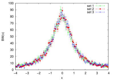
Figure 1: Simulated data from the Breit-Wigner distribution. They are separated into the three subsets denoted by the different point styles.

If, for each subset, we denote by $B_{i}$ and $\sigma_{B,i}$ the content and the statistical uncertainty of the $i^{th}$ histogram bin,

the bootstrapped data are given by Eq. (12), where the experimental values $E_{i}$ and $\sigma_{i}$ are replaced by $B_{i}$ and $\sigma_{B,i}$, i.e.

$$\mathcal{B}_{ij}=(1+\delta_{ij})\left[B_{i}+\gamma_{ij}\sigma_{B,i}\right].$$ (35)

We are able now to implement our new fit method and to check it in different conditions:

• 3 fit parameters ($I$, $\mu$ and $\Gamma$), labeled as Fit_3p;

• 2 fit parameters ($I$ and $\Gamma$), and one fixed parameter ($\mu=\mu_{0}$), labeled as Fit_2p+1f;

• 2 fit parameters ($I$ and $\Gamma$), and one sampled parameter ($\mu\in\mathcal{N}[\mu_{0},\sigma^{2}_{\mu_{0}}]$), labeled as Fit_2p+1s. The $\sigma_{\mu_{0}}$ term is chosen as $k/100$, where $k=3,20$ in order to investigate how the size of the uncertainties on $\bm{\psi}$ affects the fit results.

We also assume that each subset is affected by uniformly distributed systematic scale uncertainty with: $\Delta_{1}=0.04$, $\Delta_{2}=0.06$ and $\Delta_{3}=0.03$.

The number $N$ of bootstrap replicas to be generated is evaluated in the Fit_3p case, and without the inclusion of systematic uncertainties, with the goal to to obtain a relative precision $e_{r}\leq 5\%$ (in rms units) on the central values of all fit parameters. Under these conditions, as shown in FIG. 2, the $\mu$ parameter has, for a given $N$, the highest $e_{r}$ value and reaches the required precision at $N\simeq 10000$.

For each condition, the fit is then performed with 10000 bootstrap replicas both without and with the inclusion of the systematic uncertainties. In the first case we simply set $\delta_{ij}=0$ in Eq. (12) and Eq. (35), while in the second one we add the superscript ^′ to every fit condition.

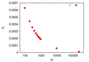
(a)

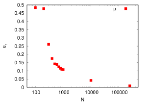
(b)

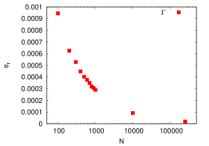
(c)

Figure 2: Relative error $e_{r}$ (in rms units) on the central values of the fit parameters $I$ (a), $\mu$ (b) and $\Gamma$ (c) as a function of the number of bootstrap cycles $N$.

III.2 Fit results

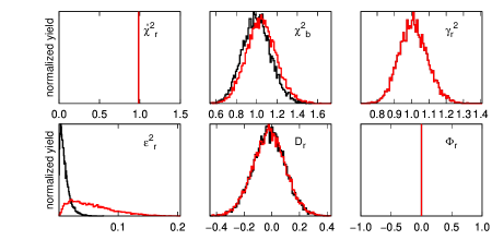
Figure 6: Decomposition of the $\hat{\chi}^{2}_{b,j}$ parameter in the Fit_3p configuration when systematic uncertainties are excluded (black curves) and included (red curves). Upper panel (from left to right): $\hat{\chi}^{2}_{r}$, $\chi_{b}^{2}$ and $\gamma^{2}_{r}$ components. Lower panel (from left to right): $\epsilon^{2}_{r}$, $D_{r}$ and $\Phi_{r}$ components. See text (and, in particular, Eq. (II.3), Tables 1 and 2) for the notation and the expected values of the different components. Black and red lines exactly overlap for the constant $\hat{\chi}^{2}_{r}$ and $\Phi_{r}$ components.

The final results of the fit performed under all the conditions described above are displayed in Table 1 and the obtained distributions of the fit parameters are shown in FIGs. 3 and 4. The expected values (labeled as $\mathbb{E}\left[\dots\right]$) and the distributions of the different components of ${\hat{\chi}^{2}_{b,j}}$ and ${\hat{\chi}^{2}_{th,j}}$ (see Eq. (II.3) for notation) are given in Table 2 and FIGs. 6 to 9, respectively. Finally, the CDFs of the expected goodness-of-fit distributions are displayed in FIGs. 10 and 11, respectively. In the following a detailed discussion of all these results is given.

DATA
Fitting conditions	$I$	$\mu$ $(10^{-3})$	$\Gamma$ ($10^{-1}$)	$\hat{\chi}^{2}_{r}$	$p$-value	Symbol
Fit3p	${247.0}^{+1.4}_{-1.5}$	${1.8}^{+7.1}_{-7.6}$	${9.8}\pm 0.1$	$0.98$	$45\%$	${\color[rgb]{0,0,0}\circ}$
Fit${}_{3p}^{\prime}$	${247.0}^{+4.0}_{-4.2}$	${1.8}^{+7.1}_{-7.7}$	${9.8}\pm 0.1$	$0.98$	$35\%$	${\color[rgb]{1,0,0}\circ}$
Fit2p+1f	${247.0}^{+1.4}_{-1.5}$	fixed	${9.8}\pm 0.1$	$0.98$	$43\%$
Fit${}_{2p+1f}^{\prime}$	${247.0}^{+4.0}_{-4.2}$	fixed	${9.8}\pm 0.1$	$0.98$	$34\%$
Fit2p+1s ($3\%$)	${247.0}^{+1.4}_{-1.5}$	sampled	${9.8}\pm 0.1$	$0.98$	$43\%$
Fit${}_{2p+1s}^{\prime}$ ($3\%$)	${247.0}^{+3.9}_{-4.3}$	sampled	$9.8\pm 0.1$	$0.98$	$34\%$
Fit2p+1s ($20\%$)	${243.0}^{+4.2}_{-5.0}$	sampled	${10.0}^{+0.2}_{-0.3}$	$1.05$	$25\%$
Fit${}_{2p+1s}^{\prime}$ ($20\%$)	${242.0}^{+5.9}_{-6.2}$	sampled	${10.0}^{+0.2}_{-0.3}$	$1.05$	$19\%$

Table 1: Results from the fit applied to the simulated data in the different conditions described in the text. Each $p$-value is calculated from the expected goodness-of-fit distribution, which is reconstructed in the framework of the bootstrap technique. The superscript ^′ denotes the inclusion of systematic uncertainities in the fit procedure and the different symbols refer to the point styles of FIGs. 3 and 4.

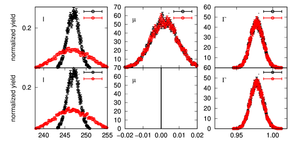
Figure 3: Probability distributions for the fit parameters of the simulated data for the Fit(’)_3p (upper panels) and Fit(’)_2p+1f (lower panels) configurations. From left to right: the scale factor $I$, the mean $\mu$ and the width $\Gamma$. The red (black) points indicate the inclusion (exclusion) of the systematic uncertainties in the fit procedure. In the Fit_2p+1f case, the mean value $\mu$ is not fitted but kept fixed to zero. See Table 1 for the meaning of the symbols.

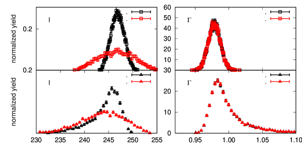
Figure 4: Probability distributions for the fit parameters of the simulated data for the Fit(’)_2p+1s($3\%$) (upper panels) and Fit(’)_2p+1s($20\%$) (lower panels) configurations. From left to right: the scale factor $I$ and the width $\Gamma$. The red (black) points indicate the inclusion (exclusion) of the systematic uncertainties in the fit procedure. The mean value $\mu$ is not shown here, being sampled from its known value $\mu_{0}$. See Table 1 for the meaning of the symbols.

III.2.1 Fit_3p

As a first consistency check, we compare the results obtained in this condition, shown in first line of Table 1, to the results from the standard fit procedure (see Eqs. (1) and (2)), which gives:

$$I=247.0\pm 1.5,\quad\mu=(1.7\pm 7.4)\cdot 10^{-3},\quad\Gamma=(9.8\pm 0.1)\cdot 10^{-1},\quad\hat{\chi}_{r}^{2}=0.98.$$ (36)

All these values are in very good agreement with the numerical results of Table 1. The only small difference is the asymmetry of the bootstrapped 1-$\sigma$ interval for $I$ and $\mu$. This feature is due to both the finite number of replicas (10000) and to the finite number of bins (100) of the histograms used for the evaluation of the CDF for the goodness-of-fit distribution.

Such a difference can be reduced by increasing the number of bootstrap cycles and of the classes used for the CDFs generation. As an example, when using 100000 replicas and 200-bin histograms, we obtain exactly the same confidence intervals as in the standard procedure.

This approximation can also be taken under control by examining the empirical probability distribution functions shown by the black open dots of FIG. 3 (upper panels). Using a standard best-fit procedure, we checked that they follow a Gaussian distribution, in agreement with statistical expectations (see, for instance, James (2006)). As an example, the probability distribution of the fit parameter $I$ obtained with 100000 bootstrap replicas is shown in the left plot of FIG. 5 and compared to the best-fit Gaussian distribution. Using the output fit parameters, we obtain exactly the same 1-$\sigma$ range given in Eq. (36).

The expected values and the distributions of the different components of ${\hat{\chi}^{2}_{b,j}}$ (see Eq. (20)), are given in the first line of Table 2 (upper part) and in the upper panel of FIG. 6 (black curves), respectively. The statistical fluctuations of ${\hat{\chi}^{2}_{b,j}}$ are almost entirely due to the $\gamma^{2}_{r}$ term, since the contributions given by $\epsilon_{r}^{2}$ and $D_{r}$ are quite small and the values of $\mathbb{E}\left[\epsilon_{r}^{2}\right]$ and $\mathbb{E}\left[D_{r}\right]$ are $O(10^{-2})$ and almost negligible.

In the ${\hat{\chi}^{2}_{th,j}}$ case (see Eq. (26) and FIG. 7), the term $\mathbb{E}\left[\hat{\chi}^{2}\right]$ is numerically very close to zero (see Table 2) and its distribution coincides with the reduced $\chi^{2}$-distribution, as expected from Eq. (II.3), due to the quite small and almost opposite values of $\mathbb{E}\left[\epsilon^{\prime}\right]$ and $\mathbb{E}\left[D^{\prime}_{r}\right]$. This result is shown by the black points in the left plot of FIG. 10.

All these properties fully confirm the considerations outlined in Section II.2 and Section II.3.

III.2.2 Fit${}_{3p}^{\prime}$

Due to the functional form of the BW distribution in Eq. (33), a common scale uncertainty only affects the uncertainty of $I$ and does not influence the estimate of the other parameters $\mu$ and $\Gamma$, as shown in the second line of Table 1 and in FIG. 3 (top panels).

We can compare these results to the ones obtained using the $\chi^{2}_{mod}$ function of Eq. (3), leaving the normalization factors for each subset as additional free parameters:

$$\chi^{2}_{mod}=\sum_{k}\left\{\left[\sum_{i\in\text{ set k}}\left(\frac{f_{k}E_{i}-T_{i}}{f_{k}\sigma_{i}}\right)^{2}\right]+\left(\frac{f_{k}-1}{\sigma^{\text{sys}}_{k}}\right)^{2}\right\},$$ (37)

where $\sigma^{\text{sys}}_{k}=\Delta_{k}/\sqrt{3},k=1,2,3$. In this case we obtain:

$$I=246.7\pm 3.5,\quad\mu=(1.7\pm 7.5)\cdot 10^{-3},\quad\Gamma=(9.8\pm 0.1)\cdot 10^{-1},\quad\hat{\chi}_{r}^{2}=0.99.$$ (38)

These results are very similar to the ones obtained under the Fit${}_{3p}^{\prime}$ configuration. The slightly smaller uncertainty on $I$ is mainly due to the fact that, as previously discussed, Eq. (37) should only be applied in the case of Gaussian systematic uncertainties.

This underestimation can be clearly seen if we closely examine the probability distribution for the fit parameter $I$, the only one that is significantly affected by the inclusion of the systematic uncertainties in the fit procedure. This study is also interesting since we cannot make any general assumption about its functional form and our method empirically provides its shape.

The obtained distribution with 100000 bootstrap cycles is shown in the central plot of FIG. 5, where we can clearly notice a significant deviation from the pure Gaussian shape obtained when systematic undertainties are neglected (left plot of of FIG. 5). The simple Gaussian best-fit (solid blue line) gives for $I$ the same confidence interval of Eq. (38), thus underestimating the true rms value. Such a discrepancy becomes more relevant as the value of $\Delta_{k}$ is artificially increased, as shown in right plot of FIG. 5. This behavior can be qualitatively explained by the fact that, given the sampling defined in Eq. (12), the distribution of the $I$ parameter results from the convolution of a uniform and a Gaussian function, with its shape depending on the $\Delta_{k}/\sigma_{i}$ ratio.

Within the frequentist framework, the correct solution can be found using the ML approach and by finding the parameter values that maximize:

$$\mathcal{L}_{unif}=\sum_{k}\left\{\prod_{i\in\text{ set k}}\left[\frac{1}{\sigma^{2}_{i}\sqrt{2\pi}}e^{-\frac{(f_{k}E_{i}-T_{i}(\bm{\theta}))^{2}}{2f_{k}\sigma^{2}_{i}}}\right]\cdot\mathcal{U}[-\Delta_{k},\Delta_{k}]\right\}.$$ (39)

As an alternative, the HBM model (see de Souza et al. (2019)) can also be used. In this framework, $\mathcal{L}_{unif}$ can be rewitten as:

$$\mathcal{L}_{unif}\equiv\mathcal{L}(E_{i}|\bm{\theta,f})\pi(\bm{f})\ ,$$ (40)

where $\mathcal{L}(E_{i}|\bm{\theta,f})$ is the probability to obtain the experimental data for a given set of model parameter values and $\pi(\bm{f})$ is the prior distribution for the parameters $\bm{f}$. When a uniform non-informative prior distribution is taken for the other fit parameters $\bm{\theta}$, we can write:

$$p(\bm{\theta,f}|E_{i})\propto\mathcal{L}_{unif}\ ,$$ (41)

where $p(\bm{\theta,f}|E_{i})$ is the posterior probability of a specific set of model parameter given the data.

Under these conditions, the 68% Bayesian credible intervals for the fit parameters obtained from HBM and using a Markov chain Monte Carlo procedure are:

$$I=246.6^{+4.0}_{-4.1},\quad\mu=(1.7^{+6.6}_{-7.0})\cdot 10^{-3},\quad\Gamma=(9.8\pm 0.1)\cdot 10^{-1}.$$ (42)

These values are in very good agreement with the ones given in Table 1 and also the distributions for all the fit parameters are the same as the ones shown in FIG. 3 and in the central plot of FIG. 5. All these conclusions give an important consistency check on the validity of our fit procedure.

Similarly to it, the HBM approach has also a very flexible implementation and can be used to easily model and reproduce a wide variety of uncertainty distribution. However, our method takes into account the effect of the systematic uncertainties without the need of additional fit parameters. This feature can give a sizable advantage in all those cases where a significanty large number of these parameters should be included in the fit procedure.

Finally, If we examine the ${\hat{\chi}^{2}_{b,j}}$ decomposition (red curves in the upper panel of FIG. 6) we note that there are additional statistical fluctuations due to the increased dispersion of the $\epsilon_{r}^{2}$ distribution (see also Table 2), even if $\mathbb{E}\left[\hat{\chi}^{\texttwosuperior}\right]$ has the same value as in the Fit_3p case. All this agrees to the results obtained with the $\chi^{2}_{mod}$ procedure.

Due to the correlations between the data caused by the systematic uncertainties, the expected goodness-of-fit distribution is now different from the reduced $\chi^{2}$-distribution. This feature can be clearly seen in a quantitative way in FIG. 7 (red curves), where both the ${\epsilon^{\prime}}^{2}_{r}$ and the $D^{\prime}_{r}$ term now give a significant contribution to ${\hat{\chi}^{2}_{th,j}}$, thus distorting the effect of the predominant $\gamma^{2}_{r}$ term. All these results are consistent with the considerations outlined in II.3 (see, in particular, Eq. (II.3)). The size of this distortion depends both on the magnitude of the systematic uncertainties and on the analytical structure of the model $T$.

The CDF for the goodness-of-fit distribution is shown by the red dots of FIG. 10 (left panel) and the resulting $p$-value (see Table 1) is significantly different from the Fit_3p case. All these considerations signal that this crucial fit parameter cannot be correctly evaluated within the $\chi^{2}_{mod}$ framework when the normalization uncertainties follow a distribution that differs substantially from the Gaussian one.

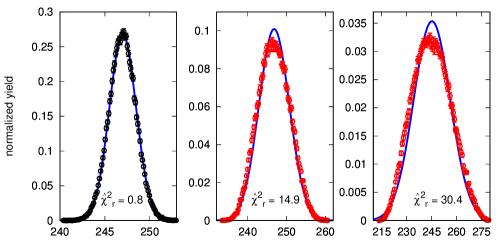
Figure 5: Probability distributions for the fit parameter $I$, obtained with 100000 bootstrap cycles and 100 histogram bins under the Fit_3p (left panel), Fit${}_{3p}^{\prime}$ (central panel) and Fit${}_{3p}^{\prime}$ with $3\cdot\Delta_{k}$ (right panel) configurations. These distributions are compared to the best-fit Gaussian curves (blue solid curves) and the corresponding $\hat{\chi}^{2}_{r}$ values are also given at the bottom of each plot.

III.2.3 Fit_2p+1f

As expected, all the results obtained in this case, both with and without the inclusion of the systematic uncertainties, are basically the same as in the Fit$(^{\prime})_{3p}$ conditions (see Table 1 and Table 2). They will be used as a benchmark to compare the results of the Fit$(^{\prime})_{2p+1s}$ conditions to quantitatively investigate the effects on the fit results given by the uncertainties related to additional model parameters.

III.2.4 Fit_2p+1s

The results obtained when $\sigma_{\mu_{0}}=3\%$ (fifth and sixth lines of Table 1 and Table 2, upper and lower parts of FIG. 8 and FIG. 11, left panel) are very similar to the ones obtained in the Fit$(^{\prime})_{2p+1f}$ conditions. The only relevant difference is the non-zero value of the $\mathbb{E}\left[\Phi\right]$ parameter. However, due to the small uncertainty assigned to the $\mu_{0}$ parameter, its effect is almost negligible. Also the probability distributions of the fit parameters $I$ and $\Gamma$ are still compatible with a Gaussian function.

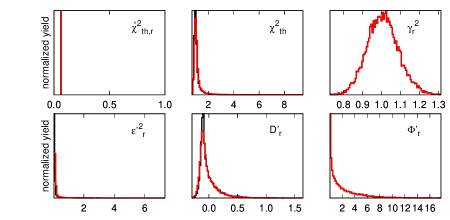
Figure 9: Decomposition of the $\hat{\chi}^{2}_{th,j}$ parameter for the Fit_2p+1s ($20\%$) configuration when systematic excluded (black curves) and included (red curves). Upper panel (from left to right): $\hat{\chi}^{2}_{th,r}$, $\chi^{2}_{th}$ and $\gamma^{2}_{r}$ components. Lower panel (from left to right): ${\epsilon^{\prime}}^{2}_{r}$, $D^{\prime}_{r}$ and $\Phi^{\prime}$ components. See text for the notation.

On the contrary, the fit results significantly change when $\sigma_{\mu_{0}}$ is large and equal to $20\%$, as shown in the seventh and eighth lines of Table 1 and Table 2, upper and lower parts, FIG. 9 and FIG. 11, right panel.

The probability distributions of the fit parameters $I$ and $\Gamma$ are strongly asymmetric and significantly different from all the previous cases. The $\Phi^{\prime}_{r}$ term gives a sizable contribution to ${\hat{\chi}^{2}_{th,j}}$ with a significant distortion of the goodness-of-fit distribution. Also the effect on the data systematic uncertainties is strongly reduced, as shown in FIG. 11, due to the effect of the relevant uncertainty on $\mu_{0}$. As previously mentioned (see Sec. II.3), in this case it would be more meaningful to add $\mu$ as an additional fit parameter.

DATA
Fitting conditions	$\mathbb{E}\left[\hat{\chi}^{2}_{r}\right]$	$\mathbb{E}\left[\gamma^{2}_{r}\right]$	$\mathbb{E}\left[\epsilon_{r}^{2}\right]$	$\mathbb{E}\left[D_{r}\right]$	$\mathbb{E}\left[\Phi_{r}\right]$
Fit3p	$0.98$	$1.01\pm 0.08$	$(9.92\pm 8.18)\cdot 10^{-3}$	$(-2.0\pm 11.6)\cdot 10^{-2}$	$0$
Fit${}_{3p}^{\prime}$	$0.98$	$1.01\pm 0.08$	$(5.55\pm 3.67)\cdot 10^{-2}$	$(-2.0\pm 11.9)\cdot 10^{-2}$	$0$
Fit2p+1f	$0.98$	$1.01\pm 0.08$	$(6.59\pm 6.65)\cdot 10^{-3}$	$(-1.3\pm 11.5)\cdot 10^{-2}$	$0$
Fit${}_{2p+1f}^{\prime}$	$0.98$	$1.01\pm 0.08$	$(5.20\pm 3.63)\cdot 10^{-2}$	$(-1.3\pm 11.8)\cdot 10^{-2}$	$0$
Fit2p+1s ($3\%$)	$0.98$	$1.01\pm 0.08$	$(6.76\pm 6.70)\cdot 10^{-3}$	$(-1.2\pm 11.5)\cdot 10^{-2}$	$(5.32\pm 7.99)\cdot 10^{-2}$
Fit${}_{2p+1s}^{\prime}$ ($3\%$)	$0.98$	$1.01\pm 0.08$	$(5.15\pm 3.58)\cdot 10^{-2}$	$(-1.2\pm 11.8)\cdot 10^{-2}$	$(5.32\pm 7.99)\cdot 10^{-2}$
Fit2p+1s ($20\%$)	$1.05$	$1.01\pm 0.08$	$(11.3\pm 32.4)\cdot 10^{-2}$	$(-1.5\pm 20.4)\cdot 10^{-2}$	$2.00\pm 2.47$
Fit${}_{2p+1s}^{\prime}$ ($20\%$)	$1.05$	$1.01\pm 0.08$	$(15.6\pm 32.2)\cdot 10^{-2}$	$(-1.8\pm 20.9)\cdot 10^{-2}$	$2.00\pm 2.47$
MODEL
Fitting conditions	$\mathbb{E}\left[\hat{\chi}_{th}^{2}\right]$	$\mathbb{E}\left[\gamma^{2}_{r}\right]$	$\mathbb{E}\left[{\epsilon^{\prime}}^{2}_{r}\right]$	$\mathbb{E}\left[D^{\prime}_{r}\right]$	$\mathbb{E}\left[\Phi_{r}^{\prime}\right]$
Fit3p	$\mathcal{O}(10^{-6})$	$1.01\pm 0.08$	$(9.96\pm 8.20)\cdot 10^{-3}$	$(-1.99\pm 1.64)\cdot 10^{-2}$	$0$
Fit${}_{3p}^{\prime}$	$\mathcal{O}(10^{-4})$	$1.01\pm 0.08$	$(5.66\pm 3.75)\cdot 10^{-2}$	$(-2.00\pm 3.02)\cdot 10^{-2}$	$0$
Fit2p+1f	$\mathcal{O}(10^{-7})$	$1.01\pm 0.08$	$(6.61\pm 6.67)\cdot 10^{-3}$	$(-1.32\pm 1.33)\cdot 10^{-2}$	$0$
Fit${}_{2p+1f}^{\prime}$	$\mathcal{O}(10^{-4})$	$1.01\pm 0.08$	$(5.32\pm 3.71)\cdot 10^{-2}$	$(-1.34\pm 2.86)\cdot 10^{-2}$	$0$
Fit2p+1s ($3\%$)	$\mathcal{O}(10^{-5})$	$1.01\pm 0.08$	$(6.78\pm 6.72)\cdot 10^{-3}$	$(-1.34\pm 1.33)\cdot 10^{-2}$	$(5.46\pm 8.16)\cdot 10^{-2}$
Fit${}_{2p+1s}^{\prime}$ ($3\%$)	$\mathcal{O}(10^{-4})$	$1.01\pm 0.08$	$(5.26\pm 3.67)\cdot 10^{-2}$	$(-1.39\pm 2.83)\cdot 10^{-2}$	$(5.46\pm 8.15)\cdot 10^{-2}$
Fit2p+1s ($20\%$)	$\mathcal{O}(10^{-1})$	$1.01\pm 0.08$	$(11.0\pm 31.6)\cdot 10^{-2}$	$(-1.6\pm 16.4)\cdot 10^{-2}$	$1.97\pm 2.43$
Fit${}_{2p+1s}^{\prime}$ ($20\%$)	$\mathcal{O}(10^{-1})$	$1.01\pm 0.08$	$(15.4\pm 31.4)\cdot 10^{-2}$	$(-1.9\pm 17.0)\cdot 10^{-2}$	$1.97\pm 2.43$

Table 2: The expected values, labeled as $\mathbb{E}\left[\dots\right]$ of the different components of ${\hat{\chi}^{2}_{b,j}}$ and ${\hat{\chi}^{2}_{th,j}}$ are given in the upper and lower panels, respectively. See Eq. (II.3) for notation. The different symbols refer to the point styles of FIGs. 10 and 11.

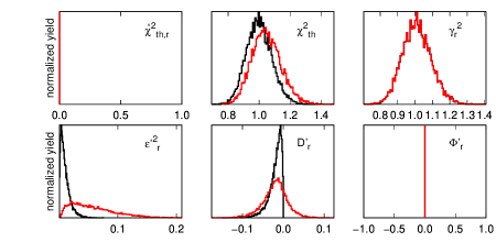
Figure 7: Decomposition of the $\hat{\chi}^{2}_{th,j}$ parameter in the Fit_3p configuration when systematic uncertainties are excluded (black curves) and included (red curves). Upper panel (from left to right): $\hat{\chi}^{2}_{th,r}$, $\chi^{2}_{th}$ and $\gamma^{2}_{r}$ components. Lower panel (from left to right): ${\epsilon^{\prime}}^{2}_{r}$, $D^{\prime}_{r}$ and $\Phi^{\prime}_{r}$ components. See text (and, in particular, Eq. (II.3), Tables 1 and 2) for the notation and the expected values of the different components. Black and red lines exactly overlap for the constant $\hat{\chi}^{2}_{th,r}$ and $\Phi^{\prime}_{r}$ components.

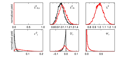
Figure 8: Decomposition of the $\hat{\chi}^{2}_{th,j}$ parameter in the Fit_2p+1s ($3\%$) configuration when systematic excluded (black curves) and included (red curves). Upper panel (from left to right): $\hat{\chi}^{2}_{th,r}$, $\chi^{2}_{th}$ and $\gamma^{2}_{r}$ components. Lower panel (from left to right): ${\epsilon^{\prime}}^{2}_{r}$, $D^{\prime}_{r}$ and $\Phi^{\prime}$ components. See text for the notation.

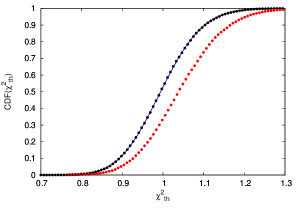
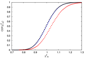
Figure 10: CDFs for the $\hat{\chi}^{2}_{r}$ parameter in the Fit_3p (left panel) and Fit_2p+1f configurations (right panel), when systematic uncertainties are included (red points) or discarded (black points). The solid blue line is the CDF of the reduced $\chi^{2}$-distribution.

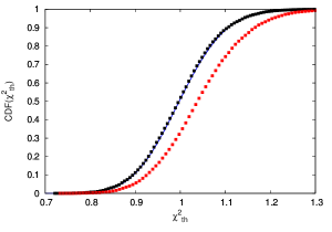
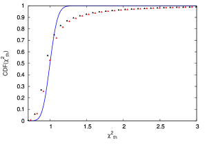
Figure 11: CDFs for the $\hat{\chi}^{2}_{r}$ parameter in the Fit_2p+1s ($3\%$) (left panel) and Fit_2p+1s ($20\%$) (right panel) configurations, when systematic uncertainties are included (red points) or discarded (black points). The solid blue line is a the CDF of a reduced $\chi^{2}$ distribution.

We finally notice that in the HBM framework there is no need to choose between this and Fit(’)_3p condition. Any prior knowledge of $\mu$, such as the one incorporated in Fit(’)_2p+1s, can be added to the Bayesian prior function $\pi$ defined in Eq. (41) and the final fit results will account for this additional information.

III.3 An additional complication: data with a systematic offset

We showed in the previous sections how to deal with the systematic uncertainties associated to the experimental data. However, we implicitly assumed that the data themselves are not affected by any intrinsic offset. We now make a step further and outline a strategy that allow us to deal with a priori unknown systematic offset of the data themselves.

Within our toy model, we assume that each data set has an unknown multiplicative offset $\delta_{k}^{*}$ lying inside the estimated uncertainty interval $[-\Delta_{k},\Delta_{k}]$. We then fix $\delta_{1}^{*}=3\%$, $\delta_{2}^{*}=4\%$ and $\delta_{3}^{*}=-2\%$ and artificially rescale all the points of the $k^{th}$ subset ($k=1,2,3)$ according to $E_{i}^{*}=(1+\delta^{*})E_{i}$ and $\sigma_{i}^{*}=(1+\delta^{*})\sigma_{i}$.

If now we apply the bootstrap method in the Fit_3p and Fit${}_{3p}^{\prime}$ conditions, we obtain, respectively:

$$\text{Fit${}_{3p}$: }I = 250.7^{+1.4}_{-1.5},\quad\mu=(1.9\pm 7.4)\cdot 10^{-3},\quad\Gamma=(9.8\pm 0.1)\cdot 10^{-1},\quad\hat{\chi}_{r}^{2}=1.07,\quad\text{$p$-value}=19\%,$$

$$\text{Fit${}_{3p}^{\prime}$: }I = 250.7\pm 4.0,\quad\mu=(1.9^{+7.2}_{-7.6})\cdot 10^{-3},\quad\Gamma=(9.8\pm 0.1)\cdot 10^{-1},\quad\hat{\chi}_{r}^{2}=1.07,\quad\text{$p$-value}=30\%.$$ (43)

Both the central values and the uncertainty intervals of the fit parameters are basically unchanged from the previous results given in Table 1, but the $\hat{\chi}_{r}^{2}$ value is now larger than before. Also the expected goodness-of-fit distribution, when systematic uncertainties are not taken into account, is different form the reduced $\chi^{2}$-distribution. This effect is already visible in FIG. 12 and, as expected, the discrepancy increases when $|\delta_{k}^{*}|$ increases.

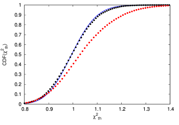
Figure 12: CDFs for the $\hat{\chi}^{2}_{r}$ parameter in the Fit${}_{3p}^{\prime}$ (red points) and Fit_3p (black points) configurations. The solid blue line is a the CDF of a reduced $\chi^{2}$ distribution.

If the model $T$ correctly reproduces the data, we can use the bootstrap framework also to estimate the unknown data offset with the following procedure:

1. apply the bootstrap fit in the Fit_3p condition and allow the parameter $\delta_{ij}$ to span a range wider than $[-\Delta_{k},\Delta_{k}]$ only for one chosen set and assuming that all other data sets do have any systematic offset. This choice is (at least partially) justified when several different and independent subsets have to be taken into account, since, in this case, the overall effect of the different biases should be small due to compensation effects.

2. the study of the behavior of the ${\hat{\chi}^{2}_{b,j}}$ parameter as a function of $\delta_{ij}$ allows one to find the value $\tilde{\delta}$ that gives the minimum value of $\mathbb{E}\left[\hat{\chi}^{2}_{b,j}(\delta_{ij})\right]$. Such a value can be taken as an estimate of the true, unknown data offset.

3. repeat the previous steps for each single subset to empirically evaluate all their different offsets.

The results of this strategy, where we choose to consider the offset only on set 1, are shown in FIG. 13(a) and Table 3, from which we can see that $\tilde{\delta}=-3.1\%\simeq-\delta_{1}^{*}$. By generating a sufficiently high number of points, the intrinsic error on $\tilde{\delta}$ can be made arbitrarily small (in our case it is of the order of $10^{-7}$).

This result means that if we want to force set 1 to be in good agreement with set 2 and set 3, we need to shift all its points back to their starting values, i.e. rescaling them by a factor $-\delta_{1}^{*}$.

This procedure is equivalent to use Eq. (37) and considering only the set 1 as affected by systematic uncertainties, i.e.

$$\chi^{2}_{mod,1}=\left[\sum_{\text{set 1}}\left(\frac{f_{1}E_{i}-T_{i}}{f_{1}\sigma_{i}}\right)^{2}\right]+\left[\sum_{\text{set 2,set 3}}\left(\frac{E_{i}-T_{i}}{\sigma_{i}}\right)^{2}\right]+\left(\frac{f_{1}-1}{\sigma^{\text{sys}}_{1}}\right)^{2},$$ (44)

thus obtaining $1-f_{1}=(2.60\pm 1.16)\%\simeq\delta_{1}^{*}$, as expected.

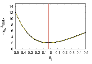
(a)

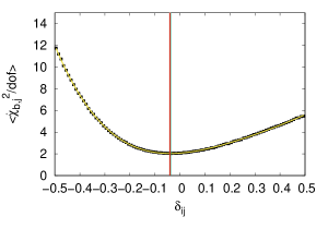
(b)

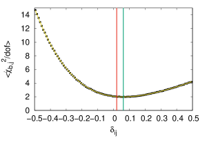
(c)

Figure 13: The $\mathbb{E}\left[{\hat{\chi}^{2}_{b,j}}\right]$ value as a function of $\delta_{ij}$. The black points are from the bootstrap technique, fitted with a fourth-order polynomial fit (yellow line). In each plot, the $\tilde{\delta}$ value is represented by the vertical green line, compared to the known $-\delta^{*}$ value (red line). The numerical results are given for subset 1 (a), 2 (b) and 3 (c).

Applying this strategy to subsets 2 and 3, we obtain the results shown in FIG. 13(b) and FIG. 13(c) and Table 3. They are compared to the results of the $\chi^{2}_{mod}$ approach both when the $f_{k}$ parameters are fitted one by one and when they are all fitted simultaneously (see Eq. (37)). Even if the $\tilde{\delta}_{k}$ parameters are not directly fitted in our procedure, their uncertainty intervals can be assigned using the so-called MINOS method (James (2006)), i.e. by finding the values of $\tilde{\delta}_{k}$ that cause $\mathbb{E}\left[{\hat{\chi}^{2}_{b,j}}\right]$ to vary by one unit. The numerical values of all these intervals are found to be coincident with the uncertainties resulting from the $\chi^{2}_{mod}$ approach.

From all these results, we can see that:

• the offsets of subsets 1 and 2 are well determined by this strategy, while there is a significant discrepancy between $\tilde{\delta}_{3}$ and $-\delta_{3}^{*}$. This disagreement is due to the fact that, as previously noted, when we estimate $\delta_{3}^{*}$, we are implicitly assuming that the other two subsets are not affected by any systematics, while they are both rescaled by the positive parameters $\delta_{1}^{*}$ and $\delta_{2}^{*}$ respectively. On the other hand, when we try to estimate $\delta_{1}^{*}$ or $\delta_{2}^{*}$, the other two subsets are rescaled according to systematics of different signs, thus introducing a compensation that allows us to (almost) correctly determine their value.

• the fit parameters obtained with the $\chi^{2}_{mod}$ procedure, i.e.

  $$I=247.7\pm 3.6,\quad\mu=(1.7\pm 7.5)\cdot 10^{-3},\quad\Gamma=0.98\pm 0.01,\quad\hat{\chi}_{mod,r}^{2}=1.01,$$ (45)

  are, within their estimated uncertainties, in agreement with the Fit${}_{3p}^{\prime}$ results shown in Table 1. However, we are not able to give a reliable $p$-value, since, as previously mentioned, the correlations among the data of each subset induced by the systematic uncertainties give a goodness-of-fit distribution different from the reduced $\chi^{2}$-function.

set number	known sys.	bootstrap	$\chi_{mod,r}^{2}$ (one-by-one)	$\chi_{mod,r}^{2}$ (simultaneous)
	$\delta_{k}^{*}$ ($\%$)	$-\tilde{\delta}_{k}$ ($\%$)	$1-f_{k}$ ($\%$)	$1-f_{k}$ ($\%$)
1	$3.0$	$3.1$	$2.2\pm 1.1$	$2.6\pm 1.5$
2	$4.0$	$3.8$	$3.2\pm 1.1$	$3.3\pm 1.6$
3	$-2.0$	$-6.2$	$-4.1\pm 1.0$	$-2.1\pm 1.4$

Table 3: Estimated offset values for each subset: results from the bootstrap (third column) and from the $\chi_{mod}^{2}$ method when the normalization factors $f_{k}$ are fitted one-by one (fourth column) or simultaneously (last column).

The bootstrap-based estimates of the real systematic offsets can be included into the fitting procedure in several ways. For instance, two alternative approaches are:

1. rescale all the data points and their statistical uncertainties by a factor $(1+\tilde{\delta}_{k})$ and perform a single minimization with the standard $\chi^{2}$ procedure. We then obtain:

   $$I=250.1\pm 1.5,\quad\mu=(1.4\pm 7.5)\cdot 10^{-3},\quad\Gamma=(9.8\pm 0.1)\cdot 10^{-1},\quad\hat{\chi}_{mod,r}^{2}=1.01,\quad\text{$p$-value }=46\%;$$ (46)

2. rescale the experimental data as described in the previous point and then apply the bootstrap fitting technique, setting $\delta_{ij}=0$ in Eq. (12). We now get:

   $$I=250.1\pm 1.5,\quad\mu=(1.6\pm 7.4)\cdot 10^{-3},\quad\Gamma=(9.8\pm 0.1)\cdot 10^{-1},\quad\hat{\chi}_{mod,r}^{2}=1.01,\quad\text{$p$-value }=45\%.$$ (47)

The results obtained in both the previous cases are very close, as expected, to the ones previously obtained in the Fit_3p condition.

IV A simplistic model with asymmetric statistical uncertainties

IV.1 Implementation

To provide an additional check of our new technique, we also apply our method to the case of asymmetric statistical uncertainties. This situation, that could be for instance due to a non-uniform background subtraction, is hardly treatable within the standard $\chi^{2}$ procedure.

To apply our method, we assume to have an experimental uncertainty distribution $f(x)$ described by the skew-Gaussian distribution (see, for instance, Azzalini (1985); Azzalini and Dalla Valle (1996)):

$$f(x)=\left({2}/{\omega}\right)g(z)G(\lambda z)\quad;\quad G(\lambda z)=\int_{-\infty}^{\lambda z}g(t)\,dt\ ,$$ (48)

where:

$$z=\frac{x-\xi}{\omega}\quad;\quad g(z)\sim\mathcal{N}[0,1]\ .$$ (49)

This function generalizes the usual Gaussian distribution to accomodate a certain amount of skewness. It is specified by 3 real-valued parameters: location($\xi$), scale ($\omega>0$) and shape ($\lambda$) with the usual Gaussian distribution corresponding to ($\lambda$=0). For each experimental point $E_{i}$, the $\lambda$, $\xi$ and $\omega$ parameters were choosen to be;

$$\lambda=-3\quad;\quad\xi=E_{i}-\omega\delta\sqrt{\frac{2}{\pi}}\quad,\quad\omega=\sigma_{i}\sqrt{1-\frac{2d}{\pi}}\ ,$$ (50)

where $d={\lambda}/{\sqrt{1+\lambda^{2}}}$. In this way we obtain:

$$\mathbb{E}\left[x\right]=E_{i}\quad;\quad\text{Var}\left[x\right]=\left(\sigma_{i}^{\text{stat}}\right)^{2}\ .$$ (51)

As an example, the skew-Gaussian distribution having zero mean, unit variance and $\lambda=-3$ is shown in FIG. 14 and compared to $\mathcal{N}[0,1]$.

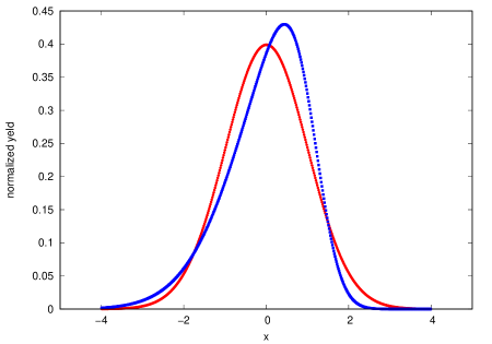
Figure 14: The probability density function of the skew-Gaussian distribution having zero mean, unit variance and $\lambda=-3$ (blue line) is compared to $\mathcal{N}[0,1]$ (red line).

This particular functional form was chosen since, even if it is asymmetric, we have:

$$\left(\frac{x-\xi}{\omega}\right)^{2}\sim\chi^{2}\ ,$$ (52)

independent of the value of $\lambda$. To a good approximation, the same relation also holds for $[({x-E_{i}})/{\sigma_{i}}]^{2}$ because, in our case $E_{i}\simeq\xi$ and $\sigma_{i}\simeq\omega$ (see Eq. (50)). This property then allows us to cross-check and validate the results we will obtain in this case with the ones found in the previous section.

IV.2 A generalised bootstrap formalism for $\hat{\chi}_{b,j}^{2}$

In the previous case, the bootstrap sampling can be written as (see Eqs. (12) and (13)):

$$\mathcal{B}_{ij}=(1+\delta_{ij})(E_{i}+s_{ij}),$$ (53)

where $s_{ij}$ is distributed according to a skew-Gaussian function having mean zero and variance $(\sigma^{exp}_{i})^{2}$. Using this notation, we can basically adopt almost the same decomposition shown in Sec. II.2. After introducing:

$$\rho_{ij}\equiv\frac{s_{ij}}{\sigma_{i}}\ ,$$ (54)

we only need to rewrite Eq. (II.2) as:

$$\tilde{D}_{ij} \equiv 2\left[\epsilon_{ij}\rho_{ij}+\frac{1}{\sigma_{i}}(\epsilon_{ij}+\rho_{ij})(E_{i}-T_{i}(\bm{\psi},\hat{\bm{\theta}}))\right],$$

$$\tilde{\Phi}_{ij} \equiv \eta_{ij}^{2}+2\eta_{ij}\left[(\epsilon_{ij}+\rho_{ij})+\frac{1}{\sigma_{i}}(E_{i}-T_{i}(\bm{\psi},\hat{\bm{\theta}}))\right],$$ (55)

where all the other parameters are defined as previously. After this small modification, the decomposition of $\hat{\chi}_{b,j}^{2}$ can be written in the same way as in Eq. (20), i.e.

$${\hat{\chi}^{2}_{b,j}}=\hat{\chi}^{2}+\sum_{i}\rho_{ij}^{2}+\sum_{i}\epsilon_{ij}^{2}+\sum_{i}\tilde{D}_{ij}+\sum_{i}\tilde{\Phi}_{ij}.$$ (56)

A very similar decomposition also holds for ${\hat{\chi}^{2}_{th,j}}$:

$${\hat{\chi}^{2}_{th,j}}=\hat{\chi}^{2}_{th}+\sum_{i}\rho_{ij}^{\prime 2}+\sum_{i}\epsilon_{ij}^{\prime 2}+\sum_{i}\tilde{D}^{\prime}_{ij}+\sum_{i}\tilde{\Phi}^{\prime}_{ij}.$$ (57)

thus allowing to rewrite all the components of Eq. (II.3) in the case of an asymmetric statistical error, with an obvious meaning for the $\tilde{\Phi}^{\prime}_{r}$, $\tilde{D}^{\prime}_{r}$ and $\rho_{r}^{\prime}$ parameters.

In this way, our bootstrap formalism can then be easily adapted to deal with any uncertainty distribution.

IV.3 Results

The results of the fit performed under the Fit(’) _3p condition are displayed in Table 4 and the correponding distributions for ${\hat{\chi}^{2}_{th,j}}$ and the the CDFs of the expected goodness-of-fit distributions are shown in FIGs. 15 and and 16, respectively. As expected, due to the symmetry properties of the skew-Gaussian function (see Eq. (52) and comments to it), all these results results are basically coincident with the ones shown in Table 1, FIGs. 7 and 10 (left plot).

DATA
Fitting conditions	$I$	$\mu$ $(10^{-3})$	$\Gamma$ ($10^{-1}$)	$\hat{\chi}^{2}_{r}$	$p$-value
Fit3p	${247.0}^{+1.4}_{-1.5}$	${1.8}^{+7.1}_{-7.6}$	${9.8}\pm 0.1$	$0.98$	$45\%$
Fit${}_{3p}^{\prime}$	${247.0}^{+4.0}_{-4.2}$	${1.8}^{+7.1}_{-7.7}$	${9.8}\pm 0.1$	$0.98$	$35\%$

Table 4: Results from the fit with skew-Gaussian statistical uncertainties in the Fit_3p and Fit${}_{3p}^{\prime}$ configurations.

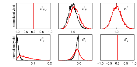
Figure 15: Decomposition of the $\hat{\chi}^{2}_{th,j}$ parameter with skew-Gaussian statistical uncertainties and in the Fit_3p configuration when systematic uncertainties are excluded (black curves) and included (red curves). Upper panel (from left to right): $\hat{\chi}^{2}_{th,r}$, $\chi^{2}_{th}$ and $\rho^{2}_{r}$ components. Lower panel (from left to right): ${\epsilon^{\prime}}^{2}_{r}$, $\tilde{D}^{\prime}_{r}$ and $\tilde{\Phi}^{\prime}_{r}$ components. See text for the notation. Black and red lines exactly overlap for the constant $\hat{\chi}^{2}_{th,r}$ and $\tilde{\Phi}^{\prime}_{r}$ components.

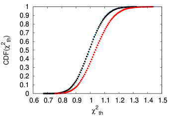
Figure 16: CDFs for the $\hat{\chi}^{2}_{r}$ parameter in the Fit${}_{3p}^{\prime}$ (red points) and Fit_3p (black points) configurations with skew-Gaussian statistical uncertainties. The solid blue line is a the CDF of a reduced $\chi^{2}$ distribution.

This very good agreement gives us confidence in the capability of our method to also correcty deal with asymmetric distributions.

V An application of the method: fit of real Compton scattering data

In this section we show an application of the bootstrap-based fitting method described in this work to an actual physics case: the extraction of the proton dipole scalar polarizabilities from the real Compton scattering (RCS) data, using fixed-$t$ subtracted dispersion relations Pasquini et al. (2018, 2019). In the RCS process, a real photon scatters off a proton, whose internal structure is probed when the photon energy is at least a few tens of MeV. The RCS differential cross section can be expressed, once the scattering angle and energy are fixed, in terms of 6 parameters, defined as the dipole scalar electric ($\alpha_{E1}$) and magnetic ($\beta_{M1}$) polarizabilities, and 4 vector spin-dependent polarizabilities ($\vec{\gamma}_{s}$). For a detailed description of RCS and the dispersion relation framework, the reader is addressed to Refs. Pasquini and Vanderhaeghen (2018); Drechsel et al. (1999); Pasquini et al. (2007); Drechsel et al. (2003) and references therein. For the purposes of this work, it is sufficient to recall that the RCS differential cross section $d\sigma/d\Omega$ can be written, once the photon scattering energy ($E_{\gamma}$) and angle ($\bm{\theta}_{\text{lab}}$) are fixed, as function of these 6 parameters, i.e. $d\sigma/d\Omega(\alpha_{E1},\beta_{M1},\vec{\gamma}_{s})$. The experimental set used for the fit is made of 150 data collected at $E_{\gamma}\leq 150$ MeV, and divided into 13 independent subsets as shown in Table 5.

set label	Ref.	first author	points number	$\bm{\theta}_{\text{lab}}$ (∘)	$E_{\gamma}$ (MeV)
1	Oxley (1958)	Oxley	4	$70-150$	$\simeq 60$
2	Hyman et al. (1959)	Hyman	12	$50,90$	$55-95$
3	Goldansky et al. (1960)	Goldansky	5	$75-150$	$55-80$
4	Bernardini et al. (1960)	Bernardini	2	$\simeq 135$	$\simeq 140$
5	Pugh et al. (1957)	Pugh	16	$50-135$	$40-120$
6	Baranov et al. (1974, 1975)	Baranov	3	$90,150$	$80-110$
7	Baranov et al. (1974, 1975)	Baranov	4	$90,150$	$80-110$
8	Federspiel et al. (1991)	Federspiel	16	$60,135$	$30-90$
9	Zieger et al. (1992)	Zieger	2	$180$	$100,130$
10	Hallin et al. (1993)	Hallin	13	$45-135$	$130-150$
11	MacGibbon et al. (1995)	MacGibbon	8	$90,135$	$95-145$
12	MacGibbon et al. (1995)	MacGibbon	10	$90,135$	$95-145$
13	Olmos de Leon et al. (2001)	Olmos de Leon	55	$60-155$	$60-150$

Table 5: Angular and energy coverage of the available experimental data on unpolarized cross section for proton RCS at $E_{\gamma}\leq 150$ MeV.

In Ref. Pasquini et al. (2019) the bootstrap-based technique outlined in this work has already been applied to extract $\alpha_{E1}$ and $\beta_{M1}$ from the fit of the RCS data listed above. In one of the cases analyzed in Ref. Pasquini et al. (2019), only the difference $(\alpha_{E1}-\beta_{M1})$ between the electric and magnetic polarizabilities was left as free parameter. The values of ($\alpha_{E1}+\beta_{M1}$) and of the remaining 4 spin-dependent polarizabilities $\vec{\gamma}_{s}$ were taken from the existing experimental estimates and the corresponding uncertainties were propagated into the fit procedure according to Eq. (15). This analysis gives as final result (see Pasquini et al. (2019)):

$$\alpha_{E1}=(12.03^{+0.48}_{-0.54})\times 10^{-4}\text{fm}^{3},\quad\beta_{M1}=(1.77^{+0.52}_{-0.54})\times 10^{-4}\text{fm}^{3},\quad\text{$p$-value}=12\%.$$ (58)

As an additional information about these fit outcomes, we show the estimate of the offset for each subset in the bootstrap framework (Sec. V.1) and the reconstructed goodness-of-fit distribution obtained in the fit conditions described above both with and without the inclusion of the systematic uncertainties (Sec. V.2).

V.1 Evaluation of the experimental bias

In this work, we adopt the same conditions as in Ref. Pasquini et al. (2019) and we apply the strategy discussed in Sec. III.3 to evaluate the offset values of the different subsets. The results of this analysis are shown in FIG. 17 and FIG. 18.

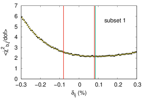
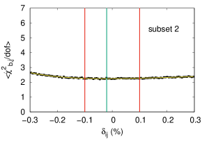
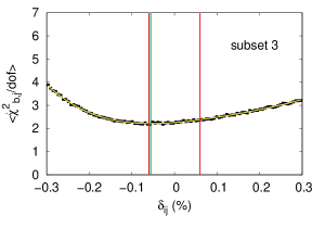
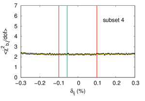
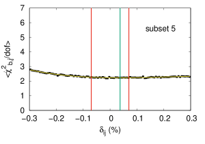
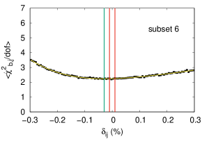
Figure 17: Estimate of $-{\delta}^{*}$ for data subsets from 1 to 6. In each plot, the black points are the results of the preliminary bootstrap cycle, the yellow curve gives the result of the quartic polynomial fit, the red curves are set at $\pm\Delta_{k}$ and the green line is set at $-{\delta}^{*}$.

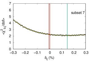
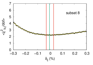
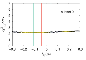
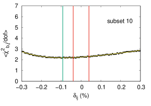
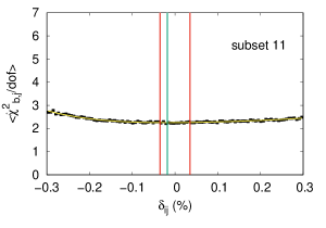
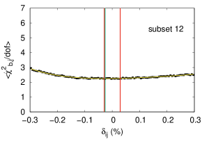
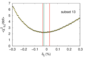
Figure 18: Estimate of $-{\delta}^{*}$ for data subsets from 7 to 13. In each plot, the black points are the results of the preliminary bootstrap cycle, the yellow curve gives the result of the quartic polynomial fit, the red curves are set at $\pm\Delta_{k}$ and the green line is set at $-{\delta}^{*}$.

Some comments are in order here:

• the subsets with very small number of points, or with points lying in kinematical regions not very sensitive to the fit parameter ($\alpha_{E1}$-$\beta_{M1}$), basically show a flat distribution. This means that the value of the systematic offset does not have a significant impact on the final fit results;

• for the majority of the subsets, the estimated systematic offset lies inside the published range, thus cross-checking the validity of the method;

• As mentioned before, this technique is model-dependent; for this reason, we do not recommend to use it to automatically discard data from the whole set. Even if the fit model $T$ is correct, when the evaluated offset value is outside the estimated systematic uncertainty interval, an ad hoc procedure is needed to correctly deal with each specific case.

In Table 6 the different values of the $\tilde{\delta}_{k}$ parameters determined for all the subsets are listed and compared to the $(f_{k}-1)$ parameters evaluated with the minimization of the modified $\chi^{2}$ function (see Eq. (3)). As done in Sec. III.3, the uncertainty intervals of the $\tilde{\delta}_{k}$ parameters can be estimated from the MINOS method. Also in this case we get very similar results as those obtained with the $\chi^{2}_{mod}$ approach.

The good agreement between these two sets of values gives a further indication of the correctness and validity of our new method. As noticed before, the offset estimate is now enough reliable due to the rather large number of data subsets.

Using the evaluated $\tilde{\delta_{k}}$ values, we can then rescale all the points of each subset by their estimated systematic offset and finally perform the bootstrap sampling taking only into account their statistical uncertainties, i.e.

$$\mathcal{S}_{ij}=(1+\tilde{\delta_{k}})(E_{i}+\gamma_{ij}\sigma_{i}),$$ (59)

where the only random numbers are the standard Gaussian variables $\gamma_{ij}$.

The results thus obtained for $\alpha_{E1}$ and $\beta_{M1}$ ( in the usual units of $10^{-4}\text{ fm}^{3}$, adopted from here on) are:

$$\alpha_{E1}=12.08\pm 0.24,\quad\beta_{M1}=1.69\pm 0.24,\quad\hat{\chi}_{r}^{2}=0.9,\quad\text{$p$-value }=20\%,$$ (60)

which are statistically consistent with the values that can be evaluated from a standard $\chi^{2}$ fit discarding all the systematic uncertainties, i.e.

$$\alpha_{E1}=11.99\pm 0.31,\quad\beta_{M1}=1.81\pm 0.31,\quad\hat{\chi}_{r}^{2}=1.25,\quad\text{$p$-value }=2\%.$$ (61)

If, on the other hand, we minimize the $\chi_{mod}^{2}$ function given in Eq. (3), we get:

$$\alpha_{E1}=11.94\pm 0.40,\quad\beta_{M1}=1.86\pm 0.40,\quad\hat{\chi}_{mod,r}^{2}=1.26,$$ (62)

which are, again, almost identical to the results obtained in the two previous cases.

k	$f_{k}-1$ $(\%)$	$\tilde{\delta}_{k}$ $(\%)$	k	$f_{k}-1$ $(\%)$	$\tilde{\delta}_{k}$ $(\%)$
1	$7.5\pm 2.3$	$8.6$	8	$0.0\pm 1.9$	$-0.4$
2	$-0.6\pm 4.8$	$-2.0$	9	$-4.7\pm 3.6$	$-11.6$
3	$-4.5\pm 2.1$	$-5.6$	10	$-5.7\pm 2.5$	$-9.2$
4	$-2.5\pm 6.5$	$-5.6$	11	$-0.4\pm 2.8$	$-1.7$
5	$3.0\pm 4.3$	$3.7$	12	$-0.7\pm 2.4$	$-2.6$
6	$-0.3\pm 0.9$	$-2.9$	13	$-0.1\pm 1.3$	$-2.1$
7	$7.5\pm 2.4$	$14.8$

Table 6: Estimate of the experimental offset for each data subset (labeled with $k$) used in the RCS analysis: results from the $\chi_{mod}^{2}$ method ($f_{k}-1$) are compared to the results of the bootstrap method ($\tilde{\delta}_{k}$).

It is noteworthy to observe that the statistical significance of the results substantially improves after the data rescaling (see Eqs. (60) and (61)). As already discussed in this work, the $p$-value can not be determined for the results given in Eq. (62), where the $\chi^{2}_{mod}$ procedure is used.

V.2 RCS: goodness-of-fit distribution

As mentioned before, in the RCS analysis of Ref. Pasquini et al. (2019) five parameters are sampled from their experimental estimates, while just one, i.e. the ($\alpha_{E1}-\beta_{M1}$) difference, is left as free parameter. This setting is quite similar to the previously described Fit_2p+1s case. Thus, after introducing the notations Fit_1p+5s (Fit${}_{1p+5s}^{\prime}$) for the exclusion (inclusion) of systematic uncertainties in the bootstrap sampling procedure, we can evaluate both the CDFs and the different components of ${\hat{\chi}^{2}_{th,j}}$ (see Eq. (II.3)).

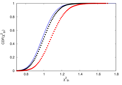
Figure 19: CDFs for the $\hat{\chi}^{2}_{th,j}$ parameter in the Fit_1p+5s (black points) and Fit${}_{1p+5s}^{\prime}$ (red points) conditions, compared to the CDF of the reduced $\chi^{2}$-distribution (solid blue curve). See Table 7 for the meaning of the symbols.

In the cumulative goodness-of-fit probability distribution shown in FIG. 19, the distortion caused by the inclusion of the systematic uncertainties is clearly visible. It is also interesting to note that, at odds with the results previously obtained with the toy model, the expected goodness-of-fit distribution is not the reduced $\chi^{2}$-function, even when the systematic uncertainties are excluded from the fit. As already noticed in Sec. III.3, this feature can be related to the non-negligible offsets present in the different data subsets. This effect can also be quantified with the $\mathbb{E}\left[{\epsilon^{\prime}}^{2}_{r}\right]$ and $\mathbb{E}\left[D^{\prime}_{r}\right]$ terms, which are not small enough to be ignored, even when only the statistical uncertainties are included in the analysis.

The expected values and the probability distributions of ${\hat{\chi}^{2}_{th,j}}$ are then given in Table 7 and FIG. 20 respectively, both switching on and off the systematic uncertainties.

MODEL
fitting conditions	$\mathbb{E}\left[\hat{\chi}^{2}_{r}\right]$	$\mathbb{E}\left[\gamma^{2}_{r}\right]$	$\mathbb{E}\left[{\epsilon^{\prime}}^{2}_{r}\right]$	$\mathbb{E}\left[D^{\prime}_{r}\right]$	$\mathbb{E}\left[\Phi\right]$	Symbol
Fit1p+5s	$10^{-6}$	$1.01\pm 0.11$	$(2.09\pm 2.97)\cdot 10^{-2}$	$(-1.30\pm 2.75)\cdot 10^{-2}$	$(3.62\pm 7.66)\cdot 10^{-2}$	${\color[rgb]{0,0,0}\bullet}$
Fit${}_{1p+5s}^{\prime}$	$10^{-6}$	$1.01\pm 0.11$	$(10.3\pm 4.8)\cdot 10^{-2}$	$(-1.35\pm 5.36)\cdot 10^{-2}$	$(3.62\pm 7.86)\cdot 10^{-2}$	${\color[rgb]{1,0,0}\bullet}$

Table 7: Decomposition of the $\hat{\chi}^{2}_{th,j}$ parameter, with the notation of Eq. (II.3), referred to the analysis of RCS proton data  Pasquini et al. (2019). The different symbols refer to the point styles of FIG. 19.

From the numerical values of Table 7, we can conclude that:

• the uncertainties on the fit parameter cannot be small, due to the relatively large values of the $\mathbb{E}\left[{\epsilon^{\prime}}^{2}_{r}\right]$ and $\mathbb{E}\left[D^{\prime}_{r}\right]$ ;

• the sampling of the additional nuisance parameters is under control, being the $\mathbb{E}\left[\Phi_{r}\right]$ small;

• the systematic uncertainties have a sizable effect on the fit uncertainties, being the $\mathbb{E}\left[{\epsilon^{\prime}}^{2}_{r}\right]$ term increased by a factor 5 as soon as they are included in the procedure.
  

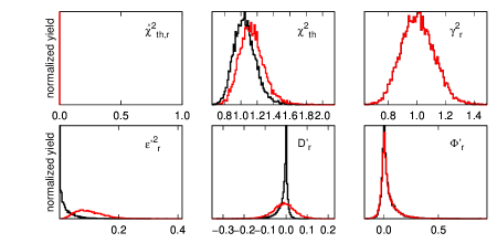
Figure 20: Decomposition of the $\hat{\chi}^{2}_{th,j}$ parameter for the Fit_1p+5s (black curves) and Fit${}_{1p+5s}^{\prime}$ (red curves) configurations. Upper panel (from left to right): $\hat{\chi}^{2}_{r}$, $\chi_{b}^{2}$ and $\gamma^{2}_{r}$ components. Lower panel (from left to right): $\epsilon_{r}^{2}$, the $D_{r}$ and $\Phi_{r}$ components. See text for the notation.

VI Conclusions

We presented a new fitting technique based on the parametric bootstrap method and we developed two different toy models to completely analyze and cross-check its main features using the results obtained both with the standard $\chi^{2}$ procedures and a Hierarchical Bayesian model. Furthermore, we applied the fitting technique to an actual physics process, i.e. the real Compton scattering off the proton Pasquini et al. (2019), thus confirming the portability of the technique itself.
We showed that this new technique offers several advantages when compared to the other procedures. The systematic uncertainties can be taken into account in a straightforward way without the need of additional fit parameters and with a very flexible implementation of any probability distribution. Furthermore, the probability distributions of the fit parameters are not assumed to be a priori Gaussian, but are empirically obtained by the procedure itself. Another advantage with respect to the standard best-fit methods is that the uncertainties on additional nuisance parameters can be easily taken into account, without resorting to the approximated, and often complicated to be implemented, error-propagation formula.
The bootstrap framework provides also an estimate of the overall offset of a given data set, giving results that are in very good agreement with the ones obtained from the standard $\chi_{mod}^{2}$ method. This feature can be used as an indication about the quality of the data points, but it should not be used as a fitting strategy by itself.
Furthermore, our fitting technique provides the correct $p$-value when systematic uncertainties are present and in all other cases when the goodness-of-fit distribution is not the reduced $\chi^{2}$-distribution.
All these benefits comw with one drawback: a relevant number of artificial bootstrap “measurements” has to be generated in order to well approximate both the (unknown) true probability distributions of the fit parameters and the fit $p$-value. Apart from this computational limitation, common to all the Monte Carlo-based methods, the previous considerations lead us to encourage the use of this technique.

VII Acknowledgments

We are very grateful to Barbara Pasquini, that provided all the theoretical framework for the analysis of the RCS data. We want to thank also Andrea Fontana, Alberto Rotondi, for stimulating discussions and Simone Rodini, for some useful suggestions. We also want to thank Lissa De Souza Campos for a careful reading of the manuscript.

References

- D’Agostini (1994) G. D’Agostini, Nucl. Instrum. Meth. A 346, 306 (1994).
- Gallego et al. (2013) G. Gallego, C. Cuevas, R. Mohedano, and N. Garcia, IEEE Trans. Signal Process. 61, 4387 (2013).
- de Souza et al. (2019) R. S. de Souza, S. R. Boston, A. Coc, and C. Iliadis, Phys. Rev. C99, 014619 (2019), arXiv:1901.04857 [nucl-th] .
- Pasquini et al. (2019) B. Pasquini, P. Pedroni, and S. Sconfietti, Journal of Physics G: Nuclear and Particle Physics (2019), 10.1088/1361-6471/ab323a.
- Davidson and Hinkley (1997) A. C. Davidson and D. V. Hinkley, Bootstrap Methods and their Application (Cambridge University Press, 1997).
- James (2006) F. James, Statistical methods in experimental physics (Hackensack, USA: World Scientific, 2006).
- Azzalini (1985) A. Azzalini, Scand. Jour. Stat. 12 (1985).
- Azzalini and Dalla Valle (1996) A. Azzalini and A. Dalla Valle, Biometrika 83, 715 (1996).
- D’Agostini (2003) G. D’Agostini, Bayesian reasoning in data analysis: A critical introduction (2003).
- D’Agostini (2004) G. D’Agostini, (2004), arXiv:physics/0403086 [physics] .
- Pasquini et al. (2018) B. Pasquini, P. Pedroni, and S. Sconfietti, Phys. Rev. C98, 015204 (2018), arXiv:1711.07401 [hep-ph] .
- Pasquini and Vanderhaeghen (2018) B. Pasquini and M. Vanderhaeghen, Ann. Rev. Nucl. Part. Sci. 68, 75 (2018), arXiv:1805.10482 [hep-ph] .
- Drechsel et al. (1999) D. Drechsel, M. Gorchtein, B. Pasquini, and M. Vanderhaeghen, Phys. Rev. C 61, 015204 (1999), arXiv:hep-ph/9904290 [hep-ph] .
- Pasquini et al. (2007) B. Pasquini, D. Drechsel, and M. Vanderhaeghen, Phys. Rev. C 76, 015203 (2007), arXiv:0705.0282 [hep-ph] .
- Drechsel et al. (2003) D. Drechsel, B. Pasquini, and M. Vanderhaeghen, Phys. Rept. 378, 99 (2003), arXiv:hep-ph/0212124 [hep-ph] .
- Oxley (1958) C. L. Oxley, Phys. Rev. 110, 733 (1958).
- Hyman et al. (1959) L. G. Hyman, R. Ely, D. H. Frisch, and M. A. Wahlig, Phys. Rev. Lett. 3, 93 (1959).
- Goldansky et al. (1960) V. Goldansky, O. Karpukhin, A. Kutsenko, and V. Pavlovskaya, Nuclear Physics 18, 473 (1960).
- Bernardini et al. (1960) G. Bernardini, A. O. Hanson, A. C. Odian, T. Yamagata, L. B. Auerbach, and I. Filosofo, Nuovo cim. 18, 1203 (1960).
- Pugh et al. (1957) G. E. Pugh, R. Gomez, D. H. Frisch, and G. S. Janes, Phys. Rev. 105, 982 (1957).
- Baranov et al. (1974) P. Baranov, G. Buinov, V. Godin, V. Kuznetzova, V. Petrunkin, Tatarinskaya, V. Shirthenko, L. Shtarkov, V. Yurtchenko, and Yu. Yanulis, Phys. Lett. 52B, 122 (1974).
- Baranov et al. (1975) P. S. Baranov, G. M. Buinov, V. G. Godin, V. A. Kuznetsova, V. A. Petrunkin, L. S. Tatarinskaya, V. S. Shirchenko, L. N. Shtarkov, V. V. Yurchenko, and Yu. P. Yanulis, Yad. Fiz. 21, 689 (1975).
- Federspiel et al. (1991) F. J. Federspiel, R. A. Eisenstein, M. A. Lucas, B. E. MacGibbon, K. Mellendorf, A. M. Nathan, A. O’Neill, and D. P. Wells, Phys. Rev. Lett. 67, 1511 (1991).
- Zieger et al. (1992) A. Zieger, R. Van de Vyver, D. Christmann, A. De Graeve, C. Van den Abeele, and B. Ziegler, Phys. Lett. B 278, 34 (1992).
- Hallin et al. (1993) E. L. Hallin et al., Phys. Rev. C 48, 1497 (1993).
- MacGibbon et al. (1995) B. E. MacGibbon, G. Garino, M. A. Lucas, A. M. Nathan, G. Feldman, and B. Dolbilkin, Phys. Rev. C 52, 2097 (1995), arXiv:nucl-ex/9507001 [nucl-ex] .
- Olmos de Leon et al. (2001) V. Olmos de Leon et al., Eur. Phys. J. A 10, 207 (2001).