Initial conditions for electron and photon structure and fragmentation functions

Abstract

In the computation of short-distance cross sections initiated by electrons and photons one can adopt the so-called structure-function approach, in which these particles play formally the same roles as hadrons do in QCD factorisation theorems, and must thus be associated with PDFs (equivalently known as structure functions in this context). At variance with their QCD counterparts, such PDFs are entirely calculable in QED. In this paper we present the results, at the next-to-leading order in the QED coupling constant $\alpha$, for the initial conditions of the unpolarised electron and photon PDFs, which are a necessary ingredient for their eventual collinear evolution at the next-to-leading logarithmic accuracy. We also compute the analogous final-state quantities, namely the initial conditions for fragmentation functions into electrons and photons.

1 Introduction

It is not unreasonable to assume that the medium- to long-term future of high-energy physics will involve an $e^{+}e^{-}$ collider. From the theoretical point of view, whether such a collider will be a linear or a circular one is relatively unimportant, since the primary goal will be that of computing production short-distance cross sections, which are independent of the collider type. What matters is that these cross sections are initiated by electrons and positrons (and, if beam dynamics play a significant role, by photons as well). We hasten to stress that although electrons/positrons and photons might feature in the initial states of hard reactions occurring at hadron colliders, the corresponding cross sections are fundamentally different with respect to their $e^{+}e^{-}$-collider counterparts. This is because in hadronic collisions leptons and photons emerge from the low-scale collinear and soft dynamics of the incoming hadrons; their momenta are not fixed, but distributed according to their respective Parton Distribution Functions (PDFs henceforth). Conversely, at an $e^{+}e^{-}$ collider, the incoming $e^{+}$, $e^{-}$, and $\gamma$ must be regarded as having definite and known momenta. Therefore, and at least when working in QED, physical distributions at $e^{+}e^{-}$ colliders can be obtained by using solely ingredients that can be computed from first principles, i.e. matrix elements and phase spaces.

The previous statement, if true, is however mostly academic when the computations are performed strictly in a perturbative series truncated at any given order in the QED coupling constant $\alpha$, because of the presence in the matrix elements of terms such as $\log^{k}E/m$, with $m$ the electron mass and $E$ a scale of the order of the hardness of the collision (e.g. the collider c.m. energy). These terms are numerically large and compensate the suppression due to the coupling constant, thus preventing the perturbative series from being well behaved. Fortunately, a large class of them is also process-independent, and can therefore be accounted for in a universal manner, thanks to the fact that their physical origin is well understood, and stem from collinear emissions off an electron/positron line: the finite electron mass screens potential collinear divergences, but leaves logarithmic leftovers. This is reminiscent of the situation in QCD, and one way to address the problem is indeed QCD-inspired: the structure-function approach Kuraev:1985hb ; Ellis:1986jba , whereby one collects all of the logarithmic terms in some universal factors (the PDFs, a.k.a. structure functions. Here, for brevity we shall mainly refer to them by the former name), which are then resummed by means of the DGLAP evolution equations Gribov:1972ri ; Lipatov:1974qm ; Altarelli:1977zs ; Dokshitzer:1977sg . The key difference w.r.t. QCD is that in QED one can calculate perturbatively not only the evolution kernels, which are the standard Altarelli-Parisi ones Altarelli:1977zs , but also the initial conditions for such an evolution.

The electron structure functions that are used nowadays result from the solution of the evolution equations where both the kernels and the initial conditions are leading-order (LO) accurate Skrzypek:1990qs ; Skrzypek:1992vk ; Cacciari:1992pz – at this order, the latter are in fact trivial, and equal to a Dirac delta. However, the accuracy targets of any future $e^{+}e^{-}$ collider must be matched by equally accurate theoretical computations, which thus demand to increase the precision of both the matrix element and the structure function predictions. The aim of this paper is to address the latter aspect, with the goal of calculating the initial conditions at the next-to-leading order (NLO) in QED; these are a prerequisite for an evolution accurate at the next-to-leading logarithmic (NLL) level BCCFS . When working at the NLO, the electron-photon mixing cannot formally be neglected any longer as is done at the LO; this applies to photon-initiated processes as well. Therefore, results will be presented for the initial conditions of all of the four possible combinations of electron and photons emerging from the collinear dynamics of either electron or photon evolution.

From the technical point of view, electron and photon structure functions are quite analogous to their final-state counterparts, namely to the fragmentation functions of either an electron or a photon emerging from the multiple collinear branchings of either an electron or a photon, which in turn are (some of) the outgoing particles of a hard scattering. Thus, we shall apply the methods employed in the case of the structure functions to compute the initial conditions for these fragmentation functions as well. Needless to say, owing to their being associated with final-state properties, these results will be equally relevant to lepton as to hadron colliders.

This paper is organised as follows: in sect. 2 we introduce the factorisation formulae which constitute the core of the structure function method. We shall employ two different procedures to compute the structure-function initial conditions, which we sketch in sect. 3; the corresponding calculations are reported in sects. 4 and 5, respectively. Initial conditions for fragmentation functions are presented in sect. 6. We summarise our results and draw our conclusions in sect. 7. Some technical material is collected in the appendices.

2 Cross sections and notation

At an $e^{+}e^{-}$ collider a generic differential cross section $d\Sigma_{e^{+}e^{-}}$ relevant to the process

$$e^{+}(P_{e^{+}})\,+e^{-}(P_{e^{-}})\;\longrightarrow\;X$$ (1)

is written as follows (throughout this paper, we sum over all polarisation states):

$$d\Sigma_{e^{+}e^{-}}(P_{e^{+}},P_{e^{-}})=\sum_{kl}\int dy_{+}dy_{-}\,{\cal B}_{kl}(y_{+},y_{-})\,d\sigma_{kl}(y_{+}P_{e^{+}},y_{-}P_{e^{-}})\,,$$ (2)

with

$$k\;\in\;\{e^{+},\gamma\}\,,\;\;\;\;\;\;\;\;l\;\in\;\{e^{-},\gamma\}\,.$$ (3)

In eq. (1) $X$ denotes a set of final-state particles, which does not play any role in what follows, and it is thus ignored notation-wise. The functions ${\cal B}_{kl}$ parametrise the beam dynamics, in particular beamstrahlung effects. Their forms are typically extracted from fits to Monte Carlo simulations, and are strictly dependent on the collider one considers; they also will play no role in this paper. Thus, eq. (2) is relevant here only insofar that it shows how the measured cross section is the incoherent sum of four terms, associated with short-distance cross sections $d\sigma_{kl}$ whose initial states are $e^{+}e^{-}$, $e^{+}\gamma$, $\gamma e^{-}$, and $\gamma\gamma$ pairs. As far as the latter cross sections are concerned, in the so-called structure-function approach one writes them in a way analogous to that of factorisation theorems in QCD, namely (see e.g. appendix A.1 of ref. Beenakker:1996kt ):

$$d\sigma_{kl}(\bar{p}_{k},\bar{p}_{l}) = \sum_{ij}\int dz_{+}dz_{-}\,\Gamma_{\!i/k}(z_{+},\mu^{2},m^{2})\,\Gamma_{\!j/l}(z_{-},\mu^{2},m^{2})$$ (4)

$$\phantom{\sum_{ij}\int}\times d\hat{\sigma}_{ij}(z_{+}\bar{p}_{k},z_{-}\bar{p}_{l},\mu^{2},m^{2})\,,$$

with $d\hat{\sigma}_{ij}$ a suitably defined quantity, which we shall specify later. By $m$ we have denoted the electron mass, $\mu$ is an arbitrary mass scale $\mu\gg m$, the indices $i$ and $j$ are such that

$$i\,,j\;\in\;\{e^{+},e^{-},\gamma\}\,,$$ (5)

and

$$\bar{p}_{q}=m_{q}^{2}\,,\;\;\;\;\;\;s=(\bar{p}_{k}+\bar{p}_{l})^{2}\,,$$ (6)

with either $m_{q}=m$ (when $q=e^{\pm}$) or $m_{q}=0$ (when $q=\gamma$). Two observations are in order. Firstly, the specific values assumed by the indices $i$ and $j$ are possibly subsets of those in eq. (5), that depend on both the incoming particles $k$ and $l$, and the perturbative order one is working at. Regardless of this, and consistently with what has been done for beamstrahlung effects, $\mu$ and $\tau$ contributions are ignored (lifting this limitation is straightforward, but it complicates the notation unnecessarily). Secondly, strictly speaking there is a kinematical inconsistency when eq. (4) is used in eq. (2), owing to eq. (6) and $P_{e^{\pm}}^{2}=m^{2}$. This is however irrelevant, since we shall show that factorisation formulae such as eq. (4) are best employed with massless incoming momenta (as is done in QCD). We shall often adopt a shorthand notation for eq. (4), which we write as follows:

$$d\sigma_{kl}=\sum_{ij}\Gamma_{\!i/k}\star\Gamma_{\!j/l}\star d\hat{\sigma}_{ij}\,.$$ (7)

The idea behind eq. (4) is that the cross section for the process of eq. (1) will depend on ratios such as:

$$\frac{m^{2}}{Q^{2}}\,,\;\;\;\;\;\;\;\;Q^{2}\sim s\,,$$ (8)

which might spoil the perturbative “convergence” since $m^{2}\ll s$. One then collects the universal dependence on the ratio (8) in the Initial-State Radiation (ISR) structure functions $\Gamma_{\!i/k}$ (which, owing to the strict analogy of eq. (4) with the QCD case, we shall call PDFs henceforth), and resums large logarithmic terms (at least, those of collinear origin) by means of the DGLAP evolution equations:

$$\frac{\partial\Gamma_{\!i/k}}{\partial\log\mu^{2}}=\frac{\alpha}{2\pi}P_{ij}\otimes\Gamma_{\!j/k}\,.$$ (9)

At any given perturbative order $\alpha^{u}$, the universal dependence of the cross section on $m^{2}/Q^{2}$ can be identified with logarithms of this ratio, times the cross section of order $\alpha^{u-1}$ with all such logarithms already removed. This definition is always arbitrary to a certain extent, which is why one introduces the scale $\mu$; note, however, that $\mu^{2}\sim s$. Furthermore, from now onwards we shall understand the rightmost relationship in eq. (8), and simply write $m^{2}/s$ to denote a generic “small” ratio.

While this is all fully analogous to its QCD counterpart, the key difference is that the PDFs $\Gamma_{\!i/k}$ are perturbatively calculable in QED. Indeed, they are available in a closed form to leading logarithmic (LL) accuracy, which account also for soft-photon effects Skrzypek:1990qs ; Skrzypek:1992vk ; Cacciari:1992pz . By expanding such a closed form in a series of $\alpha$, and by replacing the result thus obtained in eq. (4), one can solve for the subtracted cross sections $d\hat{\sigma}_{ij}$. This subtraction is mandatory, lest one double-count the universal terms already included in the PDFs. When working at the NLO, one uses the following expansions:

$$\Gamma_{\!i/k} = \Gamma_{\!i/k}^{[0]}+\frac{\alpha}{2\pi}\,\Gamma_{\!i/k}^{[1]}+{\cal O}(\alpha^{2})\,,$$ (10)

$$d\sigma_{kl} = d\sigma_{kl}^{[0]}+\frac{\alpha}{2\pi}\,d\sigma_{kl}^{[1]}+{\cal O}(\alpha^{2})\,,$$ (11)

$$d\hat{\sigma}_{ij} = d\hat{\sigma}_{ij}^{[0]}+\frac{\alpha}{2\pi}\,d\hat{\sigma}_{ij}^{[1]}+{\cal O}(\alpha^{2})\,.$$ (12)

By replacing these expressions into eq. (7) and by solving order by order in $\alpha$, one obtains:

$$d\sigma_{kl}^{[0]}=\sum_{ij}\Gamma_{\!i/k}^{[0]}\star\Gamma_{\!j/l}^{[0]}\star d\hat{\sigma}_{ij}^{[0]}$$ (13)

at ${\cal O}(\alpha^{0})$ (relative to the power of $\alpha$ implicit in the Born contribution), and:

$$d\sigma_{kl}^{[1]}=\sum_{ij}\left(\Gamma_{\!i/k}^{[1]}\star\Gamma_{\!j/l}^{[0]}\star d\hat{\sigma}_{ij}^{[0]}+\Gamma_{\!i/k}^{[0]}\star\Gamma_{\!j/l}^{[1]}\star d\hat{\sigma}_{ij}^{[0]}+\Gamma_{\!i/k}^{[0]}\star\Gamma_{\!j/l}^{[0]}\star d\hat{\sigma}_{ij}^{[1]}\right)$$ (14)

at ${\cal O}(\alpha)$. Whatever the form of $\Gamma_{\!i/k}$, it must be such that the physically-obvious zeroth-order condition

$$\Gamma_{\!i/k}^{[0]}(z,\mu^{2},m^{2})=\delta_{ik}\,\delta(1-z)$$ (15)

is fulfilled. Therefore, from eq. (13):

$$d\hat{\sigma}_{kl}^{[0]}=d\sigma_{kl}^{[0]}\,.$$ (16)

In fact, one can arrive at eq. (16) without employing eq. (15), by means of physical considerations: at the leading order, there are no logarithmic terms, and any mass dependence (bar for that in the flux, upon which we shall comment later) is specific to the process considered, and thus non-universal. Therefore, the subtracted cross section must be identical to the cross section that emerges directly from matrix element and phase space computations. As far as the ${\cal O}(\alpha)$ term is concerned, from eqs. (14) and (15) we obtain:

$$d\hat{\sigma}_{kl}^{[1]}=d\sigma_{kl}^{[1]}-\sum_{i}\left(\Gamma_{\!i/k}^{[1]}\star d\hat{\sigma}_{il}^{[0]}+\Gamma_{\!i/l}^{[1]}\star d\hat{\sigma}_{ki}^{[0]}\right)\,.$$ (17)

In order to clarify a physics argument that stems from eqs. (16) and (17), let us introduce the following naming conventions:

• $d\Sigma_{e^{+}e^{-}}$: collider-level cross section.

• $d\sigma_{kl}$: particle-level cross section.

• $d\hat{\sigma}_{ij}$: (subtracted) parton-level cross section.

Thus, in eqs. (2) and (4), $k$ and $l$ are particle indices, while $i$ and $j$ are parton indices. This might be confusing, since all of these indices assume the same values (see eqs. (3) and (5)). The possible confusion ultimately originates from the fact that an $e^{\pm}$ or $\gamma$ plays a double role in the context of the structure-function approach. Namely, it can be one of the objects that emerge from the beamstrahlung process, and is thus one of the incoming particles in the cross section on the r.h.s. of eq. (2) or the l.h.s. of eq. (4). But it can also be an object that emerges from the PDF evolution (i.e. from ISR), and is thus one of the incoming partons in the cross section on the r.h.s. of eq. (4).

This duality is not without practical consequences. In particular, eq. (16) and (17) must be interpreted as definitions of the subtracted partonic cross sections only when the parton indices coincide with the particle indices. While this is a trivial statement as far as eq. (16) is concerned (since there is actually no subtraction in that equation), it is not for eq. (17). Indeed, strictly speaking eq. (17) should be supplemented by:

$$d\hat{\sigma}_{ij}^{[1]}=d\sigma_{ij}^{[1]}\,,\;\;\;\;\;\;i\neq k~{}~{}{\rm or/and}~{}~{}j\neq l\,,$$ (18)

for any given particle indices $k$ and $l$. Thus, a partonic cross section will have, or will not have, to be subtracted depending on the particle cross section it contributes to. For examples, $d\hat{\sigma}_{\gamma e^{-}}^{[1]}$ will be derived from $d\sigma_{\gamma e^{-}}^{[1]}$ according to eq. (17) if contributing to the particle cross section initiated by a $\gamma e^{-}$ pair, and according to eq. (18) if contributing to a particle cross section initiated by any pair not equal to $\gamma e^{-}$.

The second part of the previous statement, however, stems from a strict interpretation of perturbative results. The difference between adopting eq. (17) and (18) is beyond NLO (in particular, it is of NNLO if either $i\neq k$ or $j\neq l$, and of NNNLO if both $i\neq k$ and $j\neq l$), and therefore either choice is acceptable from a phenomenological viewpoint.

3 Initial conditions for PDFs: generalities

As was mentioned in sect. 1, the key difference between QCD and QED factorisation formulae is that the PDFs that enter the latter are fully calculable in perturbation theory. Given the fact that evolution equations are determined perturbatively also in QCD, this is equivalent to saying that in QED one can compute the initial conditions for the PDFs (i.e. their values at a given scale $\mu=\mu_{0}$) in a perturbative manner. This is what we seek to do here.

There are several ways in which the PDF initial conditions can be determined, and we shall consider two of them here.

• An approach based on explicit short-distance cross section computations for specific (but arbitrary) processes.

• An approach that exploits universal factorisation properties in the collinear limit.

We point out that analogous procedures have been employed in QCD in computations relevant to heavy-quark fragmentation functions (see ref. Mele:1990cw and ref. Cacciari:2001cw , respectively). We start with the former method, and will return to the latter one in sect. 5, thereby showing that the two lead to identical results.

We begin by observing that by letting $m\to 0$ in the subtracted parton-level cross sections one drops terms suppressed by powers of $m^{2}/s$, and thus one obtains finite quantities. One makes the assumption, justified by the smallness of the electron mass, that the dropped terms are numerically negligible. Hence, we shall use the following rule:

• R.1: Henceforth, all short-distance partonic cross sections $d\hat{\sigma}_{ij}$ are understood to be computed with massless electrons.

With such a rule, eq. (4) holds up to power-suppressed terms. It is thus useful to define the quantity:

$$d\bar{\sigma}_{kl}=d\sigma_{kl}+{\cal O}\left(\!\left(\frac{m^{2}}{s}\right)^{p}\,\right)\,,\;\;\;\;\;\;\;\;p\geq 1\,.$$ (19)

In other words, $d\bar{\sigma}_{e^{+}e^{-}}$ is obtained by computing $d\sigma_{e^{+}e^{-}}$ (with massive electrons), by Taylor-expanding the result, and by keeping only the terms which are either proportional to a logarithm (possibly to some power) of $m^{2}/s$, or are independent of $m$. By introducing the momenta:

$$p_{q}=\lim_{m_{q}\to 0}\bar{p}_{q}\;\;\;\;\Longrightarrow\;\;\;\;p_{q}^{2}=0\;\;\;\;\;\;(q=k,l)\,,$$ (20)

which is trivial when $q=\gamma$, one then obtains from eq. (4) and rule R.1:

$$d\bar{\sigma}_{kl}(\bar{p}_{k},\bar{p}_{l}) = \sum_{ij}\int dz_{+}dz_{-}\,\Gamma_{\!i/k}(z_{+},\mu^{2},m^{2})\,\Gamma_{\!j/l}(z_{-},\mu^{2},m^{2})$$ (21)

$$\phantom{\sum_{ij}\int}\times d\hat{\sigma}_{ij}(z_{+}p_{k},z_{-}p_{l},\mu^{2})\,.$$

This equation is by construction a simplified version of the original factorisation formula. However, it can also be seen as the definition of $\Gamma_{\!i/k}$ at a given $\mu$. Thus, eq. (21) can be solved for $\Gamma_{\!i/k}$ after having computed $d\bar{\sigma}_{kl}$ and $d\hat{\sigma}_{ij}$; the solutions obtained in this way are then interpreted as initial conditions for PDF evolution at $\mu=\mu_{0}\sim m$.

We stress that this procedure, while it leads again to eqs. (13) and (14) at ${\cal O}(\alpha)$, has the opposite logic w.r.t. that employed in sect. 2. Namely, rather than using a known result for the PDFs in order to define the subtraction terms for the parton-level cross sections, one determines the PDFs by computing both the particle cross section (and by keeping its leading behaviour according to eq. (19)) and the partonic cross section. For the latter to be sensible, a suitable zero-mass subtraction scheme must be introduced (e.g. $\overline{\rm MS}$). Therefore, as is customary in all cases beyond the LL, the PDFs will be specific to that scheme. Note that, by proceeding in this way, eq. (15) must be the zeroth-order solution of eq. (21). The fact that it does constitutes a first consistency check of the procedure advocated here.

4 Initial conditions for PDFs through cross section computations

All of the NLO cross sections will be written by employing the FKS subtraction Frixione:1995ms ; Frixione:1997np . It should be clear, however, that the final results for the PDFs will be independent of the specific IR-subtraction method chosen in the intermediate steps of the calculations. A recent paper where the FKS method is written so as to encompass both QCD and QED subtractions is ref. Frederix:2018nkq ; in the following, we shall denote equation (x.y) of that paper by eq. (I.x.y).

4.1 Determination of $\Gamma_{\!e^{\pm}/e^{\pm}}$

In order to perform a definite computation, we shall consider the process(es):

$$e^{+}e^{-}\;\longrightarrow\;u\bar{u}(\gamma)\,,$$ (22)

with the final-state photon only present in the real-emission contributions. The $u$ quark is taken to be massless, and we set $N_{c}=1$. The matrix elements for the processes of eq. (22) factorise the following coupling combinations:

$$\alpha^{2}\,e_{e}^{2}\,q_{u}^{2}\,,$$ (23)

$$\alpha^{3}\,e_{e}^{2}\,q_{u}^{2}\left[e_{e}^{2}(\ldots)+e_{e}q_{u}(\ldots)+q_{u}^{2}(\ldots)\right]\,,$$ (24)

at the LO and NLO respectively. We have denoted by $e_{e}=1$ and $q_{u}=2/3$ the electric charges of the positron and of the $u$ quark in units of the positron charge. We shall use the following rule:

• R.2: At the NLO, only contributions proportional to $\alpha^{3}\,e_{e}^{4}\,q_{u}^{2}$ will be kept.

4.1.1 Kinematics

Owing to the definition of $s$ in eq. (6), in the particle c.m. frame we have:

$$\bar{p}_{e^{\pm}}=\frac{\sqrt{s}}{2}(1,0,0,\pm\beta)\,,\;\;\;\;\;\;\;\;\beta=\sqrt{1-\frac{4m^{2}}{s}}\,.$$ (25)

The corresponding massless-electron momenta introduced in eq. (20) thus read:

$$p_{e^{\pm}}=\frac{\sqrt{s}}{2}(1,0,0,\pm 1)\;\;\;\;\Longrightarrow\;\;\;\;s=(p_{e^{+}}+p_{e^{-}})^{2}\,.$$ (26)

Note that other forms are possible (eq. (20) can be imposed in a different frame): what is done here has the advantage that the invariant $s$ plays the same role in the massive and massless kinematics. The final result must be independent of arbitrary choices of this kind. In the particle c.m. frame, the processes of eq. (22) are assigned the following kinematic configurations:

$$e^{+}(\bar{p}_{e^{+}})+e^{-}(\bar{p}_{e^{-}}) \longrightarrow u(p_{u})+\bar{u}(p_{\bar{u}})+\gamma(p_{\gamma})\,,$$ (27)

$$e^{+}(p_{e^{+}})+e^{-}(p_{e^{-}}) \longrightarrow u(p_{u})+\bar{u}(p_{\bar{u}})+\gamma(p_{\gamma})\,,$$ (28)

$$\bar{p}_{e^{+}}+\bar{p}_{e^{-}}=p_{e^{+}}+p_{e^{-}} = p_{u}+p_{\bar{u}}+p_{\gamma}\,.$$ (29)

In the partonic c.m. frame we use instead:

$$e^{+}(k_{e^{+}})+e^{-}(k_{e^{-}}) \longrightarrow u(k_{u})+\bar{u}(k_{\bar{u}})+\gamma(k_{\gamma})\,,$$ (30)

$$k_{e^{+}}+k_{e^{-}} = k_{u}+k_{\bar{u}}+k_{\gamma}\,.$$ (31)

By construction:

$$k_{e^{+}}={\mathbb{B}}(z_{+}p_{e^{+}})\,,\;\;\;\;\;\;\;\;k_{e^{-}}={\mathbb{B}}(z_{-}p_{e^{-}})\,,$$ (32)

with ${\mathbb{B}}$ the longitudinal boost from the particle to the parton c.m. frame. We also define:

$$\hat{s}=(k_{e^{+}}+k_{e^{-}})^{2}=z_{+}z_{-}s\,,$$ (33)

whence:

$$k_{e^{\pm}}=\frac{\sqrt{\hat{s}}}{2}(1,0,0,\pm 1)\,.$$ (34)

By using these equations, it is immediate to see that the rapidity of ${\mathbb{B}}$ is:

$$y_{\rm\scriptscriptstyle CM}=\frac{1}{2}\log\frac{z_{+}}{z_{-}}\,.$$ (35)

Finally, by following the FKS procedure we parametrise the momentum of the outgoing photon as follows:

$$k_{\gamma}=\frac{\sqrt{\hat{s}}}{2}\,\xi\left(1,\vec{e}\,\sqrt{1-y^{2}},y\right)\,.$$ (36)

In full analogy with that, we parametrise the photon momentum in the particle c.m. frame (see eq. (25)) as follows:

$$p_{\gamma}=\frac{\sqrt{s}}{2}\,\xi\left(1,\vec{e}\,\sqrt{1-y^{2}},y\right)\,.$$ (37)

We stress that the variables $\xi$ and $y$ that appear in eq. (36) are not the same as those that appear in eq. (37). Since the computations in the two frames are performed separately, no confusion is possible, and by using the same symbols the notation is simplified.

4.1.2 Observables

We can solve eq. (21) for the PDFs only after having specified how to integrate over the phase space. A complete integration obviously would not do, because it would turn the procedure into a complicated inverse problem. Since we have two PDFs, we need to consider at least doubly-differential cross sections in order to have a purely algebraic problem. We start by introducing the following quantities:

$$T = \frac{1}{s}\left({\mathbb{B}}^{-1}(k_{u\bar{u}})\right)^{2}\,,$$ (38)

$$Y = \frac{1}{2}\log\frac{\left({\mathbb{B}}^{-1}(k_{u\bar{u}})\right)^{0}+\left({\mathbb{B}}^{-1}(k_{u\bar{u}})\right)^{3}}{\left({\mathbb{B}}^{-1}(k_{u\bar{u}})\right)^{0}-\left({\mathbb{B}}^{-1}(k_{u\bar{u}})\right)^{3}}\,,$$ (39)

having defined the momentum of the outgoing $u\bar{u}$ pair:

$$k_{u\bar{u}}=k_{u}+k_{\bar{u}}\,.$$ (40)

By using the explicit momentum parametrisations given in sect. 4.1.1 this leads to:

$$T = z_{+}z_{-}(1-\xi)\,,$$ (41)

$$Y = y_{\rm\scriptscriptstyle CM}+\frac{1}{2}\log\frac{2-\xi(1+y)}{2-\xi(1-y)}\,.$$ (42)

The results relevant to a $2\to 2$ (i.e. Born and virtual) kinematics can be obtained in the $\xi\to 0$ limit from eqs. (41) and (42), namely:

$$T = z_{+}z_{-}\,,$$ (43)

$$Y = y_{\rm\scriptscriptstyle CM}\,.$$ (44)

We finally introduce the observables that will define our doubly-differential cross section:

$$Z_{+} = \sqrt{T}\exp\left(Y\right)\,,$$ (45)

$$Z_{-} = \sqrt{T}\exp\left(-Y\right)\,.$$ (46)

Eqs. (41) and (42) then lead to (with the $\xi$ and $y$ variables of eq. (36)):

$$Z_{+} = z_{+}\,\sqrt{(1-\xi)\,\frac{2-\xi(1+y)}{2-\xi(1-y)}}\,,$$ (47)

$$Z_{-} = z_{-}\,\sqrt{(1-\xi)\,\frac{2-\xi(1-y)}{2-\xi(1+y)}}\,,$$ (48)

whose ($2\to 2$)-level counterparts are:

$$Z_{+} = z_{+}\,,$$ (49)

$$Z_{-} = z_{-}\,.$$ (50)

The observables $Z_{+}$ and $Z_{-}$ thus obtained are constructed by means of parton-level momenta, and are therefore meant to be used on the r.h.s. of the factorisation formula. As far as the l.h.s. of such a formula is concerned, the analogous definitions can be readily given by observing that ${\mathbb{B}}^{-1}(k_{u\bar{u}})$ is the momentum of the $u\bar{u}$ pair in the particle c.m. frame. Therefore, by directly using the momenta defined in that frame (see eqs. (27)–(29)), one has:

$$T = \frac{p_{u\bar{u}}^{2}}{s}\,,$$ (51)

$$Y = \frac{1}{2}\log\frac{p_{u\bar{u}}^{0}+p_{u\bar{u}}^{3}}{p_{u\bar{u}}^{0}-p_{u\bar{u}}^{3}}\,,$$ (52)

where

$$p_{u\bar{u}}=p_{u}+p_{\bar{u}}\,.$$ (53)

It is immediate to see that the r.h.s.’s of eqs. (51) and (52) can be formally read from the r.h.s.’s of eqs. (41) and (42) with $z_{+}\to 1$ and $z_{-}\to 1$ there. In turn, this implies that, in terms of particle-level variables, the results for $Z_{+}$ and $Z_{-}$ will read (with the $\xi$ and $y$ variables of eq. (37)):

$$Z_{+} = \sqrt{(1-\xi)\,\frac{2-\xi(1+y)}{2-\xi(1-y)}}\,,$$ (54)

$$Z_{-} = \sqrt{(1-\xi)\,\frac{2-\xi(1-y)}{2-\xi(1+y)}}\,,$$ (55)

at the real-emission level, and:

$$Z_{+} = 1\,,$$ (56)

$$Z_{-} = 1\,.$$ (57)

at the ($2\to 2$)-level.

These results allow one to compute the doubly-differential cross sections in the following way. Let $d\varsigma$ denote a contribution to either the particle-level or parton-level cross section, and let $d\phi$ be the corresponding phase space, parametrised in terms of a set of variables we generically denote by $\Omega$; in the case of parton-level contributions, $\Omega$ includes $z_{+}$ and $z_{-}$ as well. We have:

$$\frac{d\varsigma}{dZ_{+}dZ_{-}}=\int\!d\phi\,\frac{d\varsigma}{d\phi}\,\delta\!\left(Z_{+}-Z_{+}(\Omega)\right)\,\delta\!\left(Z_{-}-Z_{-}(\Omega)\right)\,,$$ (58)

where the integration is performed over the whole of the phase space, and $Z_{\pm}(\Omega)$ are the functional forms, relevant to the given cross section contribution $d\varsigma$, given in the r.h.s.’s of eqs. (47) and (48), or eqs. (49) and (50), or eqs. (54) and (55), or eqs. (56) and (57).

4.1.3 Matrix elements

We denote by ${\cal M}^{(2,0)}$, ${\cal M}^{(3,0)}$, and ${\cal M}^{(2,1)}$ the $2\to 2$ tree-level, $2\to 3$ tree-level, and $2\to 2$ one-loop matrix elements, respectively; according to the FKS conventions, they include the flux and average factors, and hence must be only multiplied by the phase space in order to obtain the corresponding cross section contributions. This notation is relevant to massless-electron matrix elements; their massive-electron counterparts, will be denoted by $\overline{\cal M}^{(2,0)}$, $\overline{\cal M}^{(3,0)}$, and $\overline{\cal M}^{(2,1)}$, respectively.

Note that the barred notation has been introduced in eq. (19) to denote cross sections where only terms that are not power-suppressed are retained. One cannot discard power-suppressed terms directly in matrix elements, because logarithmic terms only become apparent after phase-space integration (in spite of the fact that all of the final-state particles in the process we are interested in are massless). So there is an abuse of notation here, which is however harmless since fully-massive cross section computations will not be relevant in what follows.

It is easy to see that the matrix elements we need to consider in our computations (see rule R.2 in sect. 4.1) have the following forms:

$${\cal M}^{(2,0)} = e^{4}e_{e}^{2}q_{u}^{2}\,L_{(2,0)}^{\mu\nu}\,H^{\mu\nu}(k_{u},k_{\bar{u}})\,,$$ (59)

$$\overline{\cal M}^{(2,0)} = e^{4}e_{e}^{2}q_{u}^{2}\,\overline{L}_{(2,0)}^{\mu\nu}H^{\mu\nu}(p_{u},p_{\bar{u}})\,,$$ (60)

$${\cal M}^{(3,0)} = e^{6}e_{e}^{4}q_{u}^{2}\,L_{(3,0)}^{\mu\nu}H^{\mu\nu}(k_{u},k_{\bar{u}})\,,$$ (61)

$$\overline{\cal M}^{(3,0)} = e^{6}e_{e}^{4}q_{u}^{2}\,\overline{L}_{(3,0)}^{\mu\nu}H^{\mu\nu}(p_{u},p_{\bar{u}})\,,$$ (62)

$${\cal M}^{(2,1)} = e^{6}e_{e}^{4}q_{u}^{2}\,L_{(2,1)}^{\mu\nu}H^{\mu\nu}(k_{u},k_{\bar{u}})\,,$$ (63)

$$\overline{\cal M}^{(2,1)} = e^{6}e_{e}^{4}q_{u}^{2}\,\overline{L}_{(2,1)}^{\mu\nu}H^{\mu\nu}(p_{u},p_{\bar{u}})\,,$$ (64)

with

$$H^{\mu\nu}(q_{1},q_{2})=\frac{1}{Q^{2}}\,{\rm Tr}\Big{[}\not{q}_{1}\gamma^{\mu}\not{q}_{2}\gamma^{\nu}\Big{]}\,,\;\;\;\;\;\;\;\;Q=q_{1}+q_{2}\,.$$ (65)

In other words, regardless of whether one considers tree-level or one-loop matrix elements, the $u\bar{u}$ pair will always emerge from an $s$-channel photon splitting. We shall call the quantity introduced in eq. (65) the hadronic tensor.

The explicit expressions of the leptonic parts $L_{(k,l)}^{\mu\nu}$ and $\overline{L}_{(k,l)}^{\mu\nu}$ are of no interest here, and will not be reported. The only crucial piece of information, to be used in the following, is that they depend upon the momenta of the $u$ and $\bar{u}$ quarks only through their sums: $k_{u}+k_{\bar{u}}$ and $p_{u}+p_{\bar{u}}$ at the parton and particle level, respectively.

4.1.4 Phase spaces

Owing to the forms of both the matrix elements and of the observables defined in sect. 4.1.2, it is convenient to use factorised phase-space expressions. Let us now write these in the case of the parton kinematics in order to be definite; they will apply to the particle-level case as well, simply by means of a change of notation and $\hat{s}\to s$ where relevant. We have:

$$d\phi_{2}=\frac{dk_{u\bar{u}}^{2}}{2\pi}\,d\phi_{1}(k_{e^{+}}+k_{e^{-}};k_{u\bar{u}})\,d\phi_{2}(k_{u\bar{u}};k_{u},k_{\bar{u}})\,,$$ (66)

for a $2\to 2$ process, and

$$d\phi_{3}=\frac{dk_{u\bar{u}}^{2}}{2\pi}\,d\phi_{2}(k_{e^{+}}+k_{e^{-}};k_{u\bar{u}},k_{\gamma})\,d\phi_{2}(k_{u\bar{u}};k_{u},k_{\bar{u}})\,,$$ (67)

for a $2\to 3$ process. The facts that the two rightmost two-body phase spaces in eqs. (66) and (67) are identical to each other, that the hadronic tensor factorises in all of the matrix elements in eqs. (59)–(64), and that the observables $Z_{+}$ and $Z_{-}$ are constructed with the sum of the $u$ and $\bar{u}$ quark momenta imply that, at the level of cross sections, the relevant quantity will always be the integrated hadronic tensor, namely:

$$h^{\mu\nu}(Q)=\int\!d\phi_{2}(Q;q_{1},q_{2})\,H^{\mu\nu}(q_{1},q_{2})\,.$$ (68)

The tensor $h^{\mu\nu}(Q)$ can only be a linear combination of $g^{\mu\nu}$ and $Q^{\mu}Q^{\nu}$. Furthermore, from eq. (65) we see that $Q^{\mu}H^{\mu\nu}=Q^{\nu}H^{\mu\nu}=0$. Therefore:

$$h^{\mu\nu}(Q)=\left(-g^{\mu\nu}+\frac{Q^{\mu}Q^{\nu}}{Q^{2}}\right)h(Q^{2})\,.$$ (69)

The function $h(Q^{2})$ can be determined by replacing the r.h.s. of eq. (69) into the l.h.s. of eq. (68), and by contracting both sides of the equation thus obtained with $g^{\mu\nu}$. In $d$ dimensions, the result reads as follows:

$$h(Q^{2})=-\frac{1}{d-1}\int\!d\phi_{2}(Q;q_{1},q_{2})\,H^{\mu\nu}(q_{1},q_{2})\,g^{\mu\nu}\,.$$ (70)

With the explicit expression of the hadronic tensor of eq. (65), one obtains:

$$H^{\mu\nu}(q_{1},q_{2})\,g^{\mu\nu}=-4(1-\epsilon)\,,$$ (71)

having set $d=4-2\epsilon$. With the $d$-dimensional two-body phase space:

$$d\phi_{2}(Q;q_{1},q_{2})=\frac{2^{-4(1-\epsilon)}}{\pi^{1-\epsilon}}\frac{(Q^{2})^{-\epsilon}}{\Gamma(1-\epsilon)}\left(1-\cos^{2}\theta\right)^{-\epsilon}d\cos\theta\,,$$ (72)

we have:

$$h(Q^{2})=\frac{(1-\epsilon)(16\pi)^{\epsilon}(Q^{2})^{-\epsilon}}{8\sqrt{\pi}\Gamma(5/2-\epsilon)}\,,$$ (73)

or, in four dimensions:

$$h(Q^{2})=\frac{1}{6\pi}\,.$$ (74)

The integration over the $u\bar{u}$ phase space of the matrix elements of eqs. (59)–(64) therefore amounts to formally replacing $H^{\mu\nu}$ there with $h^{\mu\nu}$, the latter being given in closed form in eqs. (69) and (73) (or eq. (74)), and to multiplying by the leftover measures in eqs. (66) and (67). The crucial point is that this is possible also when considering the doubly-differential cross sections of eq. (58), because as already pointed out both the $Z_{\pm}$ observables and the leptonic tensors in eqs. (59)–(64) only depend on the momentum of the $u\bar{u}$ pair. More explicitly, as far as the matrix elements are concerned, the quantities we shall deal with are:

$${\mathbb{M}}^{(k,l)} = \int\!d\phi_{2}(k_{u\bar{u}};k_{u},k_{\bar{u}})\,{\cal M}^{(k,l)}$$ (75)

$$= e^{4+2(k-2)+2l}e_{e}^{2+2(k-2)+2l}q_{u}^{2}\,L_{(k,l)}^{\mu\nu}\,h^{\mu\nu}(k_{u},k_{\bar{u}})\,,$$

and analogously for their massive counterparts $\overline{\mathbb{M}}^{(k,l)}$. For what concerns the leftover measures, they turn out to be (by using the momentum parametrisations introduced in sect. 4.1.1):

$$d\mu_{2}\equiv\frac{dk_{u\bar{u}}^{2}}{2\pi}\,d\phi_{1}(k_{e^{+}}+k_{e^{-}};k_{u\bar{u}})=1\,,$$ (76)

$$d\mu_{3}\equiv\frac{dk_{u\bar{u}}^{2}}{2\pi}\,d\phi_{2}(k_{e^{+}}+k_{e^{-}};k_{u\bar{u}},k_{\gamma})=\frac{V_{\epsilon}\hat{s}}{8(2\pi)^{3}}\,\xi^{1-2\epsilon}d\xi\,(1-y^{2})^{-\epsilon}dy\,,\phantom{aaa}$$ (77)

with $V_{\epsilon}$ a volume factor (equal to $2\pi$ when $\epsilon=0$), whose explicit form will not be needed in the following. The integration over the transverse degrees of freedom $\vec{e}$ of eq. (36) has already been carried out in eq. (77), since there is no dependence on them in the matrix elements. Both eqs. (76) and (77) are in $d$ dimensions. The former is needed in the computation of the virtual matrix elements. Conversely, the only reason for having the latter for $d\neq 4$ is a peculiarity related to the computation of the doubly-differential cross section we are interested in (see appendix A) – as far as the subtraction mechanism is concerned, we remind the reader that the FKS formalism allows one to work directly in four dimensions.

In summary, we have established the identities:

$$\int_{\phi_{2}(u,\bar{u})}\!\!\!\!\!\!d\phi_{k}\,\,{\cal M}^{(k,l)} = d\mu_{k}\,\,{\mathbb{M}}^{(k,l)}\,,$$ (78)

$$\int_{\phi_{2}(u,\bar{u})}\!\!\!\!\!\!d\phi_{k}\,\,\overline{\cal M}^{(k,l)} = d\mu_{k}\,\,\overline{\mathbb{M}}^{(k,l)}\,.$$ (79)

As a check, we have explicitly computed both sides of these equations in the Born case (i.e. for $(k,l)=(2,0)$), and found that the two results coincide in $d$ dimensions, as expected. In the real-emission case, the analytical computation of the l.h.s. of eqs. (78) and (79) would be extremely challenging – this is the reason why we shall instead exploit the r.h.s. of those equations.

The above implies that eq. (58) can be re-written as follows:

$$\frac{d\varsigma}{dZ_{+}dZ_{-}}=\int\!d\mu_{k}\,\frac{d\varsigma}{d\mu_{k}}\,\delta\!\left(Z_{+}-Z_{+}(\Omega)\right)\,\delta\!\left(Z_{-}-Z_{-}(\Omega)\right)\,,$$ (80)

with $d\mu_{k}$ the leftover measure relevant to the contribution $d\varsigma$.

4.1.5 Short-distance cross sections

Our master equation for the determination of the PDFs is eq. (21). By using the perturbative expansions of eqs. (10)–(12) (with $d\bar{\sigma}$ in place of $d\sigma$), and by considering the doubly-differential cross section advocated in eq. (80), we obtain what follows. At the LO (we omit here to write the explicit dependence on $m$ and $\mu$, in order to shorten the notation):

$$\int dz_{+}dz_{-}\Gamma_{\!e^{+}/e^{+}}^{[0]}(z_{+})\Gamma_{\!e^{-}/e^{-}}^{[0]}(z_{-})\,\frac{d\hat{\sigma}_{e^{+}e^{-}}^{[0]}(z_{+}p_{e^{+}},z_{-}p_{e^{-}})}{dZ_{+}dZ_{-}}=\frac{d\bar{\sigma}_{e^{+}e^{-}}^{[0]}(\bar{p}_{e^{+}},\bar{p}_{e^{-}})}{dZ_{+}dZ_{-}}\,,$$ (81)

while at the NLO:

$$\!\!\!\!\!\!\!\!\int dz_{+}dz_{-}\left[\Gamma_{\!e^{+}/e^{+}}^{[1]}(z_{+})\Gamma_{\!e^{-}/e^{-}}^{[0]}(z_{-})+\Gamma_{\!e^{+}/e^{+}}^{[0]}(z_{+})\Gamma_{\!e^{-}/e^{-}}^{[1]}(z_{-})\right]$$ (82)

$$\phantom{aaaaaaaaaaa}\times\frac{d\hat{\sigma}_{e^{+}e^{-}}^{[0]}(z_{+}p_{e^{+}},z_{-}p_{e^{-}})}{dZ_{+}dZ_{-}}=$$

$$\;\frac{d\bar{\sigma}_{e^{+}e^{-}}^{[1]}(\bar{p}_{e^{+}},\bar{p}_{e^{-}})}{dZ_{+}dZ_{-}}-\int dz_{+}dz_{-}\Gamma_{\!e^{+}/e^{+}}^{[0]}(z_{+})\Gamma_{\!e^{-}/e^{-}}^{[0]}(z_{-})\frac{d\hat{\sigma}_{e^{+}e^{-}}^{[1]}(z_{+}p_{e^{+}},z_{-}p_{e^{-}})}{dZ_{+}dZ_{-}}\,.$$

Note that the ${\cal O}(\alpha)$ terms $\Gamma_{\!\gamma/e^{\pm}}^{[1]}$ terms, present in eq. (21), do not contribute to eq. (82) since there are no ${\cal O}(\alpha^{2})$ $\gamma e^{\pm}\to u\bar{u}$ processes. The idea is that of an iterative solution. One first determines $\Gamma_{\!e^{\pm}/e^{\pm}}^{[0]}$ from eq. (81), then plugs this solution into eq. (82) to obtain $\Gamma_{\!e^{\pm}/e^{\pm}}^{[1]}$. A further simplification is due to the fact that, at least in QED:

$$\Gamma_{\!e^{+}/e^{+}}^{[i]}=\Gamma_{\!e^{-}/e^{-}}^{[i]}\equiv\Gamma_{\!e/e}^{[i]}\,,\;\;\;\;\;\;\;\;\forall\,i\,.$$ (83)

As far as the short distance cross sections are concerned, the massless-electron case is written as follows with the standard FKS notation:

$$\frac{\alpha}{2\pi}\,d\hat{\sigma}_{e^{+}e^{-}}^{[1]}=d\hat{\sigma}_{e^{+}e^{-}}^{(3)}+d\hat{\bar{\sigma}}_{e^{+}e^{-}}^{(3)}+d\hat{\sigma}_{e^{+}e^{-}}^{(2)}\,,$$ (84)

the three terms on the r.h.s. of this equation being the real-emission, degenerate $(n+1)$-body, and $n$-body contributions respectively. The pattern of photon radiation in the matrix elements we are considering is such that the introduction of the ${\cal S}$ functions is not necessary, and the parametrisation of eq. (36) is sufficient to deal with the collinearity of $\gamma$ to both $e^{+}$ and $e^{-}$. In turn, this implies that one can write:

$$d\hat{\sigma}_{e^{+}e^{-}}^{(3)}=\frac{1}{2}\left(\frac{1}{\xi}\right)_{\!+}\left[\left(\frac{1}{1-y}\right)_{\!+}+\left(\frac{1}{1+y}\right)_{\!+}\right]\Big{(}\xi^{2}(1-y^{2}){\mathbb{M}}^{(3,0)}\Big{)}\frac{d\mu_{3}}{\xi}\,.$$ (85)

The degenerate $(n+1)$-body cross section can be read directly from eq. (I.3.22). Finally, the $n$-body cross section is:

$$d\hat{\sigma}_{e^{+}e^{-}}^{(2)}=d\hat{\sigma}_{e^{+}e^{-}}^{(C,2)}+d\hat{\sigma}_{e^{+}e^{-}}^{(S,2)}+d\hat{\sigma}_{e^{+}e^{-}}^{(V,2)}\,.$$ (86)

The quantities on the r.h.s. of this equation are the collinear, soft, and finite virtual contributions respectively, whose forms can be found in eq. (I.3.26), eq. (I.3.28), and eq. (I.3.29).

The case where the electron is massive has never been explicitly considered in FKS before. However, it is easy to convince oneself that a simplified version of the usual formulae applies to this case as well. By observing that the electron mass screens against collinear singularities (which will be “replaced” by $\log m^{2}/s$ terms) we quickly arrive at:

$$\frac{\alpha}{2\pi}\,d\bar{\sigma}_{e^{+}e^{-}}^{[1]}=d\bar{\sigma}_{e^{+}e^{-}}^{(3)}+d\bar{\sigma}_{e^{+}e^{-}}^{(2)}\,.$$ (87)

Note the absence of the degenerate $(n+1)$-body cross section: this has a pure collinear origin, and thus must vanish in the case of massive emitters. For the same reason, the real-emission contribution can be read from eq. (85), by observing that the $y$-plus distributions there behave as ordinary functions, and therefore:

$$\left(\frac{1}{1-y}\right)_{\!+}+\left(\frac{1}{1+y}\right)_{\!+}\;\;\longrightarrow\;\;\;\frac{2}{1-y^{2}}\,\,.$$ (88)

Thus:

$$d\bar{\sigma}_{e^{+}e^{-}}^{(3)}=\left(\frac{1}{\xi}\right)_{\!+}\Big{(}\xi^{2}\overline{\mathbb{M}}^{(3,0)}\Big{)}\frac{d\mu_{3}}{\xi}\,.$$ (89)

Finally, the analogue of eq. (86) is:

$$d\bar{\sigma}_{e^{+}e^{-}}^{(2)}=d\bar{\sigma}_{e^{+}e^{-}}^{(S,2)}+d\bar{\sigma}_{e^{+}e^{-}}^{(V,2)}\,,$$ (90)

where again one remarks the absence of the term of collinear origin.

As a concluding observation, we point out that we have set the standard FKS free parameters as follows: $\xi_{c}=1$ and $\delta_{I}=2$. In the present context, they are not particularly helpful, and keeping their analytical dependence might significantly complicate the computations (obviously, the final results for the PDFs would be independent of them).

$\blacklozenge$ Born

In four dimensions:

$$\overline{\mathbb{M}}^{(2,0)}(\bar{p}_{e^{+}},\bar{p}_{e^{-}})=\lim_{m\to 0}B(s,m^{2})=B(s,0)\,,$$ (91)

where

$$B(s,m^{2})=\frac{\pi\alpha^{2}e_{e}^{2}q_{u}^{2}}{2s\beta}\,\frac{8}{3}\left(1+\frac{2m^{2}}{s}\right)\,,$$ (92)

and $\beta$ given in eq. (25) – hence, $\beta=1$ when $m=0$. Therefore:

$${\mathbb{M}}^{(2,0)}(z_{+}p_{e^{+}},z_{-}p_{e^{-}})=B(\hat{s},0)=\frac{1}{z_{+}z_{-}}\,B(s,0)\,.$$ (93)

With these results, and by using eqs. (80), (56), and (57), the r.h.s. of eq. (81) reads as follows:

$$\frac{d\bar{\sigma}_{e^{+}e^{-}}^{[0]}(\bar{p}_{e^{+}},\bar{p}_{e^{-}})}{dZ_{+}dZ_{-}}=B(s,0)\,\delta(Z_{+}-1)\,\delta(Z_{-}-1)\,.$$ (94)

As far as the cross section on the l.h.s. of eq. (81) is concerned, by employing eqs. (49) and (50) one obtains:

$$\frac{d\hat{\sigma}_{e^{+}e^{-}}^{[0]}(z_{+}p_{e^{+}},z_{-}p_{e^{-}})}{dZ_{+}dZ_{-}}=\frac{1}{z_{+}z_{-}}\,B(s,0)\,\delta(Z_{+}-z_{+})\,\delta(Z_{-}-z_{-})\,.$$ (95)

Thus, eq. (81) becomes:

$$\Gamma_{\!e/e}^{[0]}(Z_{+})\Gamma_{\!e/e}^{[0]}(Z_{-})\,\frac{1}{Z_{+}Z_{-}}\,B(s,0)=B(s,0)\,\delta(Z_{+}-1)\,\delta(Z_{-}-1)\,,$$ (96)

whence:

$$\Gamma_{\!e/e}^{[0]}(z)=\delta(1-z)\,,$$ (97)

which is the expected result (see eq. (15)).

In keeping with the iterative procedure advocated before, by employing eq. (97) one can immediately simplify eq. (82), which becomes:

$$\!\!\!\!\!\!\!\!\int dz_{+}\Gamma_{\!e/e}^{[1]}(z_{+})\frac{d\hat{\sigma}_{e^{+}e^{-}}^{[0]}(z_{+}p_{e^{+}},p_{e^{-}})}{dZ_{+}dZ_{-}}+\int dz_{-}\Gamma_{\!e/e}^{[1]}(z_{-})\frac{d\hat{\sigma}_{e^{+}e^{-}}^{[0]}(p_{e^{+}},z_{-}p_{e^{-}})}{dZ_{+}dZ_{-}}$$

$$\phantom{aaaaaaa}=\frac{d\bar{\sigma}_{e^{+}e^{-}}^{[1]}(\bar{p}_{e^{+}},\bar{p}_{e^{-}})}{dZ_{+}dZ_{-}}-\frac{d\hat{\sigma}_{e^{+}e^{-}}^{[1]}(p_{e^{+}},p_{e^{-}})}{dZ_{+}dZ_{-}}\,.$$ (98)

An implication of this result is that the ${\cal O}(\alpha)$ parton-level contributions, which enter the second term of the r.h.s. of eq. (98), have to be computed with $z_{+}=z_{-}=1$. This implies that $s$ will be used rather than $\hat{s}$ (see eq. (33)) and, importantly, that eqs. (47) and (48) will coincide with eqs. (54) and (55) (because the $\xi$ and $y$ variables of eq. (36) will be the same as those of eq. (36)); likewise, eqs. (49) and (50) will coincide with eqs. (56) and (57). Eq. (98) can be further simplified by using the Born result of eq. (95):

$$\!\!\!\!\!\!\!\!\left(\frac{\Gamma_{\!e/e}^{[1]}(Z_{+})}{Z_{+}}\,\delta(Z_{-}-1)+\frac{\Gamma_{\!e/e}^{[1]}(Z_{-})}{Z_{-}}\,\delta(Z_{+}-1)\right)B(s,0)$$

$$\phantom{aaaaaaa}=\frac{d\bar{\sigma}_{e^{+}e^{-}}^{[1]}(\bar{p}_{e^{+}},\bar{p}_{e^{-}})}{dZ_{+}dZ_{-}}-\frac{d\hat{\sigma}_{e^{+}e^{-}}^{[1]}(p_{e^{+}},p_{e^{-}})}{dZ_{+}dZ_{-}}\,.$$ (99)

Equation (99) has a remarkably simple dependence on the quantity it must be solved for, $\Gamma_{\!e/e}^{[1]}$. We shall show in what follows that its r.h.s. also factorises $B(s,0)$, which is a necessary condition for the PDF initial conditions to be process independent.

We conclude this section with a remark on the electron-mass dependence. We see in eq. (92) that the mass enters in $\beta$ and in the second term in the round brackets. While the latter is process-specific, the former is not, being due to the flux. That renders it universal, in spite of being of power-suppressed type when $\beta$ is Taylor expanded. As such, it could be included in the massless computations, e.g. by simply assigning the massive flux to those cross sections. As far as the determination of the initial conditions for the PDFs are concerned, this would not lead to any changes in the final results, and therefore such an approach will not be pursued here.

$\blacklozenge$ Soft and collinear $n$-body contributions

We consider here the non-virtual contributions to the cross sections of eqs. (86) and (90). The term of collinear origin is only present in the case of massless electrons. By using eq. (I.3.27) and eq. (I.A.16), we obtain:

$$\frac{d\hat{\sigma}_{e^{+}e^{-}}^{(C,2)}}{d\mu_{2}}=-\frac{\alpha}{2\pi}\,3e_{e}^{2}\,\log\frac{\mu^{2}}{Q_{\rm ES}^{2}}\,B(s,0)\,,$$ (100)

with $\mu$ the factorisation scale, and $Q_{\rm ES}$ the Ellis-Sexton scale (an arbitrary mass scale used in FKS as a reference). For massless electrons, the soft cross section receives a single contribution, due to the eikonal connecting the two incoming particles. From eq. (I.3.28):

$$d\hat{\sigma}_{e^{+}e^{-}}^{(S,2)}=\frac{\alpha}{2\pi}\,{\cal E}_{12}^{(0,0)}\,{\cal M}_{12}^{(2,0)}\,d\phi_{2}\,.$$ (101)

By using eq. (I.3.12) and eq. (A.6) of ref. Frederix:2009yq to obtain the expressions of the charge-linked Born and of the ${\cal E}_{12}^{(0,0)}$ eikonal factor, we obtain:

$$\frac{d\hat{\sigma}_{e^{+}e^{-}}^{(S,2)}}{d\mu_{2}}=\frac{\alpha}{2\pi}\,2e_{e}^{2}\left(\frac{1}{2}\log^{2}\frac{Q_{\rm ES}^{2}}{s}-\frac{\pi^{2}}{6}\right)B(s,0)\,.$$ (102)

For what concerns the massive-electron cross section, one must also take into account the self-eikonals of the two incoming lines. The analogue of eq. (101) thus reads:

$$d\bar{\sigma}_{e^{+}e^{-}}^{(S,2)}=\frac{\alpha}{2\pi}\left({\cal E}_{12}^{(m,m)}\,\overline{\cal M}_{12}^{(2,0)}+{\cal E}_{11}^{(0,m)}\,\overline{\cal M}_{11}^{(2,0)}+{\cal E}_{22}^{(0,m)}\,\overline{\cal M}_{22}^{(2,0)}\right)d\phi_{2}\,.$$ (103)

Using again the results of refs. Frederix:2018nkq ; Frederix:2009yq for the definitions of the charge-linked Borns and of the eikonal factors, we arrive at:

$$\frac{d\bar{\sigma}_{e^{+}e^{-}}^{(S,2)}}{d\mu_{2}} = -\frac{\alpha}{2\pi}\,2e_{e}^{2}\Bigg{(}\frac{\pi^{3}}{3}+\frac{1}{2}\log^{2}\frac{m^{2}}{s}-\log\frac{m^{2}}{s}\log\frac{Q_{\rm ES}^{2}}{s}$$ (104)

$$\phantom{-\frac{\alpha}{2\pi}\,2e_{e}^{2}}+\log\frac{m^{2}}{s}-\log\frac{Q_{\rm ES}^{2}}{s}\Bigg{)}B(s,0)\,.$$

Finally, thanks to eqs. (80) and (76), and bearing in mind that all $2\to 2$ contributions are kinematically identical to the Born one, the results of eqs. (100), (102), and (104) can be turned into the doubly-differential cross section contributions we are interested in simply by multiplying them by

$$\delta(Z_{+}-1)\,\delta(Z_{-}-1)\,.$$ (105)

$\blacklozenge$ Degenerate $(n+1)$-body contribution

This contribution is absent in the massive-electron case, while for massless electrons it reads as follows (see eq. (I.3.22)):

$$d\hat{\bar{\sigma}}_{e^{+}e^{-}}^{(3)}=d\hat{\bar{\sigma}}_{e^{+}}^{(3)}+d\hat{\bar{\sigma}}_{e^{-}}^{(3)}\,.$$ (106)

Bearing in mind that eq. (98) dictates that this cross section be computed with $z_{+}=z_{-}=1$, and hence with $s$ rather than with $\hat{s}$, one has:

$$d\hat{\bar{\sigma}}_{e^{+}}^{(3)}(p_{e^{+}},p_{e^{-}}) = \frac{\alpha}{2\pi}\,{\cal K}_{ee}(1-\xi)\,d\hat{\sigma}_{e^{+}e^{-}}^{[0]}((1-\xi)p_{e^{+}},p_{e^{-}})\,d\xi\,,$$ (107)

$$d\hat{\bar{\sigma}}_{e^{-}}^{(3)}(p_{e^{+}},p_{e^{-}}) = \frac{\alpha}{2\pi}\,{\cal K}_{ee}(1-\xi)\,d\hat{\sigma}_{e^{+}e^{-}}^{[0]}(p_{e^{+}},(1-\xi)p_{e^{-}})\,d\xi\,,$$ (108)

where, from eq. (I.3.21):

$${\cal K}_{ee}(1-\xi) = \xi P_{ee}^{<}(1-\xi)\left[\left(\frac{1}{\xi}\right)_{\!+}\log\frac{s}{\mu^{2}}+2\left(\frac{\log\xi}{\xi}\right)_{\!+}\right]$$ (109)

$$- \xi P_{ee}^{\prime<}(1-\xi)\left(\frac{1}{\xi}\right)_{\!+}-e_{e}^{2}K_{ee}(1-\xi)\,.$$

The explicit expressions of the terms originating from the Altarelli-Parisi kernels can be found e.g. in eq. (I.A.1):

$$P_{ee}^{<}(z) = e_{e}^{2}\,\frac{1+z^{2}}{1-z}\,,$$ (110)

$$P_{ee}^{\prime<}(z) = -e_{e}^{2}\,(1-z)\,.$$ (111)

Conversely, the term $K_{ee}(z)$ is arbitrary, and is defined only after having selected a given subtraction scheme. In $\overline{\rm MS}$, $K_{ee}(z)\equiv 0$; in a generic scheme, such a term is a distribution. Finally, by using the results obtained before in the case of the Born contribution, we have:

$$d\hat{\sigma}_{e^{+}e^{-}}^{[0]}((1-\xi)p_{e^{+}},p_{e^{-}})=d\hat{\sigma}_{e^{+}e^{-}}^{[0]}(p_{e^{+}},(1-\xi)p_{e^{-}})=$$

$$\phantom{aaaaaaaa}B((1-\xi)s,0)=\frac{1}{1-\xi}\,B(s,0)\,.$$ (112)

In order to turn eq. (106) into the doubly-differential distribution we need, we have to multiply by the $\delta$’s that enforce the definitions of $Z_{\pm}$, according to eq. (80) (note that $d\mu_{2}=1$, see eq. (76)). The relevant expressions are those of eqs. (54) and (55), computed in the collinear configurations $y=1$ (for $d\hat{\bar{\sigma}}_{e^{+}}^{(3)}$) and $y=-1$ (for $d\hat{\bar{\sigma}}_{e^{-}}^{(3)}$), which thus read:

$$\delta\!\left(Z_{+}-(1-\xi)\right)\,\delta(Z_{-}-1)\,,$$ (113)

$$\delta(Z_{+}-1)\,\delta\!\left(Z_{-}-(1-\xi)\right)\,,$$ (114)

respectively. Owing to the symmetry between the two contributions, let us consider only $d\hat{\bar{\sigma}}_{e^{+}}^{(3)}$ for the time being – the results for $d\hat{\bar{\sigma}}_{e^{-}}^{(3)}$ will then follow straightforwardly. It is tempting to use the first of the $\delta$’s in eq. (113) to get rid of the $\xi$ integration in eq. (107). Although we shall show that this ultimately leads to the correct result, it is a dangerous procedure (being formally incorrect), because ${\cal K}_{ee}$ is not a regular function, but a distribution. This renders the formal use of the $\delta$, as e.g. in the following expression

$$\left(\frac{1}{\xi}\right)_{\!+}\delta\!\left(Z_{+}-(1-\xi)\right)d\xi=\left(\frac{1}{1-Z_{+}}\right)_{\!+}$$ (115)

an ill-defined mathematical procedure. The interested reader can find in appendix A the proof that eq. (115), and its analogues stemming from eq. (109), is indeed an identity. Here, we limit ourselves to reporting the final result, which as was anticipated is the following:

$$\frac{d\hat{\bar{\sigma}}_{e^{+}}^{(3)}(p_{e^{+}},p_{e^{-}})}{dZ_{+}dZ_{-}}=\frac{\alpha}{2\pi}\,\frac{1}{Z_{+}}\,{\cal K}_{ee}(Z_{+})\,\delta(Z_{-}-1)\,B(s,0)\,,$$ (116)

where by ${\cal K}_{ee}(Z_{+})$ we understand the formal replacement of $1-\xi$ by $Z_{+}$ on the r.h.s. of eq. (109) (thus obtaining distributions such as that on the r.h.s. of eq. (115)). Likewise:

$$\frac{d\hat{\bar{\sigma}}_{e^{-}}^{(3)}(p_{e^{+}},p_{e^{-}})}{dZ_{+}dZ_{-}}=\frac{\alpha}{2\pi}\,\frac{1}{Z_{-}}\,{\cal K}_{ee}(Z_{-})\,\delta(Z_{+}-1)\,B(s,0)\,.$$ (117)

$\blacklozenge$ Real $(n+1)$-body contributions

In the massless-electron case, the relevant cross section stems from eqs. (85) and (80):

$$\frac{d\hat{\sigma}_{e^{+}e^{-}}^{(3)}}{dZ_{+}dZ_{-}} = \frac{1}{2}\left(\frac{1}{\xi}\right)_{\!+}\left[\left(\frac{1}{1-y}\right)_{\!+}+\left(\frac{1}{1+y}\right)_{\!+}\right]\Big{(}\xi^{2}(1-y^{2}){\mathbb{M}}^{(3,0)}\Big{)}$$ (118)

$$\times \delta\!\left(Z_{+}-Z_{+}(\xi,y)\right)\,\delta\!\left(Z_{-}-Z_{-}(\xi,y)\right)\frac{d\mu_{3}}{\xi}\,.$$

Conversely, in the massive-electron case we need to consider eqs. (89) and (80):

$$\frac{d\bar{\sigma}_{e^{+}e^{-}}^{(3)}}{dZ_{+}dZ_{-}}=\left(\frac{1}{\xi}\right)_{\!+}\Big{(}\xi^{2}\overline{\mathbb{M}}^{(3,0)}\Big{)}\,\delta\!\left(Z_{+}-Z_{+}(\xi,y)\right)\,\delta\!\left(Z_{-}-Z_{-}(\xi,y)\right)\,\frac{d\mu_{3}}{\xi}\,.$$ (119)

The direct computation of the matrix elements that enter eq. (119) leads to the following result:

$$\xi^{2}\overline{\mathbb{M}}^{(3,0)}(\xi,y)=\overline{m}_{0}^{(3,0)}(\xi,y)+\frac{m^{2}}{s}\,\overline{m}_{2}^{(3,0)}(\xi,y)+\frac{m^{4}}{s^{2}}\,\overline{m}_{4}^{(3,0)}(\xi,y)\,,$$ (120)

where:

$$\overline{m}_{0}^{(3,0)} = \left[\frac{1-y}{(1-\beta y)^{2}}+\frac{1+y}{(1+\beta y)^{2}}\right]C_{00}$$ (121)

$$+ \left[\frac{(1-\beta)^{2}}{(1-\beta y)^{2}}+\frac{(1-\beta)^{2}}{(1+\beta y)^{2}}\right]C_{01}\,,$$

$$\overline{m}_{2}^{(3,0)} = \left[\frac{1}{(1-\beta y)^{2}}+\frac{1}{(1+\beta y)^{2}}\right]C_{21}\,,$$ (122)

$$\overline{m}_{4}^{(3,0)} = \left[\frac{1}{(1-\beta y)^{2}}+\frac{1}{(1+\beta y)^{2}}\right]C_{41}\,.$$ (123)

We remind the reader that $\beta$ has been defined in eq. (25), which implies:

$$\frac{m^{2}}{s}=\frac{1}{4}\left(1-\beta^{2}\right)\,.$$ (124)

The coefficients $C_{ij}$ are functions of $\xi$, $y$, and $\beta$, whose crucial property is that of being regular for any values of $\xi$ and $y$, for any given $\beta$ (including, importantly, $\beta=1$, which corresponds to the massless limit). Their explicit forms are not relevant here, except for that of $C_{00}$, that reads as follows:

$$C_{00}=\frac{1}{2\beta}\,m^{(3,0)}\,,$$ (125)

where $m^{(3,0)}$ is the reduced matrix element that enter eq. (118):

$$m^{(3,0)}(\xi,y)=\xi^{2}(1-y^{2}){\mathbb{M}}^{(3,0)}(\xi,y)\,,$$ (126)

which again is a regular function, finite for any values of $\xi$ and $y$.

The direct computation of eq. (118) is easily doable, while that of eq. (119) is much more demanding. Fortunately, neither is actually necessary (nevertheless, the former has been carried out for checking purposes; its result is reported in appendix A). This is because, as is shown by our master formula for determining the PDFs, eq. (99), only the difference between the massive- and massless-electron real-emission cross sections is needed. Such a difference can be computed by starting from the following observation. Let $\rho$ be a small positive dimensionless parameter:

$$0<\rho\ll 1\,.$$ (127)

One can prove the following identities among distributions:

$$\frac{1\pm y}{\left(1\pm\frac{y}{1+\rho}\right)^{2}} = -\left(\log\frac{\rho}{2}+1\right)\delta(1\pm y)+\left(\frac{1}{1\pm y}\right)_{\!+}+{\cal O}(\rho)\,,$$ (128)

$$\frac{1}{\left(1\pm\frac{y}{1+\rho}\right)^{2}} = \left(\frac{1}{\rho}+\frac{3}{2}\right)\delta(1\pm y)+\left(\log\frac{\rho}{2}+1\right)\delta^{\prime}(1\pm y)$$ (129)

$$+ \sum_{j=2}^{\infty}\frac{(-1)^{j}\,2^{j-1}}{(j-1)\,j!}\,\delta^{(j)}(1-y)+{\cal O}(\rho)\,.\phantom{aaaa}$$

These can be used in eqs. (121)–(123), by setting:

$$\rho=\frac{1-\beta}{\beta}\equiv 2\,\frac{m^{2}}{s}+{\cal O}\left(\!\frac{m^{4}}{s^{2}}\!\right)\,.$$ (130)

Note that the rightmost side of eq. (130) is indeed consistent with eq. (127) in the region $m^{2}\ll s$ of interest to us. By doing so, one observes the following facts:

1. Thanks to eq. (125), the contributions emerging from the plus distribution in eq. (128) become identical (bar for an irrelevant $1/\beta$ prefactor) to those of the massless-electron case, and account for all of them.

2. Because of eq. (124), only the $1/\rho$ term of eq. (129) gives a non-zero contribution to $\overline{m}_{2}^{(3,0)}$.

3. For the same reason, the contribution due to $\overline{m}_{4}^{(3,0)}$ can be discarded.

The bottom line is that the difference we are interested in is proportional to $\delta(1\pm y)$ factors, and thus becomes essentially straightforward to compute. The final result is:

$$\frac{d\bar{\sigma}_{e^{+}e^{-}}^{(3)}}{dZ_{+}dZ_{-}}=e_{e}^{2}\,\frac{\alpha}{2\pi}\left(\bar{l}_{0}\log\frac{m^{2}}{s}+\Delta\bar{f}_{0}\right)B(s,0)+\frac{d\hat{\sigma}_{e^{+}e^{-}}^{(3)}}{dZ_{+}dZ_{-}}\,,$$ (131)

where:

$$\bar{l}_{0} = -\frac{1+Z_{+}^{2}}{Z_{+}}\left(\frac{1}{1-Z_{+}}\right)_{\!+}\delta(Z_{-}-1)+\Big{[}Z_{+}\,\longleftrightarrow\,Z_{-}\Big{]}\,,$$ (132)

$$\Delta\bar{f}_{0} = -2\left(\frac{1}{1-Z_{+}}\right)_{\!+}\delta(Z_{-}-1)+\Big{[}Z_{+}\,\longleftrightarrow\,Z_{-}\Big{]}\,.$$ (133)

$\blacklozenge$ Virtual contributions

Because of rule R.2 in sect. 4.1, the only contributions to $L_{(2,1)}^{\mu\nu}$ and $\overline{L}_{(2,1)}^{\mu\nu}$ in eqs. (63) and (64) are due to a triangle graph associated with the $e^{+}e^{-}\gamma$ vertex, and to a fermion bubble in the photon propagator. According to the standard FKS conventions, one works in the CDR scheme, and thus all momenta are in $d$ dimensions; as a consequence of that, the integrated hadronic tensor in eq. (75) is the one in $d$ dimensions, whose scalar part is given in eq. (73).

The computations are straightforward, and have been carried out with both Macsyma and Mathematica, including analytical integral reduction. The results thus obtained have then been renormalised in $\overline{\rm MS}$, by decoupling the massive electron where relevant. The renormalised matrix elements still contain IR poles and, in order to extract the finite part in the CDR scheme as demanded by the FKS procedure, we employ eq. (I.3.29)–eq. (I.3.32). Apart from obtaining in this way the sought finite parts, we also check that the IR singularity structures agree with what is expected from the general FKS formulae. Note that, in CDR, the Born and charge-linked Born matrix elements that constitute part of the pole residues must be evaluated in $d$ dimensions. The results read as follows:

$$\frac{d\hat{\sigma}_{e^{+}e^{-}}^{(V,2)}}{dZ_{+}dZ_{-}} = e_{e}^{2}\,\frac{\alpha}{2\pi}\Bigg{[}-\frac{92}{9}+\pi^{2}-\frac{4}{3}\log\frac{\mu^{2}}{s}-3\log\frac{Q_{\rm ES}^{2}}{s}$$ (134)

$$\phantom{e_{e}^{2}\frac{\alpha}{2\pi}\Bigg{[}}-\log^{2}\frac{Q_{\rm ES}^{2}}{s}\Bigg{]}B(s,0)\,\delta(Z_{+}-1)\,\delta(Z_{-}-1)\,,$$

$$\frac{d\bar{\sigma}_{e^{+}e^{-}}^{(V,2)}}{dZ_{+}dZ_{-}} = e_{e}^{2}\,\frac{\alpha}{2\pi}\Bigg{[}-\frac{56}{9}+\frac{4}{3}\pi^{2}+\log^{2}\frac{m^{2}}{s}-\frac{1}{3}\left(7+6\log\frac{Q_{\rm ES}^{2}}{s}\right)\log\frac{m^{2}}{s}$$ (135)

$$\phantom{e_{e}^{2}\frac{\alpha}{2\pi}\Bigg{[}}-2\log\frac{Q_{\rm ES}^{2}}{s}\Bigg{]}B(s,0)\,\delta(Z_{+}-1)\,\delta(Z_{-}-1)\,.\phantom{aa}$$

One finally needs to note that, owing to the decoupling of the massive lepton in the renormalisation prescription adopted here, the two $\alpha$’s in eqs. (134) and (135) are not the same. This issue can be addressed by a simple change of scheme, using the QED analogue of e.g. eq. (3.5) of ref. Cacciari:1998it or eq. (2.1) of ref. Cacciari:2001td . Taking the formal QCD$\to$QED translation into account, that for the aforementioned equations entails

$$T_{\scriptscriptstyle\rm F}\;\longrightarrow\;e_{e}^{2}\,,$$ (136)

we have:

$$\alpha_{\rm dec}=\alpha_{\overline{\rm MS}}-\frac{1}{3\pi}\,e_{e}^{2}\alpha^{2}\log\frac{\mu^{2}}{m^{2}}\,.$$ (137)

Eq. (137) results in a relative ${\cal O}(\alpha)$ term when applied at the Born level, while it induces terms beyond NLO accuracy when applied at the NLO level. Only the former must therefore be taken into account, which implies adding the following contribution:

$$\frac{d\bar{\sigma}_{e^{+}e^{-}}^{({\rm scheme})}}{dZ_{+}dZ_{-}}=-\frac{4}{3}\,e_{e}^{2}\,\frac{\alpha}{2\pi}\,\log\frac{\mu^{2}}{m^{2}}\,B(s,0)\,\delta(Z_{+}-1)\,\delta(Z_{-}-1)$$ (138)

to the massive-electron cross section.

4.1.6 Final result

We can now put together all of the results obtained thus far, and obtain the PDFs. We point out that the ${\cal O}(\alpha^{0})$ contribution has already been determined, and is given in eq. (97). The ${\cal O}(\alpha)$ contribution is obtained by solving eq. (99) for $\Gamma_{\!e/e}^{[1]}$. We have explicitly computed all of the terms that enter the r.h.s. of eq. (99); for the reader’s convenience, we summarise them here. In the massless-electron case these are given in eqs. (100), (102) (both of these multiplied by the $\delta$’s of eq. (105) in order to obtain the doubly-differential cross section), (116), (117), (310), and (134). With massive electrons, we need to use eqs. (104) (multiplied by the $\delta$’s of eq. (105)), (131), (135), and (138). Some trivial algebra leads to the following result:

$$\frac{d\bar{\sigma}_{e^{+}e^{-}}^{[1]}(\bar{p}_{e^{+}},\bar{p}_{e^{-}})}{dZ_{+}dZ_{-}}-\frac{d\hat{\sigma}_{e^{+}e^{-}}^{[1]}(p_{e^{+}},p_{e^{-}})}{dZ_{+}dZ_{-}}=e_{e}^{2}\Bigg{[}\left(2+\frac{3}{2}\log\frac{\mu^{2}}{m^{2}}\right)\delta(Z_{+}-1)$$

$$\phantom{aaaaaaa}+\frac{1}{Z_{+}}\Bigg{(}(1+Z_{+}^{2})\left(\frac{1}{1-Z_{+}}\right)_{\!+}\log\frac{\mu^{2}}{m^{2}}+K_{ee}(Z_{+})$$

$$\phantom{aaaaaaa\frac{1}{Z_{+}}\Bigg{(}}-(1+Z_{+}^{2})\left[2\left(\frac{\log\left(1-Z_{+}\right)}{1-Z_{+}}\right)_{\!+}+\left(\frac{1}{1-Z_{+}}\right)_{\!+}\right]\Bigg{)}\Bigg{]}$$

$$\phantom{aaa}\times B(s,0)\,\delta(Z_{-}-1)+\Big{[}Z_{+}\,\longleftrightarrow\,Z_{-}\Big{]}\,,$$ (139)

whose structure is a perfect match of the l.h.s. of eq. (99). The solution for $\Gamma_{\!e/e}^{[1]}$ can be given in a compact form by exploiting the identities:

$$\frac{1+z^{2}}{(1-z)_{+}} = \left(\frac{1+z^{2}}{1-z}\right)_{+}-\frac{3}{2}\,\delta(1-z)\,,$$ (140)

$$(1+z^{2})\left(\frac{\log\left(1-z\right)}{1-z}\right)_{\!+} = \left(\frac{1+z^{2}}{1-z}\log(1-z)\right)_{+}+\frac{7}{4}\,\delta(1-z)\,,\phantom{aaaa}$$ (141)

which lead to:

$$\Gamma_{\!e/e}^{[1]}(z,\mu^{2})=e_{e}^{2}\left[\frac{1+z^{2}}{1-z}\left(\log\frac{\mu^{2}}{m^{2}}-2\log(1-z)-1\right)\right]_{+}+e_{e}^{2}K_{ee}(z)\,.$$ (142)

According to the discussion given in sects. 2 and 3, eqs. (97) and (142) constitute, for any choice $\mu=\mu_{0}\sim m$, the initial conditions for the the evolution equation (9) of the electron PDFs. On the other hand, they could also be seen as a way to obtain the leading terms of an NLO massive-electron cross section, whose origin can be traced back to ISR off an electron/positron leg, by performing only short-distance massless-electron cross section computations, according to eq. (21). The latter interpretation requires $\mu\sim s$, and thus explicitly exposes large logarithms of the electron mass. We remark that similar considerations apply to photon PDFs and to fragmentation functions.

4.2 Determination of $\Gamma_{\!\gamma/e^{\pm}}$

We start by observing that:

$$\Gamma_{\!\gamma/e^{+}}^{[i]}=\Gamma_{\!\gamma/e^{-}}^{[i]} \equiv \Gamma_{\!\gamma/e}^{[i]}\,,\;\;\;\;\;\;\;\;\forall\,i\,,$$ (143)

$$\Gamma_{\!\gamma/e}^{[0]}(z) = 0\,,$$ (144)

and therefore that the only unknown quantity is $\Gamma_{\!\gamma/e}^{[1]}$, which is what we want to compute. In order to do that, we shall consider the process(es):

$$e^{-}\mu^{-}\;\longrightarrow\;e^{-}\mu^{-}(\gamma)\,,$$ (145)

which factorise the following coupling-constant combinations:

$$\alpha^{2}\,e_{e}^{2}\,e_{\mu}^{2}\,,$$ (146)

$$\alpha^{3}\,e_{e}^{2}\,e_{\mu}^{2}\left[e_{e}^{2}(\ldots)+e_{e}e_{\mu}(\ldots)+e_{\mu}^{2}(\ldots)\right]\,,$$ (147)

at the LO and NLO respectively, with $e_{\mu}$ the electric charge of the muon in units of the positron charge. We shall perform the calculation by imposing the following rules:

• R.3: At the NLO, only contributions proportional to $\alpha^{3}\,e_{e}^{2}\,e_{\mu}^{4}$ will be kept.

• R.4: The muon is treated as a massless particle.

The first consequence of rule R.4 is that, also for the particle-level cross sections, we shall regard the muon as a bare particle, whose collinear singularities are subtracted in an arbitrary scheme (e.g. $\overline{\rm MS}$). This is not equivalent to saying that those cross sections are physical, since they are not. However, it is irrelevant: owing to collinear factorisation, any contribution due to branchings off the muon leg will drop out from $\Gamma_{\!\gamma/e}^{[1]}$. By taking this fact and rule R.3 into account, from the factorisation formulae we obtain:

$$d\bar{\sigma}_{e\mu\to e\mu(\gamma)}^{[1]}=d\hat{\sigma}_{e\mu\to e\mu(\gamma)}^{[1]}+\Gamma_{\!\gamma/e}^{[1]}\star d\hat{\sigma}_{\gamma\mu\to\gamma\mu}^{[0]}\,,$$ (148)

which we shall solve for $\Gamma_{\!\gamma/e}^{[1]}$. Therefore, thanks to the simplifying conditions induced by rules R.3 and R.4, eq. (148) has the same form as eq. (99). For both of these equations, the quantity ultimately relevant to the computation is the difference between the particle and the partonic cross sections, evaluated with the same four-momentum configurations, and which do not require any further integration over initial-state degrees of freedom. It is remarkable that eq. (148), at variance with eq. (99), can be employed without introducing the $Z_{\pm}$ observables.

4.2.1 Kinematics

The massive- and massless-electron kinematics configurations are denoted as follows in the particle c.m. frame:

$$e(\bar{p}_{1})+\mu(p_{2}) \longrightarrow e(\bar{p}_{3})+\mu(p_{4})+\gamma(p_{5})\,,$$ (149)

$$e(p_{1})+\mu(p_{2}) \longrightarrow e(p_{3})+\mu(p_{4})+\gamma(p_{5})\,,$$ (150)

Because of eq. (148), we shall not need to parametrise explicitly the kinematics in the partonic c.m. frame. In keeping with eqs. (6) and (26), we set:

$$s=(\bar{p}_{1}+p_{2})^{2}=(p_{1}+p_{2})^{2}\,,$$ (151)

whence:

$$\bar{p}_{1} = \frac{\sqrt{s}}{2}\left(1+m^{2}/s,0,0,1-m^{2}/s\right)\,,$$ (152)

$$p_{2} = \frac{\sqrt{s}}{2}\!\left(1-m^{2}/s\right)(1,0,0,-1)\,,$$ (153)

for the kinematic configuration of eq. (149), and:

$$p_{1} = \frac{\sqrt{s}}{2}(1,0,0,1)\,,$$ (154)

$$p_{2} = \frac{\sqrt{s}}{2}(1,0,0,-1)\,,$$ (155)

for the configuration of eq. (150). In principle, all of the final-state partons may play the role of the FKS parton; in practice, however, we shall show that only the case where such a parton coincides with the outgoing electron is of interest to us. Clearly, when the electron mass is different from zero, the usual momentum parametrisation must be generalised, which we do in the following way:

$$\bar{p}_{3}=\frac{\sqrt{s}}{2}\,\xi\left(1,\vec{e}\,\sqrt{1-y^{2}}\,\beta_{3},y\,\beta_{3}\right)\,,\;\;\;\;\;\;\;\;\beta_{3}=\sqrt{1-\frac{4m^{2}}{s\,\xi^{2}}}\,.$$ (156)

The massless-electron limit of eq. (156) coincides with the usual parametrisation of the momentum of the FKS parton:

$$p_{3}=\frac{\sqrt{s}}{2}\,\xi\left(1,\vec{e}\,\sqrt{1-y^{2}},y\right)\,.$$ (157)

4.2.2 Short-distance cross sections

The ${\cal O}(\alpha^{3})$ cross sections that appear in eq. (148) are written as in eq. (84):

$$\frac{\alpha}{2\pi}\,d\hat{\sigma}_{e\mu\to e\mu(\gamma)}^{[1]}=d\hat{\sigma}_{e\mu\to e\mu\gamma}^{(3)}+d\hat{\bar{\sigma}}_{e\mu\to e\mu(\gamma)}^{(3)}+d\hat{\sigma}_{e\mu\to e\mu}^{(2)}\,,$$ (158)

$$\frac{\alpha}{2\pi}\,d\bar{\sigma}_{e\mu\to e\mu(\gamma)}^{[1]}=d\bar{\sigma}_{e\mu\to e\mu\gamma}^{(3)}+d\bar{\bar{\sigma}}_{e\mu\to e\mu(\gamma)}^{(3)}+d\bar{\sigma}_{e\mu\to e\mu}^{(2)}\,.$$ (159)

The massive-electron cross section of eq. (159) differs from that of eq. (87) owing to the presence of the second term on the r.h.s. of the former equation. Such a term is non-null here owing to the masslessness of the incoming muon. We point out that, although the $e\mu\to e\mu$ Born cross section does not appear in eq. (148), it will still factor out of several of the quantities on the r.h.s.’s of eqs. (158) and (159). We shall not need its explicit expression, and we limit ourselves to remarking that, thanks to eq. (16), one has:

$$d\hat{\sigma}_{e\mu\to e\mu}^{[0]}=d\bar{\sigma}_{e\mu\to e\mu}^{[0]}\,.$$ (160)

$\blacklozenge$ $2\to 2$ contributions

The $2\to 2$ cross sections on the r.h.s.’s of eqs. (158) and (159) have the general form already used in eq. (86):

$$d\hat{\sigma}_{e\mu\to e\mu}^{(2)} = d\hat{\sigma}_{e\mu\to e\mu}^{(C,2)}+d\hat{\sigma}_{e\mu\to e\mu}^{(S,2)}+d\hat{\sigma}_{e\mu\to e\mu}^{(V,2)}\,,$$ (161)

$$d\bar{\sigma}_{e\mu\to e\mu}^{(2)} = d\bar{\sigma}_{e\mu\to e\mu}^{(C,2)}+d\bar{\sigma}_{e\mu\to e\mu}^{(S,2)}+d\bar{\sigma}_{e\mu\to e\mu}^{(V,2)}\,.$$ (162)

The three contributions on the r.h.s.’s of these equations are obtained by “dressing” the Born diagram of fig. 1 with collinear factors, eikonal factors, and one-loop corrections, respectively.

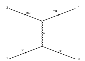
Figure 1: Born diagram relevant to the process $e\mu\to e\mu$.

As was the case for the degenerate $(n+1)$-body contribution to eq. (159), the first term on the r.h.s. of eq. (162) is non-null because the muon is massless. From eq. (I.3.27) one obtains:

$$d\hat{\sigma}_{e\mu\to e\mu}^{(C,2)}=\frac{\alpha}{2\pi}\left[-\gamma(\mu)\log\frac{\mu^{2}}{Q_{\rm ES}^{2}}+\gamma^{\prime}(\mu)-\gamma(\mu)\log\frac{s}{Q_{\rm ES}^{2}}\right]d\hat{\sigma}_{e\mu\to e\mu}^{[0]}\,.$$ (163)

Note that terms proportional to $\gamma(e)$ and $\gamma^{\prime}(e)$ are absent, since their contributions violate rule R.3. By taking eq. (160) into account, we also have:

$$d\bar{\sigma}_{e\mu\to e\mu}^{(C,2)} = d\hat{\sigma}_{e\mu\to e\mu}^{(C,2)}+\frac{\alpha}{\pi}\Bigg{[}-\gamma(\mu)\log\frac{2E_{4}}{\sqrt{s}}+C(\mu)\Bigg{(}\log\frac{2E_{2}}{\sqrt{s}}\log\frac{2E_{2}\sqrt{s}}{Q_{\rm ES}^{2}}$$ (164)

$$\phantom{aaaaaaaaa}+\log\frac{s}{Q_{\rm ES}^{2}}\log\frac{2E_{4}}{\sqrt{s}}+\log^{2}\frac{2E_{4}}{\sqrt{s}}\Bigg{)}\Bigg{]}d\hat{\sigma}_{e\mu\to e\mu}^{[0]}\,.$$

A few remarks are in order here. Firstly, terms proportional to $\gamma(e)$ and $\gamma^{\prime}(e)$ would not appear on the r.h.s. of eq. (164) even without rule R.3, because the electron is massive. Secondly, the logarithmic terms are non zero since (see eq. (153)):

$$E_{2}=E_{4}=\frac{\sqrt{s}}{2}\!\left(1-\frac{m^{2}}{s}\right)\,.$$ (165)

Thirdly, while the terms that feature $E_{4}$ can indeed be read directly from eq. (I.3.27), the one that features $E_{2}$ cannot. This is because in ref. Frederix:2018nkq it was assumed, as is customary in FKS, that both of the incoming particles are massless, and therefore that their energies are equal to $\sqrt{s}/2$. It can be easily shown that one can relax the latter condition without having to change anything in the subtraction procedure, at the price of introducing an extra term, which is the one we are discussing here. By using eq. (165) and by expanding in $m^{2}$ we finally arrive at:

$$d\bar{\sigma}_{e\mu\to e\mu}^{(C,2)}=d\hat{\sigma}_{e\mu\to e\mu}^{(C,2)}+{{\cal O}\left(\!\frac{m^{2}}{s}\!\right)}\,.$$ (166)

We now turn to the soft cross sections. Eq. (I.3.28) and rule R.3 imply that $d\hat{\sigma}_{e\mu\to e\mu}^{(S,2)}$ receives a single contribution, from the $(24)$ eikonal. The same is true for $d\bar{\sigma}_{e\mu\to e\mu}^{(S,2)}$. By taking into account eq. (160) and the fact that charged-link Borns are proportional to the Born, we obtain:

$$d\bar{\sigma}_{e\mu\to e\mu}^{(S,2)}=d\hat{\sigma}_{e\mu\to e\mu}^{(S,2)}+{{\cal O}\left(\!\frac{m^{2}}{s}\!\right)}\,.$$ (167)

Finally, owing to rule R.3 the sole virtual diagrams one must consider are those obtained by dressing the graph of fig. 1 with a triangle on the $\mu\mu\gamma$ vertex, and with a muon bubble on the $t$-channel propagator. Therefore, any electron-mass dependence may only arise when contracting the electron-line tensor with the one-loop subamplitudes (which are mass independent). Thus, no terms proportional to $\log m^{2}/s$ can possibly arise in $d\bar{\sigma}_{e\mu\to e\mu}^{(V,2)}$, which implies:

$$d\bar{\sigma}_{e\mu\to e\mu}^{(V,2)}=d\hat{\sigma}_{e\mu\to e\mu}^{(V,2)}+{{\cal O}\left(\!\frac{m^{2}}{s}\!\right)}\,.$$ (168)

From eqs. (166)–(168) we thus see that none of the $2\to 2$ cross sections contribute to eq. (148).

$\blacklozenge$ Degenerate $(n+1)$-body contribution

In the massless-electron case, there is one contribution per incoming leg (one further contribution associated with each leg is discarded because of rule R.3). Explicitly:

$$d\hat{\bar{\sigma}}_{e\mu\to e\mu(\gamma)}^{(3)}=\frac{\alpha}{2\pi}\Big{(}{\cal K}_{\gamma e}\star d\hat{\sigma}_{\gamma\mu\to\gamma\mu}^{[0]}+{\cal K}_{\mu\mu}\star d\hat{\sigma}_{e\mu\to e\mu}^{[0]}\Big{)}\,.$$ (169)

The $\star$ operator in the two terms on the r.h.s. of this equation stands for the convolution which is explicitly written in eqs. (107) and (108), respectively. The factors ${\cal K}_{\gamma e}$ and ${\cal K}_{\mu\mu}$ can be obtained from ${\cal K}_{ee}$ of eq. (109) by replacing the Altarelli-Parisi kernels and the scheme-defining function with those relevant to the branchings $e\to\gamma e$ and $\mu\to\mu\gamma$, respectively. We have:

$$P_{\mu\mu}^{<}(z) = \frac{e_{\mu}^{2}}{e_{e}^{2}}\,P_{ee}^{<}(z)\,,$$ (170)

$$P_{\mu\mu}^{\prime<}(z) = \frac{e_{\mu}^{2}}{e_{e}^{2}}\,P_{ee}^{\prime<}(z)\,,$$ (171)

and, from eq. (I.A.2):

$$P_{\gamma e}^{<}(z) = P_{ee}^{<}(1-z)=e_{e}^{2}\,\frac{1+(1-z)^{2}}{z}\,,$$ (172)

$$P_{\gamma e}^{\prime<}(z) = P_{ee}^{\prime<}(1-z)=-e_{e}^{2}\,z\,.$$ (173)

The massive-electron analogue of eq. (169) reads instead:

$$d\bar{\bar{\sigma}}_{e\mu\to e\mu(\gamma)}^{(3)}=\frac{\alpha}{2\pi}\,\bar{{\cal K}}_{\mu\mu}\star d\hat{\sigma}_{e\mu\to e\mu}^{[0]}\,,$$ (174)

the only contribution being due to the incoming massless-muon leg, and with:

$$\bar{{\cal K}}_{\mu\mu}={\cal K}_{\mu\mu}+2\log\frac{2E_{2}}{\sqrt{s}}\,\xi P_{\mu\mu}^{<}(1-\xi)\left(\frac{1}{\xi}\right)_{\!+}\,.$$ (175)

The second term on the r.h.s. of eq. (175) is due to $E_{2}$ not being equal to $\sqrt{s}/2$ (see eq. (165)), as its $2\to 2$ analogues on the r.h.s. of eq. (164). Exactly as in the $2\to 2$ case, it thus amounts to a power-suppressed term, and therefore:

$$d\bar{\bar{\sigma}}_{e\mu\to e\mu(\gamma)}^{(3)}-d\hat{\bar{\sigma}}_{e\mu\to e\mu(\gamma)}^{(3)}=-\frac{\alpha}{2\pi}\,{\cal K}_{\gamma e}\star d\hat{\sigma}_{\gamma\mu\to\gamma\mu}^{[0]}+{{\cal O}\left(\!\frac{m^{2}}{s}\!\right)}\,.$$ (176)

We finally point out that the plus distributions contained in ${\cal K}_{\gamma e}$ can be replaced with ordinary functions. In fact, the subtraction at $\xi=0$ corresponds to a soft electron and therefore is not associated with any singularity. Indeed, from the explicit expression of ${\cal K}_{\gamma e}$ we see that the residue at that point vanishes.

$\blacklozenge$ Real contributions

The diagrams that contribute to the real-emission cross sections are depicted in fig. 2. The amplitudes associated with diagrams #1 and #2 (top row) are proportional to $e_{e}e_{\mu}^{2}$, while those associated with diagrams #3 and #4 (bottom row) are proportional to $e_{e}^{2}e_{\mu}$. Therefore, owing to rule R.3, we can consider only the former two.

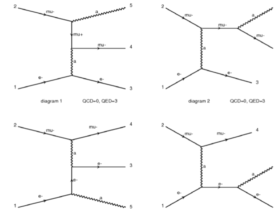
Figure 2: Real-emission diagrams relevant to the process $e\mu\to e\mu\gamma$.

The first implication of this is that the set of the FKS pairs (see e.g. ref. Frederix:2009yq ) is given by:

$${\cal P}_{\rm FKS}=\Big{\{}(5,2),(5,4),(3,1)\Big{\}}\,.$$ (177)

The sector $(5,2)$ captures soft-photon and $\mu\!\parallel\!\gamma$ initial-state collinear configurations. Likewise, the sector $(5,4)$ is associated with soft-photon and $\mu\!\parallel\!\gamma$ final-state collinear configurations. Finally, the sector $(3,1)$ singles out the $e\!\parallel\!e$ initial-state collinear configurations. Therefore, it is only the latter sector in the massive-electron case that may induce $\log m^{2}/s$ terms, or constant terms not present in the massless-electron case, since such terms emerge exclusively from quasi-collinear kinematics where potential singularities are screened by the electron mass. This implies that:

$$d\bar{\sigma}_{e\mu\to e\mu\gamma,52}^{(3)}-d\hat{\sigma}_{e\mu\to e\mu\gamma,52}^{(3)} = {{\cal O}\left(\!\frac{m^{2}}{s}\!\right)}\,,$$ (178)

$$d\bar{\sigma}_{e\mu\to e\mu\gamma,54}^{(3)}-d\hat{\sigma}_{e\mu\to e\mu\gamma,54}^{(3)} = {{\cal O}\left(\!\frac{m^{2}}{s}\!\right)}\,,$$ (179)

having denoted by $d\hat{\sigma}_{e\mu\to e\mu\gamma,ij}^{(3)}$ and $d\bar{\sigma}_{e\mu\to e\mu\gamma,ij}^{(3)}$ the contribution to $d\hat{\sigma}_{e\mu\to e\mu\gamma}^{(3)}$ and $d\bar{\sigma}_{e\mu\to e\mu\gamma}^{(3)}$, respectively, proportional to the ${\cal S}_{ij}$ function relevant to the $(i,j)$ FKS sector. One is thus left with computing the contributions due to the $(3,1)$ sector. In keeping with what was done in sect. 4.1.5, we start by considering the massive-electron case, whose cross section we write as follows:

$$d\bar{\sigma}_{e\mu\to e\mu\gamma,31}^{(3)}={\cal S}_{31}\overline{\cal M}^{(3,0)}d\bar{\phi}_{3}\,.$$ (180)

Note that since the electron is massive this FKS sector does not require any subtraction. The matrix element in eq. (180) reads as follows:

$$\overline{\cal M}^{(3,0)}=\frac{1}{4}\frac{1}{2s}\,e^{2}e_{e}^{2}\,\frac{1}{q^{4}}\,\overline{E}^{\rho\sigma}W^{\rho\sigma}\,,$$ (181)

having denoted by

$$q=\bar{p}_{1}-\bar{p}_{3}$$ (182)

the momentum flowing in the $t$-channel photon of diagrams #1 and #2 of fig. 2. The tensor associated with the $e\gamma e$ current is:

$$\overline{E}^{\rho\sigma}={\rm Tr}\Big{[}(\not{\bar{p}}_{3}-m)\gamma^{\rho}(\not{\bar{p}}_{1}-m)\gamma^{\sigma}\Big{]}=2q^{2}g^{\rho\sigma}+4\bar{p}_{1}^{\rho}\bar{p}_{3}^{\sigma}+4\bar{p}_{3}^{\rho}\bar{p}_{1}^{\sigma}\,.$$ (183)

The contribution of diagrams #1 and #2 stripped of the $e\gamma e$ current has been denoted by $W^{\rho\sigma}$, and it reads as follows:

$$W^{\rho\sigma}=\sum_{\rm pol}\Big{(}{\cal A}_{1}^{\rho\mu}+{\cal A}_{2}^{\rho\mu}\Big{)}\Big{(}{\cal A}_{1}^{\sigma\nu}+{\cal A}_{2}^{\sigma\nu}\Big{)}^{*}\left(-g^{\mu\nu}\right)\,,$$ (184)

where ${\cal A}_{i}^{\rho\mu}$ denotes the amplitude associated with the diagrams of fig. 3, with the following momenta and photon-index assignments (see eq. (150)):

$$\gamma^{\rho}(q)+\mu(p_{2})\;\longrightarrow\;\gamma^{\mu}(p_{5})+\mu(p_{4})\,.$$ (185)

Note that since $q^{2}\neq 0$, these amplitudes are off-shell.

       

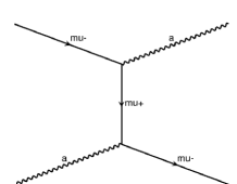
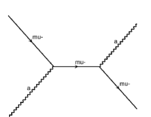
Figure 3: Diagrams relevant to the process $\gamma\mu\to\gamma\mu$. These are also the sub-graphs obtained from diagrams #1 and #2 of fig 2 by stripping them of the $e\gamma e$ current.

In eq. (184), the sum runs over the muon polarization, and the factor $-g^{\mu\nu}$ is the result of summing over the outgoing-photon polarization.

For what concerns the three-body phase space that appears in eq. (180), we decompose it as follows:

$$d\bar{\phi}_{3}=d\tilde{\phi}_{2}\,d\phi_{1}(3)\,,$$ (186)

where

$$d\tilde{\phi}_{2}=(2\pi)^{4}\delta\left(q+p_{2}-p_{4}-p_{5}\right)\frac{d^{3}p_{4}}{(2\pi)^{3}2p_{4}^{0}}\frac{d^{3}p_{5}}{(2\pi)^{3}2p_{5}^{0}}\,,$$ (187)

and, by using eq. (156):

$$d\phi_{1}(3)=\frac{d^{3}\bar{p}_{3}}{(2\pi)^{3}2\bar{p}_{3}^{0}}=\frac{1}{2(2\pi)^{3}}\,\frac{s\,\beta_{3}^{3}}{4}\,\xi d\xi\,dy\,d\varphi\,,$$ (188)

with $\varphi$ an azimuthal angle that parametrises the transverse degrees of freedom $\vec{e}$.

We now understand the integration of the r.h.s. of eq. (180) over $d\tilde{\phi}_{2}$, having fixed the variables of $d\phi_{1}(3)$. Thus, we regard the cross sections that enter eq. (148) as inclusive quantities in $d\tilde{\phi}_{2}$ which, as was anticipated, still allows us to solve that equation for $\Gamma_{\!\gamma/e}^{[1]}$. In practice, we do not need to perform such an integration explicitly. We only exploit it in the following way: at the inclusive level, the tensor $W^{\rho\sigma}$ may only depend on $q$ and $p_{2}$. Furthermore, this tensor is transverse in $q$. Therefore, we can write it in the following form:

$$W^{\rho\sigma}=T_{1}^{\rho\sigma}W_{1}+T_{2}^{\rho\sigma}W_{2}\,,$$ (189)

where

$$T_{1}^{\rho\sigma} = -g^{\rho\sigma}+\frac{q^{\rho}q^{\sigma}}{q^{2}}\,,$$ (190)

$$T_{2}^{\rho\sigma} = -\frac{q^{2}}{(p_{2}\!\cdot\!q)^{2}}\,\left(p_{2}^{\rho}-\frac{p_{2}\!\cdot\!q}{q^{2}}q^{\rho}\right)\left(p_{2}^{\sigma}-\frac{p_{2}\!\cdot\!q}{q^{2}}q^{\sigma}\right)\,,$$ (191)

and the scalar functions $W_{i}$ depend only on $q^{2}$ and $p_{2}\!\cdot\!q$. Given $W^{\rho\sigma}$ (e.g. as computed from amplitudes like those on the r.h.s. of eq. (184)), these functions can be projected out as follows:

$$W_{1} = -\frac{1}{2}\left(g^{\rho\sigma}+\frac{q^{2}}{(p_{2}\!\cdot\!q)^{2}}\,p_{2}^{\rho}p_{2}^{\sigma}\right)W^{\rho\sigma}\,,$$ (192)

$$W_{2} = -\frac{1}{2}\left(g^{\rho\sigma}+3\,\frac{q^{2}}{(p_{2}\!\cdot\!q)^{2}}\,p_{2}^{\rho}p_{2}^{\sigma}\right)W^{\rho\sigma}\,.$$ (193)

By using the decomposition of eq. (189) in eq. (181), we see that two relevant quantities are:

$$\overline{E}^{\rho\sigma}T_{1}^{\rho\sigma} = -4\left(q^{2}+2m^{2}\right)\,,$$ (194)

$$\overline{E}^{\rho\sigma}T_{2}^{\rho\sigma} = -8q^{2}\frac{F}{(1-F)^{2}}\,,$$ (195)

where

$$F=\frac{1}{2}\,\xi\left(1+\beta_{3}y\right)\,.$$ (196)

Therefore:

$$\overline{\cal M}^{(3,0)}=-\frac{1}{4}\frac{1}{2s}\,e^{2}e_{e}^{2}\,\frac{1}{q^{4}}\left[4\left(q^{2}+2m^{2}\right)W_{1}+8q^{2}\frac{F}{(1-F)^{2}}\,W_{2}\right]\,.$$ (197)

Now observe that:

$$p_{2}\!\cdot\!q = \frac{1}{2}\,(s-m^{2})\,(1-F)\,,$$ (198)

$$q^{2} = -\frac{s}{2}\left[\xi\left(1+\frac{m^{2}}{s}\right)-\frac{4m^{2}}{s}\right]\left(1-\frac{y}{1+\rho}\right)\,,$$ (199)

where

$$\rho=\frac{\xi(1-\beta_{3})-(4-\xi(1+\beta_{3}))m^{2}/s}{\xi\beta_{3}(1-m^{2}/s)}=2\,\frac{(1-\xi)^{2}}{\xi^{2}}\,\frac{m^{2}}{s}+{\cal O}\left(\frac{m^{4}}{s^{2}}\right)\,.$$ (200)

In the collinear ($y\to 1$) and massless-electron limit, we have $q^{2}\to 0$ as expected, and $p_{2}\!\cdot\!q\to s(1-\xi)/2$. Therefore, by regarding the r.h.s. of eq. (197) as an expansion in $q^{2}$, the dominant terms in the collinear limit will be proportional to $1/q^{4}$ and $1/q^{2}$. However, one must not exclude the possibility that either (or both) of the residue(s) of these terms is (are) equal to zero. In order to check this, we must study the behaviour of the $W_{i}$ functions in the $q^{2}\to 0$ limit. By means of an explicit computation we obtain what follows:

$$W_{1}=W_{2}=\frac{1}{2}B_{\gamma\mu\to\gamma\mu}+{\cal O}(q^{2})\,,$$ (201)

where $B_{\gamma\mu\to\gamma\mu}$ is the matrix element squared and summed over all polarisations of the process $\gamma\mu\to\gamma\mu$. The momenta are assigned as in eq. (185) with $q^{2}=0$, which implies $q=(1-\xi)p_{1}$. In other words:

$${\cal M}^{(2,0)}_{\gamma\mu\to\gamma\mu}\big{(}(1-\xi)p_{1},p_{2}\big{)}=\frac{1}{4}\,\frac{1}{2(1-\xi)s}\,B_{\gamma\mu\to\gamma\mu}\,.$$ (202)

Equation (201) implies that both the $1/q^{4}$ and the $1/q^{2}$ appear non-trivially in eq. (197). By using the expression of $q^{2}$ given in eq. (199), the former term is dealt with by means of the identity of eq. (129). As far as the $1/q^{2}$ term is concerned, another distribution identity is necessary, namely:

$$\frac{1}{1-\frac{y}{1+\rho}}=-\log\frac{\rho}{2}\,\,\delta(1-y)+\left(\frac{1}{1-y}\right)_{\!+}+{\cal O}(\rho)\,.$$ (203)

After employing eqs. (129) and (203) in eq. (197), one can safely set $m=0$ in the latter. The resulting cross section of eq. (180) is the sum of two terms: one proportional to $\delta(1-y)$, and one proportional to $1/(1-y)_{+}$. It is easy to see that the latter is nothing but the real-emission contribution of the $(3,1)$ FKS sector to the massless-electron cross section. The former term must be explicitly computed, which is straightforward owing to the simplifications induced by $\delta(1-y)$. In particular, such a $\delta$ will allow us to use eq. (201) with all of the ${\cal O}(q^{2})$ terms identically equal to zero; in other words, the quantity on the l.h.s. of eq. (202) will naturally emerge. We also have:

$$\delta(1-y)\,d\tilde{\phi}_{2} = \delta(1-y)\,d\phi_{2}\big{(}(1-\xi)s\big{)}\,,$$ (204)

$$\delta(1-y)\,F = \delta(1-y)\,\xi+{{\cal O}\left(\!\frac{m^{2}}{s}\!\right)}\,,$$ (205)

$$\delta(1-y)\,{\cal S}_{31} = \delta(1-y)\,,$$ (206)

where the $d\phi_{2}$ on the r.h.s. of eq. (204) is the two-body massless phase space with incoming energy squared equal to $(1-\xi)s$. By putting all this together, some trivial algebra leads us to the final result:

$$d\bar{\sigma}_{e\mu\to e\mu\gamma,31}^{(3)}-d\hat{\sigma}_{e\mu\to e\mu\gamma,31}^{(3)}=\frac{\alpha}{2\pi}\,{\cal Q}_{\gamma e}\star d\hat{\sigma}_{\gamma\mu\to\gamma\mu}^{[0]}+{{\cal O}\left(\!\frac{m^{2}}{s}\!\right)}\,,$$ (207)

where

$${\cal Q}_{\gamma e}(1-\xi)=-e_{e}^{2}\left[\frac{1+\xi^{2}}{1-\xi}\left(2\log\frac{1-\xi}{\xi}+\log\frac{m^{2}}{s}\right)+\frac{2\xi}{1-\xi}\right]\,.$$ (208)

4.2.3 Final result

We can now use eqs. (166), (167), (168), (176), (178), (179), and (207) in eq. (148). We obtain:

$$\Gamma_{\!\gamma/e}^{[1]}(z)=-{\cal K}_{\gamma e}(z)+{\cal Q}_{\gamma e}(z)\,.$$ (209)

Therefore:

$$\Gamma_{\!\gamma/e}^{[1]}(z,\mu^{2})=e_{e}^{2}\,\frac{1+(1-z)^{2}}{z}\left(\log\frac{\mu^{2}}{m^{2}}-2\log z-1\right)+e_{e}^{2}K_{\gamma e}(z)\,.$$ (210)

By comparing this result with that of eq. (142), we see that:

$$\Gamma_{\!\gamma/e}^{[1]}(z)-e_{e}^{2}K_{\gamma e}(z)=\Gamma_{\!e/e}^{[1]}(1-z)-e_{e}^{2}K_{ee}(1-z)\,,\;\;\;\;\;\;\;\;z<1\,.$$ (211)

We thus find that the $z\to 1-z$ symmetry property characteristic of the unsubtracted Altarelli-Parisi kernels $P_{ee}$ and $P_{\gamma e}$ also holds for the unsubtracted QED PDFs at ${\cal O}(\alpha)$, up to scheme-change terms. This is nicely consistent with the idea of collinear factorisation. It would be tempting to conclude that it is also an indication that:

$$K_{\gamma e}(z)=K_{ee}(1-z)\,,\;\;\;\;\;\;\;\;z<1\,.$$ (212)

While eq. (212) constitutes a valid choice (in particular, it is trivially true in $\overline{\rm MS}$), the current computation cannot possibly suggest that it is the only suitable choice.

We finally point out that the procedure followed above implies that the quantity:

$$\frac{\alpha}{2\pi}\,{\cal Q}_{\gamma e}(z)=e_{e}^{2}\,\frac{\alpha}{2\pi}\,\left[\frac{1+(1-z)^{2}}{z}\log\frac{(1-z)^{2}s}{z^{2}m^{2}}-\frac{2(1-z)}{z}\right]$$ (213)

is the kernel that collects all universal (i.e. independent of the process and of the subtraction scheme) purely collinear terms of the $e(1)\to\gamma(z)e(1-z)$ splitting. As such, it must be equivalent to the Weizsaecker-Williams (WW) function. This is indeed the case: eq. (213) coincides e.g. with eq. (27) of ref. Frixione:1993yw , provided that in the latter: a) one identifies $E^{2}\theta_{c}^{2}$ with $s$ (which can be understood from the physical viewpoint by noting that $E^{2}\theta_{c}^{2}$ is the “large” scale of the problem); b) one neglects all terms which are suppressed by powers of $m^{2}$ (some of these have been kept in ref. Frixione:1993yw , while they are strictly discarded here). Equation (209) thus clarifies the relationship between the WW function and $\Gamma_{\!\gamma/e}^{[1]}(z)$, which do not coincide (as is clear in general from the fact that the PDF depends on an arbitrary mass scale ($\mu$) and is defined in an arbitrary scheme).

5 Initial conditions for PDFs through collinear factorisation

The results obtained in sects. 4.1 and 4.2 have, among other things, three key properties, which we now enumerate. One of these will provide a way to compute the PDFs in an alternative and simpler way w.r.t. what was done so far (namely through collinear-factorisation properties), thus allowing a quick determination of the photon PDFs, $\Gamma_{\!e/\gamma}$ and $\Gamma_{\!\gamma/\gamma}$.

$\bullet$ Consistency with evolution equations. Electron and photon PDFs must obey the DGLAP equations (9). By employing eqs. (10) and (15), in the case of the electron PDFs eq. (9) reads:

$$\frac{\partial\Gamma_{\!i/e}^{[1]}}{\partial\log\mu^{2}}=P_{ie}^{[0]}\,,$$ (214)

where we have added (w.r.t. to the notation used in the rest of this paper) an index $[0]$ to the lowest-order splitting kernel, in order to avoid confusions. Equation (214) is manifestly fulfilled by $\Gamma_{\!e/e}^{[1]}$ of eq. (142) and by $\Gamma_{\!\gamma/e}^{[1]}$ of eq. (210) – note that the scheme-change terms must be, by construction, independent of $\mu$. In the case of the photon PDFs, eq. (9) leads to:

$$\frac{\partial\Gamma_{\!i/\gamma}^{[1]}}{\partial\log\mu^{2}}=P_{i\gamma}^{[0]}\,.$$ (215)

$\bullet$ Momentum and charge conservation. In pure QED, the condition of momentum conservation in the branchings of a fermion $f^{\pm}$ with electric charge $\pm 1$ reads, in terms of its PDFs (by ignoring other fermion families):

$$1=\int_{0}^{1}dz\,z\Big{(}\Gamma_{\!f^{\pm}/f^{\pm}}(z)+\Gamma_{\!\gamma/f^{\pm}}(z)+\Gamma_{\!f^{\mp}/f^{\pm}}(z)\Big{)}\,.$$ (216)

By taking $f$ to be an electron or a positron and by using eq. (15), at the first non-trivial order in $\alpha$ eq. (216) becomes:

$$0=\int_{0}^{1}dz\,z\Big{(}\Gamma_{\!e/e}^{[1]}(z)+\Gamma_{\!\gamma/e}^{[1]}(z)\Big{)}\,.$$ (217)

With the explicit results of eqs. (142) and (210) we can verify that the terms not related to the change of scheme fulfill eq. (217), and therefore that the latter can be turned into a condition that the scheme-change terms must fulfill as well:

$$\int_{0}^{1}dz\,z\Big{(}K_{ee}(z)+K_{\gamma e}(z)\Big{)}=0\,.$$ (218)

The analogue of eq. (216) for the branchings of a photon reads:

$$1=\int_{0}^{1}dz\,z\Big{(}\Gamma_{\!\gamma/\gamma}(z)+\Gamma_{\!f^{+}/\gamma}(z)+\Gamma_{\!f^{-}/\gamma}(z)\Big{)}\,.$$ (219)

By taking eq. (15) into account, and by considering only the lightest lepton family as representative of charged fermions, at the first non-trivial order in $\alpha$ eq. (219) becomes:

$$0=\int_{0}^{1}dz\,z\Big{(}\Gamma_{\!\gamma/\gamma}^{[1]}(z)+2\Gamma_{\!e/\gamma}^{[1]}(z)\Big{)}\,.$$ (220)

Finally, with the same assumptions as for eq. (216), the charge-conservation condition for $f^{\pm}$ reads:

$$1=\int_{0}^{1}dz\,\Big{(}\Gamma_{\!f^{\pm}/f^{\pm}}(z)-\Gamma_{\!f^{\mp}/f^{\pm}}(z)\Big{)}\,.$$ (221)

For the electron at ${\cal O}(\alpha)$ and again thanks to eq. (15), this implies:

$$0=\int_{0}^{1}dz\,\Gamma_{\!e/e}^{[1]}(z)\,,$$ (222)

which can be seen immediately to be fulfilled (possibly bar for the scheme-change term) by eq. (142). Therefore, in analogy to eq. (217), eq. (222) can be used to impose a constraint of the $\Gamma_{\!e/e}$ scheme-change term:

$$\int_{0}^{1}dz\,K_{ee}(z)=0\,.$$ (223)

$\bullet$ What determines the PDFs. As far as the contributions to $\Gamma_{\!i/e}^{[1]}(z)$ are concerned, the computations of sects. 4.1 and 4.2 show that they originate from the following three different sources.

1. For $z<1$, the difference between the real-emission massive-electron cross section, and its massless-electron counterpart. Crucially, such a difference leads to logarithmically-enhanced and/or constant terms in the electron mass only in the kinematics region dominated by the collinear splittings of the incoming electron.

2. For $z<1$, the contribution to the $(n+1)$-body degenerate cross section due to the incoming electron leg.

3. For $z=1$, the soft-subtraction terms of the two contributions above, plus the differences between the massive- and massless-electron cross sections for all of the Born-like cross sections.

This suggests an alternative procedure for the determination of the PDFs. Let us first deal with the case of $\Gamma_{\!e/e}^{[1]}$ to be definite. Consider the $(n+1)$-body process:

$$e+x_{2}\;\longrightarrow x_{3}+\ldots x_{n+2}+\gamma\,,$$ (224)

with $x_{i}$ being particles/partons whose nature is unimportant here, and its $n$-body counterpart:

$$e+x_{2}\;\longrightarrow x_{3}+\ldots x_{n+2}\,.$$ (225)

The master equation to be solved for $\Gamma_{\!e/e}^{[1]}(z)$ for $z<1$ is:

$$d\bar{\sigma}^{(n+1)}-d\hat{\sigma}^{(n+1)}-d\hat{\bar{\sigma}}^{(n+1)}=\frac{\alpha}{2\pi}\,\Gamma_{\!e/e}^{[1]}\star d\hat{\sigma}^{(n)}\,.$$ (226)

With abuse of notation, we have written the real-emission and degenerate cross sections in eq. (226) as if they were the exact ones, but we actually mean to use simplified forms in keeping with items 1 and 2 above. As far as the real-emissions contribution is concerned, we shall employ:

$$d\bar{\sigma}^{(n+1)} = {\cal S}_{n+3,1}\overline{\cal M}^{(n+1,0)}d\phi_{n+1}\,,$$ (227)

$$\overline{\cal M}^{(n+1,0)} = \frac{2e^{2}}{(k_{1}-k_{n+3})^{2}-m^{2}}\,P_{e^{\star}e}^{<}\left(z\right)\,{\cal M}^{(n,0)}(zk_{1})\,.$$ (228)

We have labelled the outgoing photon with index $n+3$; thus, the ${\cal S}$ function ${\cal S}_{n+3,1}$ selects kinematic configurations where the photon is collinear to the incoming electron. Furthermore, the real-emission matrix element of eq. (228), relevant to the process of eq. (224), is taken equal to its collinear limits, computed according to the procedure outlined in appendix B (see in particular eq. (327)). The $n$-body matrix element on the r.h.s. of eq. (228) is the one relevant to the process of eq. (225). Finally, the absence of soft subtractions in eq. (227) is due to the fact that the solution obtained from eq. (226) is valid only for $z<1$. As far as the degenerate cross section is concerned, following item 2 we need to consider only the contribution due to emissions from leg 1. Thus, from eq. (107) we obtain:

$$d\hat{\bar{\sigma}}^{(n+1)} = \frac{\alpha}{2\pi}\,{\cal K}_{ee}\star d\hat{\sigma}^{(n)}\,,$$ (229)

$$d\hat{\sigma}^{(n)} = {\cal M}^{(n,0)}d\phi_{n}\,,$$ (230)

and ${\cal K}_{ee}$ given in eq. (109) (without the plus prescriptions).

Given these cross sections, the idea is the following. Since the leading behaviour for $m\to 0$ of the real-emission cross section results from integrating over collinear photon-electron configurations, the relevant kinematics quantities are explicitly given in the prefactor on the r.h.s. of eq. (228). The integration itself is then performed, trivially, by means of identities such as those of eqs. (128), (129), and (203). These do not allow one to obtain $d\bar{\sigma}^{(n+1)}$, but rather the difference $d\bar{\sigma}^{(n+1)}-d\hat{\sigma}^{(n+1)}$, which however is the only thing that matters given eq. (226). In the process, we expect $d\hat{\sigma}^{(n)}$ to factorise.

Having done this, the solution at $z=1$ is obtained by using either the momentum- or the charge-conservation condition. The consistency with evolution equations could be used as well, but it turns out not to be necessary. We point out that momentum conservation requires one to solve first for both $\Gamma_{\!e/e}^{[1]}$ and $\Gamma_{\!\gamma/e}^{[1]}$ for $z<1$. This is feasible, since it should be clear that the procedure outlined above can in fact be applied to any kind of splittings (including those in which it is an initial-state photon that splits), with only trivial modifications to eqs. (226), (228), and (229).

$\bullet$ Relationships with QCD results. The previous item renders it clear that there are strict similarities between the PDFs which are computed here, and the so-called parton-to-parton (p2p henceforth) PDFs which emerge in the context of factorisation theorems in QCD; the same remark applies to fragmentation functions (FFs) as well. One must keep in mind that while the electron and photon QED PDFs and FFs are directly connected with physical cross sections, their p2p QCD counterparts enter unphysical factorisation formulae, whose connections with observable quantities always imply the introduction of long-distance objects (the proper hadronic PDFs and FFs). With this observation in mind, and provided that one relies on QCD factorisation formulae written in the same way as eq. (21), one can obtain the QED PDFs and FFs from their p2p QCD analogues by taking the abelian limit of the latter; furthermore, the p2p PDFs and FFs must have been computed with one massive flavour (which in the abelian limit will play the role of the electron in QED); the contributions of the massless flavours must be discarded.

The previous conditions imply that, with the exception of final-state $b$ quarks (for the reasons explained in footnote 10), the QCD results we are interested in are those generally called “variable flavour number scheme” approaches, in which one studies the cross sections where one massive flavour (typically, the $b$ quark) undergoes a transition from a kinematical regime where its mass is not negligible to another regime where it can be treated as if it were massless. As far as the initial-state case (i.e. the PDFs) is concerned, the first NLO results can be found in ref. Aivazis:1993pi (see e.g. ref. Olness:1997yc for their explicit applications to cross section computations). We must note that these results do not include the case of the $b$-to-$b$ PDF (i.e. the analogue of $\Gamma_{\!e/e}$ computed here), since this would require the assumption of an intrinsic $b$-quark hadronic component, which is typically not made. Such a quantity has been computed in the context of DIS in ref. Kretzer:1998ju . Conversely, the final-state case (i.e. the FFs) has been considered in ref. Mele:1990cw ($b$-to-$b$, on which we shall further comment in sect. 6.2) and in ref. Cacciari:2005ry (the other flavours). We also point out that the QED $e$-to-$\gamma$ FF has several analogies with the (massive) quark-to-$\gamma$ FF, computed at the NLO in QCD in ref. Glover:1993xc (we shall briefly return on this point in sect. 6.3).

We conclude this discussion with two observations. Firstly, the QCD results are generally derived in the $\overline{\rm MS}$ scheme. In QED, it is convenient to be able to exploit the flexibility associated with changing the subtraction scheme – we shall show this explicitly in ref. BCCFS and subsequent publications. Secondly, having established at the NLO the close relationships between the QED PDFs and FFs as computed here and their p2p QCD counterparts, it appears safe to assume that these will hold true also at orders higher than NLO. Thus, one could exploit the (N)NLO computations of refs. Buza:1995ie ; Buza:1996wv ; Blumlein:2018jfm (initial state) and refs. Melnikov:2004bm ; Mitov:2004du (final state).

5.1 Kinematics

We parametrise the momenta of the partons involved in the splitting of interest as follows:

$$k_{1} = \frac{\sqrt{s}}{2}(1,0,0,\beta_{1})$$ (231)

$$k_{n+3} = \frac{\sqrt{s}}{2}\,\xi\left(1,\vec{e}\,\sqrt{1-y^{2}}\,\beta_{n+3},y\,\beta_{n+3}\right)\,,$$ (232)

with $k_{i}$ the momentum of parton $i$ (as e.g. in eq. (224)), $s=(k_{1}+k_{2})^{2}$ and:

$$\beta_{1}=\sqrt{1-\frac{4m_{1}^{2}}{s}}\,,\;\;\;\;\;\;\;\;\beta_{n+3}=\sqrt{1-\frac{4m_{n+3}^{2}}{s\,\xi^{2}}}\,.$$ (233)

As usual, we identify $\xi=1-z$, $z$ being that which appears in eq. (228). The masses $m_{1}$ and $m_{n+3}$ can be either equal to the electron mass $m$ or to zero, depending on the type of branching being studied. We point out the following fact. The expression of the momentum of the incoming parton in eq. (231) is the same as that in eq. (25), but differs from that in eq. (152). The difference in the latter two forms is due to the fact that the FKS cross sections are written in the incoming partons c.m. frame, hence the parametrisation of the momentum of parton 1 depends (also) on the mass of parton 2. By employing eq. (231), we have assumed that the mass of parton 2 is equal to $m_{1}$. This might appear odd, since parton 2 never appears in the procedure advocated in this section for the extraction of the PDFs. In fact, such choices do not have an impact on the final results, and are made with the sole purpose of simplifying the computation. This is because the PDF we seek to calculate is a purely collinear quantity, and hence is invariant under longitudinal boosts. Therefore, computations carried out in any two frames connected by longitudinal boosts will necessarily lead to the same PDFs. An a posteriori evidence in support of this argument is the fact that we shall obtain here the same result for $\Gamma_{\!\gamma/e}^{[1]}$ as in eq. (210), in spite of the difference between eq. (231) and eq. (152).

The $(n+1)$-body phase-space is:

$$d\phi_{n+1}(k_{1},\ldots k_{n+3}) = d\tilde{\phi}_{n}(k_{1},\ldots k_{n+3})\,d\phi_{1}(k_{n+3})\,,$$ (234)

$$d\tilde{\phi}_{n}(k_{1},\ldots k_{n+3}) = (2\pi)^{4}\delta\left(k_{1}+k_{2}-\sum_{i=3}^{n+3}k_{i}\right)\prod_{i=3}^{n+2}\frac{d^{3}k_{i}}{(2\pi)^{3}2k_{i}^{0}}\,,\phantom{aaa}$$ (235)

$$d\phi_{1}(k_{n+3}) = \frac{d^{3}k_{n+3}}{(2\pi)^{3}2k_{n+3}^{0}}=\frac{1}{2(2\pi)^{3}}\,\frac{s\beta_{n+3}^{3}}{4}\,\xi d\xi\,dy\,d\varphi\,.$$ (236)

For future use, we note the property:

$$d\tilde{\phi}_{n}(k_{1},\ldots k_{n+3})\,\delta(1-y)\;\stackrel{{\scriptstyle m_{1}\to 0\,,m_{n+3}\to 0}}{{\longrightarrow}}\;d\phi_{n}\big{(}(1-\xi)k_{1},\ldots k_{n+2}\big{)}\,\delta(1-y)\,.$$ (237)

The leftmost quantity on the r.h.s. of eq. (237) is the actual $n$-body phase-space with incoming massless legs and incoming energy squared equal to $(1-\xi)s$.

5.2 Determination of $\Gamma_{\!e/e}$

In this case, the relevant branching is $e\to e^{\star}\gamma$, whence $m_{1}=m$ and $m_{n+3}=0$. With the QED version of eq. (328), eq. (227) becomes:

$$d\bar{\sigma}^{(n+1)} = {\cal S}_{n+3,1}e^{2}e_{e}^{2}\left[\frac{1}{k_{1}\!\cdot\!k_{n+3}}\,\frac{1+(1-\xi)^{2}}{\xi}-\frac{(1-\xi)m^{2}}{\big{(}k_{1}\!\cdot\!k_{n+3}\big{)}^{2}}\right]$$ (238)

$$\times {\cal M}^{(n,0)}\big{(}(1-\xi)k_{1}\big{)}\,\frac{s}{8(2\pi)^{3}}\,\xi d\xi dyd\varphi d\tilde{\phi}_{n}\,.$$

With eqs. (231) and (232):

$$k_{1}\!\cdot\!k_{n+3}=\frac{s}{4}\,\xi\left(1-\beta_{1}y\right)\equiv\frac{s}{4}\,\xi\left(1-\frac{y}{1+\rho}\right)\,,$$ (239)

where as was done in eq. (130) we have defined:

$$\rho=\frac{1-\beta_{1}}{\beta_{1}}=2\,\frac{m^{2}}{s}+{\cal O}\left(\!\frac{m^{4}}{s^{2}}\!\right)\,.$$ (240)

One can then replace eq. (239) into eq. (238), and employ the identities in eqs. (203) and (129) for the first and second term in the square brackets, respectively, which also allows one to set equal to zero all mass terms that are not explicitly written in eq. (238) and in $\rho$. By doing so, a number of things follow. Firstly, the plus-distribution contribution of eq. (203) results in the collinearly-subtracted massless-electron cross section $d\hat{\sigma}^{(n+1)}$. All of the remaining contributions are then proportional to $\delta(1-y)$, and one can exploit:

$${\cal S}_{n+3,1}\delta(1-y)=\delta(1-y)\,,$$ (241)

and eq. (237). From this and from the matrix element on the r.h.s. of eq. (238), the reduced cross section of eq. (230) (evaluated at the reduced c.m. energy $(1-\xi)s$) emerges naturally. By performing the trivial $y$ and $\varphi$ integrations we finally obtain:

$$d\bar{\sigma}^{(n+1)} = d\hat{\sigma}^{(n+1)}+\frac{\alpha}{2\pi}\,e_{e}^{2}\left[\frac{1+(1-\xi)^{2}}{\xi}\log\frac{s}{m^{2}}-2\,\frac{1-\xi}{\xi}\right]$$ (242)

$$\phantom{d\hat{\sigma}^{(n+1)}+\frac{\alpha}{2\pi}\,e_{e}^{2}}\times d\hat{\sigma}^{(n)}\big{(}(1-\xi)k_{1}\big{)}\,d\xi\,.$$

We can now replace this result into our master equation (226). By using there the explicit expression of the degenerate cross section, by identifying $\xi$ with $1-z$, and by solving for $\Gamma_{\!e/e}^{[1]}(z)$, we obtain again eq. (142), with the exception of the plus prescription (since we have worked here with $z<1$). However, the contribution at $z=1$ can be readily obtained by exploiting the charge-conservation condition of eq. (222).

As a final technical aside, we point out that, in order to obtain the third term in the round brackets of eq. (142) with the procedure we have followed here, the factor $1-\xi$ in the numerator of the second term in the square brackets of eq. (238) is crucial. In turn, this is a direct consequence of the crossing we have employed in app. B to determine the massive spacelike splitting kernels.

5.3 Determination of $\Gamma_{\!\gamma/e}$

In this case, the relevant branching is $e\to\gamma^{\star}e$, whence $m_{1}=m$ and $m_{n+3}=m$. With the QED version of eq. (329), eq. (227) becomes:

$$d\bar{\sigma}^{(n+1)} = {\cal S}_{n+3,1}e^{2}e_{e}^{2}\left[\frac{1}{k_{1}\!\cdot\!k_{n+3}-m^{2}}\,\frac{1+\xi^{2}}{1-\xi}-\frac{(1-\xi)m^{2}}{\big{(}k_{1}\!\cdot\!k_{n+3}-m^{2}\big{)}^{2}}\right]$$ (243)

$$\times {\cal M}^{(n,0)}\big{(}(1-\xi)k_{1}\big{)}\,\frac{s}{8(2\pi)^{3}}\,\beta_{n+3}^{3}\,\xi d\xi dyd\varphi d\tilde{\phi}_{n}\,.$$

The analogue of eq. (239) reads:

$$k_{1}\!\cdot\!k_{n+3}-m^{2}=\frac{s}{4}\left(\xi-\frac{4m^{2}}{s}\right)\left(1-\frac{y}{1+\rho}\right)\,,$$ (244)

having defined

$$\rho=\frac{\xi(1-\beta_{1}\beta_{n+3})-4m^{2}/s}{\xi\beta_{1}\beta_{n+3}}=2\,\frac{(1-\xi)^{2}}{\xi^{2}}\,\frac{m^{2}}{s}+{\cal O}\left(\!\frac{m^{4}}{s^{2}}\!\right)\,.$$ (245)

We can now perform the same algebraic operations already carried out in sect. 5.2, to obtain what follows:

$$d\bar{\sigma}^{(n+1)}=d\hat{\sigma}^{(n+1)}+\frac{\alpha}{2\pi}\,{\cal Q}_{\gamma e}\star d\hat{\sigma}^{(n)}\,,$$ (246)

namely, the very same result as in eq. (207). This implies that we also obtain again the final result for $\Gamma_{\!\gamma/e}^{[1]}$ already reported in eq. (210).

5.4 Determination of $\Gamma_{\!e/\gamma}$

In this case, the relevant branching is $\gamma\to e^{\star}e$, whence $m_{1}=0$ and $m_{n+3}=m$. With the QED version of eq. (330), eq. (227) becomes:

$$d\bar{\sigma}^{(n+1)} = {\cal S}_{n+3,1}e^{2}e_{e}^{2}\left[\frac{(1-\xi)^{2}+\xi^{2}}{k_{1}\!\cdot\!k_{n+3}}+\frac{(1-\xi)m^{2}}{\big{(}k_{1}\!\cdot\!k_{n+3}\big{)}^{2}}\right]$$ (247)

$$\times {\cal M}^{(n,0)}\big{(}(1-\xi)k_{1}\big{)}\,\frac{s}{8(2\pi)^{3}}\,\beta_{n+3}^{3}\,\xi d\xi dyd\varphi d\tilde{\phi}_{n}\,.$$

The analogue of eq. (239) reads:

$$k_{1}\!\cdot\!k_{n+3}=\frac{s}{4}\,\xi\left(1-\beta_{n+3}y\right)\equiv\frac{s}{4}\,\xi\left(1-\frac{y}{1+\rho}\right)\,,$$ (248)

with:

$$\rho=\frac{1-\beta_{n+3}}{\beta_{n+3}}=\frac{2}{\xi^{2}}\,\frac{m^{2}}{s}+{\cal O}\left(\!\frac{m^{4}}{s^{2}}\!\right)\,.$$ (249)

A simple algebra leads one to:

$$d\bar{\sigma}^{(n+1)} = d\hat{\sigma}^{(n+1)}+\frac{\alpha}{2\pi}\,e_{e}^{2}\left[\left(\xi^{2}+(1-\xi)^{2}\right)\log\frac{s\xi^{2}}{m^{2}}+2\xi(1-\xi)\right]$$ (250)

$$\phantom{d\hat{\sigma}^{(n+1)}+\frac{\alpha}{2\pi}\,e_{e}^{2}}\times d\hat{\sigma}^{(n)}\big{(}(1-\xi)k_{1}\big{)}\,d\xi\,.$$

The relevant $(n+1)$-body degenerate cross section is:

$$d\hat{\bar{\sigma}}^{(n+1)} = \frac{\alpha}{2\pi}\,{\cal K}_{e\gamma}\star d\hat{\sigma}^{(n)}\,,$$ (251)

$${\cal K}_{e\gamma}(z) = P_{e\gamma}^{<}(z)\left(\log\frac{s}{\mu^{2}}+2\log(1-z)\right)-P_{e\gamma}^{\prime<}(z)-e_{e}^{2}K_{e\gamma}(z)\,.\phantom{aaa}$$ (252)

By using:

$$P_{e\gamma}^{<}(z) = e_{e}^{2}\left(z^{2}+(1-z)^{2}\right)\,,$$ (253)

$$P_{e\gamma}^{\prime<}(z) = -e_{e}^{2}z(1-z)\,,$$ (254)

we finally obtain:

$$\Gamma_{\!e/\gamma}^{[1]}(z,\mu^{2})=e_{e}^{2}\left(z^{2}+(1-z)^{2}\right)\log\frac{\mu^{2}}{m^{2}}+e_{e}^{2}K_{e\gamma}(z)\,.$$ (255)

This result fulfills eq. (215), as expected. Note that it is also valid at $z=1$, since the branching $\gamma\to e^{\star}e$ cannot induce soft singularities.

5.5 Determination of $\Gamma_{\!\gamma/\gamma}$

The absence of a $\gamma\to\gamma X$ splitting at ${\cal O}(\alpha)$ implies that all of the cross sections on the l.h.s. of eq. (226) are identically equal to zero. This implies that the photon-to-photon PDF must have the following form:

$$\Gamma_{\!\gamma/\gamma}^{[1]}(z,\mu^{2})=\left(A\log\frac{\mu^{2}}{m^{2}}+B\right)\delta(1-z)\,.$$ (256)

Neglecting the scheme-change term in eq. (255) for the time being, eq. (220) implies:

$$A\log\frac{\mu^{2}}{m^{2}}+B+2e_{e}^{2}\log\frac{\mu^{2}}{m^{2}}\int_{0}^{1}dz\,z\left(z^{2}+(1-z)^{2}\right)=0\,.$$ (257)

By solving for $A$ and $B$ one obtains:

$$A = -\frac{2}{3}e_{e}^{2}\,,$$ (258)

$$B = 0\,.$$ (259)

By introducing an arbitrary change-of-scheme function, the photon PDFs then reads:

$$\Gamma_{\!\gamma/\gamma}^{[1]}(z,\mu^{2})=-\frac{2}{3}e_{e}^{2}\log\frac{\mu^{2}}{m^{2}}\,\delta(1-z)+e_{e}^{2}K_{\gamma\gamma}(z)\,,$$ (260)

where, analogously to eq. (218):

$$\int_{0}^{1}dz\,z\Big{(}K_{e\gamma}(z)+K_{\gamma\gamma}(z)\Big{)}=0\,.$$ (261)

The result of eq. (260), which can be immediately extended to the case of several massive charged fermions, fulfills eq. (215).

6 Initial conditions for fragmentation functions

What has been done in sect. 5 can also be applied to the case in which one considers final-state, rather than initial-state, branchings. There, it is one of the outgoing partons whose momentum becomes constrained by the object that plays the same role as the one played by the PDFs so far – namely, the fragmentation function (FF). The FKS formalism has been extended to include FFs in ref. Frederix:2018nkq ; the formulae are given in that paper for QCD, but it is immediate to covert them into their QED counterparts, which is what we are interested in here, by means of eqs. (319) and (320).

We shall write the cross section for the production of a particle $H$ as follows:

$$d\sigma_{H}=\sum_{p}d\hat{\sigma}_{p}\star D_{\!H/p}\,,$$ (262)

whose explicit definition can be found in ref. Frederix:2018nkq . We shall employ eq. (262) up to the first non-trivial order in $\alpha$ with:

$$p,\,H\;\in\;\{e^{+},e^{-},\gamma\}\,.$$ (263)

The notation of eq. (262) understands that:

$$D_{\!H/p}\,:\;\;\;\;\;\;\;\;p\,\stackrel{{\scriptstyle\rm fragments}}{{\longrightarrow}}\,H\,.$$ (264)

In QED, the FFs admit a perturbative expansion:

$$D_{\!H/p}(z)=D_{\!H/p}^{[0]}(z)+\frac{\alpha}{2\pi}\,D_{\!H/p}^{[1]}(z)+{\cal O}(\alpha^{2})\,,$$ (265)

where, analogously to eq. (15), we must have:

$$D_{\!H/p}^{[0]}(z,\mu^{2})=\delta_{Hp}\,\delta(1-z)\,.$$ (266)

The basic idea behind eq. (262) is the following: compute the particle cross section on the l.h.s. with massive electrons, and keep the dominant terms as $m\to 0$; compute the subtracted partonic cross sections on the r.h.s. with massless electrons; and solve for $D_{\!H/p}(z)$. By performing this procedure in the context of complete-process computations one is conceptually on the very same footing as in sects. 4.1 and 4.2. However, we have shown in sect. 5 how such lengthy computations can be bypassed by exploiting the fact that the PDFs are entirely determined by collinear contributions. Since this property holds for FFs as well, we shall use a similar technique also in the present case. Our master equation is thus the analogue of eq. (226), and reads as follows:

$$d\bar{\sigma}^{(n+1)}-d\hat{\sigma}^{(n+1)}-d\hat{\bar{\sigma}}^{(n+1)}=\frac{\alpha}{2\pi}\,d\hat{\sigma}^{(n)}\star D_{\!H/p}^{[1]}\,.$$ (267)

Note that, as was already done in the case of the PDFs, the fragmenting parton $p$ is fixed here, and not summed over as in eq. (262), which is meaningful since we are working at the level of individual branchings. As in the case of the PDFs, eq. (267) is meant to be used for $z<1$. Although we have employed the same notations for the quantities on the l.h.s. of eq. (267) as in eq. (226), their meanings are different. In particular, we need to consider the $(i,j)$ FKS sector, where we identify the momentum of $j$ with that of the particle $H$ (and obviously the flavour of $j$ is the same as $H$, $a_{j}=H$), and the real matrix element is replaced by its collinear limit:

$$d\bar{\sigma}^{(n+1)} = {\cal S}_{ij}\,\overline{\cal M}^{(n+1,0)}d\phi_{n+1}\,,$$ (268)

$$\overline{\cal M}^{(n+1,0)} = \frac{2e^{2}}{(k_{i}+k_{j})^{2}-m_{p}^{2}}\,P_{Hp^{\star}}^{<}\left(z\right)\,{\cal M}^{(n,0)}(k_{p})\,.$$ (269)

Note the complete analogy between these equations and eqs. (227) and (228). As before, we expect that from the explicit evaluation of eq. (268) the ${\cal S}_{ij}$ contribution to the massless electron cross section, namely the second term on the l.h.s. of eq. (267), will emerge. As far as the third term there is concerned, this degenerate $(n+1)$-body cross section in the presence of a FF can be read from eq. (4.85) of ref. Frederix:2018nkq . We write it in a similar fashion as eq. (229):

$$d\hat{\bar{\sigma}}^{(n+1)}=\frac{\alpha}{2\pi}\,d\hat{\sigma}^{(n)}\star{\cal K}_{Hp}^{\rm FIN}\,,$$ (270)

where:

$${\cal K}_{ab}^{\rm FIN}(z)=(1-z)\,\Bigg{\{}-\left(\frac{1}{1-z}\right)_{\!+}P_{ab}^{\prime<}(z)-\frac{K_{ab}^{\rm FF}(z)}{1-z}$$ (271)

$$\phantom{\;}+\left[\left(\frac{1}{1-z}\right)_{\!+}\left(\log\frac{s}{\mu^{2}}+2\log\frac{2zE_{p}}{\sqrt{s}}\right)+2\left(\frac{\log\left(1-z\right)}{1-z}\right)_{\!+}\right]P_{ab}^{<}(z)\Bigg{\}}\,.$$

In ref. Frederix:2018nkq the analogy between eqs. (271) and (109) has been commented upon at length, and the interested reader is referred to that paper for more details on this. Similarly to sect. 5, given that eq. (267) can be used only for $z<1$, the plus prescriptions of eq. (271) will become ordinary functions, thus allowing one to simplify the $(1-z)$ prefactor. Finally, the $n$-body cross section on the r.h.s. of eq. (267) has the same form as in eq. (230); it is understood that the parton $p$ is present in the final state.

6.1 Kinematics

We parametrise the momenta of the FKS parton and its sister by generalising what was done in sect. 4.4 of ref. Frixione:1995ms :

$$k_{i} = \frac{\sqrt{s}}{2}\,\xi_{i}\,(1,\beta_{i}\hat{k}_{i})\,,\;\;\;\;\;\;\;\;\,\hat{k}_{i}=\hat{p}_{i}\,R\equiv\left(\vec{e}_{i}\,\sqrt{1-y_{i}^{2}},y_{i}\right)\,,$$ (272)

$$k_{j} = \frac{\sqrt{s}}{2}\,\xi_{j}\,(1,\beta_{j}\hat{k}_{j})\,,\;\;\;\;\;\;\;\;\hat{k}_{j}=\hat{p}_{j}\,R\,,$$ (273)

with $R$ a suitable three-dimensional rotation matrix, and:

$$\beta_{i}=\sqrt{1-\frac{4m_{i}^{2}}{s\,\xi_{i}^{2}}}\,,\;\;\;\;\;\;\;\;\beta_{j}=\sqrt{1-\frac{4m_{j}^{2}}{s\,\xi_{j}^{2}}}\,,$$ (274)

with:

$$\hat{p}_{i}=(0,0,1)\,,\;\;\;\;\;\;\;\;\hat{p}_{j}=\left(\vec{e}_{j}\,\sqrt{1-y_{j}^{2}},y_{j}\right)\,.$$ (275)

Thus:

$$k_{i}\!\cdot\!k_{j}=\frac{s}{4}\,\xi_{i}\xi_{j}(1-\beta_{i}\beta_{j}y_{j})\,.$$ (276)

We exploit this parametrisation by writing the $(n+1)$-body phase space as follows:

$$d\phi_{n+1}(k_{1},\ldots k_{n+3}) = d\tilde{\phi}_{n-1}(k_{1},\ldots k_{n+3})\,d\phi_{1}(k_{i})\,d\phi_{1}(k_{j})\,,$$ (277)

$$d\tilde{\phi}_{n-1}(k_{1},\ldots k_{n+3}) = (2\pi)^{4}\delta\left(k_{1}+k_{2}-\sum_{k=3}^{n+3}k_{k}\right)\prod_{k\neq i,j}\frac{d^{3}k_{k}}{(2\pi)^{3}2k_{k}^{0}}\,,\phantom{aaa}$$ (278)

where the $1$-body phase space is given in eq. (236). These expressions will be manipulated by using the change of variables which is customary in FKS:

$$(\xi_{i},\xi_{j})\;\longrightarrow\;(\xi_{p},z)\,,$$ (279)

where

$$\xi_{i}=(1-z)\xi_{p}\,,\;\;\;\;\xi_{j}=z\xi_{p}\;\;\;\;\;\;\;\;\Longrightarrow\;\;\;\;\;\;\;\;d\xi_{i}d\xi_{j}=\xi_{p}d\xi_{p}dz\,.$$ (280)

By construction, $\xi_{p}$ is the rescaled energy of parton $p$ in the incoming parton c.m. frame:

$$E_{p}=\frac{\sqrt{s}}{2}\,\xi_{p}\,.$$ (281)

The parametrisation of the momenta adopted here is such that, in the collinear limit $y_{j}\to 1$, the three-momentum of the mother particle

$$\vec{k}_{p}=\vec{k}_{i}+\vec{k}_{j}$$ (282)

is parallel to $\hat{k}_{i}$ of eq. (272), and its direction can then be associated with $y_{i}$ and $\vec{e}_{i}$. This implies that one can recast the r.h.s. of eq. (277) as follows:

$$d\tilde{\phi}_{n-1}(k_{1},\ldots k_{n+3})\,d\phi_{1}(k_{i})\,d\phi_{1}(k_{j})\,\delta(1-y_{j})\;\underset{m_{p}\to 0}{\overset{m_{i}\to 0\,,m_{j}\to 0}{\longrightarrow}}\;$$ (283)

$$\phantom{aaaa}\frac{z(1-z)\xi_{p}^{2}s}{8(2\pi)^{3}}\,d\phi_{n}\big{(}k_{1},\ldots\cancel{k}_{i},\cancel{k}_{j},k_{p}\ldots k_{n+3}\big{)}\,\delta(1-y_{j})\,dzd\varphi_{j}dy_{j}\,,$$

having used eq. (280). As was the case in eq. (237), the actual $n$-body phase space (with a massless mother particle) appears in the r.h.s. of eq. (283). When multiplying it by the massless $n$-body matrix element on the r.h.s. of eq. (269), one obtains the $n$-body cross section that is expected to factorise in all of the terms of the master equation (267).

6.2 Determination of $D_{\!e/e}$

In this case, the relevant branching is $e^{\star}\to e\gamma$, whence $m_{i}=0$, $m_{j}=m$, and $m_{p}=m$. With the QED version of eq. (316), eq. (268) becomes:

$$d\bar{\sigma}^{(n+1)} = {\cal S}_{ij}\,e^{2}e_{e}^{2}\left[\frac{1}{k_{i}\!\cdot\!k_{j}}\,\frac{1+z^{2}}{1-z}-\frac{m^{2}}{\big{(}k_{i}\!\cdot\!k_{j}\big{)}^{2}}\right]{\cal M}^{(n,0)}(k_{p})$$ (284)

$$\times \left(\frac{s}{8(2\pi)^{3}}\right)^{2}\beta_{j}^{3}\,\xi_{i}\xi_{j}\xi_{p}d\xi_{p}dzdy_{i}d\varphi_{i}dy_{j}d\varphi_{j}d\tilde{\phi}_{n-1}\,.$$

Using eq. (276) we have:

$$k_{i}\!\cdot\!k_{j}=\frac{s}{4}\,\xi_{i}\xi_{j}\left(1-\frac{y_{j}}{1+\rho}\right)\,,$$ (285)

having defined:

$$\rho=\frac{1-\beta_{j}}{\beta_{j}}=2\,\frac{m^{2}}{s\xi_{j}^{2}}+{\cal O}\left(\!\frac{m^{4}}{s^{2}}\!\right)\,.$$ (286)

One can then replace eq. (285) into eq. (284), exploit eq. (280), and employ the identities in eqs. (203) and (129) (with the formal replacement $y\to y_{j}$ there) for the first and second term in the square brackets, respectively, which also allows one to set equal to zero all mass terms which are not explicitly written in eq. (284) and in $\rho$. The next steps are identical to those we have already gone through in sects. 5.2–5.4, with only trivial differences. In particular, we have again the natural emergence of the collinearly-subtracted massless-electron cross section $d\hat{\sigma}^{(n+1)}$, induced by the plus-distribution contribution of eq. (203). Since the remaining terms are all proportional to $\delta(1-y_{j})$, the fundamental property of the ${\cal S}_{ij}$ function, namely

$${\cal S}_{ij}\delta(1-y_{j})=\delta(1-y_{j})$$ (287)

can be used, which in turn (together with the masslessness condition) allows one to employ eq. (283). After performing the trivial $y_{j}$ and $\varphi_{j}$ integrations, we are left with:

$$d\bar{\sigma}^{(n+1)} = d\hat{\sigma}^{(n+1)}+\frac{\alpha}{2\pi}\,e_{e}^{2}\left[\frac{1+z^{2}}{1-z}\left(\log\frac{s}{m^{2}}+2\log(z\xi_{p})\right)-\frac{2z}{1-z}\right]$$ (288)

$$\phantom{d\hat{\sigma}^{(n+1)}+\frac{\alpha}{2\pi}\,e_{e}^{2}}\times d\hat{\sigma}^{(n)}\,dz\,.$$

The result of eq. (288) is identical to that of eq. (242), bar for the presence of the second logarithmic term. However, that term is cancelled by its analogue in the $(n+1)$-body degenerate contribution – see eq. (271), where eq. (281) must be taken into account. A simple algebra then leads us to:

$$D_{\!e/e}^{[1]}(z,\mu^{2})=\left.\Gamma_{\!e/e}^{[1]}(z,\mu^{2})\right|_{K_{ee}\longrightarrow K_{ee}^{\rm FF}}\,,$$ (289)

with $\Gamma_{\!e/e}^{[1]}$ given in eq. (142). Apart from the (possible) difference between the two scheme-change functions associated with PDFs and FFs, it should be stressed that we have indicated with the same symbol $\mu$ on the two sides of eq. (289) two quantities with different physical meanings: the factorisation scales relevant to initial- and final-state splittings in general need not be equal to each other.

Equation (289) is interesting, because it emerges from a combination of cross sections whose ingredients, in spite of being very similar, are different from each other; in particular, the differences stem from the massive Altarelli-Parisi kernels (spacelike vs timelike), and from the forms of the collinear kernels of eqs. (109) and (271). Having said that, it is important not to overstate “the PDF is equal to the FF” conclusion, since both the PDFs and the FFs are ultimately unphysical objects, that in part depend on which contributions are associated with short-distance cross sections. In our computations, such an arbitrariness is conveniently parametrised by means of the scheme-change functions, which enter both the PDFs/FFs and the $(n+1)$-body degenerate cross sections.

Equation (289) also implies that, apart from the formal replacement $C_{\scriptscriptstyle\rm F}\to e_{e}^{2}$ and except for the scheme-change term, $D_{\!e/e}^{[1]}$ is identical to the initial condition for the $b$-quark fragmentation function obtained in ref. Mele:1990cw (in that paper, the change of scheme had been ignored). If one considers the procedure of sect. 4.1, this may appear surprising, since the QCD cross sections relevant to $b\to bg$ branchings have non-trivial differences w.r.t. the QED ones relevant to $e\to e\gamma$ branchings. However, it makes immediate sense if instead one proceeds by means of collinear factorisation arguments, as is done in sect. 5 and 6. This is a further evidence of the fact that any process-specific information used in the intermediate steps of the cross-section-based procedure eventually drops out when solving for the PDFs and the fragmentation functions.

6.3 Determination of $D_{\!\gamma/e}$

In this case, the relevant branching is $e^{\star}\to\gamma e$, whence $m_{i}=m$, $m_{j}=0$, and $m_{p}=m$. With the QED version of eq. (317), eq. (268) becomes:

$$d\bar{\sigma}^{(n+1)} = {\cal S}_{ij}\,e^{2}e_{e}^{2}\left[\frac{1}{k_{i}\!\cdot\!k_{j}}\,\frac{1+(1-z)^{2}}{z}-\frac{m^{2}}{\big{(}k_{i}\!\cdot\!k_{j}\big{)}^{2}}\right]{\cal M}^{(n,0)}(k_{p})$$ (290)

$$\times \left(\frac{s}{8(2\pi)^{3}}\right)^{2}\beta_{i}^{3}\,\xi_{i}\xi_{j}\xi_{p}d\xi_{p}dzdy_{i}d\varphi_{i}dy_{j}d\varphi_{j}d\tilde{\phi}_{n-1}\,.$$

Eq. (285) can be applied to the present case as well, but with:

$$\rho=\frac{1-\beta_{i}}{\beta_{i}}=2\,\frac{m^{2}}{s\,\xi_{i}^{2}}+{\cal O}\left(\!\frac{m^{4}}{s^{2}}\!\right)\,.$$ (291)

We can now repeat the same procedure as in sect. 6.2, which leads to:

$$d\bar{\sigma}^{(n+1)}={\rm eq.}~{}(\ref{reFFee2})\Big{|}_{z\longrightarrow 1-z}\,.$$ (292)

By using the explicit form of ${\cal K}_{\gamma e}^{\rm FIN}$, one obtains the final result:

$$D_{\!\gamma/e}^{[1]}(z,\mu^{2})=\left.\Gamma_{\!\gamma/e}^{[1]}(z,\mu^{2})\right|_{K_{\gamma e}\longrightarrow K_{\gamma e}^{\rm FF}}\,,$$ (293)

with $\Gamma_{\!\gamma/e}^{[1]}$ given in eq. (210). Equations (293), (289), and eq. (217) imply:

$$0=\int_{0}^{1}dz\,z\Big{(}D_{\!e/e}^{[1]}(z)+D_{\!\gamma/e}^{[1]}(z)\Big{)}\,,$$ (294)

provided that the FF analogue of eq. (218) holds as well:

$$\int_{0}^{1}dz\,z\Big{(}K_{ee}^{\rm FF}(z)+K_{\gamma e}^{\rm FF}(z)\Big{)}=0\,.$$ (295)

In spite of both being associated with momentum conservation, it should be clear that the physical interpretation of eqs. (217) and (294) is different. In the former, what is conserved is the momentum of the particle, while in the latter it is the momentum of the parton; this is because it is the particle in the former case, and the parton in the latter case, that plays the role of the object that undergoes a $(1\to 2)$ splitting.

We point out that, if one introduces quark masses and neglects QCD effects, $D_{\!\gamma/e}$ can be used as the quark-to-photon fragmentation function. It has thus the same meaning as what has been denoted by $D_{q\to\gamma}(z,\mu_{\scriptscriptstyle F})$ in ref. Glover:1993xc . This observation allows one to identify what is called the “perturbative contribution to the fragmentation function” in ref. Glover:1993xc with (part of) ${\cal K}_{\gamma e}^{\rm FIN}$ – note the presence of a term $\log(z(1-z))$ in both eq. (7) of that paper, and in eq. (271). In turn, this implies that the quantity $D_{\!\gamma/e}+{\cal K}_{\gamma e}^{\rm FIN}$, i.e. the leading $m\to 0$ behaviour of the real-emission cross section, up to the reduced $n$-body cross section that factorises out, is to be identified with what is denoted by ${\cal D}_{q\to\gamma}$ in ref. Glover:1993xc (and called “effective fragmentation function” in that paper).

6.4 Determination of $D_{\!e/\gamma}$

In this case, the relevant branching is $\gamma^{\star}\to ee$, whence $m_{i}=m$, $m_{j}=m$, and $m_{p}=0$. With the QED version of eq. (318), eq. (268) becomes:

$$d\bar{\sigma}^{(n+1)} = {\cal S}_{ij}\,e^{2}e_{e}^{2}\left[\frac{z^{2}+(1-z)^{2}}{k_{i}\!\cdot\!k_{j}+m^{2}}+\frac{m^{2}}{\big{(}k_{i}\!\cdot\!k_{j}+m^{2}\big{)}^{2}}\right]{\cal M}^{(n,0)}(k_{p})$$ (296)

$$\times \left(\frac{s}{8(2\pi)^{3}}\right)^{2}\beta_{i}^{3}\beta_{j}^{3}\,\xi_{i}\xi_{j}\xi_{p}d\xi_{p}dzdy_{i}d\varphi_{i}dy_{j}d\varphi_{j}d\tilde{\phi}_{n-1}\,.$$

By using eq. (276) we write:

$$k_{i}\!\cdot\!k_{j}+m^{2}=\frac{s}{4}\left(\xi_{i}\xi_{j}+\frac{4m^{2}}{s}\right)\left(1-\frac{y_{j}}{1+\rho}\right)\,,$$ (297)

with

$$\rho=\frac{\xi_{i}\xi_{j}(1-\beta_{i}\beta_{j})+4m^{2}/s}{\xi_{i}\xi_{j}\beta_{i}\beta_{j}}=2\,\frac{(\xi_{i}+\xi_{j})^{2}}{\xi_{i}^{2}\xi_{j}^{2}}\,\frac{m^{2}}{s}+{\cal O}\left(\!\frac{m^{4}}{s^{2}}\!\right)\,.$$ (298)

By proceeding as usual, we obtain:

$$d\bar{\sigma}^{(n+1)} = d\hat{\sigma}^{(n+1)}+\frac{\alpha}{2\pi}\,e_{e}^{2}\Big{[}\left(z^{2}+(1-z)^{2}\right)\left(\log\frac{s}{m^{2}}+2\log(z(1-z)\xi_{p})\right)$$ (299)

$$\phantom{d\hat{\sigma}^{(n+1)}+\frac{\alpha}{2\pi}\,e_{e}^{2}}+2z(1-z)\Big{]}d\hat{\sigma}^{(n)}\,dz\,.$$

Using the explicit form of ${\cal K}_{e\gamma}^{\rm FIN}$, one arrives at the final result:

$$D_{\!e/\gamma}^{[1]}(z,\mu^{2})=\left.\Gamma_{\!e/\gamma}^{[1]}(z,\mu^{2})\right|_{K_{e\gamma}\longrightarrow K_{e\gamma}^{\rm FF}}\,,$$ (300)

with $\Gamma_{\!e/\gamma}^{[1]}$ given in eq. (255).

6.5 Final considerations

While eq. (294) is a mathematical consequence of the results obtained for the electron-to-electron and electron-to-photon FFs, the physics argument that underpins it has a general validity and, as such, can immediately be applied to photon splittings. In this way, one obtains the analogue of eq. (219). This, at ${\cal O}(\alpha)$, reads as follows:

$$0=\int_{0}^{1}dz\,z\Big{(}D_{\!\gamma/\gamma}^{[1]}(z)+2D_{\!e/\gamma}^{[1]}(z)\Big{)}\,,$$ (301)

which is the final-state counterpart of eq. (220) – as has been done previously, we have assumed to work with a single massive-lepton family. Therefore:

$$D_{\!\gamma/\gamma}^{[1]}(z,\mu^{2})=\left.\Gamma_{\!\gamma/\gamma}^{[1]}(z,\mu^{2})\right|_{K_{\gamma\gamma}\longrightarrow K_{\gamma\gamma}^{\rm FF}}\,,$$ (302)

with $\Gamma_{\!\gamma/\gamma}^{[1]}$ given in eq. (260).

The evolution equations for FFs read as follows:

$$\frac{\partial D_{\!H/a}}{\partial\log\mu^{2}}=\frac{\alpha}{2\pi}P_{ba}\otimes D_{\!H/b}\,.$$ (303)

By working at ${\cal O}(\alpha)$ and bearing eq. (266) in mind, eq. (303) becomes, for $H=e$ and $H=\gamma$:

$$\frac{\partial D_{\!e/a}^{[1]}}{\partial\log\mu^{2}}=P_{ea}^{[0]}\,,\;\;\;\;\;\;\;\;\;\;\;\;\frac{\partial D_{\!\gamma/a}^{[1]}}{\partial\log\mu^{2}}=P_{\gamma a}^{[0]}\,.$$ (304)

The results of eqs. (289), (293), (300), and (302) satisfy eq. (304).

7 Summary and conclusions

In this work we have calculated, at the next-to-leading order (NLO) in QED, the initial conditions for the electron and the photon structure and fragmentation functions. In the case of the electron structure functions, two different procedures have been adopted, which have been shown to lead to the same results. The simpler, and physically more appealing, of the two methods has then been employed for the computation of the photon structure functions, and of all of the fragmentation functions. These results will constitute the starting point for evolving such functions at the NLL accuracy, which will be the subject of a forthcoming paper BCCFS . While the present calculations have been carried out by summing over the polarisations of the electrons and photons, the techniques that we have used can be extended to the cases with definite polarisation states.

The main results of this paper are the ${\cal O}(\alpha)$ contributions to the initial conditions of the structure and fragmentation functions. As far as the structure functions are concerned, these can be found in eqs. (142) and (210) in the case of the electron, and in eqs. (255) and (260) in the case of the photon, while for fragmentation functions they are given in eqs. (289) and (300) in the case of the electron, and in eqs. (293) and (302) in the case of the photon.

The $e^{\pm}$ and $\gamma$ structure functions are an essential ingredient for the computations of cross sections at $e^{+}e^{-}$ colliders. Conversely, the fragmentation functions for these particles can be used at both lepton and hadron colliders; however, they are relevant only for observables defined by tagging (i.e. measuring the momentum of) the corresponding object. This is actually more useful for photons (see e.g. ref. Frederix:2016ost ) than for electrons – in the latter case, one ends up dealing with quantities (the bare electrons) that are never measured as such by experiments, but only reconstructed through Monte Carlo simulations, and which are therefore more sensible as theoretical than as phenomenological tools.

After evolution, structure and fragmentation functions are meant to be used in factorisation formulae, where they are convoluted with subtracted short-distance cross sections, fully calculable in perturbation theory. The subtraction removes logarithmic terms (of the electron mass) that are already included in the structure and fragmentation functions, thus preventing one from double counting them. Conversely, power-suppressed terms may or may not be included in the results which, roughly speaking, corresponds to computing the subtracted cross sections with massive and massless electrons, respectively. With this in mind, the additional complications stemming from keeping the electron mass different from zero do not appear to be justified for the sake of the power-suppressed terms, which are expected to be extremely small. Furthermore, modern cross section computations tend to be highly automated, and in particular the reduction of virtual integrals is unlikely to be well-behaved if the electron has a minuscule but non-zero mass. Although the final results for the initial conditions are independent from these considerations, the intermediate steps of the calculations presented here show explicitly how massless-electron short-distance cross sections can be used in factorisation formulae at the NLO.

Appendix A On observables defined by means of Dirac delta’s

In this appendix we seek to prove eq. (115). The key observation is that the $\delta$ function in that equation serves the purpose of enforcing the definition of the $Z_{+}$ observable (since it originally stems from eq. (113)). Therefore, this $\delta$ function and its counterpart with argument $Z_{-}$ (due to eq. (114)) identify zero-width bins in the $Z_{+}$ and $Z_{-}$ differential distributions. This implies that one must use the plus distributions that appear in ${\cal K}_{ee}$ to obtain an event-counterevent structure, where the bins for the event and the counterevent are determined by the $\delta$’s in eq. (113) computed at the given $\xi$ and at $\xi=0$, respectively. The fact that such bins never coincide (except when $Z_{+}=1$) is due to their being infinitely narrow. Therefore, in order to perform a computation which is not divergent in any of the intermediate steps, one must adopt a regularisation procedure. A possibility is that of replacing the $\delta$ with a member of a family of its approximants. An easier one is to dimensionally-regularise the $\xi$ integration variable, by means of a factor $\xi^{-2\epsilon}$ as suggested by eq. (77). In order to be definite, let us consider the l.h.s. of eq. (115) times a regular test function $g(\xi)$:

$$X=g(\xi)\left(\frac{1}{\xi}\right)_{\!+}\delta\!\left(Z_{+}-(1-\xi)\right)d\xi\,.$$ (305)

By using the definition of the plus distribution and by regularising the resulting expression as advocated above, eq. (305) becomes:

$$X=\frac{1}{\xi^{1+2\epsilon}}\,\Big{[}g(\xi)\delta\!\left(Z_{+}-(1-\xi)\right)-g(0)\delta\!\left(Z_{+}-1\right)\Big{]}\,d\xi\,.$$ (306)

The two terms on the r.h.s. of eq. (306) are separately finite. By using the $\delta$ function to get rid of the $\xi$ integration in the first term, and by performing such an integration explicitly in the second term, we obtain:

$$X=\left(\frac{1}{1-Z_{+}}\right)^{1+2\epsilon}g(1-Z_{+})+\frac{1}{2\epsilon}\,g(0)\,\delta\!\left(Z_{+}-1\right)\,.$$ (307)

By using the distribution identity:

$$z^{-1-2\epsilon}=-\frac{1}{2\epsilon}\,\delta(z)+\left(\frac{1}{z}\right)_{\!+}-2\epsilon\left(\frac{\log z}{z}\right)_{\!+}+{\cal O}(\epsilon^{2})$$ (308)

in the first term of eq. (307), we finally obtain:

$$X=g(1-Z_{+})\left(\frac{1}{1-Z_{+}}\right)_{\!+}+{\cal O}(\epsilon)\,,$$ (309)

where the regularisation can be safely removed. As was anticipated, this shows that by formally replacing $\xi$ with $1-Z_{+}$ directly in eq. (305) one obtains the correct result, thus proving eq. (115). The same conclusion can be easily shown to apply to the log-plus distribution term of ${\cal K}_{ee}$, thus leading to eqs. (116) and (117).

The same procedure, namely the separate computation of the event and counterevent contributions, each dimensionally-regularised (whence the necessity of the $d$-dimensional $(n+1)$-body phase space of eq. (77), which otherwise would not be needed in FKS), can be applied to the massless-electron real-emission cross section of eq. (118). Technically, this case is more complicated than that relevant to the degenerate cross sections, owing to the simultaneous presence of two non-trivial observable-defining $\delta$ functions. The final result is:

$$\frac{d\hat{\sigma}_{e^{+}e^{-}}^{(3)}}{dZ_{+}dZ_{-}}=e_{e}^{2}\,\frac{\alpha}{2\pi}\,f_{0}\,B(s,0)\,,$$ (310)

where:

$$f_{0} = \Bigg{[}\frac{\pi^{2}}{6}\,\delta(Z_{+}-1)-\frac{1+Z_{+}^{2}}{Z_{+}}\left(\frac{\log\left(1-Z_{+}\right)}{1-Z_{+}}\right)_{\!+}$$ (311)

$$\phantom{\Bigg{[}}-\frac{1+Z_{+}^{2}}{Z_{+}}\log\left(\frac{1+Z_{+}}{2Z_{+}}\right)\left(\frac{1}{1-Z_{+}}\right)_{\!+}\Bigg{]}\delta(Z_{-}-1)$$

$$+ \frac{(1+Z_{+}Z_{-})^{3}(Z_{+}^{2}+Z_{-}^{2})}{Z_{+}(1+Z_{+})Z_{-}(1+Z_{-})(Z_{+}+Z_{-})^{2}}\left(\frac{1}{1-Z_{+}}\right)_{\!+}\left(\frac{1}{1-Z_{-}}\right)_{\!+}$$

$$+ \Big{[}Z_{+}\,\longleftrightarrow\,Z_{-}\Big{]}\,.$$

In order to cross-check this result, we have integrated analytically the r.h.s.’s of eqs. (118) and (310) over $Z_{+}$ and $Z_{-}$ (the former integral being trivial, since one can immediately get rid of the $\delta$ functions), by imposing an arbitrary cut on the invariant mass of the $u\bar{u}$ pair, $p_{u\bar{u}}^{2}\geq cs$, with $0<c<1$. We have found that two integrals coincide, for any value of the parameter $c$.

Appendix B Splitting kernels with massive partons

In this appendix we consider initial- and final-state collinear branchings that involve massive partons, and report or compute the forms of the relevant kernels. The results for the final-state cases can be found in ref. Catani:2000ef ; to the best of our knowledge, those for the initial-state ones are derived here for the first time. We work in QCD, and obtain the corresponding QED results simply by replacing colour factors with charge factors (see eqs. (319) and (320)).

The kinematics of a final-state branching where a parton $p$ with flavour $S(a_{i},a_{j})$ splits into two partons $i$ and $j$ with flavours $a_{i}$ and $a_{j}$

$$S(a_{i},a_{j})\;\longrightarrow\;a_{j}+a_{i}\,,$$ (312)

is denoted as follows:

$$k_{p}(1)\;\longrightarrow\;k_{j}(z)+k_{i}(1-z)\,.$$ (313)

The notation of eq. (312) is the standard FKS one. The momenta are such that:

$$k_{p}^{2}=m_{p}^{2}\,,\;\;\;\;\;\;k_{i}^{2}=m_{i}^{2}\,,\;\;\;\;\;\;k_{j}^{2}=m_{j}^{2}\,.$$ (314)

In the cases we are interested in, two of the masses in eq. (314) will be different from zero, with the remaining one equal to zero. The results of ref. Catani:2000ef can be written as follows. The collinear limit of an $(n+1)$-body matrix elements, that includes, consistently with FKS conventions, the flux and average factors, is:

$$\overline{\cal M}^{(n+1,0)}\;\stackrel{{\scriptstyle k_{i}\parallel k_{j}}}{{\longrightarrow}}\;\frac{2g_{\scriptscriptstyle S}^{2}}{(k_{i}+k_{j})^{2}-m_{p}^{2}}\,P_{a_{j}S(a_{i},a_{j})^{\star}}^{<}(z)\,{\cal M}^{(n,0)}\,.$$ (315)

In keeping with the notation used previously, the matrix element on the l.h.s. (r.h.s.) of eq. (315) does (does not) include mass effects (the masses being those of partons with flavours $S(a_{i},a_{j})$, $a_{i}$, and $a_{j}$). The splitting kernel that appears in eq. (315) has been denoted as is customary in FKS. See in particular appendix B of ref. Frixione:1995ms , where a symbol $a^{\star}$ indicates that the parton with flavour $a$ is possibly off-shell, thus clarifying immediately whether a splitting is timelike or spacelike. Although the standard (i.e. massless) ${\cal O}(\alpha)$ Altarelli-Parisi kernels have the same forms regardless of whether they are relevant to time- or space-like branchings, this is not the case when massive partons are involved, which justifies the notation employed in eq. (315). From ref. Catani:2000ef we obtain:

$$P_{qq^{\star}}(z) = C_{\scriptscriptstyle F}\left[\frac{1+z^{2}}{1-z}-\frac{m^{2}}{k_{i}\!\cdot\!k_{j}}\right]\,,$$ (316)

$$P_{gq^{\star}}(z) = C_{\scriptscriptstyle F}\left[\frac{1+(1-z)^{2}}{z}-\frac{m^{2}}{k_{i}\!\cdot\!k_{j}}\right]\,,$$ (317)

$$P_{qg^{\star}}(z) = T_{\scriptscriptstyle R}\left[z^{2}+(1-z)^{2}+\frac{m^{2}}{k_{i}\!\cdot\!k_{j}+m^{2}}\right]\,,$$ (318)

which are relevant to the splittings $q\to qg$, $q\to gq$, and $g\to q\bar{q}$, respectively, and we have denoted the quark mass squared by $m^{2}$. Note that the denominator of the rightmost terms in square brackets in eqs. (316)–(318) is identical to that in the prefactor on the r.h.s. of eq. (315). Equations (315)–(318) can immediately be applied to the case of QED splittings involving a photon $\gamma$ and a fermion $f$ of electric charge $e(f)$ (in units of the positron charge) and number of colours $N_{c}(f)$ by means of the formal substitutions:

$$g_{\scriptscriptstyle S}^{2}\;\longrightarrow\;e^{2}\,,$$ (319)

$$C_{\scriptscriptstyle F}\;\longrightarrow\;e(f)^{2}\,,\;\;\;\;T_{\scriptscriptstyle R}\;\longrightarrow\;N_{c}(f)\,e(f)^{2}\,.$$ (320)

In order to obtain the kernels relevant to spacelike branchings, we follow the procedure of appendix B of ref. Frixione:1995ms , i.e. we obtain them by crossing the corresponding timelike expressions, computed with an unphysical kinematic configuration where some of the energies are negative. In order to be definite, let us consider the case where the FKS parton $i$ is collinear to parton $1$ (i.e. $j=1$). The analogues of eqs. (312) and (313) are:

$$a_{1} \longrightarrow \bar{S}(a_{i},\bar{a}_{1})+a_{i}\,,$$ (321)

$$k_{1}(1) \longrightarrow k_{p}(z)+k_{i}(1-z)\,,$$ (322)

with $1$ and $p$ incoming and $i$ outgoing; charge conjugation has been denoted by means of a bar. Conversely, their unphysical counterparts, where all partons are outgoing, read as follows:

$$S(a_{i},\bar{a}_{1}) \longrightarrow \bar{a}_{1}+a_{i}\,,$$ (323)

$$\tilde{k}_{p}(1) \longrightarrow \tilde{k}_{1}(y)+k_{i}(1-y)\,,$$ (324)

with

$$\tilde{k}_{p}=-k_{p}\,,\;\;\;\;\;\;\;\;\tilde{k}_{i}=-k_{i}\,.$$ (325)

Therefore, in the strict collinear limit:

$$k_{p}=zk_{1}=-z\tilde{k}_{1}=-zy\tilde{k}_{p}=zyk_{p}\;\;\;\;\;\;\Longrightarrow\;\;\;\;\;\;\;\;\;z=1/y\,.$$ (326)

The rightmost equation above is eq. (B.37) of ref. Frixione:1995ms . We now apply eq. (315) to the branching of eq. (323), by taking into account differences due to normalisation, flux, and sign prefactors, that originate from crossing, in exactly the same way as in app. B of ref. Frixione:1995ms . Thence:

$$\overline{\cal M}^{(n+1,0)}(k_{1}\ldots k_{i})\;\stackrel{{\scriptstyle k_{1}\parallel k_{i}}}{{\longrightarrow}}\;$$

$$\phantom{aaa\equiv}\frac{2g_{\scriptscriptstyle S}^{2}(-)^{[\sigma(a_{1})+\sigma(S(a_{i},\bar{a}_{1}))]}}{\big{(}\tilde{k}_{1}+k_{i}\big{)}^{2}-m_{p}^{2}}\,\frac{\omega(S(a_{i},\bar{a}_{1}))}{\omega(a_{1})}\,zP_{\bar{a}_{1}S(a_{i},\bar{a}_{1})^{\star}}^{<}\left(\frac{1}{z}\right)\,{\cal M}^{(n,0)}(zk_{1})$$

$$\phantom{aaa}\equiv\frac{2g_{\scriptscriptstyle S}^{2}}{(k_{1}-k_{i})^{2}-m_{p}^{2}}\,P_{\bar{S}(a_{i},\bar{a}_{1})^{\star}a_{1}}^{<}\left(z\right)\,{\cal M}^{(n,0)}(zk_{1})\,.$$ (327)

The rightmost expression in eq. (327) implicitly defines the spacelike massive splitting kernels $P_{a^{\star}b}$ we seek to determine. Eq. (327) is formally identical to the non-azimuthal part of eq. (B.38) of ref. Frixione:1995ms , except for the denominator of the prefactor, that here must take the masses into account. Note indeed that when all masses are equal to zero this prefactor is equal to that of eq. (B.38) of ref. Frixione:1995ms , including an overall minus sign that originates from using $k_{1}$, rather than $\tilde{k}_{1}$, in the latter equation.

We can now use eq. (327) to obtain the sought spacelike splitting kernels. The $q\to q^{\star}g$ kernel is obtained by crossing the $q^{\star}\to qg$ one. The result is:

$$P_{q^{\star}q}(z)=C_{\scriptscriptstyle F}\left[\frac{1+z^{2}}{1-z}-\frac{z\,m^{2}}{k_{1}\!\cdot\!k_{i}}\right]\,.$$ (328)

The $q\to g^{\star}q$ kernel is obtained by crossing the $g^{\star}\to\bar{q}q$ one. The result is:

$$P_{g^{\star}q}(z)=C_{\scriptscriptstyle F}\left[\frac{1+(1-z)^{2}}{z}-\frac{z\,m^{2}}{k_{1}\!\cdot\!k_{i}-m^{2}}\right]\,.$$ (329)

Finally, the $g\to q^{\star}\bar{q}$ kernel is obtained by crossing the $\bar{q}^{\star}\to g\bar{q}$ one. The result is:

$$P_{q^{\star}g}(z)=T_{\scriptscriptstyle R}\left[z^{2}+(1-z)^{2}+\frac{z\,m^{2}}{k_{1}\!\cdot\!k_{i}}\right]\,.$$ (330)

As was expected, the mass-independent terms in eqs. (328)–(330) are identical to their timelike counterparts in eqs. (316)–(318), while this is not the case for the mass-dependent terms.

References

• (1) E. A. Kuraev and V. S. Fadin, On Radiative Corrections to e+ e- Single Photon Annihilation at High-Energy, Sov. J. Nucl. Phys. 41 (1985) 466–472.
• (2) J. R. Ellis and R. Peccei, PHYSICS AT LEP. 1., .
• (3) G. Altarelli and G. Parisi, Asymptotic Freedom in Parton Language, Nucl. Phys. B126 (1977) 298–318.
• (4) V. N. Gribov and L. N. Lipatov, Deep inelastic e p scattering in perturbation theory, Sov. J. Nucl. Phys. 15 (1972) 438–450.
• (5) L. N. Lipatov, The parton model and perturbation theory, Sov. J. Nucl. Phys. 20 (1975) 94–102.
• (6) Y. L. Dokshitzer, Calculation of the Structure Functions for Deep Inelastic Scattering and e+ e- Annihilation by Perturbation Theory in Quantum Chromodynamics., Sov. Phys. JETP 46 (1977) 641–653.
• (7) M. Skrzypek and S. Jadach, Exact and approximate solutions for the electron nonsinglet structure function in QED, Z. Phys. C49 (1991) 577–584.
• (8) M. Skrzypek, Leading logarithmic calculations of QED corrections at LEP, Acta Phys. Polon. B23 (1992) 135–172.
• (9) M. Cacciari, A. Deandrea, G. Montagna and O. Nicrosini, QED structure functions: A Systematic approach, Europhys. Lett. 17 (1992) 123–128.
• (10) V. Bertone, M. Cacciari, S. Frixione and G. Stagnitto, The electron structure functions at the next-to-leading logarithmic accuracy, in preparation .
• (11) W. Beenakker et al., $WW$ cross-sections and distributions, in CERN Workshop on LEP2 Physics (followed by 2nd meeting, 15-16 Jun 1995 and 3rd meeting 2-3 Nov 1995) Geneva, Switzerland, February 2-3, 1995, pp. 79–139, 1996. hep-ph/9602351.
• (12) B. Mele and P. Nason, The Fragmentation function for heavy quarks in QCD, Nucl. Phys. B361 (1991) 626–644.
• (13) M. Cacciari and S. Catani, Soft gluon resummation for the fragmentation of light and heavy quarks at large x, Nucl. Phys. B617 (2001) 253–290, [hep-ph/0107138].
• (14) A. A. Penin, Two-loop corrections to Bhabha scattering, Phys. Rev. Lett. 95 (2005) 010408, [hep-ph/0501120].
• (15) A. A. Penin, Two-loop photonic corrections to massive Bhabha scattering, Nucl. Phys. B734 (2006) 185–202, [hep-ph/0508127].
• (16) S. Frixione, Z. Kunszt and A. Signer, Three jet cross-sections to next-to-leading order, Nucl. Phys. B467 (1996) 399–442, [hep-ph/9512328].
• (17) S. Frixione, A General approach to jet cross-sections in QCD, Nucl. Phys. B507 (1997) 295–314, [hep-ph/9706545].
• (18) R. Frederix, S. Frixione, V. Hirschi, D. Pagani, H. S. Shao and M. Zaro, The automation of next-to-leading order electroweak calculations, JHEP 07 (2018) 185, [1804.10017].
• (19) R. Frederix, S. Frixione, F. Maltoni and T. Stelzer, Automation of next-to-leading order computations in QCD: The FKS subtraction, JHEP 10 (2009) 003, [0908.4272].
• (20) M. Cacciari, M. Greco and P. Nason, The P(T) spectrum in heavy flavor hadroproduction, JHEP 05 (1998) 007, [hep-ph/9803400].
• (21) M. Cacciari, S. Frixione and P. Nason, The p(T) spectrum in heavy flavor photoproduction, JHEP 03 (2001) 006, [hep-ph/0102134].
• (22) S. Frixione, M. L. Mangano, P. Nason and G. Ridolfi, Improving the Weizsacker-Williams approximation in electron - proton collisions, Phys. Lett. B319 (1993) 339–345, [hep-ph/9310350].
• (23) M. A. G. Aivazis, J. C. Collins, F. I. Olness and W.-K. Tung, Leptoproduction of heavy quarks. 2. A Unified QCD formulation of charged and neutral current processes from fixed target to collider energies, Phys. Rev. D50 (1994) 3102–3118, [hep-ph/9312319].
• (24) F. I. Olness, R. J. Scalise and W.-K. Tung, Heavy quark hadroproduction in perturbative QCD, Phys. Rev. D59 (1999) 014506, [hep-ph/9712494].
• (25) S. Kretzer and I. Schienbein, Heavy quark initiated contributions to deep inelastic structure functions, Phys. Rev. D58 (1998) 094035, [hep-ph/9805233].
• (26) M. Cacciari, P. Nason and C. Oleari, Crossing heavy-flavor thresholds in fragmentation functions, JHEP 10 (2005) 034, [hep-ph/0504192].
• (27) E. W. N. Glover and A. G. Morgan, Measuring the photon fragmentation function at LEP, Z. Phys. C62 (1994) 311–322.
• (28) M. Buza, Y. Matiounine, J. Smith, R. Migneron and W. L. van Neerven, Heavy quark coefficient functions at asymptotic values Q**2 ¿¿ m**2, Nucl. Phys. B472 (1996) 611–658, [hep-ph/9601302].
• (29) M. Buza, Y. Matiounine, J. Smith and W. L. van Neerven, Charm electroproduction viewed in the variable flavor number scheme versus fixed order perturbation theory, Eur. Phys. J. C1 (1998) 301–320, [hep-ph/9612398].
• (30) J. Bl mlein, A. De Freitas, C. Schneider and K. Sch nwald, The Variable Flavor Number Scheme at Next-to-Leading Order, Phys. Lett. B782 (2018) 362–366, [1804.03129].
• (31) K. Melnikov and A. Mitov, Perturbative heavy quark fragmentation function through O(alpha**2(s)), Phys. Rev. D70 (2004) 034027, [hep-ph/0404143].
• (32) A. Mitov, Perturbative heavy quark fragmentation function through O(alpha**2(s)): Gluon initiated contribution, Phys. Rev. D71 (2005) 054021, [hep-ph/0410205].
• (33) R. Frederix, S. Frixione, V. Hirschi, D. Pagani, H.-S. Shao and M. Zaro, The complete NLO corrections to dijet hadroproduction, JHEP 04 (2017) 076, [1612.06548].
• (34) S. Catani, S. Dittmaier and Z. Trocsanyi, One loop singular behavior of QCD and SUSY QCD amplitudes with massive partons, Phys. Lett. B500 (2001) 149–160, [hep-ph/0011222].