High-resolution extinction map in the direction of the bulge globular cluster NGC 6440

Abstract

We used optical images acquired with the UVIS channel of the Wide Field Camera 3 on board of the Hubble Space Telescope to construct the first high-resolution extinction map in the direction of NGC 6440, a globular cluster located in the bulge of our Galaxy. The map has a spatial resolution of $0.5\arcsec$ over a rectangular region of about $160\arcsec\times 240\arcsec$ around the cluster center, with the long side in the North-West/South-East direction. We found that the absorption clouds show patchy and filamentary sub-structures with extinction variations as large as $\delta{\rm E}(B-V)\sim 0.5$ mag. We also performed a first-order proper motion analysis to distinguish cluster members from field interlopers. After the field decontamination and the differential reddening correction, the cluster sequences in the color-magnitude diagram appear much better defined, providing the best optical color-magnitude diagram so far available for this cluster.

1 INTRODUCTION

As part of the project Cosmic-Lab, we are conducting a systematic study of the kinematical properties and dynamical status of a sample of Galactic globular clusters (GCs, see Ferraro et al. 2012, 2018a, 2018b; Lanzoni et al. 2016, 2018a, 2018b; Miocchi et al. 2013) harbouring a variety of exotic stellar populations (Bailyn, 1995), like interacting binaries (Pooley et al., 2003), blue stragglers (Ferraro et al., 2009a, 2016a; Beccari et al., 2019), and millisecond pulsars (MSPs, Ransom et al. 2005). Concerning to the latter subject we are carrying on an extensive search for optical counterparts to MSPs in different stages of their formation and evolutionary path (see Ferraro et al. 2001, 2003, 2015; Pallanca et al. 2010, 2013, 2014; Cadelano et al. 2015a, b, 2019). In this respect the case of the GC NGC 6440 is particularly intriguing since it hosts six (classic) radio MSPs (Freire et al., 2008) and an accreting MSP (SAX J1748.9-2021 , Altamirano et al., 2010).

NGC 6440 is a metal-rich GC ([Fe/H]$\sim-0.56$, Origlia et al. 1997, 2008) located in the Milky Way bulge, 1.3 kpc away from the center of the Galaxy (Harris, 1996). Given its mid distance from the Sun and relatively high reddening (d=8.5 kpc and ${\rm E}(B-V)=1.15$, Valenti et al., 2004, 2007), it has been poorly investigated from the photometric point of view. To date, only a few optical color-magnitude diagrams (CMDs; Piotto et al., 2002; Ortolani et al., 1994) and a few studies in the infrared (Valenti et al., 2004; Origlia et al., 2008; Mauro et al., 2012; Minniti et al., 2010) are available. These studies confirmed a large value of the reddening in the cluster direction, due to its location inside the Galactic bulge and the presence of a strong and complex differential reddening (Muñoz et al., 2017). Interestingly, NGC 6440 was one of the clusters indicated by Mauro et al. (2012) to show in the CMD a possible split in the HB. This is particularly intriguing since a similar feature, combined with the discovery of multi-iron sub-populations (Ferraro et al., 2009b; Origlia et al., 2013; Massari et al., 2014), brought to classify Terzan 5 as a complex stellar system, possibly the fossil of a primordial fragment of the bulge formation epoch (see Ferraro et al. 2016b; Lanzoni et al. 2010; Origlia et al. 2019) after a 40 years long conviction that it was just a common GC.

Recently, in the context of the Cosmic-Lab project our group secured an ultra-deep set of high resolution images obtained with the Wide Field Camera 3 (WFC3) on-board the Hubble Space Telescope (HST) to explore the innermost regions of the cluster. These observations were used to identify the optical counterpart to the accreting MSP SAX J1748.9-2021 (see Cadelano et al. 2017a). Here we use this dataset, complemented with archive observations, to construct the first high resolution differential reddening map of the innermost regions of the cluster.

The so-called interstellar reddening is a phenomenon that alters the properties of the electromagnetic radiation emitted by a source and it is due to the absorption and scattering of the radiation (preferentially at short wavelengths) produced by dust clouds along the light pathway. As a result a star appears systematically fainter and redder than its effective temperature would imply (from this the word reddening). The entity of the reddening is usually parametrised by the color excess ${\rm E}(B-V)$ defined as the difference between the observed color $(B-V)$ and the intrinsic color $(B-V)_{0}$. Once this quantity is defined, the absorption coefficient depends on the wavelength, significantly increasing toward shorter wavelengths (Cardelli et al., 1989), and on the target effective temperature and metallicity (Casagrande, & VandenBerg, 2014; Ortolani et al., 2017; Kerber et al., 2019). Spatially variable extinction, or differential reddening, occurs in all directions throughout the Galaxy and is also present across the field of view of most GCs. This induces a systematic broadening of the evolutionary sequences in the CMD, thus hampering the accurate characterization of their photometric properties, the identification of multiple sub-populations, and, in general, preventing a precise determination of fundamental GC parameters (as, for instance, the age; e.g., Bonatto et al., 2013).

So far, in the literature several methods have been proposed to model and correct for the differential spatial variations of reddening. Basically, two main approaches can be found. The first one, which we may name the “cell by cell” approach, consists in dividing the observed region of the GC in cells of constant dimension, and to calculate the differential reddening value for each cell (Heitsch & Richtler, 1999; Piotto et al., 1999; von Braun & Mateo, 2001; McWilliam & Zoccali, 2010; Nataf et al., 2010; Gonzalez et al., 2011, 2012; Massari et al., 2012; Bonatto et al., 2013). The second one, which can be named the “star by star” approach, consists in estimating the reddening of each star on the basis of the spatially closest objects (Milone et al., 2012; Bellini et al., 2013; Saracino et al., 2019). Beyond the method, also the reference objects used to estimate the differential reddening may be different: main sequence (MS), horizontal branch (HB), red giant branch (RGB) stars, and even variable RR Lyrae (Alonso-García et al., 2011, and references therein). In all cases, in order to maximise the spatial resolution of the derived differential reddening map, the displacement of as many stars as possible should be studied. For this reason, here we adopt a “star by star” approach based on the displacement of faint RGB, sub giant branch (SGB) and bright MS cluster stars with respect to the cluster fiducial mean ridge line of these sequences in the CMD, taking into account the dependence of the absorption coefficient both on the wavelength and on the effective temperature of the targets. The paper is organized as follows. In Section 2 we summarize the dataset and the main steps of the photometric analysis. Section 3 is dedicated to a description of the proper motion analysis performed to distinguish cluster members from Galactic field interlopers. In Section 4 we present the method used in this paper to estimate the differential reddening of the cluster. In section 5 we discuss the main results of the paper and summarize the conclusions.

2 OBSERVATIONS AND DATA ANALYSIS

2.1 Dataset

The photometric dataset used for this work consists of a large set of HST high-resolution images obtained with the ultraviolet-visible (UVIS) channel of the WFC3. Most of these images have been acquired under a few programmes aimed at studying the MSP content of the cluster (GO 12517, PI: Ferraro; GO 13410 and GO/DD 15403, PI: Pallanca). A few additional images (GO 11685, PI:Van Kerkwijk) have been taken from the Archive. In summary, a total of 126 long exposure images, acquired under 4 different programs, has been analyzed. The details of the observations are reported in Table 1. All the images are dithered by few pixels, in order to avoid spurious effects due to bad pixels. The images were acquired in six different epochs (EP1-6), with different pointings (e.g., the cluster center in EP1 is located onto the UVIS aperture, while for EP2/3/4/5 is onto the UVIS1) and different telescope position angle (e.g EP4 is rotated by $\sim 180$ degrees with respect to all other epochs). This makes the total field of view (FOV) of the observations used in this work larger than the WFC3 nominal FOV ($\sim 160\arcsec\times 160\arcsec$ arcsec), covering a rectangular region of about $160\arcsec\times 240\arcsec$ roughly centred on the cluster center and with the long side in the North-West/South-East direction (see Figure 1).

Epoch	Program ID	PI	MJD	YEARS	Filter	$\rm N_{exp}\times\rm T_{exp}$
EP1	GO 11685	Van Kerkwijk	$55052$	2009.60	F606W	1$\times$392 s + 1$\times$348 s
					F814W	1$\times$348 s + 1$\times$261 s
EP2	GO 12517	Ferraro	$56128$	2012.13	F606W	27$\times$392 s
					F814W	27$\times$348 s
EP3	GO 13410	Pallanca	$56585$	2013.80	F606W	5$\times$382 s
					F814W	5$\times$222 s
					F656N	10$\times$934 s
EP4			$56798$	2014.38	F606W	5$\times$382 s
					F814W	5$\times$222 s
					F656N	10$\times$934 s
EP5			$56908$	2014.68	F606W	5$\times$382 s
					F814W	4$\times$222 s + 1$\times$221 s
					F656N	6$\times$934 s + 2$\times$864 s +2$\times$860 s
EP6	GO/DD 15403	Pallanca	$58056$	2017.83	F606W	2$\times$382 s
					F814W	1$\times$223 s + 1$\times$222 s
					F656N	2$\times$969 s + 2$\times$914 s

Table 1: Summary of the used dataset. The first five columns report the details of the observations (the labels used along the paper, program ID, principal investigators, approximated Modified Julian Days and the years of the visits), while the last two list the filters and the exposure times of each single image.

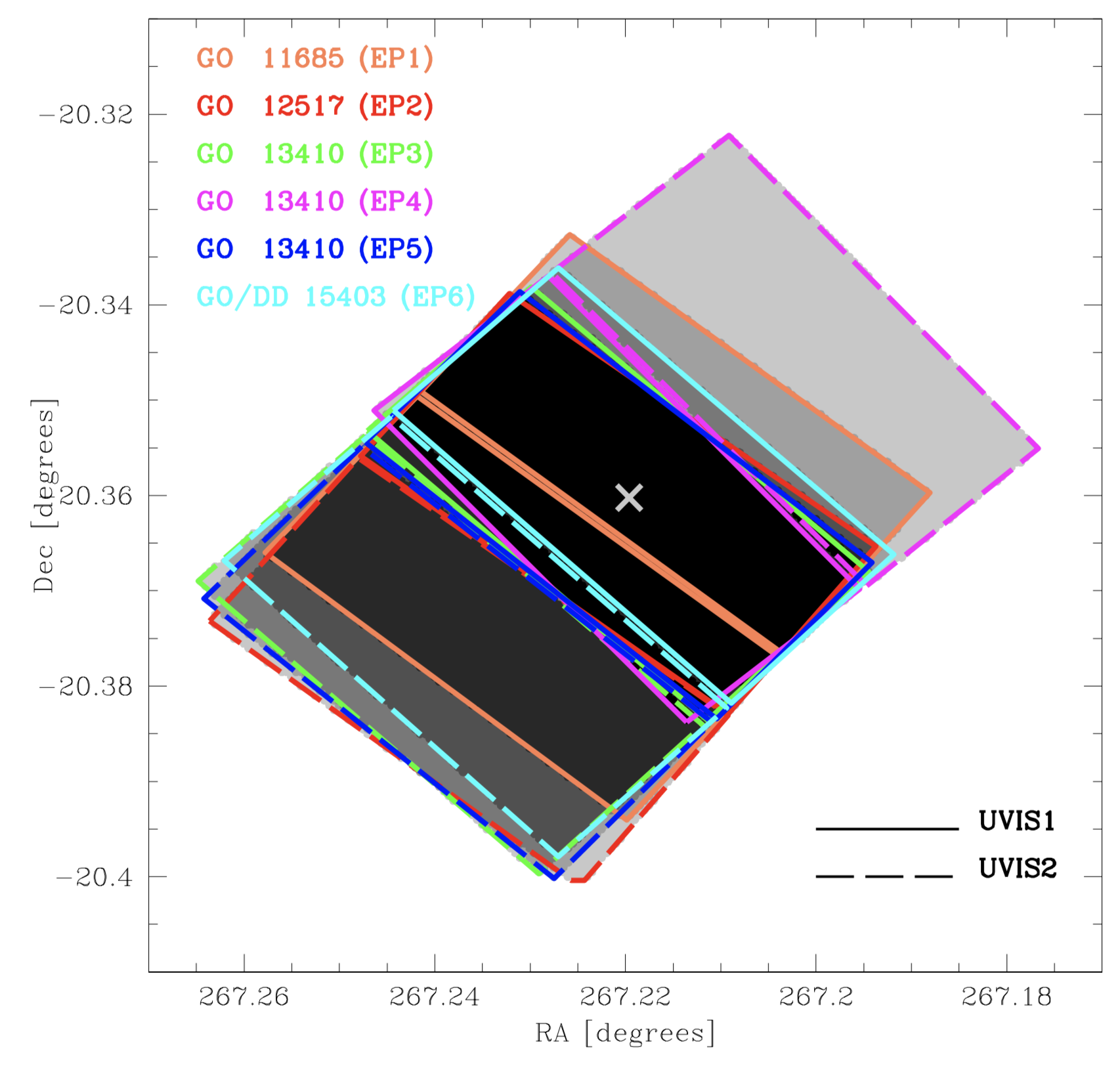
Figure 1: Total field of view sampled by the observations. The cross marks the cluster center (Harris, 1996, 2010 version). Solid and dashed lines identify the UVIS1 and UVIS2 chips of the WFC3, respectively, while different colors represent different epochs (see the legend in Figure). Different regions are shaded with increasingly dark grey colors as a function of increasing number of images overlapped in those portions of the FOV. These range from only one in the case of most of UVIS2 of GO 13410 (EP4) up to all the six epochs at the cluster center

2.2 Photometric analysis, astrometry and magnitude calibration

The data reduction procedure has been performed independently on each different epoch (see Table 1) and detector (UVIS1 and UVIS2) onto the CTE-corrected (flc) images after a correction for Pixel-Area-Map by using standard IRAF procedures. The photometric analysis has been carried out by using the DAOPHOT package (Stetson, 1987). For each image we first modelled the point spread function (PSF) by using a large number ($\sim 200$) of bright and nearly isolated stars. The adopted PSF consists of an analytical MOFFAT model plus a second order spatially variable look up table. We then performed a source search onto all single images imposing a $5\sigma$ threshold to the F606W and F814W images and $10\sigma$ to F656N images. We used such a conservative threshold in order to have a catalog free from spurious objects, while keeping a relatively high number of sources.

After applying the PSF previously modelled to each single image, we constructed a master list for each combination of epoch and detector, considering as reliable sources all the objects measured in more than half of the images in at least one filter. We then run the ALLFRAME package (Stetson, 1987, 1994) onto all the images of each single group “epoch/detector” by using the master list above. The final catalogs (one per each epoch and detector) contain all the objects measured in at least 2 filters. For each star, they list the instrumental coordinates, the mean magnitude in each filter and two quality parameters (chi and sharpness).

The instrumental magnitudes of each “epoch/detector” catalog have been independently calibrated to the VEGAMAG system by using the photometric zero points and the procedures reported on the WFC3 web page. In order to guarantee the photometric homogeneity of the catalogs, we used the large number of stars in common among different catalogs to quantify and correct any residual photometric offsets. To this aim, we adopted the EP2/UVIS1 catalog as reference since this pointing has the largest photometric accuracy, thanks to its largest number of exposures (see Table 1), and it samples the cluster center. Very small residuals (smaller than 0.05 mag) have been measured and applied to the photometric catalogs to match the reference.

It is well known that WFC3 images are affected by geometric distortions within the FOV, hence we corrected the instrumental positions of the stars in each catalog by applying the equations and the lookup table reported by Bellini et al. (2011).

Finally, since a non negligible contamination from field stars is expected, the distortion-corrected catalogs have been placed onto the International Celestial Reference System (ICRS) (GAIA DR2; Gaia Collaboration et al., 2016a, b; Lindegren et al., 2018) by using only a sub-sample of stars with large probability to be cluster members. To this end, we performed a first-order estimate of the stellar proper motions, as described in the next Section.

3 RELATIVE PROPER MOTIONS

NGC 6440 is a GC located in the Milky Way bulge, hence a strong contamination by field stars (both of disk and bulge) is expected. Given the procedure adopted in this work to estimate the differential reddening (see Section 4), a separation of the cluster population from the field is useful to better constrain the extinction. Unfortunately, the comparison between a Galaxy simulation in the direction of NGC 6440 (Robin et al., 2003, 2004) and the cluster absolute proper motion measure (Gaia Collaboration et al., 2018) showed that NGC 6440 is moving in the same direction of all the Milky Way populations (both disk and bulge) on the plane of the sky, making decontamination of the sample from field star interlopers quite complex in this case.

While the detailed analysis of proper motions will be presented in a forthcoming paper (Pallanca et al., 2019, in preparation), here we illustrate just the main steps of the procedure that we adopted to obtain a first-order separation of cluster members from field stars.

Table 1 shows that our sample contains a large number of repeated exposures with a relatively large acquisition time separation (up to 8 yrs). In principle, we could use only the pair of epoch separated by the largest temporal baseline (i.e., EP1 and EP6), in order to obtain a first-order separation of cluster and field stars. However, these two epochs are those with the smallest number of acquired exposures (only two per filters; see Table 1), hence they are not ideal to get high photometric accuracy and consequently accurate centroid positions (which are crucial to derive high-quality proper motion measures). Thus, we decided to consider all the epochs in order to maximise both the number of measurements in as many epochs as possible, and the size of the sampled FOV. Moreover, to minimise the effect of possible field contamination in the sample of stars used to compute the coordinate transformation, we adopted a two-step procedure. In the first step we indeed combined EP1 and EP6 only (i.e., the most distant in terms of time) to build a zero-order vector point diagram (VPD), which we used to make a pre-selection of bona fide member stars distributed along the entire FOV, by excluding the most evident field interlopers. We then matched the list of these candidate members with the VVV survey (Catelan et al., 2011; Chené et al., 2012) sample in the direction of NGC 6440, after placing the latter on the ICRS astrometric system through cross-correlation with Gaia DR2 data, used as astrometric reference. In the second step we reported all the single epoch positions to the reference system of the bona fide member star catalog and we calculated the final proper motion taking into account (for each star) all the centroid measurements from all the epochs. To this aim, for each star we fitted all the known positions with a $\chi^{2}$ method according to the following equations:

$$RA_{\rm obs}=\Delta RA\cdot(MJD_{\rm obs}-MJD_{\rm 2000})+RA_{\rm 2000}$$ (1)

$$Dec_{\rm obs}=\Delta Dec\cdot(MJD_{\rm obs}-MJD_{\rm 2000})+Dec_{\rm 2000}$$ (2)

where $RA_{\rm obs}$, $Dec_{\rm obs}$ and $MJD_{\rm obs}$ are the coordinates and the modified Julian day of each single observation, while $RA_{\rm 2000}$ and $Dec_{\rm 2000}$ are the positions at the reference epoch J2000. The final relative proper motions are $\mu_{\alpha}=14600\cdot\Delta RA$ and $\mu\delta=14600\cdot\Delta Dec$ expressed in mas/yr. The final VPD is reported in Figure 2.

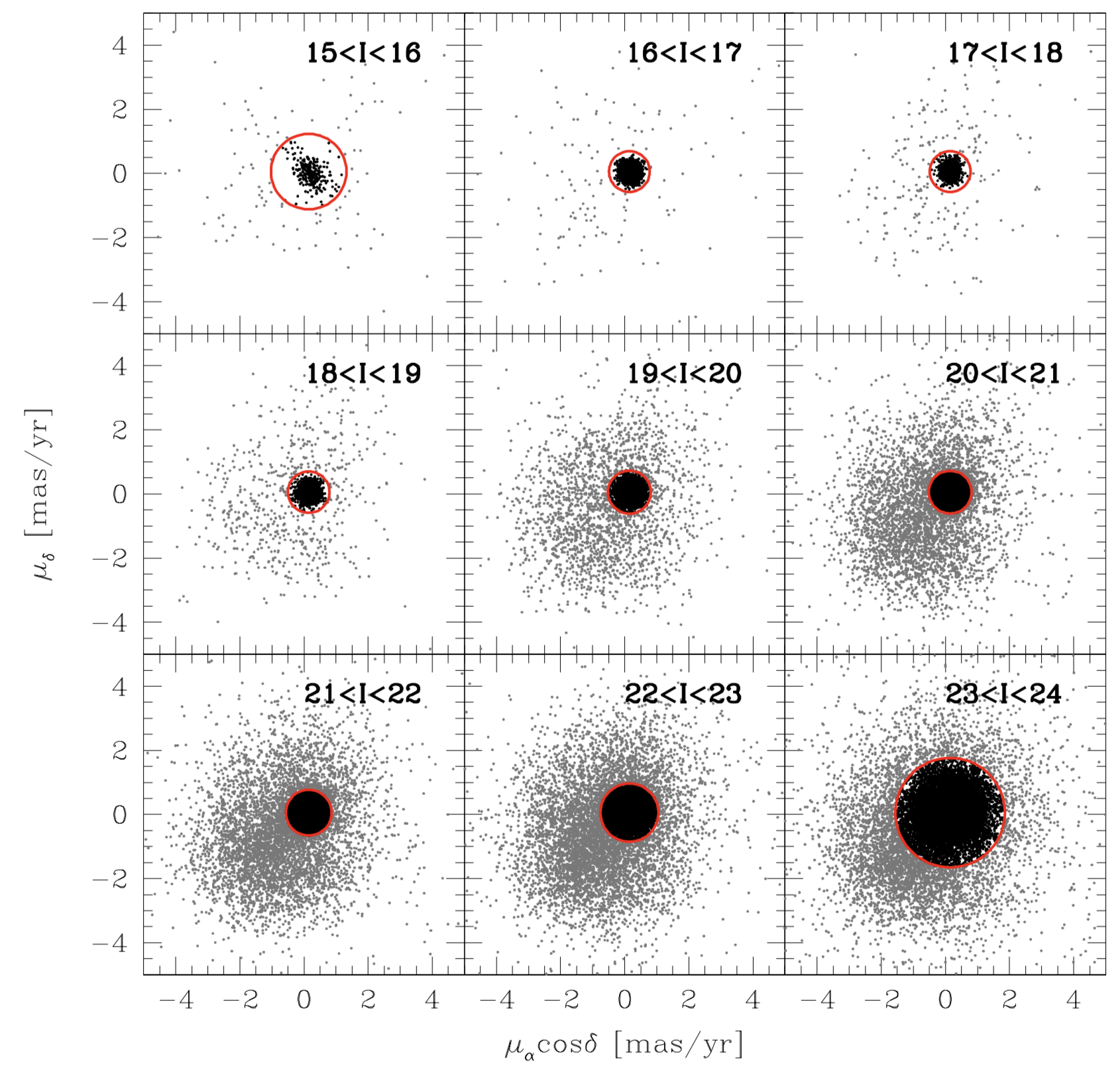
Figure 2: Vector point diagram for the magnitude bins labelled in each panel. The red circles mark the adopted radii (see text for details on its determination) to separate cluster stars (black dots) from field stars (gray dots). Clearly, the two populations are overlapped in the VPD, hence a complete decontamination is impossible.

As expected, the cluster stars appear as a bulk of points with a highly peaked proper motion distribution around the origin of the VPD, while field stars follow a much more dispersed distribution. Although the significant overlap between the two distributions in the VPD prevents a complete decontamination from the field interlopers, the significantly different shape of the two distributions surely allows to perform a first-order identification of likely field interlopers. To this end, we estimated the dispersion ($\sigma_{PM}$) of the proper motion distribution around the origin of the VPD in each magnitude bin and assumed the $2.5\sigma_{PM}$ radius as a “cluster confidence” radius ($r_{cc}$), able to separate the portion of the VPD dominated by cluster stars ($r<r_{cc}$) from that dominated by field interlopers ($r>r_{cc}$). In the following, according to what is shown in Figure 2, we consider cluster members those stars lying in the VPD at $r<r_{cc}$, being aware that a residual field contamination is present. The resulting CMDs, obtained from the selected cluster members and field interlopers separately, are shown in Figure 3 for each epoch.

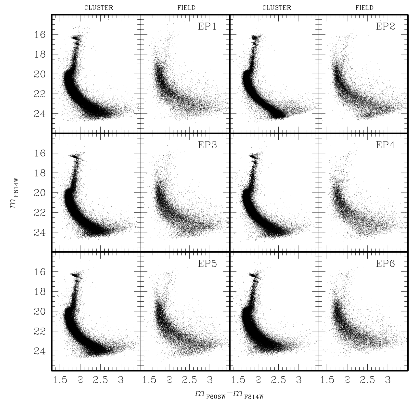
Figure 3: For each epoch (see labels) two CMDs are shown: in the left panel we plotted all the candidate member stars, while in the right panel we show the non member stars, according to the selection shown in Figure 2.

4 DIFFERENTIAL REDDENING

The aim of this work is to derive a differential extinction map in the direction of the globular cluster NGC 6440, at the highest spatial resolution achievable with the available data. To do this, we adopted a procedure already tested in previous works (see, e.g., Milone et al. 2012; Bellini et al. 2013; Saracino et al. 2019), also taking into account the dependence of the extinction coefficients on the effective temperature of the stars. As discussed in the Introduction, to maximise the spatial resolution here we adopted the “star by star” approach and used the sources observed along the RGB, SGB and bright MS. As a preliminary step, we assigned a temperature to each star, using a DSED isochrone model (Dotter et al., 2008). We then dereddened the observed magnitudes according to the relations of Casagrande, & VandenBerg (2014). On this preliminary dereddened diagram ($m_{\rm F606W,0}-m_{\rm F814W,0}$, $m_{\rm F814W,0}$), we computed the dereddened mean ridge line (D-MRL). To this end, we divided the considered portion of the CMD in different magnitude bins, and in each bin we computed the mean color after a $3\sigma$-clipping rejection. We adopted variable mag-wide bins (ranging from 0.2 to 0.5 mag) in order to best sample the morphology changes of the sequences in the MS Turn-Off region. In order to compute the D-MRL, we used only stars in the “reference” catalog (EP2/UVIS1), sampling the cluster core with the highest photometric quality (see Section 2.2). Moreover, only cluster member candidates (as selected from the relative proper motions as described in the previous section) have been considered. This sample was further cleaned by applying a 3-sigma rejection on the chi and sharpness parameters. The D-MRL was further refined onto the first-step differential reddening corrected catalog and then applied to all the photometric catalogs. The final D-MRL is shown (as a green line) in Figure 4 .

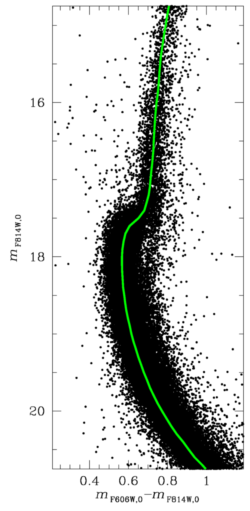
Figure 4: Dereddened cluster reference mean-ridge line (D-MRL, in green) obtained from the plotted sub-sample of stars (black dots) selected as described in Section 4.

The procedure then consists in determining, per each star in the catalog, the value of ${\rm E}(B-V)$ required to shift the D-MRL line along the direction of the reddening vector to fit the CMD drawn by $N_{*}$ sources spatially lying in the neighborhood of that star. The ideal number of stars ($N$) for sampling the CMD would be a few dozens. However, to keep the spatial resolution as high as possible, we introduced a complementary input parameter defined as the limiting radius ($r_{\rm lim}$) of a circle centred on each star, including the sources used to build the CMD. We set $N=30$ and $r_{\rm lim}=10\arcsec$. As soon as one of these two conditions is satisfied, the other is not considered anymore. Typically, the number of stars ($N_{*}$) within a $10\arcsec$ radius is much larger than $N=30$ in the inner cluster regions, while the opposite is true in the outskirts. Hence, the typical input parameter used at small radii is $N$, while it becomes $r_{\rm lim}$ at large cluster-centric distances.

So, following either the $N$ or the $r_{\rm lim}$ criterion, for each star of the catalog we selected from the bona fide star list the $N_{*}$ closest objects in the magnitude range $17.5<m_{\rm F814W}<21.5$. We then shifted the D-MRL along the reddening direction in steps of ${\rm E}(B-V)$ by adopting the absorption coefficients calculated as a function of the wavelengths and effective temperature of the targets (Casagrande, & VandenBerg, 2014). For each ${\rm E}(B-V)$ step, we calculated the residual color $\Delta VI$ defined as the difference between the $(m_{\rm F606W}-m_{\rm F814W})=VI$ color observed for each of the $N_{*}$ selected objects ($VI_{\rm obs}$) and that of the shifted D-MRL at the same level of magnitude ($VI_{\rm MRL}$), plus a second term where this color difference is weighted by taking into account both the photometric color error ($\sigma$) and the spatial distance ($d$) from the central star, according to the following equations:

$$\Delta VI=\sum_{i=1}^{N_{*}}\left(\left|{VI_{{\rm obs},i}-VI_{{\rm MRL},i}}\right|+w_{i}\cdot\left|{VI_{{\rm obs},i}-VI_{{\rm MRL},i}}\right|\right)$$ (3)

and

$$w_{i}=\frac{1}{d_{i}\cdot\sigma_{i}}\left[{\sum_{j=1}^{N_{*}}\left(\frac{1}{d_{j}\cdot\sigma_{j}}\right)}\right]^{-1}$$ (4)

The second term is meant to give more importance to the closest stars (for a good spatial resolution of the resulting map), avoiding biases due to the use of a too large $r_{\rm lim}$. Note that we cannot reduce the equation (3) to the second term only, because a bright object (with small photometric errors) close to the central star would dominate the weight and make the reddening estimate essentially equal to the value needed to move the D-MRL exactly on that object. We also performed a $3\sigma$ rejection in order to discard stars with a color distance from the D-MRL significantly larger than that of the bulk of the selected objects. This is useful to exclude field interlopers and/or discard non canonical stars (Pallanca et al., 2010, 2013, 2014; Cadelano et al., 2015a; Dalessandro et al., 2014; Ferraro et al., 2015, 2016a) with intrinsic colors different from those of the cluster main populations. The final differential reddening value assigned to each star is the value of the ${\rm E}(B-V)$ step that minimises the residual color ($\Delta VI$).

5 DISCUSSION AND CONCLUSIONS

We applied the procedure described in the previous section to each “epoch/detector” catalog by following two different approaches. In the assumed magnitude range ($17.5<m_{\rm F814W}<21.5$) we considered: (1) all the measured stars; (2) only the bona-fide cluster stars, selected for the chi and sharpness values that also survived to the proper motion selection. Note that the first approach maximises the total spatial extension of the reddening map, since it allows to explore also the North-West portion of the FOV, which has been observed only in one epoch (EP4) and for which proper motions cannot be computed.

In Figure 5 we show the differential reddening maps obtained for all the six epochs with the two approaches. These have been derived directly from the values of ${\rm E}(B-V)$ calculated per each single star, visualising as a colormap the spatial behaviour of the reddening with a nominal resolution of a few $0.1\arcsec$. Obviously, each epoch covers slightly different regions of the total FOV with significant overlaps. In the panels sampling the same region of the sky, it is possible to recognise the same main structures. In particular a main feature is visible in all the panels: a sort of high-extinction filament crossing the South-West portion of the cluster. Other reddening filaments are visible crossing the cluster center approximately in the North-South direction. Moreover, from the direct comparison of the reddening values obtained, we found an extreme level of homogeneity among different epochs and between the two approaches. This is somehow expected because of the adopted method, but it testifies the correct application of the procedure and guarantees that the method is poorly affected by the presence of field interlopers.

Figure 5: Reddening maps, centred onto the cluster center (Harris, 1996), for the 6 different epochs and for the two approaches adopted here: by using only bona fide cluster members and all stars (see labels). Thick black lines mark for clarity the contour of the total FOV. The top colorbar codifies the ${\rm E}(B-V)$ values ranging from less extinct regions (white colors) up to more absorbed areas (darker colors).

To quantify the agreement between the two approaches, we directly compared the two corresponding global extinction maps. To do that, we created a uniform grid of cells with side $0.5\arcsec$ and to each cell we assigned the average ${\rm E}(B-V)$ calculated as the median of all the available values (i.e. all the values assigned to all the stars within each cell in different epochs). Figure 6 shows the extinction maps obtained for both approaches and the “residual maps” resulting from their difference in the region in common. As can be seen the residual map is essentially flat, showing an average value lower than $~{}5\%$, thus demonstrating that both the intensity and the spatial displacement of the main features are consistently estimated in the two approaches.

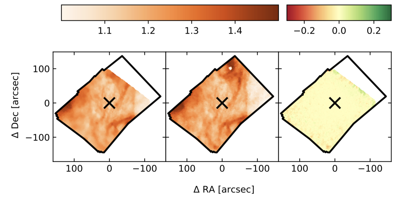
Figure 6: Global reddening maps computed adopting the two approaches described in the text: by using only bona fide cluster members (left panel) and all stars (central panel). The white spot located in the northern part of the FOV is due to the presence of a very bright (foreground) star that prevents the estimation of the local reddening. The residual map resulting from the difference of the two maps in the overlapping region is shown in the right panel. In each panel the center of the cluster is marked with a black cross, North is up and East is on the left. The thick black line marks for clarity the contour of the total FOV. The top-left colorbar codifies the ${\rm E}(B-V)$ values with respect to the D-MRL, ranging from less extinct regions (lighter colors) up to more absorbed areas (darker colors). The top-right colorbar shows the colors assigned to the residual values.

The differential reddening corrected CMDs, where the magnitudes and colors of each star have been corrected by using the values estimated through the “bona-fide” approach, are shown in Figure 7. Although the calculated reddening map is appropriate for cluster stars and not necessarily suitable for the field population, we show the effect of the correction on both the cluster and the field members. The comparison with Figure 3 highlights the clear improvement in the quality of the CMDs obtained thanks to the the differential reddening correction: indeed all the main evolutionary sequences in the CMD are thinner and better defined. To quantify the effectiveness of the correction, we estimated the width of the cluster faint RGB (in the range $16.5<m_{\rm F814W,0}<15.5$) before and after the correction: the dispersion in color decreases by more than a factor of 2, from $=0.05$ mag down to $=0.02$ mag.

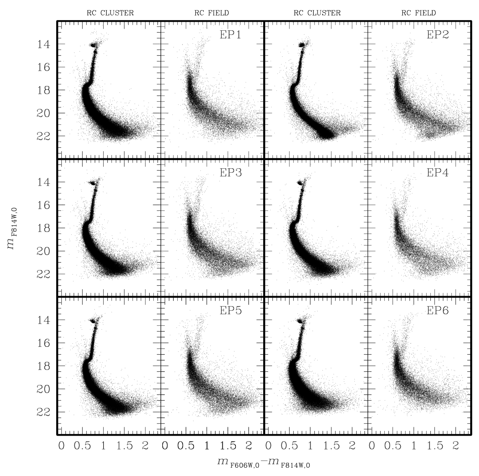
Figure 7: For each epoch (see labels) two reddening corrected (RC) CMDs are shown: in the left panel we plot all the candidate member stars, while the right panel shows the stars considered non members.

The central panel of Figure 6 shows the total differential reddening map in the direction of NGC 6440 computed in this study. It has a spatial resolution of only $0.5\arcsec$ and ${\rm E}(B-V)$ spans $\sim 0.5$ mag, ranging from $\sim 1$ to $\sim 1.5$ with a small tail at lower values. The most extincted region appears to be located in the northern portion of the cluster. Note that the white spot located in this region is an artifact due to a presence of a very bright foreground star that prevents the estimation of the local reddening. From this region a filamentary structure extends toward the cluster center. Indeed the quite large spatial resolution of the map nicely shows other filamentary structures crossing the FOV, as that visible in the South-West portion of the cluster. Another clumpy cloud is visible toward the East, while the West portion of the FOV shows a substantial drop of the extinction approximately starting from $\sim 70\arcsec$ West of the cluster center, showing an essentially vertical (North-South direction) edge.

Finally, Figure 8 reports the differential reddening corrected and chi and sharpness cleaned CMD for both candidate member stars (113765 objects; black points) and field stars (22873 stars; grey points). This is the cleanest and most accurate CMD obtained so far for NGC 6440. As can be seen, with the exception of the brightest portion of the RGB (saturated in these observations) all the evolutionary sequences are clearly defined. This dataset will be used in forthcoming studies aimed at deriving the physical structural parameters of the cluster (Pallanca et al, 2019, in preparation), by using the method presented in (Miocchi et al., 2013), and to explore the internal dynamics of the core by means of complementary radial velocity measures (Ferraro et al, 2019, in preparation) acquired in the contest of the MIKiS Survey (Ferraro et al., 2018b, c).

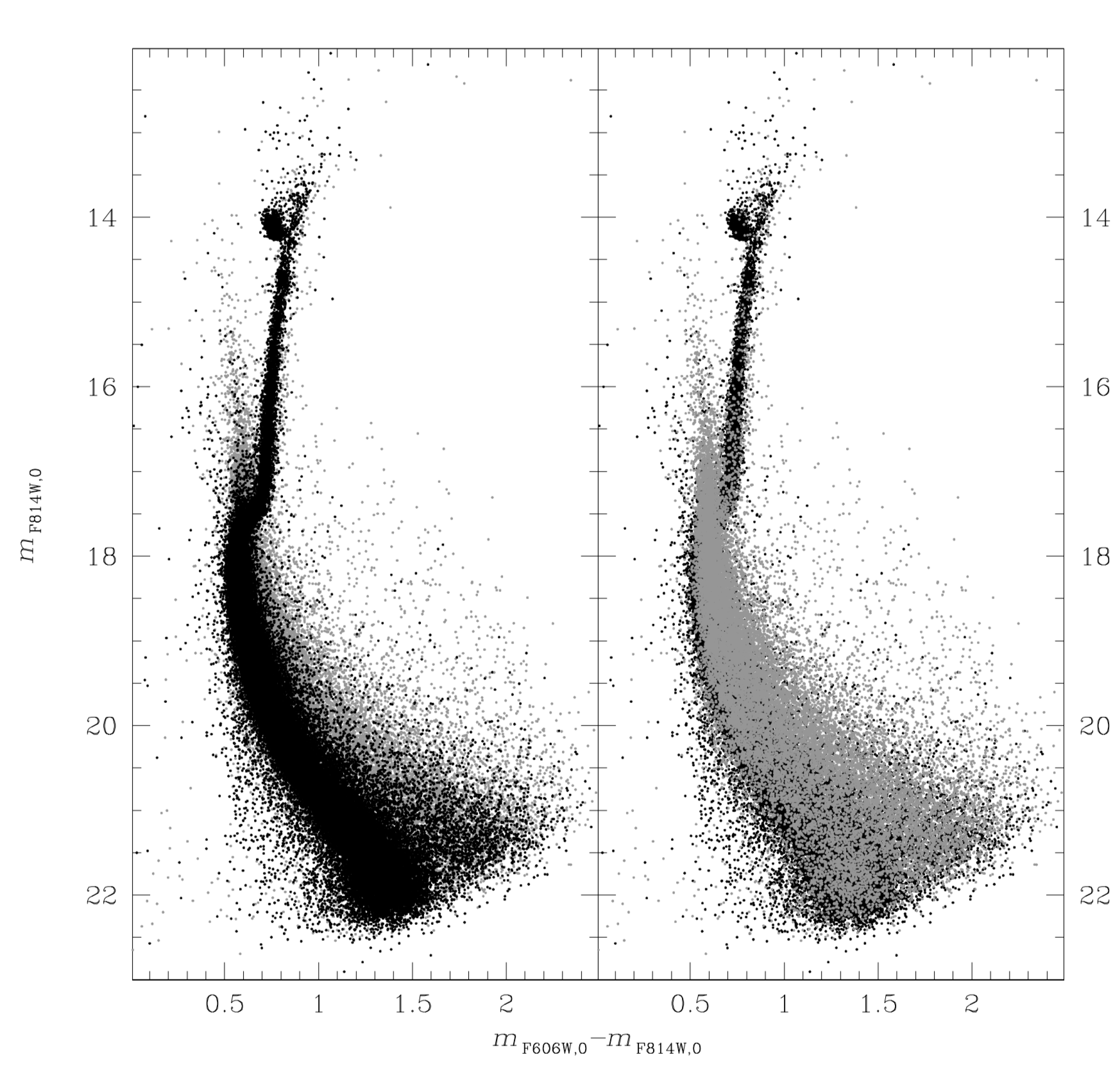
Figure 8: The cleanest CMD of NGC 6440 obtained so far. The figure shows only stars selected for the chi and sharpness parameters, with the magnitudes corrected for the effect of differential reddening. Black and grey dots correspond, respectively, to stars which are likely cluster members and field interlopers (as determined from the proper motion analysis). To more clearly illustrate the CMD location of field stars with respect to the cluster population, the grey dots are plotted behind and in front of the black dots in the left and right panels, respectively.

References

- Alonso-García et al. (2011) Alonso-García, J., Mateo, M., Sen, B., Banerjee, M., & von Braun, K. 2011, AJ, 141, 146
- Altamirano et al. (2010) Altamirano, D., Patruno, A., Heinke, C. O., et al. 2010, ApJ, 712, L58
- Bailyn (1995) Bailyn, C. D. 1995, ARA&A, 33, 133
- Beccari et al. (2019) Beccari et al 2019, arXiv:1903.11113
- Bellini et al. (2011) Bellini, A., Anderson, J., & Bedin, L. R. 2011, PASP, 123, 622
- Bellini et al. (2013) Bellini, A., Piotto, G., Milone, A. P., et al. 2013, ApJ, 765, 32
- Bonatto et al. (2013) Bonatto, C., Campos, F., & Kepler, S. O. 2013, MNRAS, 435, 263
- Cadelano et al. (2015a) Cadelano, M., Pallanca, C., Ferraro, F. R., et al. 2015a, ApJ, 807, 91
- Cadelano et al. (2015b) Cadelano, M., Pallanca, C., Ferraro, F. R., et al. 2015b, ApJ, 812, 63
- Cadelano et al. (2017a) Cadelano, M., Pallanca, C., Ferraro, F. R., et al. 2017a, ApJ, 844, 53
- Cadelano et al. (2019) Cadelano, M., Ferraro, F. R., Istrate, A. G., et al. 2019, ApJ, 875, 25
- Cardelli et al. (1989) Cardelli, J. A., Clayton, G. C., & Mathis, J. S. 1989, ApJ, 345, 245
- Casagrande, & VandenBerg (2014) Casagrande, L., & VandenBerg, D. A. 2014, MNRAS, 444, 392
- Catelan et al. (2011) Catelan, M., Minniti, D., Lucas, P. W., et al. 2011, RR Lyrae Stars, Metal-Poor Stars, and the Galaxy, 5, 145
- Chené et al. (2012) Chené, A.-N., Borissova, J., Clarke, J. R. A., et al. 2012, A&A, 545, A54
- Dalessandro et al. (2014) Dalessandro, E., Pallanca, C., Ferraro, F. R., et al. 2014, ApJ, 784, L29
- Dotter et al. (2008) Dotter, A., Chaboyer, B., Jevremović, D., et al. 2008, ApJS, 178, 89
- Ferraro et al. (2001) Ferraro, F. R., Possenti, A., D’Amico, N., & Sabbi, E. 2001, ApJ, 561, L93
- Ferraro et al. (2003) Ferraro, F. R., Possenti, A., Sabbi, E., & D’Amico, N. 2003, ApJ, 596, L211
- Ferraro et al. (2009a) Ferraro, F. R., Beccari, G., Dalessandro, E., et al. 2009a, Nature, 462, 1028
- Ferraro et al. (2009b) Ferraro, F. R., Dalessandro, E., Mucciarelli, A., et al. 2009, Nature, 462, 483
- Ferraro et al. (2012) Ferraro, F. R., Lanzoni, B., Dalessandro, E., et al. 2012, Nature, 492, 393
- Ferraro et al. (2015) Ferraro, F. R., Pallanca, C., Lanzoni, B., et al. 2015, ApJ, 807, L1
- Ferraro et al. (2016a) Ferraro, F. R., Lapenna, E., Mucciarelli, A., et al. 2016, ApJ, 816, 70
- Ferraro et al. (2016b) Ferraro, F. R., Massari, D., Dalessandro, E., et al. 2016, ApJ, 828, 75
- Ferraro et al. (2018a) Ferraro, F. R., Lanzoni, B, Raso, S., et al. 2018a, ApJ, 860, 36
- Ferraro et al. (2018b) Ferraro, F. R., Mucciarelli, A., Lanzoni, B., et al. 2018b, ApJ, 860, 50
- Ferraro et al. (2018c) Ferraro, F. R., Mucciarelli, A., Lanzoni, B., et al. 2018, The Messenger, 172, 18
- Freire et al. (2008) Freire, P. C. C., Ransom, S. M., Bégin, S., et al. 2008, ApJ, 675, 670-682
- Gaia Collaboration et al. (2016a) Gaia Collaboration, Brown, A. G. A., Vallenari, A., et al. 2016, A&A, 595, A2
- Gaia Collaboration et al. (2016b) Gaia Collaboration, Prusti, T., de Bruijne, J. H. J., et al. 2016, A&A, 595, A1
- Gaia Collaboration et al. (2018) Gaia Collaboration, Helmi, A., van Leeuwen, F., et al. 2018, A&A, 616, A12
- Gonzalez et al. (2011) Gonzalez, O. A., Rejkuba, M., Zoccali, M., Valenti, E., & Minniti, D. 2011, A&A, 534, A3
- Gonzalez et al. (2012) Gonzalez, O. A., Rejkuba, M., Zoccali, M., et al. 2012, A&A, 543, A13
- Harris (1996) Harris, W. E. 1996, VizieR Online Data Catalog, 7195,
- Heitsch & Richtler (1999) Heitsch, F., & Richtler, T. 1999, A&A, 347, 455
- Hunter (2007) Hunter, J. D., 2007, Computing in Science & Engineering, 9, 90
- Kerber et al. (2019) Kerber, L. O., Libralato, M., Souza, S. O., et al. 2019, MNRAS, 484, 5530
- Lanzoni et al. (2010) Lanzoni, B., Ferraro, F. R., Dalessandro, E., et al. 2010, ApJ, 717, 653
- Lanzoni et al. (2016) Lanzoni, B., Ferraro, F. R., Alessandrini, E., et al. 2016, ApJ, 833, L29
- Lanzoni et al. (2018a) Lanzoni, B., Ferraro, F. R., Mucciarelli, A., et al. 2018a, ApJ, 865, 11
- Lanzoni et al. (2018b) Lanzoni, B., Ferraro, F. R., Mucciarelli, A., et al. 2018b, ApJ, 861, 16
- Lindegren et al. (2018) Lindegren, L., Hernández, J., Bombrun, A., et al. 2018, A&A, 616, A2
- Massari et al. (2012) Massari, D., Mucciarelli, A., Dalessandro, E., et al. 2012, ApJ, 755, L32
- Massari et al. (2014) Massari, D., Mucciarelli, A., Ferraro, F. R., et al. 2014, ApJ, 795, 22
- Mauro et al. (2012) Mauro, F., Moni Bidin, C., Cohen, R., et al. 2012, ApJ, 761, L29
- McWilliam & Zoccali (2010) McWilliam, A., & Zoccali, M. 2010, ApJ, 724, 1491
- Milone et al. (2012) Milone, A. P., Piotto, G., Bedin, L. R., et al. 2012, A&A, 540, A16
- Miocchi et al. (2013) Miocchi, P., Lanzoni, B., Ferraro, F. R., et al. 2013, ApJ, 774, 151
- Minniti et al. (2010) Minniti, D., Lucas, P. W., Emerson, J. P., et al. 2010, New A, 15, 433
- Muñoz et al. (2017) Muñoz, C., Villanova, S., Geisler, D., et al. 2017, A&A, 605, A12
- Nataf et al. (2010) Nataf, D. M., Udalski, A., Gould, A., Fouqué, P., & Stanek, K. Z. 2010, ApJ, 721, L28
- Oliphant (2006) Oliphant T. E. 2006, Trelgol Publishing
- Origlia et al. (1997) Origlia, L., Ferraro, F. R., Fusi Pecci, F., & Oliva, E. 1997, A&A, 321, 859
- Origlia et al. (2008) Origlia, L., Valenti, E., & Rich, R. M. 2008a, MNRAS, 388, 1419
- Origlia et al. (2013) Origlia, L., Massari, D., Rich, R. M., et al. 2013, ApJ, 779, L5
- Origlia et al. (2019) Origlia, L., Mucciarelli, A., Fiorentino, G., et al. 2019, ApJ, 871, 114
- Ortolani et al. (1994) Ortolani, S., Barbuy, B., & Bica, E. 1994, A&AS, 108, 653
- Ortolani et al. (2017) Ortolani, S., Cassisi, S., & Salaris, M. 2017, Galaxies, 5, 28
- Pallanca et al. (2010) Pallanca, C., Dalessandro, E., Ferraro, F. R., et al. 2010, ApJ, 725, 1165
- Pallanca et al. (2013) Pallanca, C., Dalessandro, E., Ferraro, F. R., Lanzoni, B., & Beccari, G. 2013, ApJ, 773, 122
- Pallanca et al. (2014) Pallanca, C., Ransom, S. M., Ferraro, F. R., et al. 2014, ApJ, 795, 29
- Piotto et al. (1999) Piotto, G., Zoccali, M., King, I. R., et al. 1999, AJ, 118, 1727
- Piotto et al. (2002) Piotto, G., King, I. R., Djorgovski, S. G., et al. 2002, A&A, 391, 945
- Pooley et al. (2003) Pooley, D., Lewin, W. H. G., Anderson, S. F., et al. 2003, ApJ, 591, L131
- Ransom et al. (2005) Ransom, S. M., Hessels, J. W. T., Stairs, I. H., et al. 2005, Science, 307, 892
- Robin et al. (2003) Robin, A. C., Reylé, C., Derrière, S., & Picaud, S. 2003, A&A, 409, 523
- Robin et al. (2004) Robin, A. C., Reylé, C., Derrière, S., & Picaud, S. 2004, A&A, 416, 157
- Saracino et al. (2019) Saracino, S., Dalessandro, E., Ferraro, F. R., et al. 2019, ApJ, 874, 86
- Stetson (1987) Stetson, P. B. 1987, PASP, 99, 191
- Stetson (1994) Stetson, P. B. 1994, PASP, 106, 250
- Valenti et al. (2004) Valenti, E., Ferraro, F. R., & Origlia, L. 2004, MNRAS, 351, 1204
- Valenti et al. (2007) Valenti, E., Ferraro, F. R., & Origlia, L. 2007, AJ, 133, 1287
- von Braun & Mateo (2001) von Braun, K., & Mateo, M. 2001, AJ, 121, 1522