Collision Detection for Agents in Multi-Agent Pathfinding

Abstract

Recent work on the multi-agent pathfinding problem (MAPF) has begun to study agents with motion that is more complex, for example, with non-unit action durations and kinematic constraints. An important aspect of MAPF is collision detection. Many collision detection approaches exist, but often suffer from issues such as high computational cost or causing false negative or false positive detections. In practice, these issues can result in problems that range from inefficiency and annoyance to catastrophic. The main contribution of this technical report is to provide a high-level overview of major categories of collision detection, along with methods of collision detection and anticipatory collision avoidance for agents that are both computationally efficient and highly accurate.

1 Introduction

Multi-agent pathfinding (MAPF) is the problem of finding paths for a set of agents from respective start locations to goal locations in a shared space while avoiding conflicts. MAPF has applications in robotics, navigation, games, etc. The problem of detecting collisions between agents (robots, objects, players, etc.) is of central importance for MAPF. There is a fundamental trade-off between accuracy and computation time; more accurate collision detection is often preferred in systems with strict safety requirements (e.g. human transport) while others may trade accuracy for speed when safety is not an issue (e.g. games).

This technical report first provides definitions and background for collision detection, a broad overview and categorization of existing methods and summarizes the advantages and disadvantages of each. Then efficient and exact equations for collision detection for circular and spherical agents with constant velocity and initial velocity with constant acceleration are formally defined. Finally, conic equations for anticipatory collision avoidance for circular and spherical agents are introduced. Many examples are used to illustrate the problem for 2-dimensional spaces, however, the case of 3-dimensional spaces is directly applicable.

2 Background

Conflict detection is important for many problems with multiple moving agents. For the purposes of this technical report, agents have spatial locations and a physical shapes such as circles, spheres, polygons or polygonal meshes. Agents may only occupy one location at a time, situated using a reference point (?). In the case of navigation and routing problems for multiple agents, feasible joint solutions cannot be found or verified without proper conflict detection. A conflict represents a simultaneous attempt to access a joint resource. Depending on the target domain a conflict may have different meanings, for example when states have dimensions other than spatial components such as scheduling problems or resource allocation problems (e.g. allocating time slots for classrooms or coordinating memory and cpu allocation for processing jobs) or when abstract states are used such as in dimensionally-reduced spaces. Typically, when considering only temporospatial aspects, conflict detection is referred to as collision detection.

Collision detection has been extensively studied in the fields of computational geometry, robotics, and computer graphics. When selecting a method for checking conflicts we need to be cognizant of type I and type II errors (?), that is, false positives (reporting a conflict that does not actually occur) and false negatives (not reporting a conflict that actually does occur). A method that exhibits type II errors should never be used because type II errors can lead to infeasible solutions. A method that exhibits type I errors may be used, but may be incomplete or lead to sub-optimal solutions. In this section we provide a brief taxonomy of collision detection techniques for multiple moving agents.

This tech report focuses on solutions for segmented motion. Segmented motion is defined as a series of movements (or actions) for agents that have a discrete length. Segmented motion is the natural product of path planning for agents in discretized spaces such as grids, graphs and robotic latices. A segment of motion is defined by a pair of states: $\langle s_{start},s_{end}\rangle$ where $s_{start}$ is the state of the agent at the beginning of motion and $s_{end}$ is the state of the agent at the end of motion. For example, a state may be defined as a position and time $s=\langle x,y,t\rangle$ or it may also include velocity (and acceleration) components: $s=\langle x,y,\dot{x},\dot{y},t\rangle$; $s=\langle x,y,\dot{x},\dot{y},\ddot{x},\ddot{y},t\rangle$. The definition of states, including the number of dimensions will depend upon the application. A motion segment is continuous between $s_{start}$ and $s_{end}$, thus the transition between them must be kinematically feasible. Finally, a path is composed of a sequence of states $\pi=[s_{0},...,s_{d}]$, or alternately, a sequence of motions $\pi=[m_{0},...,m_{d}]$ where each $s_{end}\in m_{i}=s_{start}\in m_{i+1}$.

2.1 Geometric Containers

Figure 1: Collision detection using geometric containers. A collision is correctly detected between agents (a) and (b), but erroneously detected between (a) and (c).

Geometric containers encapsulate portions of segmented motion in time and space using polygons, polytopes or spheres (?). Then intersection detection is detected between the geometric containers of differing agents to determine if a collision has occurred. There are various approaches to intersection detection for stationary objects (?; ?).

In Figure 1 an example of this approach is shown which uses axis-aligned bounding boxes as geometric containers. The temporal dimensions are not shown, but each bounding box also has a temporal component. Agent (a), (b) and (c) take actions (represented as directed edges) to arrive at their goal. Axis-aligned bounding boxes are reserved for each of these edges, then an intersection check is carried out. Although a collision is correctly detected between (a) and (b), an erroneous collision is detected between (b) and (c). Although this approach is computationally fast, it will reserve more temporospatial area than necessary, especially when long edges are present in a path, resulting in the possibility of type I errors.

2.2 Incremental/Sampling-Based

Figure 2: Sampling-based collision detection. A collision is not detected between agents (a) and (b).

This approach involves translating objects along their trajectories incrementally and using static collision detection methods to detect overlaps at each increment. Figure 2 shows an example of this approach. Agents are translated to regular intervals along their trajectories, then intersection checks are performed at each interval. In contrast to the example in Figure 1, there is no erroneous collision detected (type I error) between agent (a) and agent (c). However, a false negative (type II error) occurs between agent (a) and (b). The sampling approach is very important, samples too far apart may leave a collision undetected, but samples very close together are computationally costly. Adaptive sampling approaches can help improve the accuracy and computational cost (?).

In grid worlds, Brezenham’s line algorithm (?), a coarse form of collision detection can be used for selecting a specific set of grid-squares covered by a trajectory and then checking whether multiple agents are in the same grid square at intersecting times. A tighter approach based on Wu’s antialiased line algorithm (?) is used in the AA-SIPP(m) (?) algorithm. These methods may cause type I errors, but are guaranteed to avoid type II errors.

2.3 Algebraic

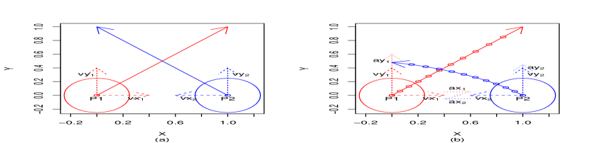
Figure 3: Algebraic collision detection for trajectories with (a) constant velocity and (b) initial velocity with constant acceleration

By parameterizing the trajectory, closed-form solutions to continuous-time conflict detection for circular, spherical, (?; ?) and triangular (?) shaped agents have been formulated. An example for circular agents is shown in Figure 3. In diagram (a), Agents move along their respective trajectories shown as a solid arrow. These trajectories are parameterized by the $x,y$ velocity vectors as shown with dashed arrows. Diagram (b) shows a similar scenario with acceleration vectors added to the tips of the velocity arrows shown with dotted arrows. Algebraic methods will calculate the exact time of collision between two moving agents assuming constant velocity and direction and also with acceleration.

When dealing with discrete-length motion segments, algebraic methods can be used to determine whether a collision will occur during the segment of motion. Deeper details of these calculations for circular agents are discussed in section 3.

2.4 Geometric

Figure 4: Constructive solid geometry collision detection. Time is extruded into the model as an extra dimension, after which polygonal intersection detection is performed.

Figure 5: Velocity Obstacle (VO) construction based on (a) two agents with motion vectors. The trajectories and shapes of agents are interpreted to create (b) the velocity obstacle – labeled ’VO‘

Geometric solutions are the most computationally expensive collision detection approaches, however they are formulated for many different obstacle shapes - typically primitive shapes, polygons or meshes. Two of the most popular approaches are constructive solid geometry (CSG) (?), and velocity obstacles (VO) (?).

CSG approaches treat the time domain as an additional polygonal dimension, extruding polygons into the time dimension, after which a static polygonal intersection check is applied. Computation of the extruded volumes can be very expensive and formulating ways to enhance CSG has been a subject of ongoing research (?; ?).

Velocity obstacles have been formulated for infinite length vector collision detection for arbitrary-shaped agents (?). A velocity obstacle is depicted in Figure 5. A VO is created for two agents $A$ and $B$, located with center points $A$ and $B$ as shown in diagram (a). The agents have shapes – here shown as circles with radius $r_{A}$ and $r_{B}$. The agents’ motion follows velocity vectors $VA$ and $VB$ shown as arrows.

In order to construct the VO, first, the shape of agent $B$ is inflated by computing the Minkowski sum $A\oplus B$ of the two agent’s shapes. Next, two tangent lines from point $A$ to the sides of $A\oplus B$ are calculated to form a polygon. Finally, the polygon is translated so that its apex is at $A+VB$. The area between the translated tangent lines is the velocity obstacle (labeled VO in the diagram). The VO represents the unsafe region of velocity for agent $A$, assuming agent $B$ does not change it’s trajectory. If the point $A+VA$ lies inside the VO, agent $A$ will collide with agent $B$ some time in the infinite future.

In the case of segmented motion, VOs can still be used for collision detection with some adaptations (?). In addition, collision avoidance can be achieved by choosing a velocity for $A$ such that $A+VA$ lies outside the VO. One approach is to set $VA$ so that $A+VA$ lies on the intersection point of either of the VO tangent lines $\pm\epsilon$.

2.5 Summary

Depending on the application, any of the above methods may meet the problem constraints. Static detection is the approach of choice for domains with discretized-time movement models as it is the cheapest and (depending on the movement model) may yield no loss in accuracy. In continuous-time domains, one of the latter choices is usually preferable, with sampling often being the cheapest approach, followed by algebraic and geometric approaches. There is a trade-off with respect to accuracy and computational cost. The latter approaches provide the most flexibility when high accuracy and complex agent shapes are necessary.

3 Closed-Form Collision Detection for Circular Agents

Figure 3 shows an example of two-agent motion for fixed velocity (a) and initial velocity with fixed acceleration (b). Computing the time and duration of conflict for two circular agents can be done by solving equations for the squared distance between agents (Ericson (2004)).

3.1 Constant Velocity

Given $P_{1}=\langle x_{1},y_{1}\rangle$, the start position of agent $1$, and $P_{2}=\langle x_{2},y_{2}\rangle$, the start position of agent $2$, velocity vectors $V_{1}=\langle vx_{1},vy_{1}\rangle$, $V_{2}=\langle vx_{2},vy_{2}\rangle$, and radii $r_{1}$, $r_{2}$ respectively, the location in time of an agent is defined as:

$$P^{\prime}=P+Vt$$ (1)

The following equation specifies the squared distance between the centers of the agents over time:

$$sqdist(t)={V_{\Delta}}^{2}t^{2}+2V_{\Delta}\boldsymbol{\cdot}P_{\Delta}t+{P_{\Delta}}^{2}$$ (2)

where

$P_{\Delta}=P_{1}-P_{2}$

$V_{\Delta}=V_{1}-V_{2}$

Via substitution, this equation is simplified to a quadratic equation:

$$sqdist(t)=at^{2}+bt+c_{0}$$ (3)

where

$a={V_{\Delta}}^{2}$

$b=2V_{\Delta}\boldsymbol{\cdot}P_{\Delta}$

$c_{0}={P_{\Delta}}^{2}$

A collision will occur when the squared distance between the agents is less than or equal to the squared sum of the radii, giving the following inequality.

$$at^{2}+bt+c_{0}\leq(r_{1}+r_{2})^{2}$$

Solving the inequality gives the equation for collision between the agent’s edges:

$$0\geq at^{2}+bt+c_{0}-(r_{1}+r_{2})^{2}$$

$$sqEdgeDist(t)=at^{2}+bt+c$$ (4)

where

$c=P_{\Delta}^{2}-(r_{1}+r_{2})^{2}$

Solving equation 4 for $t$ will determine the exact times where the squared distance between agent’s edges is zero – the time when collision occurs. Section 4 discusses the process for determining the conflict interval for using this equation.

3.2 Initial Velocity with Constant Acceleration

Equation $\eqref{eq:ctime3}$ can be extended for constant acceleration. Given $P_{1}=\langle x_{1},y_{1}\rangle$, the start position of agent $1$, and $P_{2}=\langle x_{2},y_{2}\rangle$, the start position of agent $2$, velocity vectors $V_{1}=\langle vx_{1},vy_{1}\rangle$, $V_{2}=\langle vx_{2},vy_{2}\rangle$, acceleration vectors $A_{1}=\langle ax_{1},ay_{1}\rangle$, $A_{2}=\langle ax_{2},ay_{2}\rangle$ and radii $r_{1}$, $r_{2}$ respectively, the location in time of an agent is defined as:

$$P^{\prime}=P+Vt+\frac{At^{2}}{2}$$ (5)

The following inequality specifies the collision condition as a quartic equation:

$$at^{4}+bt^{3}+ct^{2}+dt+e_{0}\leq(r_{1}+r_{2})^{2}$$ (6)

where

$a=\frac{{A_{\Delta}}^{2}}{4}$

$b={A_{\Delta}\boldsymbol{\cdot}V_{\Delta}}$

$c={A_{\Delta}\boldsymbol{\cdot}P_{\Delta}+V_{\Delta}}^{2}$

$d=2V_{\Delta}\boldsymbol{\cdot}P_{\Delta}$

$e_{0}={P_{\Delta}}^{2}$

for

$P_{\Delta}=P_{1}-P_{2}$

$V_{\Delta}=V_{1}-V_{2}$

$A_{\Delta}=A_{1}-A_{2}$

which gives the equation for the squared distance between circular edges:

$$sqEdgeDist(t)=at^{4}+bt^{3}+ct^{2}+dt+e$$ (7)

where

$e={P_{\Delta}}^{2}-(r_{1}+r_{2})^{2}$

Again, solving for $t$ will yield the time of collision, which is discussed further in the next section.

4 Computing the Exact Conflict Interval

The exact conflict interval is determined by solving for the roots of $\eqref{eq:ctime3}$ or $\eqref{eq:accel2}$ using the quadratic and quartic formulas respectively. These solutions assume that both agents are at $P_{1}$ and $P_{2}$ at the same time. However, if there is an offset in time, e.g. agent 1 starts moving at time $t_{1}$ and agent 2 starts moving at time $t_{2}$, then $P_{\Delta}$ must be adjusted to reflect this offset by projecting the position of the earlier agent to be at the position when the later agent starts its motion. If the earlier agent were agent 1, the adjustment would be as follows:

$$P_{\Delta}=P_{1}+V_{1}(t_{2}-t_{1})-P_{2}$$ (8)

Otherwise, the adjustment will be analogously done for agent 2. In the case of acceleration, the position and velocity must be adjusted (again, assuming agent 1 starts early) as:

$$P_{\Delta}=P_{1}+V_{1}(t_{2}-t_{1})+\frac{A_{1}(t_{2}-t_{1})^{2}}{2}-P_{2}$$ (9)

$$V_{\Delta}=V_{1}+A_{1}(t_{2}-t_{1})-V_{2}$$ (10)

4.1 Constant Velocity

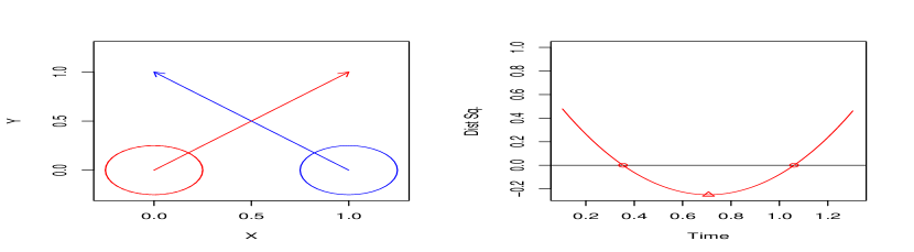
Figure 6: Agents Trajectories and Corresponding Squared Distance Plot

For the quadratic form, if the discriminant ($b^{2}-4ac$) is less than zero, $V_{1}$ and $V_{2}$ are parallel and no collision will ever occur. Assuming the discriminant is positive, the collision interval is defined as the roots of the quadratic formula:

$$t_{interval}=\frac{-b\pm\sqrt{b^{2}-4ac}}{2a}$$ (11)

In the case of a double root, the edges of the agents just touch, but no overlap actually occurs (assuming open intervals). See Figure 6 for an example of two-agent motion and the resulting squared-distance plot. When the distance is less than zero, there is overlap of the agents. Given this interval, it is possible to determine whether a collision will occur in the future and at what time, or if the agents are currently colliding.

4.2 Initial Velocity with Constant Acceleration

This case uses the quartic formula to find roots to $\eqref{eq:accel2}$. The quartic formula will yield 4 roots, some of which may be imaginary resulting in 0, 1 or 2 conflict intervals. Imaginary roots will tell us the time(s) at which agents are locally closest together, but do not actually overlap (local minima). Imaginary roots are always double roots, and can be discarded. If all 4 roots are imaginary, the agents never overlap. If there is a double real root, then the two agents touch edges at exactly one point in time, creating an instantaneous interval.

Because our equation is based on distance, the quartic function will always be concave up. Hence, the overlapping intervals can only be between roots 1,2 and 3,4. If roots 1,2 and/or 3,4 are real, then the agents continuously overlap between 1,2 and/or 3,4 respectively. Four real roots means that the objects overlap twice, continuously between root pairs 1,2 and 3,4. This is possible because agents may have curved trajectories. See Figure 3 (b) for an example.

5 Determining Exact Minimum Delay or Velocity Adjustment for Conflict Avoidance

It is often useful, not just to determine if and when agents are going to collide, but to determine a delay time to avoid collision.

5.1 Exact Delay for Constant Velocity

In order to determine the minimum delay required for an agent to avoid conflict, we adjust (3) to incorporate $\delta=t_{2}-t_{1}$, a delay variable, by plugging equation $\eqref{eq:adjust}$ into equation $\eqref{eq:ctime1}$ to get:

$$sqEdgeDist(t,\delta)=At^{2}+Bt\delta+C\delta^{2}+Dt+E\delta+F$$ (12)

where

$A={V_{\Delta}}^{2}$

$B=2(V_{1}^{2}-V_{1}\boldsymbol{\cdot}V_{2})$

$C={V_{1}}^{2}$

$D=2(P_{2}\boldsymbol{\cdot}V_{2}-P_{2}\boldsymbol{\cdot}V_{1}+P_{1}\boldsymbol{\cdot}V_{2}-P_{1}\boldsymbol{\cdot}V_{1})$

$E=-2(P_{2}\boldsymbol{\cdot}V_{1}+P_{1}\boldsymbol{\cdot}V_{1})$

$F={V_{\Delta}}^{2}-(r_{1}+r_{2})^{2}$

Equation $\eqref{eq:ellipse}$ is the standard form of a conic section. Note that the sign of both $A$ and $C$ are positive, therefore, this conic section will always be an ellipse, except for two degenerate cases: (1) agents’ motion is parallel and (2) at least one agent is waiting in place. Fortunately, both cases are easy to detect and solve. The conversion of (8) to canonical form for an ellipse will not be covered here, nor is it necessary.

Figure 7(a) shows an example of agent trajectories, the squared distance plot (equation (4)) when $delay=0$, and the resulting conic section (equation (12)). Note that the horizontal line at $\delta=0$ passes through the ellipse at the exact same time points that the squared distance plot does. If agent 1 were to delay by $\epsilon$, the horizontal line would move up, resulting in a different collision interval (see Figure 7(b)). If agent 2 were to delay by $\epsilon$, the horizontal line would move down, again resulting in a different collision interval. The question we want to solve is: what value of $delay$ will result in no collision? In other words, we want to find the positive value of $\delta$, such that the radii of the agents just touch, i.e. (12) yields a double root. The targeted delay interval is derived by determining the top and bottom extrema of the ellipse (?).

where $center_{\delta}$ is the y-coordinate of the ellipse center:

$center_{\delta}=\frac{BD-2AE}{4AC-B^{2}}$

The collision times of the endpoints of the delayRange are computed via:

$$collisionTimes=\frac{-B(delayRange)-D}{2A}$$ (14)

Note that (13) is undefined when the discriminant is negative, which can only happen for $a=0$ or $c=0$. This can only happen when agents’ motion vectors are parallel (moving the same or opposite directions) or either agent is waiting in place. These cases are easy to detect.

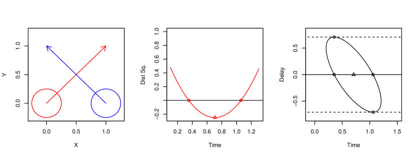
(a)

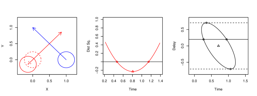
(b)

Figure 7: (a) Agent trajectories, squared distance plot and ellipse showing collision intervals for Varying $delay$ and (b) the same trajectories where the red agent is delayed delayed by 0.2 seconds

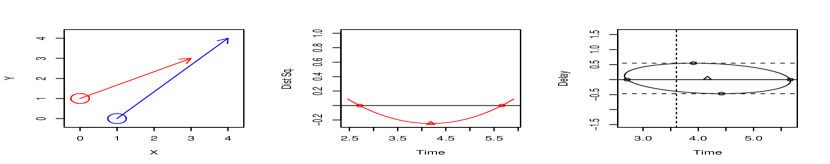
Figure 8: An example where the maximum delay time happens after the first agent arrives at its destination.

When the motion is not of infinite length, i. e. segmented motion, we must also take into account the beginning and end of the duration of motion. Effectively, we treat agents as if they appear at their start time and disappear at their end time. When the movement of agents 1 and 2 start at $t_{1}$ and $t_{2}$ and end at $t_{1}^{\prime}$ and $t_{2}^{\prime}$ respectively, we measure time relative to $t_{0}=MIN(t_{1},t_{2})$ and $t_{max}=MIN(t_{1}^{\prime},t_{2}^{\prime})$. In the case that $\delta=t_{1}-t_{2}$ is outside of the range $delayRange$ as calculated via (13), no collision will occur. If either of the collision times (as calculated in (14) for each point in $delayRange$ occur before $t_{0}$, or after $t_{max}$, the delay times need to be re-computed for $t_{0}$ or $t_{max}$ as necessary using (15). An example where $t_{max}$ occurs too early is shown by the vertical dashed line in Figure 8.

This yields the algorithm detailed in Algorithm 1 for computing the unsafe interval for segmented motion. The algorithm is straightforward and utilizes the following additional formulas:

The value of $\delta$, given a time which is derived from (12), solved for $\delta$:

$$\delta=\frac{-\sqrt{(Bt+E)^{2}-4C(t(At+D)+F)}+Bt+E}{2C}$$ (15)

The leftmost $t$ coordinate on the ellipse:

where $center_{t}$ is $\frac{BE-2CD}{4AC-B^{2}}$

At Algorithm 1, lines 5-9 check the actual delay ($\delta=t2-t1$) between the two agents against the unsafe delay range per equation (13). If there is no collision (e.g. in the case of parallel movement) or $\delta$ does not fall inside the unsafe range, no collision will occur. Lines 10-23 compute the unsafe time interval per equation (14) and then adjust the endpoints accordingly per t0 and tmax using equation (15).

The final result is the adjusted unsafe interval for agent 1. This interval can now be used to instruct agent 1 not to start execution of its action inside the interval (e.g. by starting its action sooner or later). Note that the unsafe interval for agent 2 is the negated interval for agent 1 – [-range[2],-range[1]].

Algorithm 1 Unsafe Interval Computation for Segmented Motion

1:INPUT: P1,P2,V1,V2,t1,t2,t1’,t2’,r1,r2

2:t0=MAX(t1,t2)

3:tmax$\leftarrow$MIN(t1’,t2’)

4:$\delta$=t2-t1

5:// Execute equation (13) to get unsafe delay range

6:range$\leftarrow$delayRange(P1,P2,V1,V2,r1,r2)

7:if range=$\emptyset$ or range[1]$>\delta$ or range[2]$<\delta$ then

8:     return NO COLLISION

9:end if

10:// Execute equation (14) to get unsafe time range

11:collisionTimes$\leftarrow$delayTimes(P1,P2,V1,V2,r1,r2)

12:minCollisionTime$\leftarrow$MIN(collisionTimes)

13:maxCollisionTime$\leftarrow$MAX(collisionTimes)

14:// Truncate delay for motion time segments

15:if minCollisionTime$<$t0 then

16:     // Get delay for t0 via (15)

17:     range[1]$\leftarrow$delayAtTime(P1,P2,V1,V2,r1,r2,t0)

18:end if

19:if maxCollisionTime$<$t0 then

20:     // Get delay for tmax via (15)

21:     range[2]$\leftarrow$delayAtTime(P1,P2,V1,V2,r1,r2,t0)

22:end if

23:// Return the unsafe interval by adding the delay to the start time

24:return [t0+range[1],MIN(tmax,t0+range[2])]

5.2 Exact Delay for Initial Velocity with Constant Acceleration

The equivalent conic equation for 4th order bivariates is called a quartic plane curve. A closed-form solution for unsafe intervals is still an open question. However, an interative solution has been formulated for the constant velocity case which is generalizable to this case (?).

The algorithm starts by evaluating (7) at $t0$, retrieving an initial upper bound from the interval which is closest to and greater than $t0$. Then performs a binary search, from both ends of the interval until the interval is determined within a predetermined accuracy threshold. Binary search is a well known algorithm and will not be repeated here.

5.3 Minimum Velocity Change for Constant Velocity

Figure 9: Velocity Obstacle (VO) construction based on (a) two agents moving on edges. (b) The minimum change for safe velocity is determined by the intersection points of the edge and the velocity obstacle.

In order to determine the minimum velocity change necessary to avoid collision for segmented motion, a VO is created as shown in Figure 9 which is similar to Figure 5, but with motion segments added. Motion segments are shown as dotted arrows with large points at the beginning and end of the segment. Velocities that lie on the segment are the only valid choices, hence a velocity that lies just outside of the VO as shown in diagram (b) is desirable for determining the minimum necessary change to avoid collision. There may be kinematic constraints on agents, such as a maximum velocity.

The following steps can be undertaken to determine the appropriate action for the agent, which may result in the agent waiting in place or using a new velocity:

1. Detect if a collision will occur inside the segments. This can be done via equation (4).

   • Return if no collision

2. Construct a VO, then compute a new velocity that lies on the segment and intersects with the edges of the VO as shown in Figure 9 (b) for agent A. Ths can be done using a formula for the line intersection point (?) of the motion vector and both of the VO tangent lines.

   • Return new velocity if either of the velocities at the intersection points are kinematically feasible.

3. Construct and check a VO for a new velocity for agent B.

   • Return new velocity if either of the velocities at the intersection points are kinematically feasible.

4. If the current state of the agent will allow it to wait in place, compute the delay using Algorithm 1.

   • Return original velocity and new delay.

5. Otherwise, return NO SOLUTION

6 Conclusion

In this paper, we have provided an overview of collision detection for polygonal and circular agents. We have also provided derivations for computing the exact interval of collision between two agents with constant velocity or intial velocity with constant acceleration. We have additionally derived a formulation for computing unsafe intervals (the range of start times in which agents come into collision) for two circular agents with constant velocity and differing start times. An algorithm was then shown for computing the unsafe intervals in the case of segmented motion. Finally, an algorithm for computing safe velocities and delay times was outlined.

Future work may involve derivations of the exact formulation of unsafe intervals for agents with acceleration.

References

- [Andreychuk et al. 2019] Andreychuk, A.; Yakovlev, K.; Atzmon, D.; and Stern, R. 2019. Multi-agent pathfinding with continuous time. In Proceedings of the Twenty-Eighth International Joint Conference on Artificial Intelligence, IJCAI-19. International Joint Conferences on Artificial Intelligence Organization.
- [Antonio 1992] Antonio, F. 1992. Faster line segment intersection. In Graphics Gems III (IBM Version). Elsevier. 199–202.
- [Bresenham 1987] Bresenham, J. E. 1987. Ambiguities in incremental line rastering. IEEE Computer Graphics and Applications 7(5):31–43.
- [Dyllong and Grimm ] Dyllong, E., and Grimm, C. Verified adaptive octree representations of constructive solid geometry objects. Citeseer.
- [Ericson 2004] Ericson, C. 2004. Real-time collision detection. CRC Press.
- [Fiorini and Shiller 1998] Fiorini, P., and Shiller, Z. 1998. Motion planning in dynamic environments using velocity obstacles. The International Journal of Robotics Research 17(7):760–772.
- [Gilbert and Hong 1989] Gilbert, E. G., and Hong, S. 1989. A new algorithm for detecting the collision of moving objects. In Robotics and Automation, 1989. Proceedings., 1989 IEEE International Conference on, 8–14. IEEE.
- [Hendricks 2012] Hendricks, M. C. 2012. Rotated ellipses and their intersections with lines.
- [Ho et al. 2019] Ho, F.; Salta, A.; Geraldes, R.; Goncalves, A.; Cavazza, M.; and Prendinger, H. 2019. Multi-agent path finding for uav traffic management. In Proceedings of the 18th International Conference on Autonomous Agents and MultiAgent Systems, 131–139. International Foundation for Autonomous Agents and Multiagent Systems.
- [Jiménez, Thomas, and Torras 2001] Jiménez, P.; Thomas, F.; and Torras, C. 2001. 3d collision detection: a survey. Computers & Graphics 25(2):269–285.
- [Kiel, Luther, and Dyllong 2013] Kiel, S.; Luther, W.; and Dyllong, E. 2013. Verified distance computation between non-convex superquadrics using hierarchical space decomposition structures. Soft Computing 17(8):1367–1378.
- [Kockara et al. 2007] Kockara, S.; Halic, T.; Iqbal, K.; Bayrak, C.; and Rowe, R. 2007. Collision detection: A survey. In 2007 IEEE International Conference on Systems, Man and Cybernetics, 4046–4051. IEEE.
- [Li et al. 2019] Li, J.; Surynek, P.; Felner, A.; Ma, H.; and Satish, K. T. 2019. Multi-agent pathfinding for large agents. In AAAI.
- [Moore and Wilhelms 1988] Moore, M., and Wilhelms, J. 1988. Collision detection and response for computer animation. In ACM Siggraph Computer Graphics. ACM.
- [Neyman and Pearson 1933] Neyman, J., and Pearson, E. S. 1933. The testing of statistical hypotheses in relation to probabilities a priori. In Mathematical Proceedings of the Cambridge Philosophical Society, volume 29, 492–510. Cambridge University Press.
- [Requicha and Voelcker 1977] Requicha, A. A., and Voelcker, H. B. 1977. Constructive solid geometry.
- [Wagner, Willhalm, and Zaroliagis 2005] Wagner, D.; Willhalm, T.; and Zaroliagis, C. 2005. Geometric containers for efficient shortest-path computation. Journal of Experimental Algorithmics (JEA) 10:1–3.
- [Wu 1991] Wu, X. 1991. An efficient antialiasing technique. In Proceedings of the 18th Annual Conference on Computer Graphics and Interactive Techniques, SIGGRAPH ’91, 143–152. New York, NY, USA: ACM.
- [Yakovlev and Andreychuk 2017] Yakovlev, K., and Andreychuk, A. 2017. Any-angle pathfinding for multiple agents based on sipp algorithm. arXiv preprint arXiv:1703.04159.