Spatial Pattern and City Size Distribution

Abstract

Many large cities are found at locations with certain first nature advantages. Yet, those exogenous locational features may not be the most potent forces governing the spatial pattern of cities. In particular, population size, spacing and industrial composition of cities exhibit simple, persistent and monotonic relationships. Theories of economic agglomeration suggest that this regularity is a consequence of interactions between endogenous agglomeration and dispersion forces. This paper reviews the extant formal models that explain the spatial pattern together with the size distribution of cities, and discusses the remaining research questions to be answered in this literature. To obtain results about explicit spatial patterns of cities, a model needs to depart from the most popular two-region and systems-of-cities frameworks in urban and regional economics in which there is no variation in interregional distance. This is one of the major reasons that only few formal models have been proposed in this literature. To draw implications as much as possible from the extant theories, this review involves extensive discussions on the behavior of the many-region extension of these models. The mechanisms that link the spatial pattern of cities and the diversity in city sizes are also discussed in detail.

Keywords: City size distribution, Spatial patterns, Agglomeration, Racetrack geography, Interregional distance, Power laws, Central place theory

JEL Classification: R12, C33

Acknowledgement: The author thanks for the constructive and careful comments by two anonymous referees. This research was conducted as part of the project, “An empirical framework for studying spatial patterns and causal relationships of economic agglomeration,” undertaken at the Research Institute of Economy, Trade and Industry. This research has been partially supported by the Grant in Aid for Research (Nos. 17H00987, 16K13360, 16H03613,15H03344) of the MEXT, Japan.

1 Introduction

In the past 50 years since the formal analyses of city formation started around the time of Alonso (1964), the spatial pattern of cities has remained as a relatively minor subject in urban economics – despite that economic geographers in the past (e.g., von Thünen, 1826; Christaller, 1933; Lösch, 1940), have commonly suggested the inseparable correspondence between (population) size and spatial distributions of cities (see, e.g., Fujita, 2010).

The mainstream theories in urban economics have abstracted from the heterogeneity in inter-city/regional space by adopting the systems-of-cities model since the pioneering work by J. Vernon Henderson (Henderson, 1974), or by simply assuming the presence of only two regions in an economy (see a collection of two-region models presented in Baldwin, Forslid, Martin, Ottaviano and Robert-Nicoud, 2003). The mechanism which determines the size of a city/region has always been a major subject in most of these theories, and for this purpose, the abstraction from interregional space in these approaches substantially simplified the analyses.

As a consequence of this particular evolution of the field, there exist rather limited theoretical as well as empirical literature which relate the spatial pattern and sizes of cities. To my knowledge, there are two major strands of formal models that explicitly deal with the spatial pattern of cities, new economic geography (NEG) and social-interactions models. The former explains city formation by the externalities that arise from monopolistically competitive markets (see, e.g., Fujita et al., 1999a; Baldwin et al., 2003,  for surveys), whereas the latter by the externalities that arise from direct interactions among agents outside the markets (see, e.g., Beckmann, 1976; Fujita and Ogawa, 1982; Fujita and Smith, 1990; Mossay and Picard, 2011). This paper focuses on the basic structure and implications of these theoretical models in connection to the observed size and spatial patterns of cities.

In Section 2, I start by making observations on the relation among sizes, spatial patterns and industrial structure of cities in reality by using data from Japan. In Section 3, generic properties of the canonical models (to be made precise below) of the extant theories are discussed. In particular, while most models were investigated in the context of the two-region setup in their original studies, in this paper, by extensively drawing from the work of Akamatsu, Mori, Osawa and Takayama (2018), I summarize their behavior in a many-region setup in which the spatial pattern of cities can be more properly studied. Finally, Section 4 concludes the paper.

2 Facts about size, location and industrial composition of cities

To guide summarizing and classifying the extant theoretical models for the size and spatial patterns of cities, it is useful to have a concrete idea about the basic relationships observed between them in reality. Given that the inter-city space has been largely abstracted in the literature, however, systematic researches on this subject are scarce, and the results published so far provide little decisive evidence (e.g., Dobkins and Ioannides, 2001; Overman and Ioannides, 2001; Ioannides and Overman, 2004). To demonstrate the strong correspondence between theories and facts, here, rather than trying to put together subtle pieces of evidences from the existing empirical literature, I attempt to develop a set of clear-cut facts using data from Japan.

There are two major reasons to focus on Japan as a real world example. One is the data availability of the micro data for industrial locations. The other is the fact that both the highway and high-speed railway networks in Japan have been developed simultaneously almost from scratch to the full-fledged nation-wide networks between 1970 and 2015. The changes in size and spatial patterns of Japanese cities in this period provides a useful test case to verify the implications from the theoretical models of endogenous city formation. By utilizing these data, the key facts on all the aspects regarding size and spatial patterns as well as industrial structure of cities can be obtained for the same set of cities.

Throughout this section, a city is defined to be a contiguous set of (approximately) 1km-by-1km cells with at least 1000 people per km² and total population of at least 10,000. The advantage of this simple definition of a city is that the basic regional units (1km-by-1km cells) are consistent in the cross sections of a given country, and across different points in time, unlike more commonly used definitions of metropolitan areas based on administrative regions. Under this definition of a city, the set of all cities in a country account for the population (area) share in the country of 43.6% (2.4%), 44.6% (1.6%), 77.1% (12.4%), 48.7% (2.9%) and 47.0% (3.8%) for the US, Europe, Japan, China and India, respectively.

It is to be noted that the evidence on Japanese cities to be presented below is not specific to Japan. For size and spatial patterns of cities discussed in Sections 2.1 and 2.2, Mori et al. (2019) have shown that qualitatively the same (and more extensive) results hold for Japan and other five countries, China, France, Germany, India and the US under the same definition of a city. For the size and industrial structure of cities discussed in Section 2.3, the qualitatively similar results have also been presented for the case of the US (see Hsu, 2012; Schiff, 2014) under the standard metro areas and industrial classifications.

2.1 Size and spacing of cities

Many large cities are found at locations with certain first nature advantages. Yet, those exogenous locational features may not be the most potent forces governing the spatial pattern of cities. In particular, population size, spacing and industrial composition of cities exhibit a simple, persistent and monotonic relationship, which have long been recognized by economic geographers since von Thünen (1826), Christaller (1933) and Lösch (1940). They (especially, Christaller) suggested a central place pattern in the relation between the size and location of cities such that larger cities tend to serve as centers around which smaller cities are grouped. Moreover, this relation is recursive so that some of the small cities serve as centers around which even smaller cities are grouped. This central place pattern of cities naturally implies that a larger cities are more spaced apart.

To see this in the actual data, let $\mathcal{U}$ be the set of all 450 cities identified in Japan in 2015, $s_{i}$ be the share of city $i\in\mathcal{U}$ in the national population, and $\|i,j\|$ for $i,j\in\mathcal{U}$ be the road distance between cities $i$ and $j$. Define the spacing of city $i$ by the distance to the closest city of the same or a larger size class:

$$d_{i}=\min_{j\in\{k\in\mathcal{U}\;:\;s_{k}>0.75s_{i}\}}\|i,j\|\;.$$ (1)

Figure 1(a) shows the relationship between $d_{i}$ and $s_{i}$ in log scale for each city $i\in\mathcal{U}$. The correlation between them is as high as 0.67. This confirms the spacing-out property of cities mentioned above.

If the number, $n_{i}$, of cities within the distance $d_{i}$ from city $i\in\mathcal{U}$ is counted by

$$n_{i}\equiv\#\{j\in\mathcal{U}\backslash\{i\}\;:\;\|i,j\|<d_{i}\}\;,$$ (2)

as shown in Figure 1(b), it also has strong correlation, 0.86, with the city size, $s_{i}$, in log scale. Thus, indeed it is clear that larger cities are surrounded by smaller cities.

Mori et al. (2019) conduct a formal test for this central place pattern of cities, i.e., if the largest cities are spaced out relative to the whole set of cities in a country. Specifically, they first fix the number $L$ of the largest cities in a given country, and form a Voronoi partition with respect to a set of a given number $K\,(\geq 2)$ of randomly selected cities. The test statistic is the count of partition cells containing at least one of these $L$ largest cities. If there is substantial spacing between the largest cities in reality, then this count is expected to be larger for Voronoi partitions than for fully random partitions (i.e., without any regard to spatial relations among cities) of the same cell sizes. For a range of $(L,K)$ values, they found strong evidence for the spacing-out of large cities in all the six countries considered (China, France, Germany, India, Japan and the US).

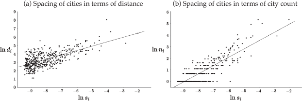
Figure 1: Spacing of Japanese cities in 2015

2.2 Size distribution of cities

It is well known that city size distribution in a well-urbanized country exhibits an approximate power law (e.g., Gabaix and Ioannides, 2004; Batty, 2006; Bettencourt, 2013). Formally, if a given set of $n$ cities is postulated to satisfy a power law, and if these city sizes are ranked as $s_{1}\geq s_{2}\geq\cdots\geq s_{n}$, so that the rank, $r_{i}$, of city $i$ is given by $r_{i}=i$, then for some positive constants $c$ and $\alpha$,

$$r_{i}/n\approx P(S>s_{i})\approx cs_{i}^{-\alpha}\Rightarrow\ln s_{i}\approx b-\frac{1}{\alpha}\ln r_{i}$$ (3)

for $b=\ln(cn)/\alpha$.

In Figure 2, Panel (a) shows the rank-size distributions of cities in every five years from 1970 to 2015, where $s_{i}$ indicates the share of city $i$ in the national population; Panel (b) shows the change in $\alpha$, i.e., the Zipf’s coefficient, over these 45 years. One can see that the city size distribution exhibits an approximate power law in each year, although agglomeration towards larger cities has been accelerated. The variation in city size is remarkably large, as exhibited by the largest three cities, Tokyo, Osaka and Nagoya, accounting for 45% of the total city population, where Tokyo alone accounts for 26% in 2015.

There is a strand of literature which informally argue that Zipf’s law (after Zipf, 1949) holds, i.e., the power law with $\alpha=1$ holds for city size distribution in a country (see, e.g., Gabaix and Ioannides, 2004; Ioannides, 2012, §8.2). But, there is abundant evidence against it (e.g., Black and Henderson, 2003; Soo, 2005; Nitsch, 2005; Mori et al., 2019), as is also clear in the Japanese case shown in Figure 2.

While the power laws for city size distributions are best known at the country level (see, e.g., Gabaix and Ioannides, 2004), Mori et al. (2019) have shown that the similar power laws appear recursively in spatial hierarchies of regions within a country that reflect the central place patterns discussed in Section 2.1. Specifically, they construct a spatial hierarchy in a country by first constructing a Voronoi partition of the set of all cities in the country using a given number of their largest cities as cell centers, and then continuing this partitioning procedure within each cell recursively. They found that city size distributions in different parts of these spatial hierarchies exhibit power laws that are significantly similar than would be expected by chance alone. Thus, their result suggests that city systems have a spatial fractal structure within countries.

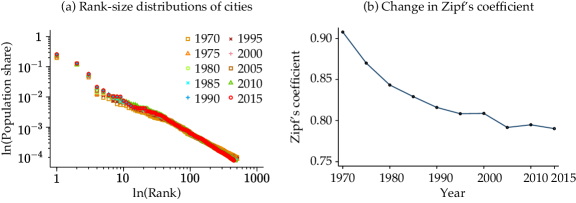
Figure 2: Rank-size distribution of cities in Japan

2.3 Size and industrial structure of cities

Many evidences (e.g. Glaeser and Maré, 2001; Bettencourt, Lobo, Helbing, Kühnert and West, 2007; Combes, Duranton and Gobillon, 2008; Glaeser and Resseger, 2010; Combes, Duranton, Gobillon, Puga and Roux, 2012; Baum-Snow and Paven, 2013; Davis and Dingel, 2019) have indicated strong correlations between socio-economic quantities and sizes of cities (e.g., wages, education level, gross domestic product, industrial diversity, number of patents applications, amount of crime, level of traffic congestion). This section presents one of the clearest representations of such correlations by focusing on industrial location.

Let $\mathcal{I}$ be the set of all industries that operate in at least one of the cities, and for a given industry $i\in\mathcal{I}$, call a city a choice city of this industry if industry $i$ is in operation in the city. These choice cities exhibit a systematic variation in their average population size across industries. To see this, denote by $\mathcal{U}_{i}\>(\subseteq\mathcal{U})$ the set of all choice cities of industry $i\in\mathcal{I}$, then the average size of choice cities for industry $i$ is given by

$$\overline{s}_{i}=\frac{1}{\#\mathcal{U}_{i}}\sum_{i\in\mathcal{U}_{i}}s_{i}\;,$$ (4)

where $\#\mathcal{U}_{i}$ means the cardinality of set $\mathcal{U}_{i}$.

Now, consider three-digit secondary and tertiary industries of the Japanese Standard Industrial Classification (JSIC) that are present both in 2000 and 2015. Of all the 237 such industries, there are 162 and 175 industries that have at least one establishment in cities in 2000 and 2015, respectively. Figure 3 shows the relationship between $\overline{s}_{i}$ and $N_{i}$ for $i\in\mathcal{I}$ in log scale, where $N_{i}\equiv\#\mathcal{U}_{i}$. The dashed curves indicate the upper and lower bound for the average size of choice cities in 2015, where for each $i\in\mathcal{I}$, the former (latter) is the average size of the largest (smallest) $N_{i}$ cities.

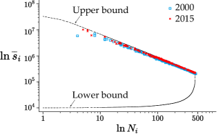
Figure 3: Varieties of economic activities and their choice of cities in Japan

There are two key features in these plots. First, the number $N_{i}$ and average size $\overline{s}_{i}$ of choice cities exhibit a strong power law, which is persistent between 2000 and 2015. Second, the average sizes of choice cities are almost hitting their upper bound, meaning that the choice cities of an industry $i\in\mathcal{I}$ is roughly the largest $N_{i}$ cities, which in turn implies that there is roughly a hierarchical relationship in the industrial composition between larger and smaller cities.

To see this, let $\mathcal{I}_{i}$ represent the set of industries that are present in city $i\in\mathcal{U}$, and for cities $i$ and $j\in\mathcal{U}$ such that $s_{i}>s_{j}$, define the hierarchy share for city $j$ with $i$ by

$$H_{ij}=\frac{\#\left(\mathcal{I}_{i}\cap\mathcal{I}_{j}\right)}{\#\mathcal{I}_{j}}\in[0,1]\;,$$ (5)

where a larger value of $H_{ij}$ indicates a higher consistency with the hierarchical relationship, and $H_{ij}=1$ means the perfect hierarchical relationship, i.e., $\mathcal{U}_{j}\subseteq\mathcal{U}_{i}$. The average values of the hierarchy shares for all the relevant city pairs,

$$H\equiv\frac{1}{\overline{H}}\sum_{i,j\in\mathcal{U}\>\>\text{s.t.}\>\>s_{i}>s_{j}}H_{ij}\>\>\in[0,1]$$ (6)

where $\overline{H}\equiv\#\{(i,j)\>:\>i,j\in\mathcal{U},\;s_{i}>s_{j}\}$, can be taken as an aggregate measure of spatial coordination among industries. A larger value of $H$ indicates a higher degree of spatial coordination, and the coordination is perfect if $H=1$. The actual values of $H$ are 0.76 and 0.80 in 2000 and 2015, respectively, which are quite high.

Together with the central place pattern discussed above (see Figure 1), the fact that the spatial coordination of diverse economic activities leads to the diversity in city size has already been suggested informally by Christaller (1933) and Lösch (1940).

A large value of $H$ as in the case of Japan above means that it is not only that industries have different number of agglomerations (i.e., choice cities), but also that their locations tend to coincide, i.e., a more localized industry choose to locate in cities in which a more ubiquitous industries are present. The case of perfect coordination (i.e., $H=1$) corresponds to the hierarchy principle in Christaller (1933).

To close this subsection, it is worth pointing out that while there is a strong tendency of hierarchical relation in the industrial composition between a larger and a smaller cities, it is by no means the rule. Figure 4 shows the distribution of $H_{ij}$ of all the relevant city pairs in 2015. While the mean value is $H=0.80$, the standard deviation is 0.13, and the range is from 0.18 to 1. Low hierarchy shares are realized for specialized cities in which only a small specific set of industries are concentrated. As will be discussed in Section 3.2, the standard systems-of-cities models (e.g., Henderson, 1974; Rossi-Hansberg and Wright, 2007) associate the size of a city with that in scale economies specific to the industries in which the city is specialized, thereby explain the diversity in city size in terms of the variation in industry-specific scale economies.

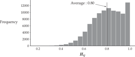
Figure 4: Distribution of hierarchy share between cities in Japan in 2015

2.4 Growth of city sizes

Finally, we look at the characteristics of the growth of individual city sizes in Japan between 1970 and 2015. It is of particular interest to quantify the evolution of city sizes in this period, since it coincides with the period in which the highway and high-speed railway networks were developed almost from scratch to the extent that covers almost the entire nation, where the total highway (high-speed railway) length increased from 879 km (515 km) by more than 16 (10) times to 14,146 km (5,350 km).

The level of interregional transport access has been one of the key parameters to determine the size and spatial patterns of cities in the literature. The evolution of the sizes of individual cities is expected to reflect the response to the improved interregional transport access, although the benefit for each city may vary depending on their relative location. Thus, the changes in size and spatial patterns experienced by Japanese cities in this period provides an ideal test case for the theoretical models of endogenous agglomeration.

There was substantial movement of population among cities in these 45 years. In particular, there is a clear tendency of global agglomeration toward a smaller number of cities, as the number of cities has decreased from 503 to 450.

Figure 5 reveals key facts about the change in individual city sizes for the 302 cities that have remained throughout the entire period. Panel (a) adds another evidence for global agglomeration: the size of the remained cities in terms of population share (in the country) has grown by 21% on average. Note that it is more meaningful to look at the population share of a city rather than the population size itself to understand the tendency of global agglomeration, because the population shares remove the effects of general population growth and/or urbanization from the population sizes.

Despite the tendency of global agglomeration, there is also a clear tendency of local dispersion as the areal size of an individual city has almost doubled (Panel, b), while the population density has decreased by 22% on average (Panel, c).

This simultaneous occurrence of global agglomeration and local dispersion given an improvement in interregional access may seem paradoxical. But, it can be explained by integrating the extant theories of endogenous agglomeration to be discussed in the next section.

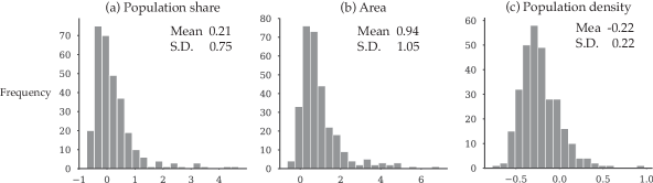
Figure 5: Changes in the sizes of individual cities in Japan between 1970 and 2015 (Growth rates in horizontarl axis)

3 Theories

A model capable of explaining the spatial patterns of cities necessarily involves many regions with large variations in interregional distance, such that some cities are close to while others are far from one another. But, the majority of the extant models adopt either two-region or systems-of-cities setups in which there is no variation in interregional distance. Thus, no explicit spatial patterns reflecting the relation among the number, size and spacing of cities can be expressed by these models.

A recent work by Akamatsu et al. (2018) brought a breakthrough by showing that a wide variety of the extant models of endogenous agglomeration can be reformulated in a many-region setup, and formally analyzed in a unified framework. Specifically, they focus on a canonical model, i.e., a static model with (i) a continuum of homogeneous mobile agents, each of whom chooses a single location; (ii) there is a single type of interregional transport cost; (iii) transport costs are subject to the iceberg technology. The reformulated models are shown to boil down to one of the three reduced forms in terms of the spatial pattern of agglomeration and dispersion.

The canonical model covers a wide range of standard models in urban and regional economics. It includes the class of NEG models based on the Dixit-Stiglitz type CES subutility function for love of variety (e.g., Krugman, 1991; Helpman, 1998; Tabuchi, 1998; Puga, 1999; Forslid and Ottaviano, 2003; Pflüger, 2004; Murata and Thisse, 2005; Redding and Sturm, 2008; Pflüger and Südekum, 2008); social-interactions model of city-center formation based on technological externalities (e.g., Beckmann, 1976; Mossay and Picard, 2011; Blanchet et al., 2016); and the economic geography models in “universal gravity” framework by Allen et al. (Forthcoming), including the Armington (1969) model with labor mobility by Allen and Arkolakis (2014), a standard formulation in the recent quantitave spatial economics (see, e.g., Redding and Rossi-Hansberg, 2017, for a survey).

Important classes of models that are out of their scope include city-center formation models in which firms and households have different location incentives (violation of (i)) (e.g., Fujita and Ogawa, 1982; Lucas and Rossi-Hansberg, 2002; Ahlfeldt et al., 2015; Monte et al., 2018); NEG models with additive transport costs (violation of (iii)) by Ottaviano et al. (2002), and those with multiple industries with industry-specific transport costs (violation of (ii)) (e.g., Fujita and Krugman, 1995; Fujita et al., 1999b; Tabuchi and Thisse, 2011).

Drawing largely from Akamatsu et al. (2018), Section 3.1 reviews the mechanism underlying the relation between population/areal size and spacing of cities in reality discussed in Sections 2.1 and 2.4. To explain the observed diversity in the size and industrial structure of cities discussed in Sections 2.2 and 2.3, respectively, and their relation to the spatial pattern of cities, a model needs to go beyond the canonical model considered by Akamatsu et al. (2018), and incorporate variations in the degree of increasing returns (and/or those in transport costs). At present, there are only a handful of models that have succeeded in such extensions. Section 3.2 reviews the theoretical development in this direction.

3.1 Spatial pattern of cities

By formalizing and generalizing the idea proposed by Krugman (1996, Ch.8) based on Turing (1952), Akamatsu, Takayama and Ikeda (2012) proposed an analytical framework for many-region models of endogenous agglomeration under the symmetric racetrack geography with the help of discrete Fourier transformation. While Akamatsu et al. (2012) has focused on a many-region extension of the model by Pflüger (2004), Akamatsu et al. (2018) have generalized their framework, and have shown that a wide variety of the extant models can be classified by the three distinct reduced forms, despite the difference in their specific mechanisms underlying agglomeration and dispersion. Below, I start by describing the basic setup of this approach.

Basic setup

Consider the location space consisting of a set of $K$ discrete regions, $\mathcal{K}\equiv\{0,1,\ldots,K-1\}$. There is a continuum of homogeneous mobile agents whose regional distribution is denoted by $\bm{h}\equiv(h_{i})_{i\in\mathcal{K}}$, where $h_{i}$ is the mass of mobile agents located in region $i$. Their total mass is a given constant, $H\equiv\sum_{i\in\mathcal{K}}h_{i}$. All regions in $\mathcal{K}$ are featureless and are placed at an equal interval on a circle. In this racetrack economy, transportation is possible only along the circumference.

Let region index $0,1,\ldots,K-1$ represent the location on the racetrack in clockwise direction. Transport costs take iceberg form, i.e., if a unit of product is shipped from region $i$ to $j$, then only the fraction $d_{ij}=d_{ji}\in[0,1)$ reaches $j$. The spatial discounting matrix, $\bm{D}=[d_{ij}]$, expresses the underlying distance structure of the economy. Typically, iceberg costs are expressed as $d_{ij}=\exp[-\tau\ell_{ij}]$, where $\ell_{ij}$ is the distance between regions $i$ and $j$ and $\tau\in(0,\infty)$ is the transport technology parameter.

The relocation of agents is assumed to be much slower than market reactions, so that the short-run equilibrium conditions (such as market clearing and trade balance) determine the payoff (utility or profit) in each region as a function of a given regional distribution of agents, $\bm{h}$. Specifically, given $\bm{h}$, their short-run payoff of choosing each region is determined, where the short-run payoff function is denoted by $\bm{v}(\bm{h})\equiv(v_{i}(\bm{h}))_{i\in\mathcal{K}}$, with $v_{i}(\bm{h})$ representing the payoff for an agent located in region $i\in\mathcal{K}$.

In the long-run, agents are mobile and are free to choose their locations to improve their own payoffs. In (long-run) equilibrium, it must hold that $v^{*}=v_{i}(\bm{h})$ for all regions $i$ with $h_{i}>0$, and $v^{*}\geq v_{i}(\bm{h})$ for any region $i$ with $h_{i}=0$, where $v^{*}$ is the equilibrium payoff level.

A change in endogenous agglomeration pattern is treated as an instance of bifurcation of an equilibrium. To address the stability of equilibria, a standard approach in the literature is to introduce equilibrium refinement based on local stability under myopic evolutionary dynamics, where the rate of change in the number of residents $h_{i}$ in region $i$ is modeled on the basis of the regional distribution of agents, $\bm{h}$, and that of payoff, $\bm{v}(\bm{h})$. Let a deterministic dynamic be denoted by $\dot{\bm{h}}=\bm{F}(\bm{h},\bm{v}(\bm{h}))$, where $\dot{\bm{h}}$ represents the time derivative of $\bm{h}$, and assume that (i) $\bm{F}$ satisfies differentiability with respect to both arguments, (ii) agents relocate in the direction of an increased aggregate payoff under $\bm{F}$, (iii) the total mass of agents is preserved under $\bm{F}$, and (iv) any spatial equilibrium is a rest point of the dynamic, i.e., if $\bm{h}^{*}$ is an equilibrium, it must hold that $\dot{\bm{h}}=\bm{F}(\bm{h}^{*},\bm{v}(\bm{h}^{*}))=\bm{0}$. The stability of an equilibrium then is defined in terms of asymptotic stability under $\bm{F}$.

Formation of a city

With a racetrack geography, the uniform distribution of mobile agents is always an equilibrium when the payoff function is symmetric across regions. Call an equilibrium with uniform distribution a flat-earth equilibrium, and denote it by $\bar{\bm{h}}\equiv(h,h,\ldots,h)$ with $h\equiv H/K$.

If the adjustment dynamic is formulated so that the agents migrate in order to maximize their payoff, it follows (Akamatsu et al., 2018, Appendix B) that each eigenvalue of Jacobian matrix $\bm{J}$ of $\bm{F}$ and that of the Jacobian matrix $\nabla\bm{v}$ of $\bm{v}$ are real, and have a perfect positive correlation at the flat-earth equilibrium. Thus, one can focus on $\nabla\bm{v}$ instead of $\bm{J}$ to investigate the stability of the flat-earth equiliburum. What remains is to identify the direction of the bifurcation at the flat-earth equilibrium, which is equivalent to find the eigenvector of $\nabla\bm{v}(\bar{\bm{h}})$ whose eigenvalue changes its sign from negative to positive first among all the eigenvectors of $\nabla\bm{v}(\bar{\bm{h}})$.

The sign of the $k$-th eigenvalue of $\nabla\bm{v}(\bar{\bm{h}})$ has been shown to coincide with the sign of the model-specific function of the form:

$$G\left(f_{k}\right)=c_{0}+c_{1}f_{k}+c_{2}f_{k}^{2},$$ (7)

where $c_{0},c_{1}$ and $c_{2}$ are the constants specific to a given model, and $f_{k}$ is the $k$-th eigenvalue of the spatial discounting matrix $\bm{D}$ which is known to be real, and common to all models. The eigenvector associated with $f_{k}$ is given by $\bm{\eta}_{k}=(\eta_{k,i})=(\cos[\theta ki])$ for $i\in\mathcal{K}$ with $\theta\equiv 2\pi/K$, and the bifurcation from the flat-earth equilibrium takes place in the direction given by $\bm{h}=\bar{\bm{h}}+\epsilon\bm{\eta}_{k}$ with $\epsilon>0$.

The value $k$ coincides with the number of equidistant regions toward which mobile agents migrate the most. For example, at $k=K/2$, the value $\eta_{K/2,i}$ of each element $i\in\mathcal{K}$ in eigenvetor, $\bm{\eta}_{K/2}$, is given as depicted for the case of $K=16$ in Figure 6(a), so that agglomerations start to form at alternate regions, $0,2,4,\ldots,K-2\,(=14)$. At $k=1$, as depicted in Figure 6(b), an unimodal agglomeration will form around region 0.

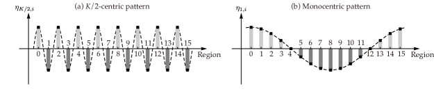
Figure 6: Agglomeration formation at high and low transport costs

There are two key properties of $f_{k}^{\prime}s$ that are useful to investigate the stability of flat-earth equilibrium:

1. $f_{k}$ is monotonically increasing in transport cost, $\tau$.

2. $f_{1}=\max_{k=1,2,\ldots,K}f_{k}$ and $f_{K/2}=\min_{k=1,2,\ldots,K}f_{k}>0$.

Canonical models typically have a positive value of $c_{1}$. Since $f_{1}>0$, it means that the second term on the right hand side (RHS) in (7) represents the agglomeration force, as it works to destabilize the flat-earth equilibrium. In these models, if a stable flat-earth equilibrium exists, then one must have either $c_{0}<0$ or $c_{2}<0$, or both, so that all the eigenvalues of $\nabla\bm{v}(\bar{\bm{h}})$ can be negative at the flat-earth equilibrium. In particular, since $f_{k}$ is positive and increasing in $\tau$ for each $k=1,2,\ldots,K-1$, the flat-earth equilibrium is stable for sufficiently small transport costs if $c_{0}<0$, and for sufficiently large transport costs if $c_{2}<0$.

The bifurcation from the flat-earth equilibrium leading to the city formation under $c_{0}<0$ and that under $c_{2}<0$ are, however, qualitatively different in two aspects. The first aspect is the timing at which the bifurcation takes place. The bifurcation under $c_{0}<0$ takes place in the increasing phase of transport costs, whereas that under $c_{2}<0$ in their decreasing phase.

The second aspect is the spatial scale of agglomeration and dispersion. Provided that $c_{2}<0$, the bifurcation takes place in the direction of $\eta_{K/2}$, i.e., every other region along the racetrack attracts in-migration of mobile agents, when $G(f_{K/2})$ becomes positive (refer to Figure 6(a)). The regional distribution of mobile agents that arises in this bifurcation is $\bar{\bm{h}}+\epsilon\bm{\eta}_{K/2}$ (for $\epsilon>0$) as illustrated in Figure 7(a). In other words, small cities (i.e., agglomerations) form locally, while they are dispersed globally all over the location space.

Provided that $c_{0}<0$, the bifurcation takes place in the direction of $\bm{\eta}_{1}$ when $G(f_{1})$ turns to positive (refer to Figure 6(b)). The regional distribution of mobile agents that arises in this case is given by $\bar{\bm{h}}+\epsilon\bm{\eta}_{1}$ as illustrated in Figure 7(b). In other words, the agglomeration takes place globally, and form a single gigantic city, while the dispersion takes place locally around the city center (region 0) so that the city stretches over the entire location space.

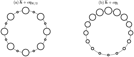
Figure 7: City formation at high and low transport costs

A crucial difference between the two cases is the dependence of dispersion force on the distance structure of the model. The third term $c_{2}f_{k}^{2}$ on the RHS of (7) depends on the distance structure of the economy (through $f_{k}$). As discussed above, this force leads to global dispersion (with local agglomeration) as in Figure 7(a). On the contrary, the first term on the RHS of (7) is the dispersion force when $c_{0}<0$ which is independent of the distance structure of the economy. As discussed above, this force leads to local dispersion (with global agglomeration) as in Figure 7(b).

In Akamatsu et al. (2018), the models with only global dispersion force, i.e., $c_{0}\geq 0$ and $c_{2}<0$, are called Class (i). The models of this class are shown to exhibit period doubling bifurcations as transport costs decrease, leading to a smaller number of larger cities with a larger spacing between neighboring cities, until all mobile agents concentrate in one region (Figure 8a). The models with only local dispersion force, i.e., $c_{0}<0$ and $c_{2}\geq 0$ are called Class (ii). The Class (ii) models involve at most one bifurcation when the flat-earth equilibrium looses stability. In the models of this class, keeping unimodal regional distribution, the concentration of mobile agents proceeds as transport costs increases, until all mobile agents concentrate in one region (Figure 8b). The models that incorporate both types of dispersion force, i.e., $c_{0}<0$ and $c_{2}<0$, may be the most realistic, and account for the formation of multiple cities with a positive internal space (Figure 8c). These are called Class (iii).

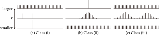
Figure 8: Spatial patterns of cities

Two implications are worth mentioning. First, the heterogeneity among interregional distances is an essential feature of a model to investigate the spatial pattern of cities. In the context of a two region model or a systems-of-cities model in which there is no variation in interregional distance, the dispersion of mobile agents in Class (i) and Class (ii) models look exactly the same. But, as indicated by the middle panels of Figure 8(a)(b), these are qualitatively different in spatial scale. The dispersion takes place at the global scale in Class (i) models – in the form of an increase in the number of cities, and at the local scale in Class (ii) models – in the form of a larger spatial extent of a city.

Second, the responses of agglomeration/dispersion to the level of transport costs are opposite between global and local spatial scales. More specifically, given the lower interregional transport costs, the agglomeration proceeds at global scale, i.e., the number of cities decreases, the sizes and the spacing of the remaining cities increase, while the dispersion proceeds at local scale, i.e., the average population density within a city decreases and the spatial extent of a city increases.

Notice that the behavior of Class (i) models essentially account for the larger cities being spaced more apart as discussed in Section 2.1, and the behavior of Class (iii) models, i.e., the combination of Classes (i) and (ii), can account for the evolution of city growth of Japan discussed in Section 2.4.

Below, I overview a variety of extant models that fall into one of these three classes, as well as those do not.

New economic geography

NEG (e.g., Fujita, Krugman and Venables, 1999a) commonly utilizes the monopolistic competition together with scale economies in production to explain the endogenous agglomeration. On the one hand, the love for product variety by consumers and the presence of transport costs give an incentive for consumers to locate closer to firms. On the other hand, each indivisible firm subject to scale economies at the plant level has an incentive to locate and supply near the concentration of consumers.

In this context, the global dispersion force associated with $c_{2}<0$ in (7) is introduced typically by assuming immobile consumers in each region who generate dispersed demand for the differentiated products (e.g., Krugman, 1991, 1993; Forslid and Ottaviano, 2003; Pflüger, 2004). The assumption of immobility of consumers is nothing but simplification to assure the dispersed demand. It can be obtained endogenously, for example, by introducing land-intensive sectors that also require labor inputs (e.g., Fujita and Krugman, 1995; Puga, 1999), which in turn generates dispersed demand from workers. With transport costs, the proximity to demand matters, and hence, the spatial dispersion of consumers results in the formation of multiple cities, where the firms in each city mainly serves their nearby local market.

The local dispersion force associated with $c_{0}<0$ in (7) is introduced by assuming consumption of locally scarce land (e.g., Helpman, 1998; Redding and Sturm, 2008; Redding and Rossi-Hansberg, 2017), sometimes together with commuting costs (e.g., Murata and Thisse, 2005). All these costs of concentration are confined within a given region, and thus are independent of interregional distance. The dispersion in this case takes the form of overflow of mobile agents from a given city to the nearby regions, rather than the formation of new distinct cities at distant regions.

There are models that incorporate both global and local dispersion forces above (Tabuchi, 1998; Pflüger and Südekum, 2008), i.e., of Class (iii) with $c_{0}<0$ and $c_{2}<0$ in (7). While these themselves treat only the two-region case, their many-region extensions can generate a more realistic spatial pattern of cities that involve both global and local dispersion as shown in Figure 8(c) (see Akamatsu et al., 2018, §5.3).

Social interactions model

In the 1970s and 1980s, there were a series of attempts to explain endogenous formation of the central business districts (CBD) within a city. The development of the models of this type was initiated by Solow and Vickrey (1971) and Beckmann (1976), then followed by several others (e.g., Borukhov and Hochman, 1977; O’Hara, 1977; Ogawa and Fujita, 1980; Fujita and Ogawa, 1982; Imai, 1982; Tauchen and Witte, 1983; Tabuchi, 1986; Fujita, 1988; Kanemoto, 1990; Fujita, 1990).

In these models, the formation of CBD is explained by introducing positive technological externalities generated from the interaction between each pair of individual agents. While the above mentioned models vary in the specification of positive externalities, Fujita and Smith (1990) have shown that their formulations are essentially equivalent, and reformulated commonly by the so-called additive interaction function, $S_{i}(\bm{h})\equiv\sum_{j\in\mathcal{K}}d_{ij}h_{j}$.

In the simplest specifications (as in, e.g., Beckmann, 1976), this additive interaction function enters the utility function of consumers directly. Most models assume land consumption by mobile agents, while the production sector is abstracted, i.e., they incorporate only local dispersion force, and hence belong to Class (ii). One exception is Takayama and Akamatsu (2011) who also included global dispersion force by introducing mobile firms and immobile consumers in each region. This model thus contains both local and global dispersion force, i.e., of Class (iii).

Other relevant models

In the NEG literature, a particularly important deviation from the canonical models is to consider different transport cost structures by industry. For example, Fujita and Krugman (1995) included transport costs for (urban) differentiated products as well as land-intensive (rural) homogenous products. In the presence of rural goods that are costly to transport, the delivered price for such goods is lower in regions farther away from cities, which generates a dispersion force. This is similar to the local dispersion force in that even a small deviation from an urban agglomeration will decrease the price of rural goods and increase the payoff of the deviant. However, the advantage of dispersion persists outside the agglomeration, i.e., it depends on the distance structure of the model. This type of dispersion force has been shown to result in the formation of an industrial belt, a continuum of agglomeration associated with multiple atoms of agglomeration as demonstrated by the simulations in Mori (1997) and Ikeda, Murota, Akamatsu and Takayama (2017). The formal characterization of industrial belts, however, remains to be carried out.

Among the extant social-interactions models, some distinguish location incentives between firms and consumers/workers unlike the canonical models discussed above (e.g., Ogawa and Fujita, 1980; Fujita and Ogawa, 1982; Ota and Fujita, 1993; Lucas and Rossi-Hansberg, 2002). This distinction is especially crucial for explaining the location patterns within a city, while it may be less relevant for the purpose of explaining the spatial pattern of cities. At present, little formal results have been obtained regarding the spatial pattern of cities that arise in these models (see Osawa, 2016, for the recent theoretical development in this direction.)

Other relevant models that were not covered so far include the spatial oligopoly models designed to explain the agglomeration of retail stores (e.g., Wolinsky, 1983; Dudey, 1990; Konishi, 2005). In these models, consumers have imperfect information on the types and prices of goods sold by stores before they visit them. The greater the agglomeration of stores, the more likely it is that consumers will find their favorite commodities. The concentration of stores is explained by the market-size effect due to taste uncertainty and/or lower price expectation. The dispersion force is global one given by the exogenous and spatially dispersed demand. Thus, these models are expected to behave similarly to Class (i) models above, although no extensive analyses have been conducted in this direction (see Konishi, 2005, §5, for the discussion on the spacing of retail clusters).

3.2 Diversity in city size

The most popular theoretical explanation of power law for city-size distribution at this point may be the random growth theory (e.g., Gabaix, 1999; Duranton, 2006, 2007; Rossi-Hansberg and Wright, 2007; Ioannides, §8.2, 2012) which postulates that the growth rates of individual cities follows Gibrat’s law (Gibrat, 1931), i.e., they are independently and identically distributed random variables.

This theory is highly compatible with systems-of-cities models. For example, in the model by Rossi-Hansberg and Wright (2007), individual industries are subject to city-level positive externality from agglomeration, but do not benefit from colocation with other industries, so that the externality is industry-specific. Then, each city would specialize in a single industry in the presence of urban costs due to scarcity of land and the need for commuting in a city. If the industry- (or city-) specific productivity growth rates satisfy the basic assumptions of random growth theory (including Gibrat’s law), the model generates the power law for city size distributions. It is a plausible explanation, as we have seen in Section 2.3 that the specialized cities are rather ubiquitous (refer to Figure 4 and the corresponding discussion) despite the strong evidence for the hierarchy principle à la Christaller (1933).

A key implication of the random growth theory is that similar power laws hold for all (sufficiently large) random subsets of cities in a country, i.e., without any regard to spatial relation among cities. Thus, this theory essentially denies the mutual dependence of size and spatial patterns of cities. But, as discussed in Section 2.2, Mori et al. (2019) have shown that the similarity in power laws for city size distributions is much stronger among the cells in the spatial hierarchical partitions of cities that are consistent with the central place patterns than among random subsets of cities, i.e., if city sizes were generated by a random growth process.

To account for the large diversity in city size observed in reality by the many-region models described in Section 3.1, one needs to incorporate diversity in increasing returns (and/or that in transport costs). While Class (i) models with a global dispersion force discussed above can account for the formation of multiple cities, there is little variation in the sizes of cities to be realized in equilibrium, since each model has only one type of increasing returns.

There has been attempts of formalizing the central place thoery of Christaller (1933) by introducing multiple industries subject to different degrees of increasing returns. The initial formal attempt was made by Beckmann (1958). But, his model lacked microeconomic foundation. Later the models with more explicit mechanisms were developed by Fujita, Krugman and Mori (1999b); Tabuchi and Thisse (2011) in the context of the NEG, and by Hsu (2012) in the context of spatial competition model. In these models, the different degrees of increasing returns among industries result in the different spatial frequencies of agglomeration among industries.

The key to account for the diversity in city size in these models is the spatial coordination of agglomerations among industries through inter-industry demand externalities that arise from common consumers among industries. An industry subject to a larger increasing returns agglomerate in a smaller number of cities that are farther apart. What is crucial is that these cities are chosen from the ones in which more ubiquitous industries subject to smaller increasing returns are located. Consequently, larger cities are formed at the location in which the coordination of a larger number of industries takes place. This spatial coordination of industries accounts for the positive correlation between the size, spacing and industrial diversity of a city as observed in reality (Sections 2.1 and 2.3).

In particular, Hsu (2012) proposed a unique spatial competition model with product differentiation and scale economies in production, and provided at this point the most far reaching formal explanation for the mutual dependence between spatial pattern and size diversity of cities. When the distribution of scale economies in production of each firm (which is expressed in terms of the industry-specific fixed cost for production in his model) is regularly varying, then his model replicates the power law for city size distribution (Section 2.2) together with the positive correlation between size and spacing of cities (Section 2.1), the power law for the number and the average size of choice cities of industries (Section 2.3), as well as the hierarchy principle observed in Japan (Section 2.3).

Davis and Dingel (2019) offer an alternative mechanism of spatial coordination among industries which in turn results in hierarchy principle and the diversity in city sizes in the context of a systems-of-cities model. Specifically, the hierarchy principle in this model arises from vertical heterogeneity in skill level among workers and skill requirement by industries together with inter-industry positive externality that is confined within the same city. The mechanism underling the spatial coordination among industries in this model is different from the central place models above. On the one hand, a small city attracts only low skill industries and workers as it offers only small city-level agglomeration externality. On the other hand, a large city attracts both high and low skill industries and workers. High skilled have an incentive to live there, since the city offers a large city-level agglomeration externality and they can afford to live there. Although residential locations near the city center are occupied by high skilled, low skilled still can afford to live in locations with low land rent (due to longer commuting) near the city fringe, while enjoying the large city-level externality.

Alternatively, Desmet and Rossi-Hansberg (2009), Desmet and Rossi-Hansberg (2014), Desmet and Rossi-Hansberg (2015), Desmet et al. (2017) incorporated dynamic externalities through endogenous innovation and spillover effects. These models are fundamentally different from all the models discussed so far in that the exogenous heterogeneity among regions are essential for city formation, i.e., agglomerations do not form spontaneously. The uneven distribution of mobile agents resulting from the exogenous regional heterogeneity is magnified by the spillover effects over time. One exception in this strand of literature is Nagy (2017) who incorporated the same dynamic externalities into the NEG framework, so that his model is capable of explaining the spontaneous formation of multiple cities together with the diversity in city sizes. While this model has been applied to replicate the evolution of the US cities in 19th century, the properties of agglomeration and dispersion in this model have not been formally analyzed.

4 Concluding remarks

This paper reviewed the models which explain the mutual dependence of spatial pattern and sizes of cities. A many-region geography with variations in interregional distance is an essential feature of a model, if the spatial pattern of cities were the subject of the study. Naturally, there have been very few formal attempts that explicitly dealt with this high-dimensional problem until recently with notable exceptions by Hsu (2012).

A breakthrough has been brought about by Akamatsu et al. (2012) who proposed to focus on the racetrack economy which involves many regions with heterogeneous interregional distances, while preserving symmetry among the regions. By utilizing the discrete Fourier transformation, they have demonstrated that the spatial patterns of agglomeration that aries in the NEG models in a many region setup can be formally analyzed to a large extent. The same group of researchers have also developed the framework for systematic numerical analysis on a many-region geography based on the numerical bifurcation theory and group-theoretic bifucation theory (e.g., Ikeda, Akamatsu and Kono, 2012; Ikeda et al., 2017). Their numerical approach makes it possible to explore asymmetric geography (e.g., the presence of edges and heterogeneity in regional advantages) as well as two-dimensional location space in a many-region setup.

In this paper, drawing largely from Akamatsu et al. (2018) which applied the analytical tool developed by Akamatsu et al. (2012) to a wide variety of extant agglomeration models, I have reviewed the spatial pattern of cities and its relation to city sizes implied by these models. But, Hsu (2012) continues to be the only tractable model that can account for the large diversity in city size in association with the observed spatial pattern of cities. Thus, much to be expected in the future development in this respect.

Finally, no models so far have been successful in integrating intra- and inter-city space. In the models aiming to explain intra-city spatial patterns, the location behavior of firms and that of workers are typically distinguished, and land consumption and/or land inputs by firms together with commuting are considered (e.g., Fujita and Ogawa, 1982; Ota and Fujita, 1993; Lucas and Rossi-Hansberg, 2002; Picard and Tabuchi, 2013). The models aiming to explain inter-city spatial patterns, on the contrary, typically ignore different location incentives between firms and workers (all models discussed in this paper belong to this group). But, it is not trivial to integrate these two spatial scales in one model.

Some extant NEG models consider commuting and land consumption (e.g., Anas, 2004; Murata and Thisse, 2005). But, such urban structure is by assumption confined within a given region, and does not extend beyond a single region. As is discussed in Section 3.1, in a many-region geography with variations in interregional distance, these models belong to Class (ii), which means that at most unimodal agglomeration forms. Although each region in these models has monocentric urban structure by assumption, and hence, it is tempted to be interpreted as a “city”, they can generate essentially at most one “true” city.

To fully account for the spatial pattern of cities, the distinction between inside and outside each city should also be endogenized.

References

- (1)
- Abdel-Rahman and Anas (2004) Abdel-Rahman, Hesham M. and Alex Anas, Theories of systems of cities, 1 ed., Vol. 4 of Handbook of Regional and Urban Economics, Amsterdam: Elsevier,
- Ahlfeldt et al. (2015) Ahlfeldt, Gabriel M., Stephen J. Redding, Daniel M. Sturm, and Nikolaus Wolf, “The economics of density: Evidence from the Berlin Wall,” Econometrica, November 2015, 83 (6), 2127–2189.
- Akamatsu et al. (2018) Akamatsu, Takashi, Tomoya Mori, Minoru Osawa, and Yuki Takayama, “Spatial scale of agglomeration and dispersion: Theoretical foundations and empirical implications,” January 2018. Disussion Paper No. 84145, Munich Personal RePEc Archives.
- Akamatsu et al. (2012) , Yuki Takayama, and Kiyohiro Ikeda, “Spatial discounting, Fourier, and racetrack economy: A recipe for the analysis of spatial agglomeration models,” Journal of Economic Dynamics & Control, 2012, 36, 1729–1759.
- Allen and Arkolakis (2014) Allen, Treb and Costas Arkolakis, “Trade and the topography of the spatial economy,” The Quarterly Journal of Economics, 2014, 129 (3), 1085–1140.
- Allen et al. (Forthcoming) , , and Yuta Takahashi, “Universal gravity,” Journal of Political Economy, Forthcoming.
- Alonso (1964) Alonso, William, Location and Land Use, Cambridge, MA: Harvard University Press, 1964.
- Anas (2004) Anas, Alex, “Vanishing cities: What does the new economic geography imply about the efficiency of urbanization?,” Journal of Economic Geography, April 2004, 4 (2), 181–199.
- Anas and Xiong (2003) and Kai Xiong, “Intercity trade and the industrial diversification of cities,” Journal of Urban Economics, 2003, 54 (2), 258–276.
- Armington (1969) Armington, Paul S., “A theory of demand for product distinguished by place of production,” International Monetary Fund Staff Papers, 1969, 16 (1), 159–178.
- Baldwin et al. (2003) Baldwin, Richard, Rikard Forslid, Philippe Martin, Gianmarco I.P. Ottaviano, and Frederic Robert-Nicoud, Economic Geography and Public Policy, Princeton, NJ: Princeton University Press, 2003.
- Batty (2006) Batty, Michael, “Rank clocks,” Nature, 2006, 444, 592–596.
- Baum-Snow (2007) Baum-Snow, Nathaniel, “Did highways cause suburbanization?,” The Quarterly Journal of Economics, May 2007, 122 (2), 775–805.
- Baum-Snow (2017) , “Urban transport expansions, employment decentralization, and the spatial scope of agglomeration economies,” 2017. Unpublished manuscript.
- Baum-Snow and Paven (2013) and Ronni Paven, “Inequality and city size,” Review of Economics and Statistics, December 2013, 95 (5), 1535–1548.
- Beckmann (1976) Beckmann, Martin, Mathematical Land Use Theory, Lexington, MA: Lexington Books,
- Beckmann (1958) Beckmann, Martin J., “City hierarchies and the distribution of city size,” Economic Development and Cultural Change, 1958, 6 (3), 243–248.
- Behrens and Robert-Nicoud (2015) Behrens, Kristian and Frederic Robert-Nicoud, “Agglomeration theory with heterogeneous agents,” in Gilles Duranton, J. Vernon Henderson, and William C. Strange, eds., Handbook of Regional and Urban Economics, Vol. 5, Elsevier, 2015, pp. 171–245.
- Bettencourt (2013) Bettencourt, Luís M. A., “The origins of scaling in cities,” Science, 2013, 340, 1438–1441.
- Bettencourt et al. (2007) , José Lobo, Dirk Helbing, Cristian Kühnert, and Geoffrey B. West, “Growth, innovation, scaling, and the pace of life in cities,” Proceedings of the National Academy of Sciences of the United States of America, 2007, 104 (7), 7301–7306.
- Black and Henderson (2003) Black, Duncan and J. Vernon Henderson, “Urban evolution in the USA,” Journal of Economic Geography, 2003, 3 (4), 343–372.
- Blanchet et al. (2016) Blanchet, Adrien, Pascal Mossay, and Filippo Santambrogio, “Existence and uniqueness of equilibrium for a spatial model of social interactions,” International Economic Review, 2016, 57 (1), 36–60.
- Bleakley and Lin (2012) Bleakley, Hoyt and Jeffrey Lin, “Portage and path dependence,” The Quarterly Journal of Economics, 2012, 127, 587–644.
- Borukhov and Hochman (1977) Borukhov, Eli and Oded Hochman, “Optimum and market equilibrium in a model of a city without a predetermined center,” Environment and Planning A, 1977, 9 (8), 849–856.
- Christaller (1933) Christaller, Walter, Die Zentralen Orte in Süddeutschland, Jena: Gustav Fischer, 1933.
- Combes et al. (2008) Combes, Pierre-Philippe, Gilles Duranton, and Laurent Gobillon, “Spatial wage disparities: Sorting matters!,” Journal of Urban Economics, March 2008, 63 (2), 723–742.
- Combes et al. (2012) , , , Diego Puga, and Sébastien Roux, “The productivity advantage of large cities: Distinguishing agglomeration from firm selection,” Econometrica, November 2012, 80 (6), 2543–2594.
- Cronon (1991) Cronon, William, Nature’s Metropolis: Chicago and the Great West, New York: W. W. Norton & Company, 1991.
- Davis and Weinstein (2002) Davis, Donald R. and David E. Weinstein, “Bones, bombs, and break points: The geography of economic activity,” American Economic Review, December 2002, 92 (5), 1269–1289.
- Davis and Dingel (2019) and Jonathan I. Dingel, “The comparative advantage of cities,” April 2019. Unpublished manuscript, The University of Chicago Booth School of Business.
- Desmet and Rossi-Hansberg (2009) Desmet, Klaus and Esteban Rossi-Hansberg, “Spatial growth and industry age,” Journal of Economic Theory, 2009, 144 (6), 2477–2502s.
- Desmet and Rossi-Hansberg (2014) and , “Spatial development,” American Economic Review, 2014, 104 (4), 1211–1243.
- Desmet and Rossi-Hansberg (2015) and , “The spatial development of India,” Journal of Regional Science, 2015, 55 (1), 10–30.
- Desmet et al. (2017) , Dávid Krisztián Nagy, and Esteban Rossi-Hansberg, “The geography of development,” Journal of Political Economy, 2017, forthcoming.
- Dittmar (2011) Dittmar, Jeremiah, “Cities, markets, and growth: The emergence of Zipf’s law,” 2011. Unpublished manuscript, London Shool of Econoimcs.
- Dobkins and Ioannides (2001) Dobkins, Linda Harris and Yannis M. Ioannides, “Spatial interactions among U.S. cities: 1900-1990,” Regional Science and Urban Economics, 2001, 31 (6), 701–731.
- Dudey (1990) Dudey, Marc, “Competition by choice: The effect of consumer search on firm location decisions,” American Economic Review, December 1990, 80 (5), 1092–1104.
- Duranton (2006) Duranton, Gilles, “Some foundations for Zipf’s law: Product proliferation and local spillovers,” Regional Science and Urban Economics, July 2006, 36 (4), 542–563.
- Duranton (2007) , “Urban evolutions: The fast, the slow and the still,” American Economic Review, 2007, 97 (1), 197–221.
- Duranton and Turner (2012) and Matthew A. Turner, “Urban growth and transportation,” Review of Economic Studies, 2012, 79 (4), 1407–1440.
- Economides and Siow (1988) Economides, Nicholas and Aloysius Siow, “The division of markets is limited by the extent of liqidity (Spatial competition with externalities),” American Economic Review, March 1988, 78 (1), 108–121.
- Faber (2014) Faber, Benjamin, “Trade integration, market size, and industrialization: Evidence from China’s national trunk highway system,” Review of Economic Studies, 2014, 81 (3), 1046–1070.
- Forslid and Ottaviano (2003) Forslid, Rikard and Gianmarco I.P. Ottaviano, “An analytically solvable core-periphery model,” Journal of Economic Geography, 2003, 3, 229–240.
- Fujita (1988) Fujita, Masahisa, “A monopolistic competition model of spatial agglomeration: Differentiated product approach,” Regional Science and Urban Economics, 1988, 18, 87–124.
- Fujita (1990) , “Spatial interactions and agglomeration in urban economics,” in M. Chatterji and R.E. Kune, eds., New Frontiers in Regional Science, London: Macmillan Publishers, 1990, chapter 12, pp. 184–221.
- Fujita (2010) , “The evolution of spatial economics: From Thünen to the new economic geography,” The Japanese Economic Review, March 2010, 61 (1), 1–32.
- Fujita (2012) , “Thünen and the new economic geography,” Regional Science and Urban Economics, 2012, 42 (6), 907–912.
- Fujita and Ogawa (1982) and Hideaki Ogawa, “Multiple equilibria and structural transformation of non-monocentric urban configurations,” Regional Science and Urban Economics, 1982, 12, 161–196.
- Fujita and Krugman (1995) and Paul Krugman, “When is the economy monocentric?: von Thünen and Chamberlin unified,” Regional Science and Urban Economics, August 1995, 25 (4), 505–528.
- Fujita and Mori (1997) and Tomoya Mori, “Structural stability and evolution of urban systems,” Regional Science and Urban Economics, August 1997, 27 (4-5), 399–442.
- Fujita and Smith (1990) and Tony E. Smith, “Additive-interaction models of spatial agglomeration,” Journal of Regional Science, 1990, 30 (1), 51–74.
- Fujita et al. (1999a) , Paul Krugman, and Anthony J. Venables, The Spatial Economy: Cities, Regions, and International Trade, Cambridge, Massachusetts: The MIT Press, 1999.
- Fujita et al. (1999b) , , and Tomoya Mori, “On the evolution of hierarchical urban systems,” European Economic Review, 1999, 43, 209–251.
- Gabaix (1999) Gabaix, Xavier, “Zipf’s law for cities: An explanation,” The Quarterly Journal of Economics, 1999, 114 (3), 738–767.
- Gabaix and Ioannides (2004) and Yannis M. Ioannides, “The evolution of city size distributions,” in J. Vernon Henderson and Jacques-François Thisse, eds., Handbook of Regional and Urban Economics, Vol. 4, Elsevier, 2004, chapter 53, pp. 2341–2378.
- Ottaviano et al. (2002) Gianmarco, I.P. Ottaviano, Takatoshi Tabuchi, and Jacques-François Thisse, “Agglomeration and trade revisited,” International Economic Review, 2002, 43, 403–436.
- Gibrat (1931) Gibrat, Robert, Les Inégalité Économiques, Paris: Librairie du Recueil Sirey, 1931.
- Glaeser and Maré (2001) Glaeser, Edward L. and David C. Maré, “Cities and skills,” Journal of Labor Economics, 2001, 19 (2), 316–342.
- Glaeser and Resseger (2010) and Matthew G. Resseger, “The complementarity between cities and skills,” Journal of Regional Science, 2010, 50 (1), 221–244.
- Helpman (1998) Helpman, Elhanan, “The size of regions,” in D. Pines, E. Sadka, and I. Zilcha, eds., Topics in Public Economics: Theoretical and Applied Analysis, Cambridge University Press, 1998, pp. 33–54.
- Henderson (1974) Henderson, J. Vernon, “The sizes and types of cities,” American Economic Review, September 1974, 64 (4), 640–656.
- Hsu (2012) Hsu, Wen-Tai, “Central place theory and city size distribution,” The Economic Journal, 2012, 122, 903–932.
- Huber and Rust (2016) Huber, Stephan and Christoph Rust, “Calculate travel time and distance with OpenStreetMap data using Open Source Routing Machine (OSRM),” Stata Journal, June 2016, 16 (2), 416–423.
- Ikeda et al. (2017) Ikeda, Kiyohiro, Kazuo Murota, Takashi Akamatsu, and Yuki Takayama, “Agglomeration patterns in a long narrow economy of a new economic geography model: Analogy to a racetrack economy,” International Journal of Economic Theory, 2017, 13, 113–145.
- Ikeda et al. (2012) Ikeda, Kyohiro, Takashi Akamatsu, and Tatsuhito Kono, “Spatial period-doubling agglomeration of a core-periphery model with a system of cities,” Journal of Economic Dynamics & Control, 2012, 36 (5), 754–778.
- Imai (1982) Imai, Haruo, “CBD hypothesis and economies of agglomeration,” Journal of Economic Theory, 1982, 28, 275–299.
- Ioannides (2012) Ioannides, Yannis, From Neighborhoods to Nations: The Economics of Social Interactions, Princeton, NJ: Princeton University Press, 2012.
- Ioannides and Overman (2004) Ioannides, Yannis M. and Henry G. Overman, “Spatial evolution of the US urban system,” Journal of Economic Geography, 2004, 4 (2), 131–156.
- Isard (1949) Isard, Walter, “The General Theory of Location and Space-Economy,” The Quarterly Journal of Economics, 1949, 63 (4), 476–506.
- Isard (1956) , Location and Space-Economy, Cambridge, MA: The MIT Press, 1956.
- Kanemoto (1990) Kanemoto, Yoshitsugu, “Optimal cities with indivisibility in production and interactions between firms,” Journal of Urban Economics, 1990, 27 (1), 46–59.
- Konishi (2005) Konishi, Hideo, “Concentration of competing retail stores,” Journal of Urban Economics, 2005, 58 (3), 651–667.
- Krugman (1991) Krugman, Paul, “Increasing returns and economic geography,” Journal of Political Economy, 1991, 99, 483–499.
- Krugman (1993) , “On the number and location of cities,” European Economic Review, 1993, 37, 293–298.
- Krugman (1996) Krugman, Paul R., The Self-Organizing Economy, Cambridge, MA: Blackwell, 1996.
- Lösch (1940) Lösch, August, Die räumliche Ordnung der Wirtschaft, Jena: Gustav Fischer, 1940.
- Lucas and Rossi-Hansberg (2002) Lucas, Robert E. and Esteban Rossi-Hansberg, “On the internal structure of cities,” Econometrica, 2002, 70 (4), 1445–1476.
- Michaels and Rauch (2018) Michaels, Guy and Ferdinand Rauch, “Resetting the urban network: 117-2012,” Economic Journal, 2018, 138 (608), 378–412.
- Monte et al. (2018) Monte, Ferdinando, Stephen J. Redding, and Esteban Rossi-Hansberg, “Commuting, migration and local employment,” American Economic Review, 2018, 108 (12), 3855–3890.
- Mori (1997) Mori, Tomoya, “A modeling of megalopolis formation: the maturing of city systems,” Journal of Urban Economics, 1997, 42, 133–157.
- Mori (2017) , “Evolution of the size and industrial structure of cities in Japan between 1980 and 2010: Constant churning and persistent regularity,” Asian Development Review, 2017, 34 (2), 86–113.
- Mori and Smith (2011) and Tony E. Smith, “An industrial agglomeration approach to central place and city size regularities,” Journal of Regional Science, 2011, 51 (4), 694–731.
- Mori et al. (2008) , Koji Nishikimi, and Tony E. Smith, “The number-average size rule: A new empirical relationship between industrial location and city size,” Journal of Regional Science, 2008, 48 (1), 165–211.
- Mori et al. (2019) , Tony E. Smith, and Wen-Tai Hsu, “Cities and space: Common power laws and spatial fractal structures,” 2019. Discussion paper, arXiv:1907.12289.
- Mossay and Picard (2011) Mossay, Pascal and Pierre M. Picard, “On spatial equilibria in a social interaction model,” Journal of Economic Theory, 2011, 146 (6), 2455–2477.
- Murata and Thisse (2005) Murata, Yasusada and Jacques-François Thisse, “A simple model of economic geography à la Helpman-Tabuchi,” Journal of Urban Economics, 2005, 58 (1), 135–155.
- Nagy (2017) Nagy, Dávid Krisztián, “City location and economic growth,” January 2017. Unpublished manuscript.
- Nitsch (2005) Nitsch, Volker, “Zipf zipped,” Journal of Urban Economics, 2005, 57 (1), 86–100.
- Oak Ridge National Laboratory (2015) Oak Ridge National Laboratory, “LandScan,” 2015. UT-Battelle, LLC, operator of Oak Ridge National Laboratory under Contract No. DE-AC05-00OR22725 with the US Department of Energy.
- Ogawa and Fujita (1980) Ogawa, Hideaki and Masahisa Fujita, “Equilibrium land use patterns in a nonmonocentric city,” Journal of Regional Science, 1980, 20 (4), 455–475.
- O’Hara (1977) O’Hara, Donald J., “Location of firms within a square central business district,” Journal of Political Economy, December 1977, 85 (6), 1189–1207.
- Osawa (2016) Osawa, Minoru, “Monocentric and polycentric patterns in the spatial economy: A unification of intra-city and inter-regional theories.” PhD dissertation, Graduate School of Information Sciences, Tohoku University 2016.
- Ota and Fujita (1993) Ota, Mitsuru and Masahisa Fujita, “Communication technologies and spatial organization of multi-unit firms in metropolitan areas,” Regional Science and Urban Economics, 1993, 23 (6), 695–729.
- Overman and Ioannides (2001) Overman, Henry G. and Yannis M. Ioannides, “Cross-sectional evolution of the U.S. city size distribution,” Journal of Urban Economics, 2001, 49 (3), 543–566.
- Pflüger (2004) Pflüger, Michael, “A simple, analytically solvable, Chamberlinian agglomeration model,” Regional Science and Urban Economics, 2004, 34 (5), 565–573.
- Pflüger and Südekum (2008) and Jens Südekum, “Integration, agglomeration and welfare,” Journal of Urban Economics, March 2008, 63 (2), 544–566.
- Picard and Tabuchi (2013) Picard, Pierre M. and Takatoshi Tabuchi, “On microfoundations of the city,” Journal of Economic Theory, 2013, 148 (6), 2561–2582.
- Puga (1999) Puga, Diego, “The rise and fall of regional inequalities,” European Economic Review, 1999, 43 (2), 303–334.
- Redding and Sturm (2008) Redding, Stephen J. and Daniel Sturm, “The cost of remoteness: Evidence from German division and reunification,” American Economic Review, 2008, 98 (5), 1766–1797.
- Redding and Rossi-Hansberg (2017) and Esteban Rossi-Hansberg, “Quantitative spatial economics,” Annual Review of Economics, 2017, 9, 21–58.
- Rosenfeld et al. (2011) Rosenfeld, Hernán D., Diego Rybski, Xavier Gabaix, and Hernán A. Makse, “The area and populaation of cities: New insights from a different perspective on cities,” American Economic Review, August 2011, 101 (5), 2205–2225.
- Rossi-Hansberg and Wright (2007) Rossi-Hansberg, Esteban and Mark L. J. Wright, “Urban structure and growth,” Review of Economic Studies, 2007, 74 (2), 597–624.
- Rozenfeld et al. (2008) Rozenfeld, Hernán D., Diego Rybski, Jr. José S. Andrade, Michael Batty, H. Eugene SWtanley, and Hernán A. Makse, “Laws of population growth,” Proceedings of the National Academy of Sciences of the United States of America, December 2008, 105 (48), 18702–18707.
- Rybski and Ros (2013) Rybski, Diego and Anselmo García Cantú Ros, “Distance-weighted city growth,” Physical Review E, 2013, 87 (042114), 1–6.
- Schiff (2014) Schiff, Nathan, “Cities and product variety: Evidence from restaurants,” Journal of Economic Geography, 2014, 15 (6), 1085–1123.
- Solow and Vickrey (1971) Solow, Robert M. and William S. Vickrey, “Land use in a long narrow city,” Journal of Economic Theory, December 1971, 3 (4), 430–447.
- Soo (2005) Soo, KwokTong, “Zipf’s law for cities: a cross country investigation,” Regional Science and Urban Economics, 2005, 35 (3), 239–263.
- Statistics Bureau, Ministry of Internal Affairs and Communication of Japan (2001) Statistics Bureau, Ministry of Internal Affairs and Communication of Japan, “The Establishment and Enterprise Census,” 2001.
- Statistics Bureau, Ministry of Internal Affairs and Communication of Japan (2014) , “Economic Census for Business Frame,” 2014.
- Statistics Bureau, Ministry of Internal Affairs and Communication of Japan (2015) , “Population Census (Tabulation for standard area mesh),” 2015.
- Tabuchi (1986) Tabuchi, Takatoshi, “Urban agglomeration economies in a linear city,” Regional Science and Urban Economics, August 1986, 16 (3), 421–436.
- Tabuchi (1998) , “Urban agglomeration and dispersion: A synthesis of Alonso and Krugman,” Journal of Urban Economics, 1998, 44 (3), 333–351.
- Tabuchi and Thisse (2011) and Jacques-François Thisse, “A new economic geography model of central places,” Journal of Urban Economics, 2011, 69 (2), 240–252.
- Tabuchi et al. (2005a) , , and Dao-Zhi Zeng, “On the number and size of cities,” Journal of Economic Geography, 2005, 5 (4), 423–448.
- Tabuchi et al. (2005b) , , and Dao-Zi Zeng, “On the number and size of cities,” Journal of Economic Geography, 2005, 5, 423–448.
- Takayama and Akamatsu (2011) Takayama, Yuki and Takashi Akamatsu, “Emergence of polycentric urban configurations from combination of communication externality and spatial competition,” Journal of JSCE Series D3: Infrastructure Planning and Management, 2011, 67 (1), 001–020.
- Tauchen and Witte (1983) Tauchen, Helen and Ann D. Witte, “An equilibrium model of office location and contact patterns,” Environment and Planning A, February 1983, 15 (10), 1311–1326.
- Thisse et al. (1996) Thisse, Jacques-François, Kenneth J. Button, and Peter Nijkamp (eds.), Location Theory, Vol. I& II of Modern Classics in Regional Science, Brookfield, VT: Edward Elger, 1996.
- Turing (1952) Turing, Alan M., “The chemical basis of morphogenesis,” Philosophical Transactions of the Royal Society, 1952, 237 (641), 37–72.
- von Thünen (1826) von Thünen, Johann Heinrich, Der Isolierte Staat in Beziehung auf Landwirtschaft und Nationalökonomie, Hamburg, Perthes. English translation by C.M. Wartenberg: von Thünen’s Isolated State, Oxford: Pergammon Press (1966), 1826.
- Wolinsky (1983) Wolinsky, Asher, “Retail trade concentration due to consumers’ imperfect information,” The Bell Journal of Economics, Spring 1983, 14 (1), 275–282.
- Zipf (1949) Zipf, George K., Human Behavior and the Principle of Least Effort, Cambridge, MA: Addison-Wesley, 1949.