Asynchronous Single-Photon 3D Imaging

Abstract

Single-photon avalanche diodes (SPADs) are becoming popular in time-of-flight depth-ranging due to their unique ability to capture individual photons with picosecond timing resolution. However, ambient light (e.g., sunlight) incident on a SPAD-based 3D camera leads to severe non-linear distortions (pileup) in the measured waveform, resulting in large depth errors. We propose asynchronous single-photon 3D imaging, a family of acquisition schemes to mitigate pileup during data acquisition itself. Asynchronous acquisition temporally misaligns SPAD measurement windows and the laser cycles through deterministically predefined or randomized offsets. Our key insight is that pileup distortions can be “averaged out” by choosing a sequence of offsets that span the entire depth range. We develop a generalized image formation model and perform theoretical analysis to explore the space of asynchronous acquisition schemes and design high-performance schemes. Our simulations and experiments demonstrate an improvement in depth accuracy of up to an order of magnitude as compared to the state-of-the-art, across a wide range of imaging scenarios, including those with high ambient flux.

1 Single-Photon Cameras

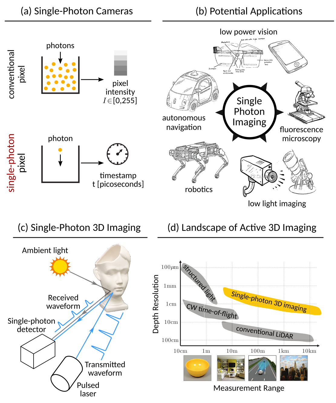
Figure 1: Single-photon cameras and 3D imaging. (a) A single-photon camera pixel is sensitive to individual photons and can capture photon arrival times with picosecond resolution. (b) The extreme sensitivity and resolution makes single-photon cameras promising candidates for several applications. (c) A single-photon 3D camera based on time-of-flight consists of a pulsed laser and a single-photon detector that timestamps returning photons. (d) Single-photon 3D cameras have the potential to provide extremely high depth resolution, even at long ranges.

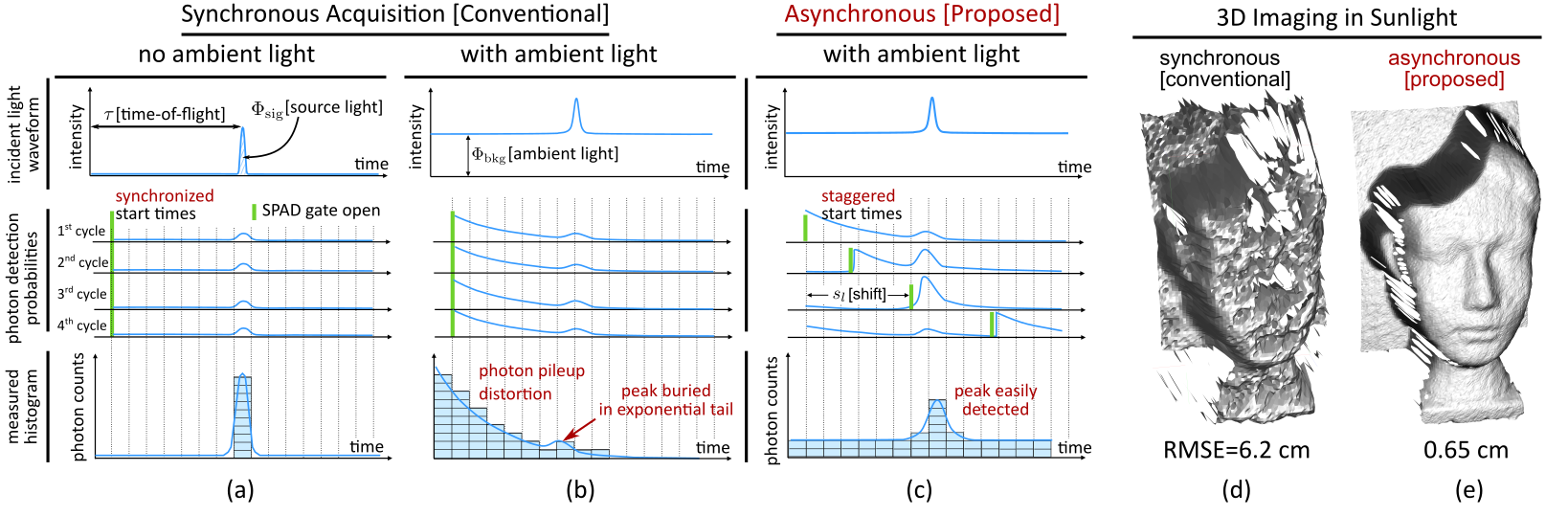
Figure 2: Imaging model of single-photon 3D cameras. (a) A single-photon 3D camera records the timestamps of returning photons over many laser cycles and constructs a histogram of photon arrival times. In the absence of ambient light, the peak of this histogram corresponds to the true depth. (b) In the conventional (synchronous) operation, ambient light causes photon pileup which distorts the histogram towards earlier time bins. (c) Asynchronous acquisition prevents pileup by temporally staggering the SPAD cycles with respect to the laser cycles, distributing the effect of pileup uniformly over all histogram bins. (d) 3D shape recovered using synchronous acquisition shows large depth errors due to pileup. (e) Proposed asynchronous method recovers accurate 3D shape even in high ambient light.

Light is fundamentally quantized; any camera records incoming light not continuously, but in discrete packets called photons. A conventional camera typically captures hundreds to thousands of photons per pixel to create an image. What if cameras could record individual photons, and, precisely measure their time-of-arrival? Not only would such cameras have extremely high sensitivity, but the captured data will have an additional time-dimension, a rich source of information inaccessible to conventional cameras.

There is an emerging class of sensors, called single-photon avalanche diodes (SPADs) [30] that promise single-photon sensitivity (Fig. 1(a)) and the ability to time-tag photons with picosecond precision. Due to these capabilities, SPADs are driving novel functionalities such as non-line-of-sight (NLOS) imaging [7, 22] and microscopy of bio-phenomena at nano time-scales [4]. However, so far, SPADs are considered specialized devices suitable only for photon-starved (dark) scenarios, and thus, restricted to a limited set of niche applications. This raises the following questions: Can SPADs operate not just in low-light, but across the entire gamut of imaging conditions, including high-flux scenes [15]? In general, is it possible to leverage the exciting capabilities of SPADs for a broader set of mainstream computer vision applications (Fig. 1(b))?

In this paper, we address the above questions in the context of 3D imaging. Consider a single-photon 3D camera based on time-of-flight (ToF). It consists of a pulsed laser emitting periodic pulses of light toward the scene, and a SPAD sensor (Fig. 1(c)). Although several conventional 3D cameras also use the ToF principle, single-photon 3D cameras have a fundamentally different imaging model. The SPAD detects at most one returning photon per laser pulse, and records its time-of-arrival. Arrival times over several laser pulses are recorded to create a temporal histogram of photon arrivals, as shown in Fig. 2(a). Under low incident flux, the histogram is approximately a linearly scaled replica of the incident waveform, and thus, can be used to recover scene depths [27, 19]. Due to the high timing resolution of SPADs, single-photon 3D cameras are capable of achieving “laser-scan quality” depth resolution (1–10 mm), at long distances (100–1000 meters) (Fig. 1(d)).

Single-photon 3D imaging in sunlight: Due to the peculiar histogram formation process, single-photon 3D cameras cannot operate reliably under ambient light (e.g., sunlight in outdoor conditions). This is because early arriving ambient photons prevent the SPAD from measuring the signal (laser) photons that may arrive at a later time bin of the histogram. This distorts the histogram measurements towards earlier time bins, as shown in Fig. 2(b). This non-linear distortion, known as photon pileup [14, 25, 17] makes it challenging to reliably locate the laser pulse, resulting in large depth errors. Although there has been a lot of research toward correcting these distortions in post-processing [14, 9, 23, 25, 28], strong pileup due to ambient light continues to limit the scope of this otherwise exciting technology.

We propose asynchronous single-photon 3D imaging, a family of computational imaging techniques for SPAD-based 3D cameras with the goal of preventing pileup during acquisition itself. In conventional ToF cameras, the laser and sensor are temporally synchronized. In contrast, we desynchronize the SPAD acquisition windows with respect to the laser pulses. This introduces different temporal offsets between laser cycles and SPAD acquisition windows, as shown in Fig. 2(c). The key insight is that cycling through a range of temporal offsets (across different laser cycles) enables detecting photons in later time bins that would otherwise have been masked by early-arriving ambient photons. This distributes the effect of pileup across all histogram bins, thus eliminating the structured distortions caused by the synchronous measurements, as shown in Fig. 2(c).

At first glance, it may appear that such asynchronous measurements may not provide consistent depth information. The main idea lies in computationally re-synchronizing the photon timing measurements with the laser cycles. To this end, we develop a generalized image formation model and derive a maximum likelihood estimator (MLE) of the true depth that accounts for arbitrary temporal offsets between measurement and laser cycles. Based on these ideas, we propose two asynchronous acquisition methods: uniform and photon-driven, which shift the SPAD window with respect to laser either deterministically or stochastically. These techniques can be implemented with minimal modifications to existing systems, while achieving up to an order-of-magnitude improvements in depth accuracy. An example is shown in Fig. 2(d–e).

Implications and future outlook: Due to their compatibility with mainstream CMOS sensor fabrication lines, the capabilities of SPAD cameras continue to grow rapidly [11, 32, 12, 20, 18, 1, 3]. As a result, the proposed methods, aided by rapid ongoing advances in SPAD technology, will potentially spur wide-spread adoption of single-photon sensors as all-purpose cameras in demanding computer vision and robotics applications, where the ability to perform reliably in both photon-starved and photon-flooded scenarios is critical to success.

2 Related Work

Photon pileup mitigation for SPAD cameras: Perhaps the most widely adopted approach for preventing pileup is attenuation, i.e., optically blocking the total photon flux incident on the SPAD so that only 1-5% of the laser pulses lead to a photon detection [2, 3]. Recent work [14, 13] has shown that this rule-of-thumb extreme attenuation is too conservative and the optimal operating flux is considerably higher. Various computational [25, 14] and hardware [1, 3, 35] techniques for mitigating pileup have also been proposed. These approaches are complementary to the proposed asynchronous acquisition, and can provide further improvements in performance when used in combination.

Temporally shifted gated acquisition: Fast-gated detectors [6] have been used previously for range-gated LiDAR, confocal microscopy and non-line-of-sight (NLOS) imaging [7] to preselect a specific depth range and suppress undesirable early-arriving photons. A sequence of shifted SPAD gates has been used in FLIM for improving temporal resolution and dynamic range [34, 31, 32] and for extending the unambiguous depth range of pulsed LiDARs [29]. In contrast, we use shifting to mitigate pileup and present a theoretically optimal method for choosing the sequence of shifts and durations of the SPAD measurement gates without any prior knowledge of scene depths.

Photon-driven acquisition: The photon-driven (or free-running) mode of operation has been analyzed for FLIM [16, 9, 1], and recently for LiDAR [28] where a Markov chain model-based iterative optimization algorithm is proposed to recover the incident waveform from the distorted histogram. The focus of these approaches is on designing efficient waveform estimation algorithms. Our goal is different. We explore the space of asynchronous acquisition schemes with the aim of designing acquisition strategies that mitigate depth errors due to pileup in high ambient light under practical constraints such as a fixed time budget. We also propose a generalized closed-form maximum likelihood estimator (MLE) for asynchronous acquisition that can be computed without any iterative optimization routine.

3 Single-Photon 3D Imaging Model

A SPAD-based 3D camera consists of a pulsed laser that emits short periodic pulses of light toward a scene point, and a co-located SPAD sensor that captures the reflected photons (Fig. 1(c)). Although the incident photon flux is a continuously varying function of time, a SPAD has limited time resolution, resulting in a discrete sampling of the continuous waveform. Let $\Delta$ denote the size of each discrete temporal bin (usually on the order of few tens of picoseconds). Assuming an ideal laser pulse modeled as a Dirac-delta function $\delta(t)$, the number of photons incident on the SPAD in the $i^{\text{th}}$ time bin follows a Poisson distribution with a mean given by:

$$r_{i}=\Phi_{\text{sig}}\delta_{i,\tau}+\Phi_{\text{bkg}}\,,$$ (1)

where $\delta_{i,j}$ is the Kronecker delta, $\tau=\lfloor\nicefrac{{2z}}{{c\Delta}}\rfloor$ is the discretized round-trip time delay, $z$ is the distance of the scene point from the camera, and $c$ is the speed of light. $\Phi_{\text{sig}}$ is the mean number of signal photons (due to the laser pulse) received per bin, and $\Phi_{\text{bkg}}$ is the (undesirable) background and dark count photon flux per bin. $B$ is the number of time bins in a single laser period. The vector $\left(r_{i}\right)_{i=1}^{B}$ denotes the incident photon flux waveform. A reliable estimate of this waveform is needed to estimate scene depth.

Synchronous acquisition: In order to estimate the incident waveform, SPAD-based 3D cameras employ the principle of time-correlated single-photon counting (TCSPC) [21, 17, 2, 26, 24, 25]. In conventional synchronous acquisition, the SPAD starts acquiring photons immediately after the laser pulse is transmitted, as shown in Fig. 2(a). In each laser cycle (laser repetition period), after detecting the first incident photon, the SPAD enters a dead time (${\sim}$$100\text{\,}\mathrm{ns}$) during which it cannot detect additional photons. The SPAD may remain inactive for longer than the dead time so that the next SPAD acquisition window aligns with the next laser cycle. The time of arrival of the first incident photon is recorded with respect to the start of the most recent cycle. A histogram $(N_{1},\!\ldots,\!N_{B})$ of the first photon arrival times is constructed over many cycles, where $N_{i}$ denotes the number of times the first photon arrives in the $i^{\text{th}}$ bin. In low ambient light, the histogram, on average, is simply a scaled version of the incident waveform [13], from which, depth can be estimated by locating its peak.

Effect of ambient light in synchronous acquisition: Under ambient light, the incident flux waveform can be modeled as an impulse with a constant d.c. offset, as shown in the top of Fig. 2(b). In high ambient flux, the SPAD detects an ambient photon in the earlier histogram bins with high probability. This skews the measured histogram towards earlier histogram bins, as shown in the bottom of Fig. 2(b). The peak due to the laser source appears only as a small blip in the exponentially decaying tail of the measured histogram. This distortion, called photon pileup [8, 2, 25], significantly lowers the accuracy of depth estimates.

In the next two sections we introduce a generalization of the synchronous TCSPC acquisition scheme, and show how it can be used to mitigate pileup distortion and reliably estimate depths, even in the presence of high ambient light.

4 Theory of Asynchronous Image Formation

In this section we develop a theoretical model for asynchronous single-photon 3D cameras. We derive a histogram formation model and a generalized Coates’s estimator [8] for the incident photon flux waveform. In asynchronous acquisition, we decouple the SPAD on/off times from the laser cycles by allowing the SPAD acquisition windows to have arbitrary start times with respect to the laser pulses (Fig. 2(c)). A SPAD cycle is defined as the duration between two consecutive time instants when the SPAD sensor is turned on. The SPAD will remain inactive during some portion of each SPAD cycle due to its dead time.

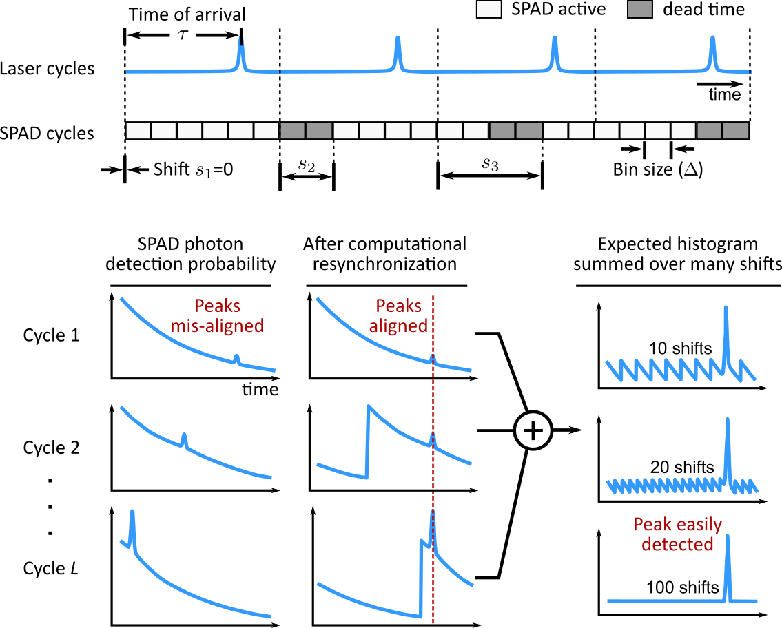
Figure 3: Histogram formation for asynchronous aquisition. (Top) The temporal location of the laser peak in the incident waveform corresponds to the round-trip time-of-flight. A slightly longer SPAD cycle period results in a sequence of increasing shifts with respect to the laser cycles. (Bottom) The histogram formation process involves computational resynchronization of photon arrival times to the laser cycle boundaries, causing a “wrap around.” The measured histogram approaches the true waveform shape when a large number of uniformly spaced shifts is used.

Each laser cycle consists of $B$ time bins which are used to build a photon count histogram. The bin indices are defined with respect to the start of the laser cycle, i.e., the first time bin is aligned with the transmission of each laser pulse. We assume that the laser repetition period is $B\Delta=2z_{\text{max}}/c$. This ensures that a photon detected by the SPAD always corresponds to an unambiguous depth range $[0,z_{\text{max}})$. Let $s_{l}$ ($0\leq s_{l}\leq B-1$) denote the bin index (with respect to the most recent laser cycle) at which the SPAD gate is activated during the $l^{\text{th}}$ SPAD cycle ($1\leq l\leq L$). As shown in Fig. 3(top), a SPAD cycle may extend over multiple consecutive laser cycles.

Probability distribution of measured histogram: Due to Poisson statistics, the probability $q_{i}$ that at least one photon is incident on the SPAD in the $i^{\text{th}}$ bin is:

$$q_{i}=1-e^{-r_{i}},$$ (2)

where $r_{i}$ is given by Eq. (1). A photon detection in the $i^{\text{th}}$ time bin occurs when no photon is incident in the time bins preceding the $i^{\text{th}}$ bin in the current cycle, and at least one photon is incident in the $i^{\text{th}}$ bin. The probability $p_{l,i}$ of a photon detection in the $i^{\text{th}}$ bin in the $l^{\text{th}}$ SPAD cycle depends on the shift $s_{l}$, and is given by:

$$p_{l,i}\hskip 3.61371pt =\hskip 3.61371ptq_{i}\hskip 3.61371pt\prod_{j:j<i}(1-q_{j})\,,$$ (3)

where it is understood (see Supplementary Note 1) that $j<i$ denotes the bin indexes preceding the $i^{\text{th}}$ bin in a modulo-B sense with a “wrap around” depending on the shift $s_{l}$ (Fig. 3(bottom)). We introduce an additional $(B\!+\!1)^{\text{th}}$ bin in the histogram to record the number of cycles where no photons were detected, with corresponding bin probability $p_{l,B+1}\!:=\!1\!-\!\sum_{i=1}^{B}p_{l,i}$.

As in the synchronous case, we construct a histogram of the number of photons detected in each time bin. Let $N_{i}$ be the number of photons captured in the $i^{\text{th}}$ bin over $L$ SPAD cycles. As shown in Supplementary Note 1, the joint distribution of the measured histogram $(N_{1},N_{2},\ldots,N_{B},N_{B+1})$ is given by a Poisson-Multinomial Distribution (PMD) [10]. The PMD is a generalization of the multinomial distribution; if $s_{l}=0\,\forall\,l$ (conventional synchronous operation), this reduces to a multinomial distribution [14, 25].

Characterizing pileup in asynchronous operation: Similar to the synchronous case, in the low incident flux regime ($r_{i}\ll 1\,\forall\,i$) the measured histogram is, on average, a linearly scaled version of the incident flux: $\mathbb{E}[N_{i}]\approx Lr_{i}$, and the incident flux can be estimated as $\widehat{r}_{i}=\nicefrac{{N_{i}}}{{L}}$. However, in high ambient light, the photon detection probability at a specific histogram bin depends on its position with respect to the beginning of the SPAD cycle. Similar to synchronous acquisition, histogram bins that are farther away from the start of the SPAD cycle record photons with exponentially smaller probabilities compared to those near the start of the cycle. However, unlike the synchronous case, the shape of this pileup distortion wraps around at the $B^{\text{th}}$ histogram bin during computational resynchronization. This is shown in Fig. 3(bottom). The segment that is wrapped around depends on $s_{l}$ and may vary with each SPAD cycle.

Computational pileup correction in asynchronous acquisition: A computational pileup correction algorithm must use the histogram $(N_{i})_{i=1}^{B+1}$ to estimate the true waveform $r_{i}$ via an estimate of $q_{i}$ and Eq. (2). Recall that a photon detection in a specific histogram bin prevents subsequent bins from recording a photon. Therefore, in the high flux regime, $q_{i}$ cannot be simply estimated as the ratio of $N_{i}$ to the number of SPAD cycles ($L$); the denominator in this ratio must account for the number of SPAD cycles where the $i^{\text{th}}$ histogram bin had an opportunity to record a photon.

Definition 1 (Denominator Sequence).

Let $D_{l,i}$ be an indicator random variable which is $1$ if, in the $l^{\text{th}}$ SPAD cycle, no photon was detected before the $i^{\text{th}}$ time bin. The denominator sequence $(D_{i})_{i=1}^{B}$ is defined as $D_{i}=\sum_{l=1}^{L}D_{l,i}$.

Note that $D_{l,i}=1$ indicates that in the $l^{\text{th}}$ SPAD cycle, the SPAD had an opportunity to detect a photon in the $i^{\text{th}}$ bin. By summing over all SPAD cycles, $D_{i}$ denotes the total number of photon detection opportunities in the $i^{\text{th}}$ histogram bin. Using this corrected denominator, an estimate for $q_{i}$ is obtained as follows:

$$\widehat{q}_{i}=\frac{N_{i}}{D_{i}}\,.$$

We show in Supplementary Note 1 that $\widehat{q}_{i}$ is in fact the MLE of $q_{i}$. The MLE of the incident flux waveform is given by:

$$\widehat{r}_{i}=\ln\left(\frac{1}{1-\widehat{q}_{i}}\right)$$ (4)

which is a generalization of the Coates’s estimator [8, 25]. Photon pileup causes later histogram bins to have $D_{i}\approx 0$ making it difficult to estimate $r_{i}$. Intuitively, a larger $D_{i}$ denotes more “information” in the $i^{\text{th}}$ bin, hence a more reliable estimate of the true flux waveform can be obtained.

5 Photon Pileup: Prevention Better than Cure?

In theory, when operating in high ambient light, the generalized Coates’s estimator in Eq. (4) can invert pileup distortion for asynchronous acquisition with any given set of shifts $s_{l}$. However, if the asynchronous acquisition scheme is not well-designed, this inversion will lead to unreliable waveform estimates. For example, if the shifts $s_{l}$ are all zero (synchronous acquisition), bins farther from the start of the SPAD cycle will have $D_{i}\approx 0$ and suffer from extremely noisy flux estimates.

In this section, we design imaging techniques that prevent photon pileup in the acquisition phase itself, even under high ambient light. Our main observation is that delaying the start of the SPAD cycle with respect to the start of a laser cycle increases $D_{i}$ at later time bins. The key idea, as shown in Fig. 3, is to cycle through various shifts $s_{l}$ for different SPAD cycles. This ensures that each time bin is close to the start in at least a few SPAD cycles. Intuitively, if all possible shifts from $0$ to $B\!-\!1$ are used, the effect of the exponentially decaying pileup due to ambient photons gets distributed over all histogram bins equally. On the other hand, returning signal photons from the true laser peak add up “coherently” because their bin location remains fixed. As a result, the accumulated histogram has enough photons in all bins (Fig. 3(e)) to enable reliable Coates’s estimates.

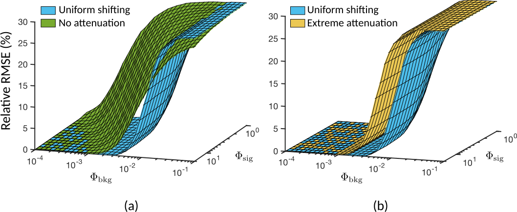
Figure 4: Simulated depth RMSE at different ambient and signal flux levels. Asynchronous acquisition with uniform shifting achieves lower error than synchronous acquisition with no and extreme attenuation [13], over a wide range of flux conditions.

We characterize the space of all shifting strategies by their shift sequence, $(s_{i})_{i=1}^{L}$. For now, we only consider deterministic shift sequences, which means that the shifts are fixed and known prior to acquisition. Given these definitions, the question that we seek to address is: What is the optimal shifting strategy that minimizes depth estimation error? We now present two key theoretical results towards answering this question for a SPAD-based 3D camera operating in the high ambient flux regime where the total number of incident photons is dominated by ambient photons.

Definition 2 (Uniform Shifting).

A shifting strategy is said to be uniform if its shift sequence is a uniform partition of the time interval $[0,B\Delta)$, i.e., is a permutation of the sequence $\left(0,\lfloor\nicefrac{{B}}{{L}}\rfloor,\lfloor\nicefrac{{2B}}{{L}}\rfloor,...,\lfloor\nicefrac{{(L-1)B}}{{L}}\rfloor\right)$.

Result 1 (Denominator Sequence and Probability of Depth Error).

In the high ambient flux regime, among all denominator sequences with a fixed total expected sum $\sum_{i=1}^{L}\mathbb{E}[D_{i}]$, an upper bound on the average probability of depth error for the estimator in Eq. (4) is minimized when $\mathbb{E}[D_{i}]=\mathbb{E}[D_{j}]\,\forall\,i,j$.

Result 2 (Denominator Sequence for Uniform Shifting).

Uniform shifting achieves a constant expected denominator sequence.

Interpreting Results 1 and 2: As shown in Supplementary Note 2, for a fixed $L$, different shift sequences will lead to different denominator sequences but the total expected denominator $\sum_{i=1}^{L}\mathbb{E}[D_{i}]$ remains constant. The first result (based on [13]) shows that if a shifting strategy can achieve a constant expected denominator sequence, it will have lower depth error than all other shifting strategies (including synchronous acquisition). The second result shows that there exists a shifting strategy that achieves a constant expected denominator: uniform shifting. As a byproduct, a uniform denominator sequence makes the depth errors invariant to the true bin location, unlike the synchronous case where later time bins suffer from higher depth errors.

Single-pixel simulations: We compare the performance of uniform shifting and conventional synchronous acquisition through Monte Carlo simulations. We use a histogram with $B=1000$ and $\Delta=$100\text{\,}\mathrm{ps}$$ and consider a wide range of background and signal photon flux levels in the discrete delta pulse model of Eq. (1). Uniform shifts are simulated by choosing equally spaced shifts between $0$ and $1000$ and generating photon counts using Eq. (S3). Depth is estimated using the generalized estimator (Eq. (4)). As seen in Fig. 4, the depth RMSE with uniform shifting is considerably lower than conventional synchronous acquisition. At certain combinations of signal and background flux levels, uniform shifting estimates depths with almost zero RMSE while the conventional methods give a very high error.

6 Practically Optimal Acquisition for Single-Photon 3D Imaging in Bright Sunlight

The theoretical analysis in the previous section shows uniform shifting minimizes an upper bound on the $\ell_{0}$ depth error. It is natural to ask: How can we implement practical uniform shifting approaches that are not just theoretically optimal in the $\ell_{0}$ sense, but also achieve good RMSE ($\ell_{2}$ error) performance under realistic constraints and limited acquisition time? In this section, we design several high-performance shifting schemes based on uniform shifting. These are summarized in Fig. 5.

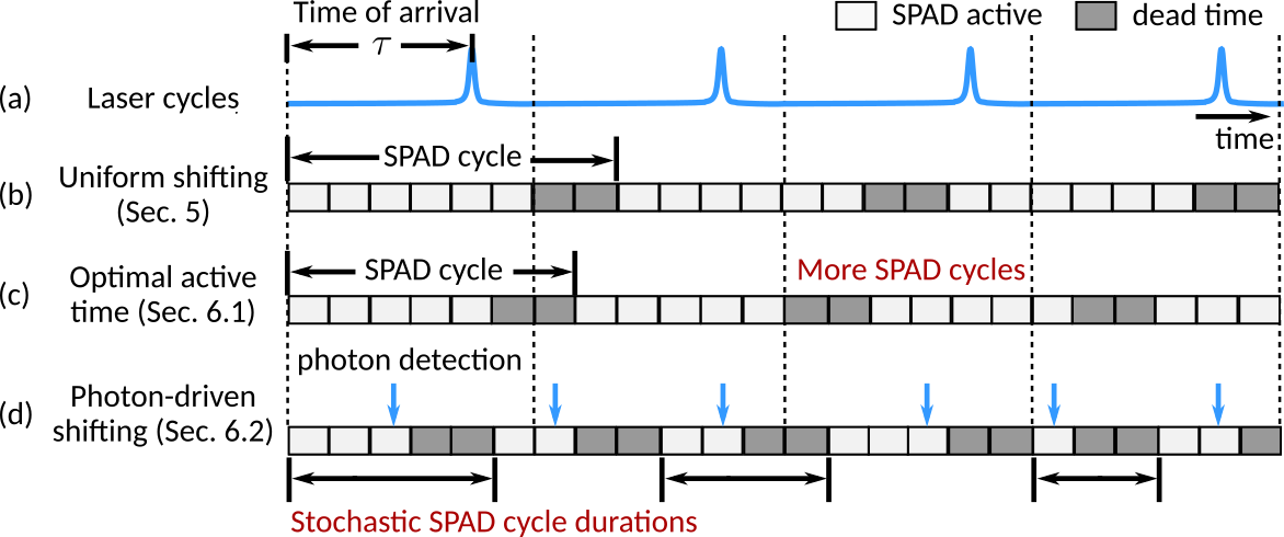
Figure 5: Different asynchronous acquisition methods. (a) The incident waveform has a period equal to the laser cycle period. (b) Uniform shifting staggers the laser and SPAD cycles by introducing a mismatch in cycle lengths. (c) Optimizing the SPAD active time enables more SPAD cycles to fit within a fixed total capture time. (d) Photon-driven shifting has random SPAD cycle lengths determined by photon detection events.

Uniform shifting can be implemented in practice by making the SPAD cycle period longer than the laser cycle (Fig. 5(b)), and relying on this mismatch to automatically cycle through all possible shifts. Moreover, this can be implemented at a negligible additional cost in terms of total acquisition time as shown in Supplementary Note 3.

6.1 SPAD Active Time Optimization

So far, we have assumed the SPAD active time duration is fixed and equal to $B\Delta$. Programmable fast-gated SPAD detectors [6, 5] allow flexibility in choosing different active time and SPAD cycle durations (Fig. 5(c)). Arbitrary shift sequences can also be implemented by varying the number of active time bins, $m$, while keeping the inactive duration fixed at $t_{\text{d}}$. This expands the space of shifting strategies characterized by the active time bins, $m$, and the shift sequence, $(s_{l})_{l=1}^{L}$. Under a fixed acquisition time constraint:

$$L(m\Delta+t_{d})\leq T.$$ (5)

Note that $L$ can now vary with $m$. Can this greater design flexibility be used to improve depth estimates?

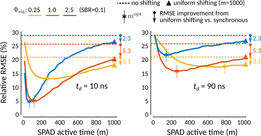
Figure 6: Effect of SPAD active time on performance. This plot shows the improvement in RMSE from SPAD active time optimization at different signal strengths and dead times. Note that the RMSE gain (size of vertical arrows) due to uniform shifting over synchronous acquisition remains unchanged across dead times. For low flux levels and long dead times, a longer active time improves RMSE by enabling the SPAD to capture more photons.

Varying $m$ leads to an interesting trade-off. Shortening the active time duration causes a larger proportion of each SPAD cycle to be taken up by dead time. On the other hand, using a very long active time is inefficient because the portion of the active time after the first photon arrival is spent in dead time anyway. This raises the question: What is the optimal active time that minimizes the depth error? In Supplementary Note 4 we show that the optimal active time for uniform shifting is given by:

$$m^{\text{opt}}=\operatorname*{arg\,max}_{m}\frac{T}{m\Delta+t_{\text{d}}}\frac{1-e^{-m\Phi_{\text{bkg}}}}{1-e^{-\Phi_{\text{bkg}}}}.$$ (6)

Simulation results for varying active time: Fig. 6 shows plots of depth RMSE vs. $m$ for a wide range of ambient flux levels and two different values of dead time. Observe that the RMSE curves have local minima which agree with our theory (Eq. (6)). For a wide range of photon flux levels considered here, $m^{\text{opt}}$ is shorter than the conventionally used active time of $m=B=1000$ and gives a remarkable improvement in RMSE by up to a factor of $6$.

6.2 Photon-Driven Shifting

The optimal active time criterion balances the tradeoff between short and long active time windows in an average sense. However, due to the large variance in the arrival time of the first photon in each cycle, a fixed $m$ cannot achieve both these goals on a per-photon basis. It is possible to achieve photon-adaptive active time durations using the free-running mode [28] where the SPAD is always active, except after a photon detection when it enters a dead time.

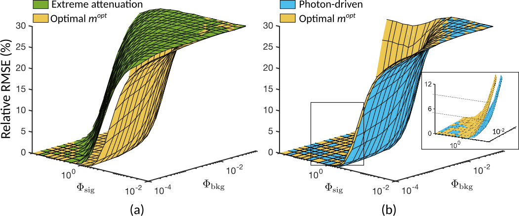
Figure 7: Simulation-based evaluation of practically optimal asynchronous acquisition. (a) Asynchronous acquisition with optimal SPAD active time (Section 6.1) provides an order of magnitude lower depth RMSE as compared to existing methods. (b) Photon-driven shifting (Section 6.2) further lowers RMSE by allowing the active time to vary stochastically on a per-photon basis.

In the free-running mode the active times and SPAD cycle durations vary randomly due to the stochastic nature of photon arrivals. As shown in Fig. 5(d), this creates different shifts across different SPAD cycles. Over a sufficiently long acquisition time, a uniformly spaced sequence of shifts is achieved with high probability, distributing the effect of pileup over all histogram bins uniformly. We call this randomized shifting phenomenon photon-driven shifting.

Depth estimator for photon-driven shifting: Unlike deterministic shifting, the shift sequence in photon-driven shifting is stochastic because it depends on the random photon arrival times. In Supplementary Note 5 we show that the scene depths can still be estimated using the generalized Coates’s estimator (Eq. (4)) as before.

The following result states that photon-driving shifting possesses the desirable property of providing a uniform shift sequence. See Supplementary Note 5 for a proof.

Result 3.

As $L\rightarrow\infty$, photon-driven shifting achieves a uniform shift sequence.

Result 3 says that photon-driven shifting exhibits a pileup averaging effect, similar to uniform shifting. Although this does not establish a relationship between the shift sequence and depth RMSE, our results show up to an order of magnitude improvement in RMSE compared to conventional synchronous acquisition.

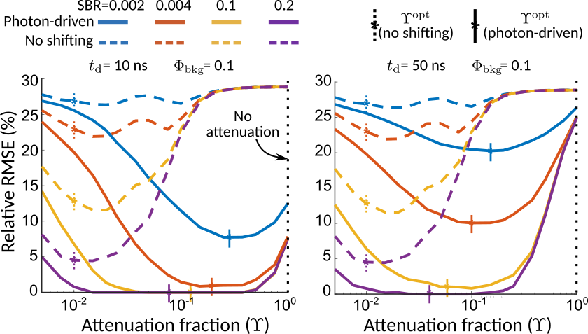
Figure 8: Optimal attenuation factor $\Upsilon^{\text{opt}}$ for photon-driven shifting is higher than that of synchronous acquisition, leading to efficient flux utilization, while minimizing photon pileup.

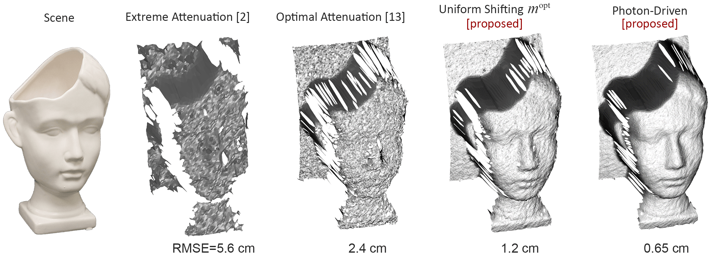
Figure 9: Experimental demonstration of single-photon 3D imaging under strong ambient light. A white “PorcelainFace” vase was illuminated with high ambient light of $B\Phi_{\text{bkg}}=11$ photons and scanned with a low-power laser at an SBR of $0.02$. The proposed asynchronous acquisition schemes achieve considerably higher depth quality as compared to conventional synchronous methods.

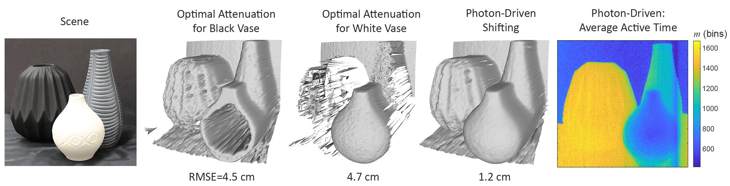
Figure 10: Adaptivity of photon-driven shifting to different albedos. The black vase in this “Vases” scene has $\nicefrac{{1}}{{10}}^{\text{th}}$ the reflectivity of the white vase. With synchronous acquisition, the attenuation fraction must be adjusted individually for each vase. In contrast, both vases are reliably reconstructed with photon-driven shifting which automatically adapts the active time duration for each pixel.

Simulation results: Fig. 7 shows simulated RMSE results for photon-driven shifting over a wide range of signal and ambient flux levels. For some flux levels the proposed shifting methods provide almost zero depth error while the conventional method has the maximum possible error. The RMSE of photon-driven shifting is similar to uniform shifting with $m^{\text{opt}}$, but for some flux levels it can provide a factor of $2$ improvement over uniform shifting. Supplementary Note 6 discusses certain regimes where deterministic shifting may be preferable over photon-driven shifting.

6.3 Combination with Flux Attenuation

Recent work [13, 14] has shown that there is an optimal incident flux level at which pileup in a synchronous SPAD-based 3D camera is minimized while maintaining high SNR. This optimal flux can be achieved by optically attenuating the incident photon flux. In the space of acquisition strategies to deal with pileup, attenuation can be considered a complementary approach to asynchronous shifting. In Supplementary Note 7, we show that the optimal attenuation fraction for photon-driven shifting is given by:

$$\Upsilon^{\text{opt}}_{\text{photon-driven}}=\min\left\{1.0,\operatorname*{arg\,min}_{\Upsilon}\frac{1+t_{\text{d}}(1-e^{-\Upsilon\Phi_{\text{bkg}}})}{e^{-\Upsilon\Phi_{\text{bkg}}}(1-e^{-\Upsilon\Phi_{\text{sig}}})}\right\}.$$

Fig. 8 shows simulation results of depth RMSE for the conventional synchronous mode and photon-driven shifting over a range of attenuation factors and two different dead times. The locations of the minima agree with our theory. There are two key observations. First, the optimal attenuation fraction with shifting is much higher than that for conventional synchronous acquisition. Second, combining attenuation with photon-driven shifting can provide a large gain in depth error performance, reducing the RMSE to almost zero under certain conditions.

7 Experiments

Our hardware prototype consists of a $405\text{\,}\mathrm{nm}$ pulsed laser (Picoquant LDH-P-C-405B), a TCSPC module (Picoquant HydraHarp 400) and a fast-gated SPAD [6] that can be operated in both triggered and free-running modes and has a programmable dead time which was set to $50\text{\,}\mathrm{ns}$. We operated the laser at a repetition frequency of $10\text{\,}\mathrm{MHz}$ for an unambiguous depth range of $15\text{\,}\mathrm{m}$ discretized into $1000$ histogram bins. For uniform shifting, we operated the SPAD with its internal clock to obtain shifts between the SPAD measurement windows and the laser cycles.

3D point-scanning results: Fig. 9 shows 3D reconstructions of “PorcelainFace” scene under high ambient illumination. Both uniform and photon-driven shifting ($\Upsilon^{\text{opt}}_{\text{photon-driven}}=1$) perform better than synchronous acquisition methods. Photon-driven acquisition provides sub-centimeter RMSE, which is an order of magnitude better than the state-of-the-art extreme attenuation method.

The method of [13] uses synchronous acquisition and relies on setting an attenuation factor for different parts of the scene based on the total photon flux and hence requires pixel-wise adaptation. The “Vases” scene in Fig. 10 consists of a black vase with a much lower albedo than the white vase. The attenuation fraction needed for the white vase is too low and causes the black vase to appear noisy, whereas the attenuation fraction for the black vase is too high to avoid pileup distortions at the white vase. The average active time with photon-driven shifting ($\Upsilon^{\text{opt}}_{\text{photon-driven}}=1$) automatically adapts to different photon flux levels and reliably captures the depth map for both vases. For darker scene points the average active time is longer than the laser cycle period of $B=1000$.

8 Limitations and Discussion

Incorporating spatial priors: The theoretical analysis and results presented here are limited to a pixel-wise depth estimator which uses the MLE of the photon flux waveform. Further improvements can be obtained by incorporating spatial priors in a regularized optimization framework [14], or data-driven neural network-based approaches [19] that exploit spatial correlations between neighboring pixels and across different training images to improve depth accuracy.

Extension to other active-imaging modalities: The idea of using asynchronous acquisition schemes can be extended to other SPAD-based active-imaging applications that use the principle of TCSPC to recover the true shape of the photon flux waveform. Non-uniform shifting schemes may be required for time-domain FLIM where true waveform shape is an exponential decay and NLOS imaging where the photon flux waveform can have arbitrary shapes.

Supplementary Note 1 Asynchronous Image Formation Model and MLE Waveform Estimator

In this supplementary note we derive the Poisson-Multinomial histogram model of Eq. (S3) in the main paper. We then derive the generalized Coates’s estimator (Eq. (4)), which is the maximum likelihood estimator (MLE) of the photon flux waveform in asynchronous acquisition. Scene depth is computed by locating the peak of the estimated photon flux waveform.

Joint Distribution of Measured Histogram

Here we derive the joint distribution of the histogram $(N_{1},\ldots,N_{B},N_{B+1})$ measured in the asynchronous acquisition mode. Recall that the $B+1^{\text{st}}$ bin is added for mathematical convenience to record SPAD cycles with no detected photons. For the $l^{\text{th}}$ SPAD cycle we define a one-hot random vector $(O_{l,1},O_{l,2},\ldots,O_{l,B},O_{l,B+1})$ that stores the bin index where the photon was recorded. Since the SPAD detects at most one photon per laser cycle, $(O_{l,i})_{i=1}^{B+1}$ contains zeroes everywhere except at the bin index corresponding to the photon detection. Its joint distribution is given by a categorical distribution [Suppl. Ref. 1]:

$$(O_{l,i})_{i=1}^{B+1}\sim\text{($B\!+\!1$)-Categorical}\big{(}(p_{l,i})_{i=1}^{B+1}\big{)}.$$ (S1)

The final histogram of photon counts is obtained by summing these one-hot vectors over all laser cycles:

$$N_{i}=\sum_{l=1}^{L}O_{l,i}\,.$$ (S2)

Since $N_{i}$ is a sum of $L$ different ($B\!+\!1$)-Categorical random variables, the joint distribution is given by a Poisson-Multinomial Distribution [Suppl. Ref. 2]:

$$(N_{i})_{i=1}^{B+1}\sim\text{$(L,B\!+\!1)$-PMD}\bigg{(}(p_{l,i})_{1\leq l\leq L,1\leq i\leq B+1}\bigg{)}.$$ (S3)

The expected number of photon counts $\mathbb{E}[N_{i}]$ in the $i^{\text{th}}$ bin is $\sum_{l=1}^{L}p_{l,i}$. Note that in the synchronous case, this reduces to a multinomial distribution because the one-hot random vector defined here no longer depends on the SPAD cycle index $l$.

Derivation of the Generalized Coates’s Estimator for Asynchronous SPAD LiDAR (Eq. (4))

In this section, we derive the MLE $(\widehat{r}_{i})_{i=1}^{B}$ of the true waveform $(r_{i})_{i=1}^{B}$ for the asynchronous acquisition model and show that it is equal to the generalized Coates’s estimator described in the main text. We assume that for each SPAD cycle $1\leq l\leq L$, the TCSPC system stores one-hot random vectors $(O_{l,i})_{1\leq i\leq B+1}$.

For future reference, we define $J_{l,i}$ to be the set of bin indices preceding $i$ in the $l^{\text{th}}$ cycle, in a modulo-B sense:

$$J_{l,i}\!=\!\begin{cases}\{s_{l}\!+\!1,\ldots,\!\underbrace{B,1}_{\text{wrap around}},\!\ldots,i\!-\!1\},&\text{for }i\leq s_{l}\\ \{s_{l}\!+\!1,\ldots,i\!-\!1\},&\text{for }i>s_{l}\,.\end{cases}$$ (S4)

In the $l\text{th}$ laser cycle, the joint distribution of $(O_{l,i})_{i=1}^{B+1}$ is given by the categorical distribution in Eq. (S1). Therefore, the likelihood function of the photon incidence probabilities $(q_{i})_{i=1}^{B}$ is given by:

$$\mathcal{L}(q_{1},q_{2},...,q_{B}) =\mathbb{P}\left((O_{1,i})_{i=1}^{B+1},(O_{2,i})_{i=1}^{B+1},...,(O_{L,i})_{i=1}^{B+1}|q_{1},q_{2},...,q_{B}\right)$$

$$\overset{(a)}{=}\prod_{l=1}^{L}\mathbb{P}\left((O_{l,i})_{i=1}^{B+1}|q_{1},q_{2},...,q_{B}\right)$$

$$\overset{(b)}{=}\prod_{l=1}^{L}\prod_{i=1}^{B+1}p_{l,i}^{O_{l,i}}$$

$$\overset{(c)}{=}\prod_{l=1}^{L}\prod_{i=1}^{B+1}{\left(q_{i}\prod_{j\in J_{l,i}}(1-q_{j})\right)}^{O_{l,i}}$$

$$\overset{(d)}{=}\prod_{i=1}^{B+1}q_{i}^{\sum_{l=1}^{L}O_{l,i}}\left[\prod_{l=1}^{L}\prod_{i=1}^{B+1}\left(\prod_{j=1}^{B+1}(1-q_{j})^{\mathbbm{1}(j\in J_{l,i})}\right)^{O_{l,i}}\right]$$

$$\overset{(e)}{=}\prod_{i=1}^{B+1}q_{i}^{N_{i}}\prod_{j=1}^{B+1}\prod_{l=1}^{L}(1-q_{j})^{\sum_{i=1}^{B+1}\mathbbm{1}(j\in J_{l,i}){O_{l,i}}}$$

$$\overset{(f)}{=}\prod_{i=1}^{B+1}q_{i}^{N_{i}}\prod_{j=1}^{B+1}\prod_{l=1}^{L}(1-q_{j})^{D_{l,j}-O_{l,j}}$$

$$\overset{(g)}{=}\prod_{i=1}^{B+1}q_{i}^{N_{i}}(1-q_{i})^{D_{i}-N_{i}}$$ (S5)

where (a) holds because measurements in different cycles are conditionally independent given the shift sequence; (b) follows from the definition of categorical distribution and the fact that for any fixed $l$, $O_{l,i}=1$ for exactly one $1\leq i\leq B+1$; (c) follows from Eq. (3); (d) uses the notation $\mathbbm{1}$ for the indicator function; (e) uses the definition of $N_{i}$ from Eq. (S2); (f) follows from the lemma proved below; (g) follows from Eq. (S2) and Def. 1 and rearrangement of the terms in the preceding product.

Since the likelihood is factorizable in $q_{i}$, we can calculate the MLE element-wise as:

$$\widehat{q}_{i} =\operatorname*{arg\,max}_{q_{i}}\;q_{i}^{N_{i}}(1-q_{i})^{D_{i}-N_{i}}$$

$$=\frac{N_{i}}{D_{i}}.$$

Since $q_{i}=1-e^{-r_{i}}$, by the functional invariance property of the MLE [Suppl. Ref. 4], the MLE for the photon flux waveform $r_{i}$ is given by the generalized Coates’s estimator of Eq. (4). We estimate scene depth by locating the peak of the estimated waveform: $\widehat{\tau}=\operatorname*{arg\,max}_{i}\widehat{r}_{i}.$

Finally, we prove the following lemma that was used in step (f) in the derivation above.

Lemma (Proof of step (f)).

For $1\leq j\leq B+1$ and $1\leq l\leq L$

$$\sum_{i=1}^{B+1}\mathbbm{1}(j\in J_{l,i}){O_{l,i}}=D_{l,j}-O_{l,j}$$

Proof.

Let $i^{*}$ denote the bin index where the photon was detected in the $l^{\text{th}}$ SPAD cycle, i.e., $O_{l,k}=1$ iff $k=i^{*}$ and $0$ otherwise. Then:

$$\sum_{i=1}^{B+1}\mathbbm{1}(j\in J_{l,i}){O_{l,i}}=\mathbbm{1}(j\in J_{l,i^{*}}){O_{l,i^{*}}}.$$

If $j=i^{*}$, then by definition $j\not\in J_{l,i^{*}}$. Therefore, LHS = 0. Also, $D_{l,j}=O_{l,j}=1$ in this case, so RHS = 0. If $j\neq i^{*}$, there are two cases. Case 1: $j\in J_{l,i^{*}}$. Then $D_{l,j}=1$ and $O_{l,j}=0$. Therefore, LHS = RHS = 1. Case 2: $j\not\in J_{l,i^{*}}$. Then $D_{l,j}=O_{l,j}=0$. Therefore, LHS = RHS = 0. ∎

Supplementary Note 2 Proofs of Results 1 and 2

In this section we provide detailed mathematical proofs for two key theoretical results in the main paper. Recall that we use an upper bound on the probability of depth error ($\ell_{0}$ error) as a surrogate for RMSE. Result 1 establishes the importance of a constant expected denominator sequence. It shows that a shifting strategy that minimizes an upper bound on the $\ell_{0}$ error must have a denominator sequence that is constant (on average) for all histogram bins. Result 2 shows that the uniform shifting strategy (which allocates approximately equal number of shifts to all histogram bins over whole depth range) achieves a constant expected denominator sequence.

Proof of Result 1

In this section, we will derive an upper bound on $\ell_{0}$ depth error which corresponds to the probability that the depth estimate using the generalized Coates’s estimator derived in Supplementary Note 1 is different from the true depth bin.

An upper bound on $\ell_{0}$ error:

To ensure that the depth estimate $\widehat{\tau}$ is correct, the bin corresponding to the true depth should have the highest counts after the generalized Coates’s correction (Eq. (4)) is applied. Therefore, for a given true depth $\tau$, we want to minimize the probability of depth error:

$$\mathbb{P}(\widehat{\tau}\neq\tau) =\mathbb{P}\left(\bigcup_{i\neq\tau}(\widehat{q}_{i}>\widehat{q}_{\tau})\right)$$

$$\leq\sum_{i\neq\tau}\mathbb{P}\left(\widehat{q}_{i}>\widehat{q}_{\tau}\right)$$

$$=\sum_{i\neq\tau}\mathbb{P}\left(\widehat{q}_{i}-\widehat{q}_{\tau}>0\right)$$

where the first inequality follows from the union bound. Note that $\widehat{q}_{i}-\widehat{q}_{\tau}$ has a mean $q_{i}-q_{\tau}$ and variance $\sigma^{2}_{i}+\sigma^{2}_{\tau}$ (assuming uncorrelated). The variance is given by [Suppl. Ref. 3] $\sigma_{i}^{2}=\frac{q_{i}(1-q_{i})}{\mathbb{E}[D_{i}]}.$

For large $L$, by the central limit theorem, we have:

$$\widehat{q}_{i}-\widehat{q}_{\tau}\sim\mathcal{N}(q_{i}-q_{\tau},\sigma^{2}_{i}+\sigma^{2}_{\tau}).$$

Using the Chernoff bound for Gaussian random variables, we get:

$$\mathbb{P}(\widehat{q}_{i}>\widehat{q}_{\tau}) \leq\exp{\left(-\frac{(q_{i}-q_{\tau})^{2}}{2(\sigma^{2}_{i}+\sigma^{2}_{\tau})}\right)}$$

$$=\frac{1}{2}\exp{\left(-\frac{1}{2}\frac{(q_{i}-q_{\tau})^{2}}{\frac{q_{i}(1-q_{i})}{\mathbb{E}[D_{i}]}+\frac{q_{\tau}(1-q_{\tau})}{\mathbb{E}[D_{\tau}]}}\right)}$$

Assuming a uniform prior on $\tau$ over the entire depth range, we get the following upper bound on the average probability of error:

$$\frac{1}{B}\sum_{\tau=1}^{B}\mathbb{P}(\widehat{\tau}\neq\tau) \leq\frac{1}{B}\sum_{\tau=1}^{B}\sum_{i\neq\tau}\frac{1}{2}\exp{\left(-\frac{1}{2}\frac{(q_{i}-q_{\tau})^{2}}{\frac{q_{i}(1-q_{i})}{\mathbb{E}[D_{i}]}+\frac{q_{\tau}(1-q_{\tau})}{\mathbb{E}[D_{\tau}]}}\right)}$$

$$\approx\frac{1}{B}\sum_{i,\tau=1}^{B}\frac{1}{2}\exp{\left(-\frac{1}{2}\frac{(q_{i}-q_{\tau})^{2}}{\frac{q_{i}(1-q_{i})}{\mathbb{E}[D_{i}]}+\frac{q_{\tau}(1-q_{\tau})}{\mathbb{E}[D_{\tau}]}}\right)}$$ (S6)

We can minimize the probability of error indirectly by minimizing this upper bound. The upper bound involves exponential quantities which will be dominated by the least negative exponent, which in turn is dominated by the index $i$ with the largest value of $\nicefrac{{1}}{{\mathbb{E}[D_{i}]}}.$ Therefore, the denominator sequence that minimizes this upper bound must maximize $\min_{i}\mathbb{E}[D_{i}]$. Given that the total expected denominator is constant under a fixed number of cycles (see proof below), this is equivalent to making the denominator sequence uniform.

The above analysis assumes that photon detections across cycles are independent, and therefore holds for all acquisition schemes with a gating mechanism that is fixed in advance, including synchronous and asynchronous acquisition (deterministic). Note that it does not hold for photon-driven shifting, where a photon detection in one cycle can affect that in another.

Proof of constant total expected denominator:

Let $\Xi\equiv\sum_{i=1}^{B}\mathbb{E}[D_{i}]$ be the total expected denominator. Assuming a low SBR scenario where the background flux dominates the signal flux, we take $r_{i}\approx\Phi_{\text{bkg}}$ for all $i$, i.e., an almost uniform incident waveform. To calculate the total denominator, we sum up the contributions of each cycle. If the SPAD active time is $m$, each cycle ends with either a photon detection in one of the $m$ time bins, or with no photon detections. A cycle with a photon detection in the $i^{\text{th}}$ bin ($1\leq i\leq m$) contributes $i$ units to the total denominator, since each bin before and including the detection bin was active. By the same argument, a cycle with no photon detections contributes $m$ units. Therefore, the total expected denominator is given by:

$$\Xi =\sum_{l=1}^{L}\left[\sum_{i=1}^{m}\mathbb{P}(O_{l,s_{l}\oplus i}=1)\cdot i+\mathbb{P}(O_{l,s_{l}\oplus i}=0\text{ for }1\leq i\leq m)\cdot m\right]$$

$$=\sum_{l=1}^{L}\left[\sum_{i=1}^{m}p_{l,s_{l}\oplus i}\cdot i+\left(1-\sum_{j=1}^{m}p_{l,s_{l}\oplus j}\right)\cdot m\right]$$

$$\overset{(a)}{=}\sum_{l=1}^{L}\left[\sum_{i=1}^{m}(1-e^{-\Phi_{\text{bkg}}})e^{-(i-1)\Phi_{\text{bkg}}}\cdot i+e^{-m\Phi_{\text{bkg}}}\cdot m\right]$$

$$=\frac{L(1-e^{-m\Phi_{\text{bkg}}})}{1-e^{-\Phi_{\text{bkg}}}}\;,$$ (S7)

where $\oplus$ denotes addition modulo-B, and (a) follows from the fact that for a uniform waveform, $p_{l,s_{l}\oplus i}=(1-e^{-\Phi_{\text{bkg}}})(e^{-\Phi_{\text{bkg}}})^{|J_{l,s_{l}\oplus i}|}$. Moreover, $J_{l,s_{l}\oplus i}=i-1$. Therefore, $\Xi$ remains constant for a given $L$, regardless of the shift sequence used.

Proof of Result 2

For $1\leq i\leq B$, under uniform shifting:

$$\mathbb{E}[D_{i}] \overset{(a)}{=}\sum_{l=1}^{L}\mathbb{E}[D_{l,i}]$$

$$=\sum_{l=1}^{L}\prod_{j\in J_{l,i}}(1-q_{j})$$

$$\overset{(b)}{\approx}\sum_{l=1}^{L}\prod_{j\in J_{l,i}}e^{-\Phi_{\text{bkg}}}$$

$$=\sum_{l=1}^{L}e^{-\Phi_{\text{bkg}}|J_{l,i}|}$$

$$=\sum_{l=1}^{L}e^{-\Phi_{\text{bkg}}\{(i-s_{l})\bmod B\}}$$

$$\overset{(c)}{=}\frac{L}{B}\left(\sum_{i=0}^{B-1}e^{-i\Phi_{\text{bkg}}}\right)$$

where (a) follows from Def. 1; (b) relies on the assumption that the pileup is mainly due to ambient light $\Phi_{\text{bkg}}$ and not the source light $\Phi_{\text{sig}}$; and (c) assumes that $L$ is a multiple of $B$. The last step follows because under uniform shifting, the set of shifts $\{s_{l}\}_{l=1}^{L}$ spans the discrete space $\{0,1,...,B-1\}$ uniformly. Moreover, the shifts remain uniform when transformed by a constant modulo addition. Therefore, $\mathbb{E}[D_{i}]$ is the sum of identical terms, and hence same for all $i$.

If $L$ is not a multiple of $B$, the shift sequence cannot achieve every possible shift from $0$ to $B-1$ an equal number of times and some bins might use more shifts than others, especially when $L<B$.However, the expected denominator sequence is still approximately uniform, with the approximation becoming more accurate as $L$ increases. This can be intuitively seen from the gradual elimination of the “saw teeth” in Fig. 3 as the number of shifts increases.

Supplementary Note 3 Achieving Uniform Shifts through Laser and SPAD Cycle Mismatch

The implementation shown in Fig. 3 relies on the SPAD cycle period being different from the laser cycle. By default, the duration for which the SPAD gate is kept on (called the active time window, shown as white boxes in Fig. 3), is set equal to the laser cycle period $B\Delta$. After each active time window, we force the SPAD gate to be turned off (gray boxes in Fig. 3) for a duration equal to $t_{\text{d}}$ (irrespective of whether a photon was detected). As a result, the SPAD cycle length is equal to $B\Delta+t_{\text{d}}$. This ensures that the dead time from one SPAD cycle does not extend into the next when a photon is detected close to the end of the current cycle. The total number of SPAD cycles over a fixed acquisition time, $T$, is therefore limited to $L=\lfloor\nicefrac{{T}}{{(B\Delta+t_{\text{d}})}}\rfloor$.

Since the length of the laser cycle is $B\Delta$ and the SPAD cycle is $B\Delta+t_{\text{d}}$, we automatically achieve the shift sequence $(0,t_{\text{d}},2t_{\text{d}},\ldots)$. Moreover, we can achieve any arbitrary shift sequence in practice by introducing additional artificial delays $(\varepsilon_{l})_{l=1}^{L}$ (using, say, a programmable delayer) at the end of each SPAD cycle that extend the inactive times beyond $t_{\text{d}}$. In general, the additional delay $\sum_{l}\varepsilon_{l}$ will require either increasing $T$ or decreasing $L$, both of which are undesirable. In the next section, we show that it is possible to choose $\varepsilon_{l}$’s such that the total extra delay $\sum_{l}\varepsilon_{l}\leq 1.5B\Delta$, by making the SPAD cycle length co-prime with the laser. Therefore, uniform shifting can be implemented in practice at a negligible additional cost in terms of total acquisition time.

Quantifying acquisition time cost of uniform shifting

In this section, we bound the additional delay incurred due to uniform shifting. We consider the general case where the SPAD active time window can be different from the laser cycle period. We also present a practical method for implementing uniform shifting that relies on artificially introducing a mismatch in the laser and SPAD repetition frequencies.

Let $t_{\text{d}}$ be the dead time of the SPAD, $T$ be the total acquisition time, $B$ be the number of bins in the histogram and $\Delta$ be the size of each histogram bin. Let $N=\lfloor\nicefrac{{T}}{{\Delta}}\rfloor$ be the total acquisition time and $n_{d}=\lfloor\nicefrac{{t_{\text{d}}}}{{\Delta}}\rfloor$ be the dead time in units of the histogram bin size. Suppose the SPAD is kept active for $m$ bins in each cycle. Our goal is to find a small positive shift $\epsilon$ such that $m+n_{d}+\epsilon$ becomes asynchronous to $B$, in the sense that uniform shifts modulo-B are achieved in $N$ bins, and in equal proportions for all shifts.

Let $L=\lfloor\nicefrac{{N}}{{m+n_{d}}}\rfloor$ be the number of whole cycles that would be obtained if no shifts were used. For simplicity, assume $B$ is a multiple of $L$. We divide the range $B$ into $L$ equally spaced intervals and design a shift sequence $(\epsilon_{i})_{i=1}^{L}$ such that each of the $L$ cycles is aligned with the start of exactly one of these intervals.

When $\epsilon=0$, the dead time provides a shift amount equal to $\nicefrac{{(m+n_{d})L}}{{B}}\bmod L$, in units of the interval size $\nicefrac{{B}}{{L}}$. By rounding it up to the nearest integer, we get the effective shift $s=\nicefrac{{(m+n_{d}+\epsilon)L}}{{B}}=\left\lceil\nicefrac{{(m+n_{d})L}}{{B}}\right\rceil$. We consider two cases:

Case 1: Suppose $s$ and $L$ are co-prime. In this case, the $i^{\text{th}}$ cycle has a unique shift $(i-1)s\bmod L$ for $1\leq i\leq L$.

Case 2: Suppose $s$ and $L$ are not co-prime and their greatest common divisor is $g$. We can express $s=g\cdot k$ and $L=g\cdot l$ for some co-prime integers $k$ and $l$. At the end of every $l$ SPAD cycles, each of the $l$ shifts $\{g,2g,3g,\ldots,...,l\cdot g\}$ is attained once. Since we have $g$ of these “groups” of $l$ SPAD cycles, we can add an offset of $i$ to the shift amounts of the $i^{\text{th}}$ group for $i=0,1,...,g-1$. This will ensure a unique shift for each of the $L$ cycles.

Additional delay due to shifting: The additional delay due to shifting is $L\epsilon$ in the Case 1 and $L\epsilon+(g-1)\nicefrac{{B}}{{L}}$ in Case 2. Since $\nicefrac{{L\epsilon}}{{B}}<1$ and $g\leq L/2$, the total additional delay incurred due to shifting time is negligible and is at most $1.5B$ bins, i.e., at most one-and-a-half extra laser cycle periods.

Achieving uniform shift sequence through frequency mismatch: Note that in both these cases, uniform shifting can be achieved conveniently by operating the SPAD cycle frequency asynchronous to the laser frequency: $\nicefrac{{L}}{{B\epsilon(L+s)}}$ in the Case 1 and $\nicefrac{{L}}{{B\epsilon(L+s+\nicefrac{{1}}{{l}})}}$ in Case 2.

Supplementary Note 4 Derivation of $\bm{m}^{\text{opt}}$

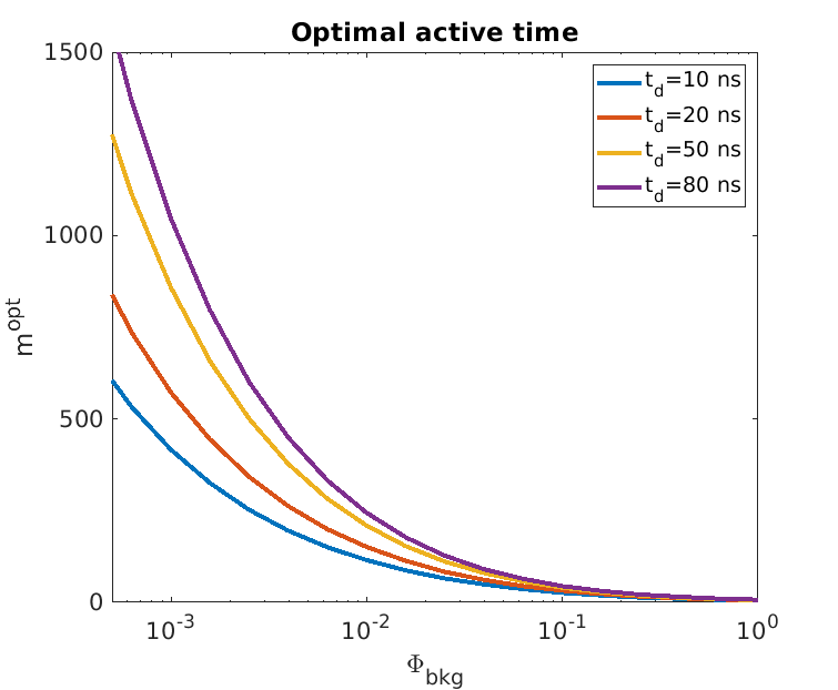
Supplementary Figure 1: Effect of ambient flux and dead time on $\bm{m}^{\text{opt}}$ . The optimal active time is a decreasing function of ambient flux $\Phi_{\text{bkg}}$ and an increasing function of dead time $t_{\text{d}}$.

In this section, we derive the optimal active time for uniform shifting. We assume that the expected denominator sequence is constant (achieved, say, using the method of laser and SPAD cycle mismatch from the previous section). Recall that we use an upper bound on the $\ell_{0}$ depth error as a surrogate for RMSE. From the proof of Result 1 we know that this is equivalent to using the smallest denominator sequence value as a surrogate for RMSE. However, since the denominator sequence is constant on average, we can use the total expected denominator $\Xi$ from Eq. (S7) as a surrogate for depth accuracy—a lower total expected denominator would correspond to higher depth errors and vice versa. We now derive the value of $m$ that maximizes $\Xi$.

Since the length of each SPAD cycle is $m\Delta+t_{\text{d}}$, the number of cycles in a fixed acquisition time $T$ is given by

$$L=\frac{T}{m\Delta+t_{\text{d}}}.$$ (S8)

From Eqs. (S7) and (S8), we get:

$$\Xi(m)=\frac{T}{m\Delta+t_{\text{d}}}\frac{1-e^{-m\Phi_{\text{bkg}}}}{1-e^{-\Phi_{\text{bkg}}}}.$$

where we have explicitly included the dependence of $\Xi$ on the active time $m$. Intuitively, the first term represents the average number of SPAD measurement cycles that can fit in time $T$ and the second term is the expected denominator value in each cycle (assumed to be uniform over all histogram bins in each cycle). The optimal active time $m^{\text{opt}}$ is the one that maximizes the total denominator. Solving for $\nicefrac{{d\Xi}}{{dm}}=0$, yields [Suppl. Ref. 5]:

$$m^{\text{opt}}=-\frac{1}{\Phi_{\text{bkg}}}\mathsf{LambertW}(-e^{-t_{\text{d}}\Phi_{\text{bkg}}/\Delta-1})-\frac{t_{\text{d}}}{\Delta}-\frac{1}{\Phi_{\text{bkg}}}.$$ (S9)

Interpreting $\bm{m}^{\text{opt}}$: Suppl. Fig. 1 shows the behavior of $m^{\text{opt}}$ for different values of dead time $t_{\text{d}}$ and varying ambient flux $\Phi_{\text{bkg}}$. Observe that the optimal active time decreases with increasing $\Phi_{\text{bkg}}$. Under high ambient photon flux, the average time until the first photon detection after the SPAD active time window begins is small. As a result, keeping the SPAD active for a longer duration is inefficient because it unnecessarily increases the length of the measurement cycle, and reduces the number of measurements that can be acquired over a fixed acquisition time. Conversely, at lower flux levels, the optimal active time increases to match the increased average inter-photon arrival time.

For a fixed background flux level, $m^{\text{opt}}$ is higher for longer dead times. When the dead time is long, increasing the active time duration increases the probability of detecting a photon while not increasing the measurement cycle length by much.

A uniform shift sequence with SPAD active time equal to $m^{\text{opt}}$ can be implemented using the method described in Supplementary Note 3.

Supplementary Note 5 Photon-Driven Shifting: Histogramming and Error Analysis

In this section we provide a proof of Result 3 which states that photon-driven shifting achieves a uniform shift sequence for sufficiently large acquisition times.

This section also proposes an algorithm for computing the generalized Coates’s estimator for photon-driven shifting. Unlike uniform shifting where the shift sequence is deterministic and can be pre-computed, the shift sequence in photon-driven shifting is random and depends on the actual photon detection times. We show how the arrival timestamps can be used to compute $D_{i}$ and $N_{i}$ needed for the generalized Coates’s estimator. It is also possible to estimate the waveform in free-running acquisition using a Markov chain-based model of the arrival times [Suppl. Ref. 6]. While the Markov chain-based estimator is based on solving a non-convex optimization problem, the proposed generalized Coates’s estimator has a closed-form expression. Both achieve equivalent performance in terms of depth recovery accuracy.

Proof of Result 3

Let $(S_{l})_{l=1}^{L}$ denote the stochastic shift sequence, where $0\leq S_{l}\leq B-1$ and $\ominus$ denote subtraction modulo-B with a wrap around when the index falls below $1$. This shift sequence forms a Markov chain with state space $[0,B-1]$ and transition density given by [Suppl. Ref. 6]:

$$f_{S_{i+1}|S_{i}}(s_{i+1}|s_{i})=\begin{cases}\left(\frac{1-e^{-\Phi_{\text{bkg}}}}{1-e^{-B\Phi_{\text{bkg}}}}\right)e^{-(s_{i+1}\ominus s_{i}+B-t_{d})\Phi_{\text{bkg}}}&\text{if }s_{i+1}\ominus s_{i}<t_{\text{d}}\\ \left(\frac{1-e^{-\Phi_{\text{bkg}}}}{1-e^{-B\Phi_{\text{bkg}}}}\right)e^{-(s_{i+1}\ominus s_{i}-t_{d})\Phi_{\text{bkg}}}&\text{otherwise.}\end{cases}$$

The uniform distribution $f(s)=\frac{1}{B}$ is a stationary distribution for this irreducible aperiodic Markov chain, and hence it converges to its stationary distribution [Suppl. Ref. 7] as $L\rightarrow\infty$. Let $f^{k}(s)$ denote the distribution of the $k^{\text{th}}$ shift. We have:

$$\lim_{k\to\infty}f^{k}(s)=f(s)$$

Therefore, as $L\rightarrow\infty$, the empirical distribution of $(s_{1},s_{2},\ldots,s_{L})\to f(s)$ and all shifts are achieved with equal probability making the shift sequence uniform. This also leads to a constant expected denominator sequence as shown in the simulations below.

Simulations: Suppl. Fig. 2 shows the expected denominator sequence for different total acquisition times at three different ambient flux levels. There are two main observations here. First, for short acquisition times there is a depth-dependent bias which disappears as $T$ increases. Second, for fixed $T$, the depth dependent bias is higher for higher flux levels. This is because at high ambient light, the SPAD detects a photon almost deterministically after each dead time window elapses which causes the Markov chain $(S_{l})_{l=1}^{L}$ to have a longer mixing time than at lower ambient flux levels.

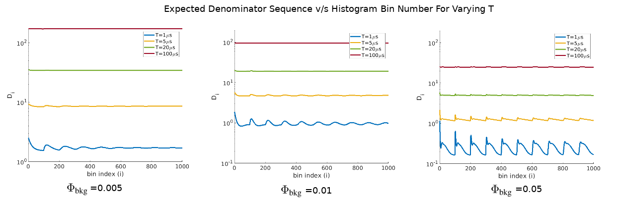
Supplementary Figure 2: Effect of flux and acquisition time on denominator sequence. The expected denominator sequence in the photon-driven mode has a position dependent bias which disappears as the total acquisition time increases.

Histogram and denominator sequence computation

In this section, we provide details about the algorithm for computing $N_{i}$ and $D_{i}$ from the shift sequence and the sequence of photon arrival times. This leads to a computationally tractable method for computing the generalized Coates’s estimate for the flux waveform and hence estimating scene depths.

Let $(u_{1},u_{2},\ldots,u_{L})$ denote the photon arrival times (in terms of bin index) in each SPAD cycle measured with respect to the most recent laser cycle. Note that $1\leq u_{i}\leq B$.

The histogram of photon counts is given by:

$$N_{i}=\sum_{l=1}^{L}\mathbbm{1}(u_{l}=i)$$

To compute the denominator sequence, we loop through the list of photon arrival times $u_{l}$. For each photon detection time we increment $D_{j}$ for every bin index $j\in J_{l,u_{l}}$.

In the photon-driven shifting mode, the denominator sequence can also be computed in closed form. The shift sequence $(s_{l})_{l=1}^{L}$ is determined by the photon arrival times $u_{i}$ as $s_{l+1}=u_{l}\oplus n_{d}$ where $n_{d}$ is the dead time in units of bins. As before, $N_{i}$ is given by the histogram of $(u_{l})_{l=1}^{L}$. $D_{i}$ can be computed in closed form in terms of the histogram counts: For each bin index $i$, there are $\frac{T}{B\Delta}$ depth bins in total which can potentially detect photons. However, a photon detection in any depth bin prohibits the $n_{d}$ bins that follow it from detecting photons. Therefore, the value of $D_{i}$ at the $i^{\text{th}}$ bin is given by subtracting these bins from the total:

$$D_{i}=\frac{T}{B\Delta}-\sum_{j=1}^{t_{d}/\Delta}N_{i\ominus j}.$$

As before for the case of deterministic shifting, the likelihood function of the photon incidence probabilities $(q_{i})_{i=1}^{B}$ is given by:

$$\mathcal{L}(q_{1},q_{2},...,q_{B})=\prod_{i=1}^{B+1}q_{i}^{N_{i}}(1-q_{i})^{D_{i}-N_{i}}\,.$$

Therefore, the generalized Coates’s estimator for photon-driven shifting is given as the following closed-form expression:

$$\widehat{\tau} =\operatorname*{arg\,max}_{i}\frac{N_{i}}{D_{i}}$$

$$=\operatorname*{arg\,max}_{i}\frac{N_{i}}{\frac{T}{B\Delta}-\sum_{j=1}^{t_{d}/\Delta}N_{i\ominus j}}\,.$$ (S10)

Markov chain model-based estimator [Suppl. Ref. 6]

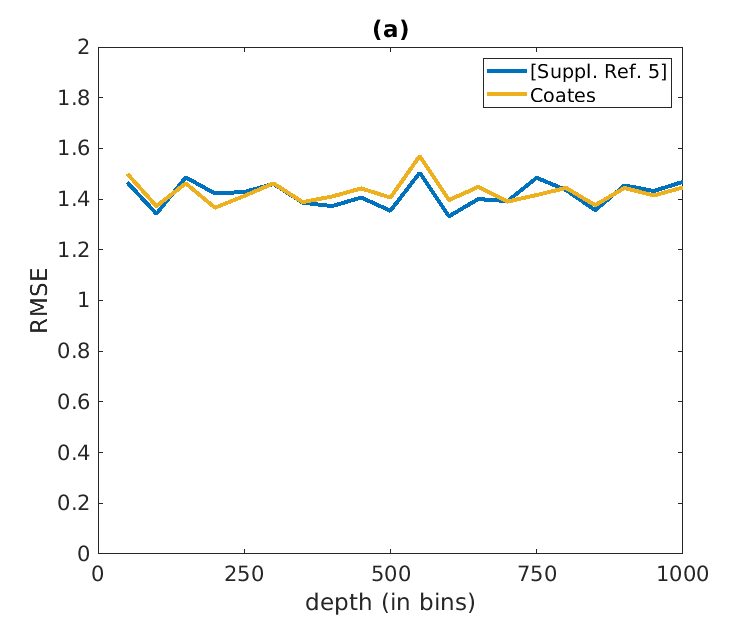
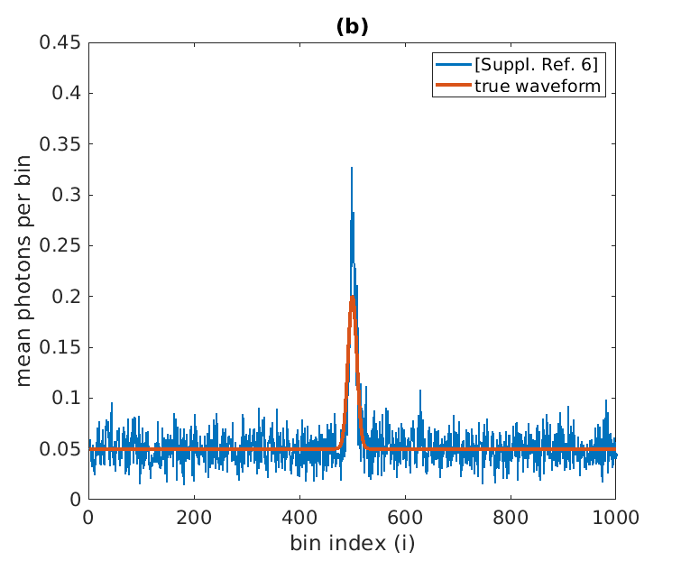
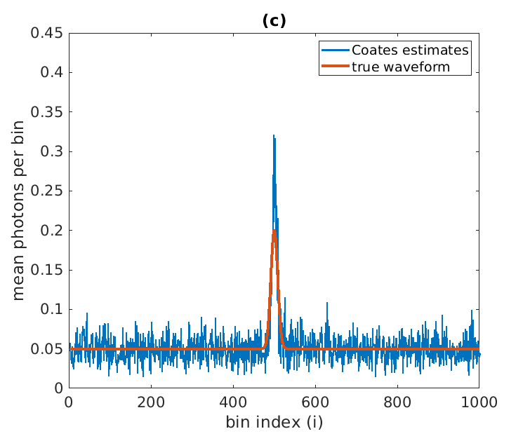
Supplementary Figure 3: Comparison between [Suppl. Ref. 6] and the proposed generalized Coates’s estimator. (a) shows the RMSE curve for the two methods. Both methods have the same performance across depth. (b) and (c) show that the estimated waveforms using the two methods are similar.

It is also possible to use a Markov chain for modeling the photon arrival times in free-running acquisition. The resulting estimator [Suppl. Ref. 6] is based on solving a non-convex optimization problem, whereas the proposed generalized Coates’s estimator has a closed-form expression, as shown above. Both achieve equivalent performance in terms of depth recovery accuracy, as shown in Suppl. Fig. 3. In the regime of large acquisition time ($T=$25\text{\,}\mathrm{\SIUnitSymbolMicro s}$$), and with $\Phi_{\text{bkg}}=0.05,\Phi_{\text{sig}}=0.15$, the performance of both the estimators in terms of depth error is almost equivalent.

Performance Gain as a Function of Depth

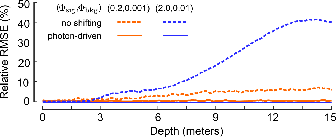
Supplementary Figure 4: Asynchronous acquisition schemes minimize overall depth error, and as a byproduct also provide uniform error with depth. The performance gain is larger at longer distances.

Suppl. Fig. 4 shows error vs. depth for photon-driven and conventional synchronous acquisition for different source and background flux levels. There are two key observations:

1. The performance gain from photon-driven acquisition is greater at longer distances. (Although not shown here, similar conclusion can be drawn for deterministic shifting as well.)

2. RMSE is approximately depth-invariant for photon-driven shifting.

Achieving uniform error over all depths is not our primary goal, but a byproduct of our optimal acquisition schemes. We define optimality in terms of a surrogate of $\ell_{2}$ depth error metric which measures overall depth error. Result 1 shows that the optimal acquisition scheme that minimizes our error metric also has a constant denominator sequence for all depths.

Supplementary Note 6 Asynchronous Shifting: Practitioner’s View

In this supplementary note we provide practical guidelines for design of asynchronous acquisition strategies. We provide a comparison between photon-driven shifting and uniform shifting with optimal active time $m^{\text{opt}}$ and show that there are certain regimes where photon-driven shifting has slightly worse error performance than uniform shifting. We also analyze the effect of number of SPAD cycles on depth error performance of photon-driven acquistion.

Derivation of Expected Denominator Sequence for Photon-Driven Acquisition

We consider a low SBR scenario with $r_{i}\approx\Phi_{\text{bkg}}$ for all $i$. Let $(D_{i})_{i=1}^{B}$ denote the denominator sequence obtained over $L$ SPAD cycles and a fixed acquisition time $T$. Since the length of each SPAD cycle is random, the number of cycles in time $T$ is also random. By the equivalence of the length of the active period of a cycle and its contribution to the total denominator, we have:

$$D_{1}+D_{2}+...+D_{B}=M_{1}+M_{2}+...+M_{L}$$

where $M_{i}$ is a random variable denoting the length of the $i^{\text{th}}$ measurement window. Note that the $M_{i}$’s are i.i.d. with a discrete exponential distribution:

$$P(M_{i}=k)=e^{-(k-1)\Phi_{\text{bkg}}}\left(1-e^{-\Phi_{\text{bkg}}}\right)$$

for $k=1,2,3,\ldots.$ Therefore, $\mathbb{E}[M_{i}]=\frac{1}{1-e^{-\Phi_{\text{bkg}}}}$. Taking expectation on both sides of the above equation, we get:

$$\mathbb{E}[D_{1}+D_{2}+...+D_{B}] =\mathbb{E}[M_{1}+M_{2}+...+M_{L}]$$ (S11)

$$\approx\mathbb{E}[L]\mathbb{E}[M_{i}]=\frac{\mathbb{E}[L]}{1-e^{-\Phi_{\text{bkg}}}}\,,$$ (S12)

where, we have assumed that $M_{i}$ and $L$ are approximately independent. We also have:

$$(M_{1}+t_{\text{d}})+(M_{2}+t_{\text{d}})+...+(M_{L}+t_{\text{d}})=T\,.$$

Taking the expectation on both sides and using Eq. (S12), we get:

$$\frac{\mathbb{E}[L]}{1-e^{-\Phi_{\text{bkg}}}}+\mathbb{E}[L]t_{\text{d}}=T$$

which implies that

$$\mathbb{E}[L]=\frac{T}{\frac{1}{1-e^{-\Phi_{\text{bkg}}}}+t_{\text{d}}}\,.$$

Combining with Eq. (S11), we get:

$$\mathbb{E}[D_{1}+D_{2}+...+D_{B}]=\frac{T}{1+(1-e^{-\Phi_{\text{bkg}}})t_{\text{d}}}\,.$$

From Result 3, we know that $\mathbb{E}[D_{i}]$ is constant $\forall\,i$ as $L\to\infty$. Under this assumption, we have for $1\leq i\leq B$:

$$\mathbb{E}[D_{i}]|_{\text{photon-driven}}=\frac{T}{B(1+(1-e^{-\Phi_{\text{bkg}}})t_{\text{d}})}.$$ (S13)

Comparing expected denominator sequences for uniform shifting and photon-driven shifting: Recall from Supplementary Note 4 the expected denominator sequence for uniform shifting is given by:

$$\mathbb{E}[D_{i}]|_{\text{uniform}}=\frac{T(1-e^{-m\Phi_{\text{bkg}}})}{B(m\Delta+t_{\text{d}})(1-e^{-\Phi_{\text{bkg}}})}.$$ (S14)

Observe that $\mathbb{E}[D_{i}]|_{\text{photon-driven}}>\mathbb{E}[D_{i}]|_{\text{uniform}}$ for all $m\geq 1$, $\Phi_{\text{bkg}}$ and $t_{\text{d}}$. To a first order approximation, the expected denominator sequence alone determines the depth estimation performance of the various techniques that we discussed. This suggests that photon-driven shifting should be always better than uniform shifting. However, in some cases, depending on the dead time and incident flux levels, deterministic shifting can outperform photon-driven acquisition. One such scenario is demonstrated in Suppl. Fig. 5 using both simulation and experimental results. At certain values of dead time, photon-driven shifting fails to achieve uniform shifts in the fixed acquistion time.

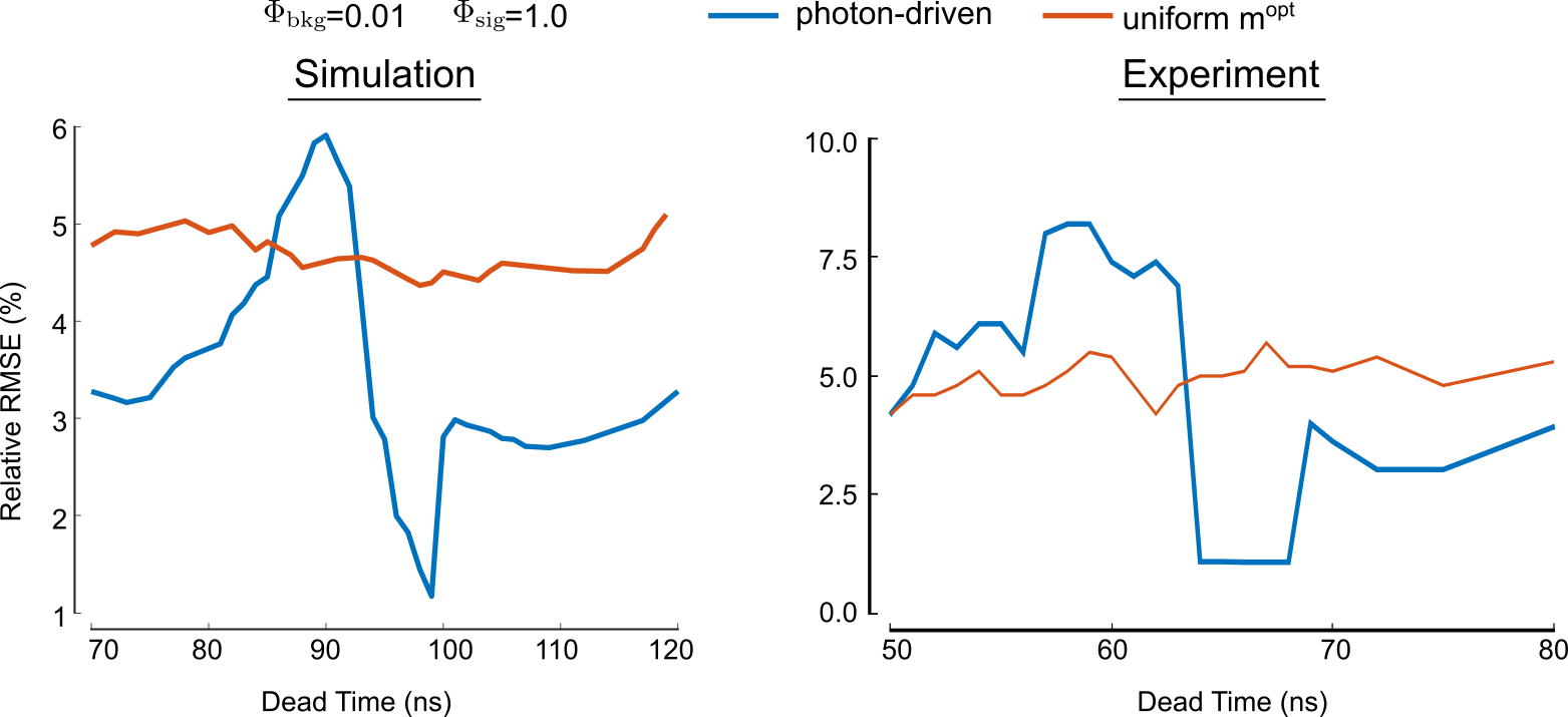
Supplementary Figure 5: In some special scenarios, depending on dead time and incident flux, uniform shifting may outperform photon-driven shifting.

Effect of reducing laser cycles on photon-driven shifting

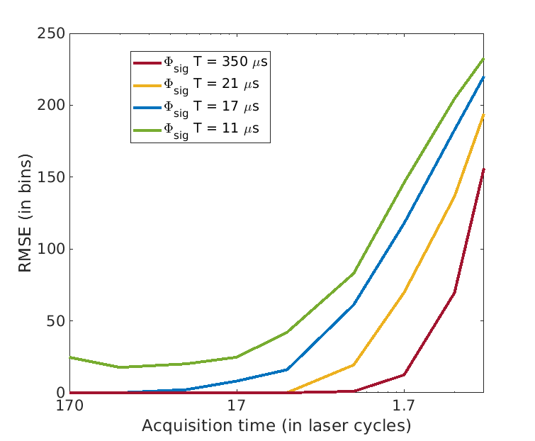
Supplementary Figure 6: Effect of reducing laser cycles on photon-driven shifting with optimal attenuation. Each curve has a fixed $\Phi_{\text{sig}}T$ product. As $T$ decreases and $\Phi_{\text{sig}}$ increases, the RMSE rises. The effect of decreasing $T$ can be overcome to some extent by increasing $\Phi_{\text{sig}}$.

Intuitively, one would expect asynchronous acquisition techniques to require a large number of cycles, in order to achieve uniform shifting and remove pileup as motivated in the main text. However, it turns out that our combined method of photon-driven shifting and optimal attenuation can work with very few laser cycles, provided that the signal flux is high. This is true even for relatively high ambient flux levels (we consider $\Phi_{\text{bkg}}=0.05$). Intuitively, even though uniform shifting cannot occur with laser cycles much less than the number of bins $B$, the combination of high effective $\Phi_{\text{sig}}$ and low effective $\Phi_{\text{bkg}}$ obviates the need for shifting.

In Suppl. Fig. 6, we evaluate depth error performance as number of laser cycles is decreased, while keeping the $\Phi_{\text{sig}}T$ product constant. For all $\Phi_{\text{sig}}$ levels, RMSE curves have flat valleys, with errors starting to rise beyond a certain $T$ and reaching the maximum possible error eventually. It is interesting to see the transition from the valley to max error for different $\Phi_{\text{sig}}$ levels. As the $\Phi_{\text{sig}}$ level is increased, the transition happens at a lower acquisition time, until $T$ becomes less than about $2$ laser cycles. Beyond this, the error cannot be reduced no matter how high $\Phi_{\text{sig}}$ is made. In some sense, this is the limiting point of our method.

Supplementary Note 7 Combining Shifting Strategies with Optimal Flux Attenuation

In this section we derive an expression for optimal flux attenuation for photon-driven acquisition. We also provide some information theoretic arguments for why it is important to combine asynchronous acquisition schemes with flux attenuation to achieve optimal depth error performance.

Optimal Attenuation Fraction for Photon-Driven Shifting

We will use similar techniques as the derivation of Result 1 from Supplementary Note 2 and introduce an additional variable $\Upsilon$ for flux attenuation fraction. In particular the expected denominator sequence in Eq. (S13) becomes:

$$\mathbb{E}[D_{i}]=\frac{T}{B(1+(1-e^{-\Upsilon\Phi_{\text{bkg}}})t_{\text{d}})}.$$ (S15)

From Eq. (Supplementary Note 2), we have:

$$\frac{1}{B}\sum_{\tau=1}^{B}\mathbb{P}(\widehat{\tau}\neq\tau) \leq\frac{1}{B}\sum_{i,\tau=1}^{B}\frac{1}{2}\exp{\left(-\frac{1}{2}\frac{(q_{\tau}-q_{i})^{2}}{\frac{q_{i}(1-q_{i})}{\mathbb{E}[D_{i}]}+\frac{q_{\tau}(1-q_{\tau})}{\mathbb{E}[D_{\tau}]}}\right)}$$

$$\approx\frac{1}{B}\sum_{i,\tau=1}^{B}\frac{1}{2}\exp{\left(-\frac{1}{2}{{\mathbb{E}[D_{i}]}(q_{\tau}-q_{i})}\right)}$$

$$=\frac{B}{2}\exp{\left(-\frac{1}{2}{{\mathbb{E}[D_{i}]}(q_{\tau}-q_{i})}\right)}$$

where in the second step, we have assumed that the denominator sequence is uniform, $q_{i},q_{\tau}\ll 1$ and $q_{\tau}-q_{i}\approx q_{\tau}+q_{i}$. Substituting Eq. (S15), the optimal attenuation fraction is given by:

$$\Upsilon^{\text{opt}} =\operatorname*{arg\,max}_{\Upsilon}\left[{\mathbb{E}[D_{i}]}(q_{\tau}-q_{i})\right]$$

$$=\operatorname*{arg\,max}_{\Upsilon}\frac{Te^{-\Upsilon\Phi_{\text{bkg}}}(1-e^{-\Upsilon\Phi_{\text{sig}}})}{B(1+(1-e^{-\Upsilon\Phi_{\text{bkg}}})t_{d})}.$$

The optimal attenuation fraction $\Upsilon^{\text{opt}}$ depends on various system parameters (number of bins, acquisition time and the dead time), which are known. $\Upsilon^{\text{opt}}$ also depends on the signal and background flux levels, which can be estimated a priori using a small number of laser cycles. Using the estimated values, the optimal flux attenuation can be determined, which can be used to further reduce the pile-up, and thus improve the depth estimation performance.

Fig. 6 in the main paper shows simulation results of depth RMSE for the conventional synchronous mode and photon-driven shifting over a range of attenuation factors and two different dead times. The locations of the minima agree with the theoretical expression derived above. There are two key observations that can be made from the figure. First, the optimal attenuation fraction with shifting is much higher than that for conventional synchronous acquisition. Second, combining attenuation with photon-driven shifting can provide a large gain in depth error performance, reducing the RMSE to almost zero for some combinations of SBR and dead time.

Information Theoretic Argument for Combining Shifting with Flux Attenuation

We formalize the notion of discriminative power of the histogram data for distinguishing between incident flux waveform levels using a concept from statistics called Fisher information [Suppl. Ref. 4, pp. 35]. This concept was also used in [Suppl. Ref. 6]. Fisher information measures of the rate of change of the likelihood function with respect to the unknown parameters $r_{i}$. For any attenuation coefficient $\Upsilon$, we can compute:

$$\mathcal{I}(r_{i};\Upsilon)=\mathbb{E}{\left[\left(\frac{\partial}{\partial r_{i}}\log\mathcal{L}(N_{i};D_{i},r_{i},\Upsilon)\right)^{2}\right]}$$

Substituting the expression for likelihood from Eq. (S5) and simplifying yields:

$$\mathcal{I}(r_{i};\Upsilon)=\frac{D_{i}\Upsilon^{2}}{e^{\Upsilon r_{i}}-1}$$ (S16)

Asynchronous acquisition methods can only change $D_{i}$ which appears in the numerator of the Fisher information. Attenuation can further increase the Fisher information and lead to better flux utilization than would be possible with shifting alone.

Supplementary Note 8 Details of Simulations and Experiments

Calculating RMSE

We calculate RMSE in a modulo-B sense in our simulations and experiments. For example, this means that the first and the last histogram bins are considered to be only $1$ bin apart. Let $M$ be the number of Monte Carlo runs, $B$ be the number of histogram bins, $\tau_{i}$ be the true depth bin index and $\widehat{\tau}_{i}$ be the estimated depth bin index for the $i^{\text{th}}$ Monte Carlo run. We calculate RMSE using the following formula:

$$\mathsf{RMSE}=\left[\frac{1}{M}\sum_{i=1}^{M}\left(\frac{B}{2}-\left(\widehat{\tau}_{i}-\tau_{i}+\frac{B}{2}\right)\,\mathsf{mod}\,B\right)^{2}\right]^{\frac{1}{2}}.$$

Monte Carlo Simulations

In Figs. 4 and 7, the dead time was $10\text{\,}\mathrm{ns}$, and the exposure time was $2.5\text{\,}\mathrm{\SIUnitSymbolMicro s}$ In Fig. 6, the exposure times were $2.5\text{\,}\mathrm{\SIUnitSymbolMicro s}$ and $2.9\text{\,}\mathrm{\SIUnitSymbolMicro s}$ respectively for the two dead times, to acquire an equal number of SPAD cycles in both cases. At low incident flux and longer dead times, an active time duration longer than $B$ may be needed to increase the probability that the SPAD captures a photon.

Experimental Setup

Suppl. Fig. 7 shows various components of our experimental setup. The SPAD is operated by a programmable control unit and photon timestamps are captured by a TCSPC module (not shown).

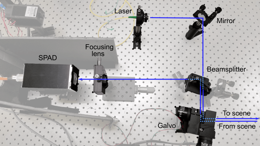
Supplementary Figure 7: Experimental setup The setup consists of a collimated pulsed laser and a single-pixel SPAD detector optically collocated using a beamsplitter. A pair of galvo mirrors scans the image plane and the light returning from the scene is focused on the detector using a focusing lens. The detector and focusing lens are enclosed in a light-tight box (not shown here) so that the all the light arriving at the detector pixel must pass through the lens.

Single-Pixel Experiment Results

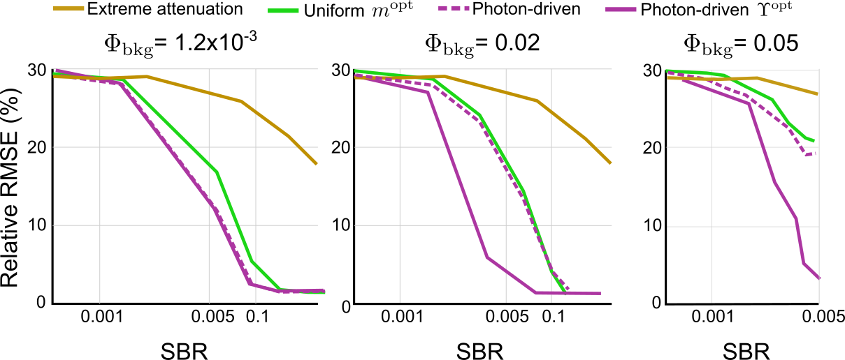
Supplementary Figure 8: RMSE in single-pixel experiments. Asynchronous schemes outperform the state-of-the-art method of synchronous acquisition with extreme attenuation at all flux levels. A combination of photon-driven shifting with optimal attenuation provides an order of magnitude lower RMSE at high ambient flux levels.

Suppl. Fig. 8 shows depth RMSE at four different ambient flux levels for a range of SBR values. A combination of photon-driven shifting with optimal attenuation provides the best performance of all techniques. For high ambient flux levels, even at high SBR, the conventional 5% rule-of-thumb and shifting alone fail to provide acceptable depth reconstruction performance. This suggests that the optimal acquisition strategy for SPAD-based LiDAR must use a combination of both shifting and attenuation.

Additional Result Showing Effect of Number of SPAD Cycles

Supplementary Figure 9: Depth reconstructions for varying number of SPAD cycles for “Reindeer” scene. Observe that the reconstruction accuracy improves as the number of cycles increases. Photon-driven shifting provides better reconstruction performance than all synchronous acquisition schemes. The source flux $\Phi_{\text{sig}}=0.5$ and ambient flux $\Phi_{\text{bkg}}=0.01$ for this experiment which corresponds to an SBR of 50.

Supplementary References

1. K. Murphy, Machine Learning: A Probabilistic Perspective. Cambridge, MA: MIT Press, 2012, pp. 35.

2. C. Daskalakis, G. Kamath, and C. Tzamos. On the structure, covering, and learning of poisson multinomial distributions. arXiv preprint, 2015.

3. A. Gupta, A. Ingle, A. Velten, and M. Gupta. Photon flooded single-photon 3d cameras. arXiv preprint arXiv:1903.08347, 2019.

4. S. Kay, Fundamentals of Statistical Signal Processing: Estimation Theory. Upper Saddle River, NJ: Prentice Hall, 1993, pp. 173–174.

5. R. M. Corless, G. H. Gonnet, D. E. G. Hare, D. J. Jeffrey, and D. E. Knuth. On the LambertW function. Advances in Computational Mathematics, 5(1):329–359, Dec 1996.

6. J. Rapp, Y. Ma, R. Dawson, and V. K. Goyal. Dead time compensation for high-flux ranging. arXiv preprint arXiv:1810.11145, 2018.

7. G. Grimmett, D. Stirzaker, Probability and Random Processes. Oxford, UK: Oxford University Press, 2001, pp. 227.

References

- [1] Giulia Acconcia, Alessandro Cominelli, Massimo Ghioni, and Ivan Rech. Fast fully-integrated front-end circuit to overcome pile-up limits in time-correlated single photon counting with single photon avalanche diodes. Opt. Express, 26(12):15398–15410, Jun 2018.
- [2] Wolfgang Becker. Advanced time-correlated single photon counting applications, volume 111. Springer, 2015.
- [3] Maik Beer, Jan Haase, Jennifer Ruskowski, and Rainer Kokozinski. Background light rejection in spad-based lidar sensors by adaptive photon coincidence detection. Sensors, 18(12):4338, Dec 2018.
- [4] Claudio Bruschini, Harald Homulle, Ivan Michel Antolovic, Samuel Burri, and Edoardo Charbon. Single-photon spad imagers in biophotonics: Review and outlook. arXiv preprint, 2019.
- [5] Samuel Burri, Yuki Maruyama, Xavier Michalet, Francesco Regazzoni, Claudio Bruschini, and Edoardo Charbon. Architecture and applications of a high resolution gated SPAD image sensor. Optics Express, 22(14):17573, Jul 2014.
- [6] Mauro Buttafava, Gianluca Boso, Alessandro Ruggeri, Alberto Dalla Mora, and Alberto Tosi. Time-gated single-photon detection module with 110 ps transition time and up to 80 mhz repetition rate. Review of Scientific Instruments, 85(8):083114, 2014.
- [7] Mauro Buttafava, Jessica Zeman, Alberto Tosi, Kevin Eliceiri, and Andreas Velten. Non-line-of-sight imaging using a time-gated single photon avalanche diode. Optics express, 23(16):20997–21011, 2015.
- [8] P. B. Coates. The correction for photon ‘pile-up’ in the measurement of radiative lifetimes. Journal of Physics E: Scientific Instruments, 1(8):878, 1968.
- [9] Alessandro Cominelli, Giulia Acconcia, Pietro Peronio, Massimo Ghioni, and Ivan Rech. High-speed and low-distortion solution for time-correlated single photon counting measurements: A theoretical analysis. Review of Scientific Instruments, 88(12):123701, Dec 2017.
- [10] Constantinos Daskalakis, Gautam Kamath, and Christos Tzamos. On the structure, covering, and learning of poisson multinomial distributions. arXiv preprint, 2015.
- [11] Neale A. W. Dutton, Istvan Gyongy, Luca Parmesan, Salvatore Gnecchi, Neil Calder, Bruce R. Rae, Sara Pellegrini, Lindsay A. Grant, and Robert K. Henderson. A SPAD-based QVGA image sensor for single-photon counting and quanta imaging. IEEE Transactions on Electron Devices, 63(1):189–196, Jan 2016.
- [12] Abhiram Gnanasambandam, Omar Elgendy, Jiaju Ma, and Stanley H Chan. Megapixel photon-counting color imaging using quanta image sensor. Optics Express, 27(12):17298–17310, 2019.
- [13] Anant Gupta, Atul Ingle, Andreas Velten, and Mohit Gupta. Photon-flooded single-photon 3d cameras. In Proceedings of the IEEE CVPR, pages 6770–6779, 2019.
- [14] Felix Heide, Steven Diamond, David Lindell, and Gordon Wetzstein. Sub-picosecond photon-efficient 3d imaging using single-photon sensors. Scientific Reports, 8(1), Dec 2018.
- [15] Atul Ingle, Andreas Velten, and Mohit Gupta. High flux passive imaging with single photon sensors. In Proc. CVPR, June 2019.
- [16] Sebastian Isbaner, Narain Karedla, Daja Ruhlandt, Simon Christoph Stein, Anna Chizhik, Ingo Gregor, and Jörg Enderlein. Dead-time correction of fluorescence lifetime measurements and fluorescence lifetime imaging. Optics express, 24(9):9429–9445, 2016.
- [17] Peter Kapusta, Michael Wahl, and Rainer Erdmann. Advanced Photon Counting Applications, Methods, Instrumentation. Springer Series on Fluorescence, 15, 2015.
- [18] Myung-Jae Lee and Edoardo Charbon. Progress in single-photon avalanche diode image sensors in standard cmos: From two-dimensional monolithic to three-dimensional-stacked technology. Japanese Journal of Applied Physics, 57(10):1002A3, 2018.
- [19] David Lindell, Matthew O’Toole, and Gordon Wetzstein. Single-Photon 3D Imaging with Deep Sensor Fusion. ACM Trans. Graph. (SIGGRAPH), 37(4), 2018.
- [20] Jiaju Ma, Saleh Masoodian, Dakota A Starkey, and Eric R Fossum. Photon-number-resolving megapixel image sensor at room temperature without avalanche gain. Optica, 4(12):1474–1481, 2017.
- [21] Matthew O’Toole, Felix Heide, David Lindell, Kai Zang, Steven Diamond, and Gordon Wetzstein. Reconstructing transient images from single-photon sensors. In 2017 IEEE Conference on Computer Vision and Pattern Recognition (CVPR), pages 2289–2297, July 2017.
- [22] Matthew O’Toole, David B. Lindell, and Gordon Wetzstein. Confocal non-line-of-sight imaging based on the light-cone transform. Nature, 555:338–341, Mar 2018.
- [23] Matthias Patting, Paja Reisch, Marcus Sackrow, Rhys Dowler, Marcelle Koenig, and Michael Wahl. Fluorescence decay data analysis correcting for detector pulse pile-up at very high count rates. Optical engineering, 57(3):031305, 2018.
- [24] Agata M. Pawlikowska, Abderrahim Halimi, Robert A. Lamb, and Gerald S. Buller. Single-photon three-dimensional imaging at up to 10 kilometers range. Optics Express, 25(10):11919, May 2017.
- [25] Adithya K Pediredla, Aswin C Sankaranarayanan, Mauro Buttafava, Alberto Tosi, and Ashok Veeraraghavan. Signal processing based pile-up compensation for gated single-photon avalanche diodes. arXiv preprint arXiv:1806.07437, 2018.
- [26] Sara Pellegrini, Gerald S Buller, Jason M Smith, Andrew M Wallace, and Sergio Cova. Laser-based distance measurement using picosecond resolution time-correlated single-photon counting. Measurement Science and Technology, 11(6):712, 2000.
- [27] Joshua Rapp and Vivek Goyal. A few photons among many: Unmixing signal and noise for photon-efficient active imaging. IEEE Transactions on Computational Imaging, 3(3):445–459, Sept 2017.
- [28] Joshua Rapp, Yanting Ma, Robin Dawson, and Vivek K Goyal. Dead time compensation for high-flux ranging. arXiv preprint arXiv:1810.11145, 2018.
- [29] Daniel Reilly and Gregory Kanter. High speed lidar via GHz gated photon detector and locked but unequal optical pulse rates. Optics Express, 22(13):15718, jun 2014.
- [30] Alexis Rochas. Single Photon Avalanche Diodes in CMOS Technology. PhD thesis, EPFL, 2003.
- [31] Alberto Tosi, Alberto Dalla Mora, Franco Zappa, Angelo Gulinatti, Davide Contini, Antonio Pifferi, Lorenzo Spinelli, Alessandro Torricelli, and Rinaldo Cubeddu. Fast-gated single-photon counting technique widens dynamic range and speeds up acquisition time in time-resolved measurements. Optics Express, 19(11):10735, May 2011.
- [32] Arin Can Ulku, Claudio Bruschini, Ivan Michel Antolovic, Yung Kuo, Rinat Ankri, Shimon Weiss, Xavier Michalet, and Edoardo Charbon. A 512x512 spad image sensor with integratedgating for widefield flim. IEEE Journal of Selected Topics in Quantum Electronics, 25(1):1–12, Jan 2019.
- [33] Michael Wahl. Time-Correlated Single Photon Counting, 2016.
- [34] Xue Feng Wang, Teruo Uchida, David M. Coleman, and Shigeo Minami. A two-dimensional fluorescence lifetime imaging system using a gated image intensifier. Applied Spectroscopy, 45(3):360–366, mar 1991.
- [35] Chao Zhang, Scott Lindner, Ivan Antolovic, Martin Wolf, and Edoardo Charbon. A CMOS SPAD Imager with Collision Detection and 128 Dynamically Reallocating TDCs for Single-Photon Counting and 3D Time-of-Flight Imaging. Sensors, 18(11):4016, Nov 2018.
Supplementary Document for