Quantum Ornstein-Zernike Equation

Abstract

The non-commutativity of the position and momentum operators is formulated as an effective potential in classical phase space and expanded as a series of successive many-body terms, with the pair term being dominant. A non-linear partial differential equation in temperature and space is given for this. The linear solution is obtained explicitly, which is valid at high and intermediate temperatures, or at low densities. An algorithm for solving the full non-linear problem is given. Symmetrization effects accounting for particle statistics are also written as a series of effective many-body potentials, of which the pair term is dominant at terrestrial densities. Casting these quantum functions as pair-wise additive, temperature-dependent, effective potentials enables the established techniques of classical statistical mechanics to be applied to quantum systems. The quantum Ornstein-Zernike equation is given as an example.

I Introduction

WignerWigner32 gave a formulation of quantum statistical mechanics that expressed the probability density for classical phase space as a multi-dimensional convolution integral of the Maxwell-Boltzmann operator acting on the momentum eigenfunctions. He used this expression to obtain the primary quantum correction to the classical free energy, which was of second order in Planck’s constant for an unsymmetrized wave function. KirkwoodKirkwood33 showed that the temperature derivative of Wigner’s integrand was slightly more convenient for developing expansions in powers of either Plank’s constant or of inverse temperature. He used it to give both the first and second order quantum corrections to the classical result for a symmetrized wave function.

I also have developed a formulation of quantum statistical mechanics in classical phase space. STD2 ; Attard18a This eschews Wigner’s convolution integral, but it nevertheless involves the same Maxwell-Boltzmann operator acting on the momentum eigenfunctions. I have named this phase function the commutation function, because it accounts for the non-commutativity of the position and momentum operators that is otherwise neglected in classical mechanics. Using Kirkwood’s temperature derivative method, I have obtained the quantum corrections up to and including fourth order in Plank’s constant.STD2 ; Attard18b The coefficients involve gradients of the potential energy, and their number and complexity grows exponentially for successive terms in the expansion. Whilst undoubtedly useful at high temperatures, where all systems are predominantly classical, at intermediate and low temperatures the series expansion is tedious to derive, complex to program, and slow to converge, and it does not appear to be a practical approach for condensed matter systems.

An alternative approach is based upon a formally exact transformation that expresses the commutation function as a sum over energy eigenvalues and eigenfunctions.Attard18c Although these are not known explicitly for a general system, they are known exactly for the simple harmonic oscillator. Accordingly, in a mean field approach the commutation function for a point in classical phase space can be approximated by that of a simple harmonic oscillator based on a second order expansion of the potential about the nearest local minimum for the configuration. A Metropolis Monte Carlo simulation using this mean field–simple harmonic oscillator approximation has been shown to yield accurate results at low temperatures for two condensed matter systems where the quantum result is known to high accuracy: a Lennard-Jones fluid,Hernando13 ; Attard18c and an harmonic crystal.Attard19

A big advantage of the classical phase space formulation of quantum statistical mechanics in general is that the required computer time for a given statistical accuracy scales sub-linearly with system size. However the difficulty with the mean field–simple harmonic oscillator approximation is that one cannot be certain of its accuracy in the absence of benchmark results for the same specific system. Although the mean field aspect has been improved by applying it at the pair level,Attard19 it is unclear how to go beyond approximating the commutation function as that of an effective simple harmonic oscillator. Whilst undoubtedly there are strong arguments in favor of mean field approaches in condensed matter, there is some motivation to develop a more systematic approach to evaluating the commutation function, but without the tedium of the crude expansions as derived by Wigner,Wigner32 by Kirkwood,Kirkwood33 and by me.Attard18b

This paper makes a significant advance with a new, systematic expansion for the commutation function. The explicit contributions are fewer and simpler than in the high temperature or Planck’s constant expansions, while the approach avoids the ad hoc nature of the mean field–simple harmonic oscillator approximation.

Here the commutation function is written as an effective potential, which is then expanded as a formal series of singlet, pair, three-body functions etc. Postulating that the many body terms are often negligible, only the pair commutation function needs to be retained for the common case of a homogeneous system. This is a function of the relative separations and the relative momenta summed over all particle pairs. A non-linear partial differential equation is given for its temperature derivative and spatial gradients. An explicit solution is obtained in Fourier space for the linearized equations, which are valid at high and intermediate temperatures, and also at large separations. This provides a convenient starting point for the full non-linear solution via step-wise integration down to low temperatures, if required. As part of a computational algorithm, the full solution for the pair function can be stored on a three-dimensional grid prior to the commencement of, say, a Monte Carlo computer simulation, where it can be conveniently evaluated by interpolation from the storage grid. Beyond computer simulations, casting the quantum commutation function as a temperature-dependent, effective potential lends itself to the standard analytic techniques of classical statistical mechanics such as density functional theory, diagrammatic expansion, integral equation methods, asymptotic analysis, etc. As an example, the quantum Ornstein-Zernike equation is given.

II Analysis

II.1 Phase Space Formulation of Quantum Statistical Mechanics

The classical phase space quantum probability density for the canonical equilibrium system is (see Refs [STD2, ; Attard18a, ] and also Appendix A)

$$\wp({\bf p},{\bf q})=\frac{e^{-\beta{\cal H}({\bf p},{\bf q})}}{N!h^{3N}Z(T)}\,\omega({\bf p},{\bf q})\,\eta^{\pm}({\bf p},{\bf q}).$$ (2.1)

Here $N$ is the number of particles, ${\bf p}=\{{\bf p}_{1},{\bf p}_{2},\ldots,{\bf p}_{N}\}$ are their momenta, with ${\bf p}_{j}=\{p_{jx},p_{jy},p_{jz}\}$ being the momentum of the $j$th particle (three dimensional space is assumed), ${\bf q}=\{{\bf q}_{1},{\bf q}_{2},\ldots,{\bf q}_{N}\}$ are the positions, $\beta=1/k_{\mathrm{B}}T$ is the inverse temperature, with $T$ the temperature and $k_{\mathrm{B}}$ Boltzmann’s constant, and $h$ is Planck’s constant. The classical Hamiltonian is ${\cal H}({\bf p},{\bf q})={\cal K}({\bf p})+U({\bf q})$, with ${\cal K}=p^{2}/2m$ being the kinetic energy, and $U$ being the potential energy. The partition function $Z(T)$ normalizes the phase space probability density. The distinctly quantum aspects of the system are embodied in the symmetrization function $\eta$ and the commutation function $\omega$. Although it is straightforward to treat particle spin,Attard19 in this paper it is not included.

The symmetrization and commutation functions are defined in terms of the unsymmetrized position and momentum eigenfunctions, which in the position representation are respectivelyMessiah61

$$|{\bf q}\rangle=\delta({\bf r}-{\bf q}),\mbox{ and }|{\bf p}\rangle=\frac{e^{-{\bf p}\cdot{\bf r}/i\hbar}}{V^{N/2}}.$$ (2.2)

Here $\hbar=h/2\pi$, and $V$ is the volume of the system.

The symmetrization function is formallyAttard18a ; Attard19

$$\eta^{\pm}({\bf p},{\bf q})\equiv\frac{1}{\langle{\bf p}|{\bf q}\rangle}\sum_{\hat{\mathrm{P}}}(\pm 1)^{p}\,\langle\hat{\mathrm{P}}{\bf p}|{\bf q}\rangle,$$ (2.3)

with $\hat{\mathrm{P}}$ the permutation operator and $p$ its parity. The plus sign is for bosons and the minus sign is for fermions.

A pair-wise additive form of the symmetrization function is given in §II.4. See earlier work for the derivation of the phase space probability density, STD2 ; Attard18a and for the proof that the symmetrization factor correctly accounts for boson and fermion statistics.Attard19 ; FN1

II.2 Commutation Function

The commutation function $\omega$, which is essentially the same as the functions introduced by WignerWigner32 and analyzed by Kirkwood,Kirkwood33 is defined by

$$e^{-\beta{\cal H}({\bf p},{\bf q})}\omega({\bf p},{\bf q})=\frac{\langle{\bf q}|e^{-\beta\hat{\cal H}}|{\bf p}\rangle}{\langle{\bf q}|{\bf p}\rangle}.$$ (2.4)

The departure from unity of the commutation function reflects the non-commutativity of the position and momentum operators. To see this simply note that if position and momentum commuted, then the Maxwell-Boltzmann operator would factorize, $e^{-\beta\hat{\cal H}({\bf r})}=e^{-\beta U({\bf r})}e^{-\beta\hat{\cal K}({\bf r})}$. Then since $e^{-\beta\hat{\cal K}}|{\bf p}\rangle=e^{-\beta{\cal K}({\bf p})}|{\bf p}\rangle$, the right hand side would reduce to the classical Maxwell-Boltzmann factor $e^{-\beta{\cal H}({\bf p},{\bf q})}$, in which case $\omega({\bf p},{\bf q})=1$.

Obviously the system must become classical in the high temperature limit, and so $\omega({\bf p},{\bf q})\rightarrow 1$, $\beta\rightarrow 0$.

Further, the potential energy decays to zero at large separations, and the gradients of the potential are negligible compared to the potential itself. This means that at large separations the potential energy and the kinetic energy operator effectively commute, and so one similarly must have $\omega({\bf p},{\bf q})\rightarrow 1$, all $q_{jk}\rightarrow\infty$.

Following Kirkwood,Kirkwood33 differentiation of the defining equation with respect to inverse temperature givesSTD2

$$\frac{\partial\omega}{\partial\beta} = \frac{-\beta\hbar^{2}}{2m}(\nabla^{2}U)\omega-\frac{\beta\hbar^{2}}{m}(\nabla U)\cdot(\nabla\omega)$$ (2.5)

$$\mbox{ }+\frac{\beta^{2}\hbar^{2}}{2m}(\nabla U)\cdot(\nabla U)\omega+\frac{\hbar^{2}}{2m}\nabla^{2}\omega$$

$$\mbox{ }+\frac{i\hbar}{m}{\bf p}\cdot(\nabla\omega)-\frac{i\hbar\beta}{m}{\bf p}\cdot(\nabla U)\omega.$$

One can see from this that since $\nabla U\rightarrow 0$ at large separations, the putative asymptote, $\omega({\bf p},{\bf q})\rightarrow 1$, makes the right hand side vanish, which is consistent with the asymptote being a temperature-independent constant. This partial differential equation provides the basis for the high temperature expansions that were mentioned in the introduction. Wigner32 ; Kirkwood33 ; STD2 ; Attard18b The multiplicity of gradients on the right hand side is the origin for the rapid increase of number and complexity of the contributions to each order of the expansions, which are listed in Appendix B.

Elsewhere I have argued that it is more useful to cast the commutation function as an effective potential, STD2

$$W({\bf p},{\bf q})\equiv\ln\omega({\bf p},{\bf q}),\mbox{ or }\omega({\bf p},{\bf q})\equiv e^{W({\bf p},{\bf q})}.$$ (2.6)

(The present notation differs from previous articles.) In this form $W$ is a temperature-dependent effective potential. The original rationale for this was that $W$ is extensive with system size, which is an exceedingly useful property in thermodynamics. It was also hoped that the expansion of $W$ in powers of Planck’s constant or inverse temperature might have better convergence properties than those of $\omega$ itself, a hope more happy in prospect than in actual experience.

II.3 Many Body Expansion

The effective potential $W$ provides the starting point for the new approach to the commutation function, which is the main point of this paper.

Defining $\tilde{W}\equiv W-\beta U$, the temperature derivative of the definition leads toSTD2

$$\frac{\partial\tilde{W}}{\partial\beta}=-{\cal H}+\frac{i\hbar}{m}{\bf p}\cdot\nabla\tilde{W}+\frac{\hbar^{2}}{2m}\nabla^{2}\tilde{W}+\frac{\hbar^{2}}{2m}\nabla\tilde{W}\cdot\nabla\tilde{W},$$ (2.7)

with $\tilde{W}\sim-\beta{\cal H}$, $\beta\rightarrow 0$. The right hand side contains two terms linear in $\tilde{W}$ and one non-linear, quadratic term.

In general the potential energy is the sum of one-body, two-body, three-body etc. potentials,

$$U({\bf q}) = \sum_{j=1}^{N}u^{(1)}({\bf q}_{j})+\sum_{j<k}^{N}u^{(2)}({\bf q}_{j},{\bf q}_{k})$$ (2.8)

$$\mbox{ }+\sum_{j<k<\ell}^{N}u^{(3)}({\bf q}_{j},{\bf q}_{k},{\bf q}_{\ell})+\ldots$$

In this work three-body and higher potentials will be neglected. It will also be assumed that there is no one-body potential, that the system is homogeneous, and that the pair potential is a function only of separation,

$$U({\bf q})=\sum_{j<k}^{N}u(q_{jk})=\frac{1}{2}\sum_{j,k}\!^{(k\neq j)}u(q_{jk}),$$ (2.9)

where the particle separation is $q_{jk}=|{\bf q}_{j}-{\bf q}_{k}|$.

For the effective potential form of the commutation function, a similar many body decomposition can be formally made, with momentum now being included

$$W({\bf p},{\bf q})$$

$$= \sum_{j=1}^{N}w^{(1)}({\bf p}_{j},{\bf q}_{j})+\sum_{j<k}^{N}w^{(2)}({\bf p}_{j},{\bf q}_{j};{\bf p}_{k},{\bf q}_{k})$$

$$\mbox{ }+\sum_{j<k<\ell}^{N}w^{(3)}({\bf p}_{j},{\bf q}_{j};{\bf p}_{k},{\bf q}_{k};{\bf p}_{\ell},{\bf q}_{\ell})+\ldots$$

For the homogeneous case, the singlet contribution vanishes, ($W^{(1)}=0$, $\tilde{W}^{(1)}=-\beta{\cal K}({\bf p})$, and $\nabla\tilde{W}^{(1)}={\bf 0}$), and the three-body and higher contributions, will be neglected. Assuming homogeneity, the pair commutation function for particles $j$ and $k$ is a function of the magnitudes of the relative momentum and separation, and the angle between them, $w^{(2)}(p_{jk},q_{jk},\theta_{jk})$. Alternatively, the relative momentum can be aligned with the $z$ axis, ${\bf p}_{jk}=p_{jk}\hat{\bf z}$, and the separation can be rotated to the $xz$-plane, $w^{(2)}(p_{jk},q_{jk,x},q_{jk,z})$, or $w^{(2)}(p,q_{\perp},q_{\parallel})$. In any case the commutation function that will be considered here is

$$W({\bf p},{\bf q})=\sum_{j<k}^{N}w^{(2)}({\bf p}_{jk},{\bf q}_{jk})=\frac{1}{2}\sum_{j,k}\!^{(k\neq j)}w^{(2)}_{jk}.$$ (2.11)

Inserting this pair ansatz into the temperature derivative equation, one sees that the left hand side, and the constant and linear terms on the right hand side, are all the sum of pair functions. However the non-linear quadratic term on the right hand side is

$$\nabla\tilde{W}\cdot\nabla\tilde{W}$$ (2.12)

$$= \sum_{\ell}\nabla_{\ell}\tilde{W}\cdot\nabla_{\ell}\tilde{W}$$

$$= \frac{1}{4}\sum_{\ell}\sum_{j,k}\!^{(k\neq j)}\sum_{j^{\prime},k^{\prime}}\!^{(k^{\prime}\neq j^{\prime})}\nabla_{\ell}\tilde{w}^{(2)}_{jk}\cdot\nabla_{\ell}\tilde{w}^{(2)}_{j^{\prime}k^{\prime}}$$

$$= \frac{1}{4}\sum_{\ell,k,k^{\prime}}\!^{(k,k^{\prime}\neq\ell)}\nabla_{\ell}\tilde{w}^{(2)}_{\ell k}\cdot\nabla_{\ell}\tilde{w}^{(2)}_{\ell k^{\prime}}$$

$$\mbox{ }+\frac{1}{4}\sum_{j,\ell,k^{\prime}}\!^{(j,k^{\prime}\neq\ell)}\nabla_{\ell}\tilde{w}^{(2)}_{j\ell}\cdot\nabla_{\ell}\tilde{w}^{(2)}_{\ell k^{\prime}}$$

$$\mbox{ }+\frac{1}{4}\sum_{\ell,k,j^{\prime}}\!^{(k,j^{\prime}\neq\ell)}\nabla_{\ell}\tilde{w}^{(2)}_{\ell k}\cdot\nabla_{\ell}\tilde{w}^{(2)}_{j^{\prime}\ell}$$

$$\mbox{ }+\frac{1}{4}\sum_{\ell,j,j^{\prime}}\!^{(j,j^{\prime}\neq\ell)}\nabla_{\ell}\tilde{w}^{(2)}_{j\ell}\cdot\nabla_{\ell}\tilde{w}^{(2)}_{j^{\prime}\ell}$$

$$= \sum_{j,k,k^{\prime}}\!^{(k,k^{\prime}\neq j)}\nabla_{j}\tilde{w}^{(2)}_{jk}\cdot\nabla_{j}\tilde{w}^{(2)}_{jk^{\prime}}.$$

This is in essence a three-body term. However, to the extent that the ‘force’ on particle $j$ due to particle $k$ is uncorrelated with that due to $k^{\prime}$, $k^{\prime}\neq k$, the sum of forces over $k^{\prime}$ may be argued to be small, perhaps averaging to zero. In this case the $k^{\prime}=k$ terms dominate, and this becomes

$$\nabla\tilde{W}\cdot\nabla\tilde{W} \approx \sum_{j,k}\!^{(k\neq j)}\nabla_{j}\tilde{w}^{(2)}_{jk}\cdot\nabla_{j}\tilde{w}^{(2)}_{jk}$$ (2.13)

$$= 2\sum_{j<k}\nabla_{j}\tilde{w}^{(2)}_{jk}\cdot\nabla_{j}\tilde{w}^{(2)}_{jk}.$$

This is now a two-body term, which is expected to be accurate at low densities and high temperatures where correlations are reduced. The two-body solution can test the magnitude of the neglected three-body terms, and successively improve the pairwise additive approximation.

Applying the pair ansatz to the temperature derivative, equating both sides term by term, and dropping the superscript $(2)$, one obtains

$$\frac{\partial\tilde{w}_{jk}}{\partial\beta} = -u_{jk}+\frac{i\hbar}{m}{\bf p}_{jk}\cdot\nabla_{j}\tilde{w}_{jk}+\frac{\hbar^{2}}{m}\nabla_{j}^{2}\tilde{w}_{jk}$$ (2.14)

$$\mbox{ }+\frac{\hbar^{2}}{m}\nabla_{j}\tilde{w}_{jk}\cdot\nabla_{j}\tilde{w}_{jk}.$$

Here and above the symmetry $\tilde{w}_{jk}=\tilde{w}_{kj}$ has been exploited. Note that $\tilde{w}_{jk}\sim-\beta u_{jk}$, $\beta\rightarrow 0$.

Write ${\bf p}_{jk}=p_{z}\hat{\bf z}$, and ${\bf q}_{jk}=q_{x}\hat{\bf x}+q_{z}\hat{\bf z}$, and $q_{jk}=\sqrt{q_{x}^{2}+q_{z}^{2}}$. This then becomes

$$\frac{\partial\tilde{w}(p_{z},q_{x},q_{z})}{\partial\beta} = -u(q)+\frac{i\hbar}{m}p_{z}\tilde{w}_{z}+\frac{\hbar^{2}}{m}\left\{\tilde{w}_{xx}+\tilde{w}_{zz}\right\}$$ (2.15)

$$\mbox{ }+\frac{\hbar^{2}}{m}\left\{\tilde{w}_{x}^{2}+\tilde{w}_{z}^{2}\right\}.$$

The subscripts on $\tilde{w}$ signify spatial derivatives.

Define the two dimensional Fourier transform pair

$$\hat{\tilde{w}}(p_{z},k_{x},k_{y}) = \int\mathrm{d}{\bf q}\;e^{-i{\bf k}\cdot{\bf q}}\tilde{w}(p_{z},q_{x},q_{z})$$ (2.16)

$$\tilde{w}(p_{z},q_{x},q_{z}) = \frac{1}{(2\pi)^{2}}\int\mathrm{d}{\bf k}\;e^{i{\bf k}\cdot{\bf q}}\hat{\tilde{w}}(p_{z},k_{x},k_{y}).$$

The Fourier transform of a gradient such as $\tilde{w}_{x}({\bf q})$ is just $ik_{x}\hat{\tilde{w}}({\bf q})$. Note that here ${\bf q}$ is a two-dimensional vector.

The Fourier transform of the temperature derivative is

$$\frac{\partial\hat{\tilde{w}}(p_{z},k_{x},k_{y})}{\partial\beta}$$

$$= -\hat{u}(k)-\left[\frac{\hbar}{m}p_{z}k_{z}+\frac{\hbar^{2}}{m}k^{2}\right]\hat{\tilde{w}}({\bf p},{\bf k})$$

$$\mbox{ }-\frac{\hbar^{2}}{(2\pi)^{2}m}\int\mathrm{d}{\bf k}^{\prime}\;{\bf k}^{\prime}\cdot({\bf k}-{\bf k}^{\prime})\,\hat{\tilde{w}}({\bf p},{\bf k}^{\prime})\,\hat{\tilde{w}}({\bf p},{\bf k}-{\bf k}^{\prime}).$$

Here $k^{2}=k_{x}^{2}+k_{z}^{2}$. Write $b({\bf k})\equiv-\hbar p_{z}k_{z}/m-\hbar^{2}k^{2}/m$, which is negative for large $k$.

II.3.1 Linear Solution

In the case that $w$ is small, as occurs at high temperatures or at large separations, one can simply neglect the quadratic term, so that the differential equation is linear, ${\partial\hat{\tilde{w}}_{\mathrm{lin}}}/{\partial\beta}=-\hat{u}+b\hat{\tilde{w}}_{\mathrm{lin}}$. This has solution

$$\hat{\tilde{w}}_{\mathrm{lin}}^{(2)}({\bf k})=\frac{-\hat{u}(k)}{b({\bf k})}[e^{\beta b({\bf k})}-1].$$ (2.18)

The linear approximation is valid at high and intermediate temperatures, or at large separations. The pair ansatz is exact in the linear regime.

This result significantly improves upon the high temperature expansions, with a larger regime of validity and being much simpler to evaluate and to analyze.

In the limit of large $k$, this gives $\hat{\tilde{w}}_{\mathrm{lin}}\sim{\hat{u}(k)}/{b(k)}\sim k^{-2}\hat{u}(k)$, $k\rightarrow\infty$. This says that at small separations $w^{(2)}(q)$ dominates the classical $-\beta u^{(2)}(q)$, which is essential because the quantum effects of non-commutativity have to dominate on small lengths scales. (Eg. the electron-nucleus interaction, where the classical Maxwell-Boltzmann weight alone would lead to catastrophe.)

For small $k$, $b(k)\rightarrow 0$, and $\hat{\tilde{w}}_{\mathrm{lin}}(k)\sim-\beta\hat{u}(k)$. This confirms that $w(q)$ decays more quickly at large separations than the pair potential itself. (This can be shown to be true in the non-linear case as well.)

The linear solution can be inserted into the convolution integral and the temperature integration performed explicitly. This gives the first non-linear correction and tells how reliable the linear solution is.

For any value of $p_{jk}=p_{jk,z}$, using the two-dimensional fast Fourier transform, one can numerically invert $\hat{\tilde{w}}_{\mathrm{lin}}^{(2)}(p_{jk};k_{x},k_{z})$ giving $\tilde{w}_{\mathrm{lin}}^{(2)}(p_{jk,z},q_{jk,x},q_{jk,z})$. Summing over pairs gives the full commutation function for any phase space point, $W_{\mathrm{lin}}({\bf p},{\bf q})$. Obviously if many phase space points are required, it would be most efficient to evaluate $\tilde{w}_{\mathrm{lin}}^{(2)}(p,q_{\perp},q_{\parallel})$ once only, storing this on a three-dimensional grid. The full commutation function can be evaluated for any phase space point by summing over all pairs each interpolated value of the stored function.

II.3.2 Non-Linear Solution

The non-linear partial differential equation can be solved by stepping forward in inverse temperature, starting from a high temperature with the linear solution,

$$\hat{\tilde{w}}^{(2)}({\bf k};\beta_{\alpha+1})=\hat{\tilde{w}}^{(2)}({\bf k};\beta_{\alpha})+\Delta\beta\frac{\partial\hat{\tilde{w}}^{(2)}({\bf k};\beta_{\alpha})}{\partial\beta},$$ (2.19)

Runge-Kutta procedures can be used to accelerate and to stabilize the temperature integration. Either evaluate the convolution integral with the two-dimensional fast Fourier transform, or else use finite differences in real space. As in the linear case, precalculate the non-linear $w^{(2)}(p,q_{\perp},q_{\parallel})$ and store it on a three-dimensional grid.

II.3.3 Singlet Potential

Including a singlet potential leads to

$$\frac{\partial\tilde{w}^{(1)}_{j}}{\partial\beta} = \frac{-p_{j}^{2}}{2m}-u^{(1)}_{j}+\frac{i\hbar}{m}{\bf p}_{j}\cdot\nabla_{j}\tilde{w}^{(1)}_{j}+\frac{\hbar^{2}}{2m}\nabla_{j}^{2}\tilde{w}^{(1)}_{j}$$ (2.20)

$$\mbox{ }+\frac{\hbar^{2}}{2m}\nabla_{j}\tilde{w}^{(1)}_{j}\cdot\nabla_{j}\tilde{w}^{(1)}_{j},$$

and

$$\frac{\partial\tilde{w}_{jk}^{(2)}}{\partial\beta} = -u_{jk}^{(2)}+\frac{i\hbar}{2m}\left\{{\bf p}_{j}\cdot\nabla_{j}\tilde{w}^{(2)}_{jk}+{\bf p}_{k}\cdot\nabla_{k}\tilde{w}^{(2)}_{jk}\right\}$$

$$\mbox{ }+\frac{\hbar^{2}}{2m}\left\{\nabla_{j}^{2}\tilde{w}^{(2)}_{jk}+\nabla_{k}^{2}\tilde{w}^{(2)}_{jk}\right\}$$

$$\mbox{ }+\frac{\hbar^{2}}{2m}\left\{\nabla_{j}\tilde{w}^{(2)}_{jk}\cdot\nabla_{j}\tilde{w}^{(2)}_{jk}+\nabla_{k}\tilde{w}^{(2)}_{jk}\cdot\nabla_{k}\tilde{w}^{(2)}_{jk}\right\}$$

$$\mbox{ }+\frac{\hbar^{2}}{m}\left\{\nabla_{j}\tilde{w}^{(1)}_{j}\cdot\nabla_{j}\tilde{w}^{(2)}_{jk}+\nabla_{k}\tilde{w}^{(1)}_{k}\cdot\nabla_{k}\tilde{w}^{(2)}_{jk}\right\},$$

where $w_{jk}^{(2)}=w^{(2)}({\bf p}_{j},{\bf q}_{j};{\bf p}_{k},{\bf q}_{k})=w_{kj}^{(2)}$.

II.4 Symmetrization Function

Decomposing the permutations into loops, the symmetrization function isSTD2 ; Attard18a ; Attard19

$$\eta^{\pm}({\bf p},{\bf q})$$

$$\equiv \frac{1}{\langle{\bf p}|{\bf q}\rangle}\sum_{\hat{\mathrm{P}}}(\pm 1)^{p}\,\langle\hat{\mathrm{P}}{\bf p}|{\bf q}\rangle$$

$$= \frac{1}{\langle{\bf p}|{\bf q}\rangle}\left\{\langle{\bf p}|{\bf q}\rangle\pm\sum_{j,k}\!^{\prime}\langle\hat{\mathrm{P}}_{jk}{\bf p}|{\bf q}\rangle+\sum_{j,k,\ell}\!^{\prime}\langle\hat{\mathrm{P}}_{jk}\hat{\mathrm{P}}_{k\ell}{\bf p}|{\bf q}\rangle\right.$$

$$\mbox{ }\left.+\sum_{j,k,\ell,m}\!\!\!^{\prime}\;\langle\hat{\mathrm{P}}_{jk}\hat{\mathrm{P}}_{\ell m}{\bf p}|{\bf q}\rangle\pm\ldots\right\}$$

$$= 1+\sum_{j<k}\eta^{\pm(2)}_{jk}+\sum_{j<k<\ell}\eta^{\pm(3)}_{jk\ell}+\sum_{j,k,\ell,m}\!\!\!^{\prime}\;\eta^{\pm(2)}_{jk}\eta^{\pm(2)}_{\ell m}\pm\ldots$$

The prime on the summations indicates that all the labels are different and that each permutation is counted once only. Here $\hat{\mathrm{P}}_{jk}$ is the transposition of particles $j$ and $k$, which has odd parity. The loops are successive transpositions of particles. For example, a three-loop or trimer is $\hat{\mathrm{P}}_{jk}\hat{\mathrm{P}}_{k\ell}\{j,k,\ell\}=\{\ell,j,k\}$. For $N$ objects, the number of distinct permutations consisting of $m_{\ell}$ $\ell$-loops (ie. $\sum_{\ell=1}^{N}\ell m_{\ell}=N$) is ${N!}/{\prod_{\ell}\ell^{m_{\ell}}m_{\ell}!}$.

With $\langle{\bf q}|{\bf p}\rangle=V^{-N/2}\prod_{j=1}^{N}e^{-{\bf p}_{j}\cdot{\bf q}_{j}/i\hbar}$, the dimer symmetrization loop for two specific particles is

$$\eta^{\pm(2)}_{jk} \equiv \frac{\pm\langle\hat{\mathrm{P}}_{jk}{\bf p}|{\bf q}\rangle}{\langle{\bf p}|{\bf q}\rangle}$$ (2.23)

$$= \frac{\pm e^{{\bf p}_{k}\cdot{\bf q}_{j}/i\hbar}e^{{\bf p}_{j}\cdot{\bf q}_{k}/i\hbar}}{e^{{\bf p}_{j}\cdot{\bf q}_{j}/i\hbar}e^{{\bf p}_{k}\cdot{\bf q}_{k}/i\hbar}}$$

$$= \pm e^{[{\bf p}_{k}-{\bf p}_{j}]\cdot{\bf q}_{j}/i\hbar}e^{[{\bf p}_{j}-{\bf p}_{k}]\cdot{\bf q}_{k}/i\hbar}$$

$$= \pm e^{-{\bf p}_{jk}\cdot{\bf q}_{jk}/i\hbar}.$$

Similarly the trimer loop for three specific particles is

$$\eta^{\pm(3)}_{jk\ell} \equiv \frac{\langle\hat{\mathrm{P}}_{jk}\hat{\mathrm{P}}_{k\ell}{\bf p}|{\bf q}\rangle}{\langle{\bf p}|{\bf q}\rangle}$$ (2.24)

$$= \frac{e^{{\bf p}_{\ell}\cdot{\bf q}_{j}/i\hbar}e^{{\bf p}_{j}\cdot{\bf q}_{k}/i\hbar}e^{{\bf p}_{k}\cdot{\bf q}_{\ell}/i\hbar}}{e^{{\bf p}_{j}\cdot{\bf q}_{j}/i\hbar}e^{{\bf p}_{k}\cdot{\bf q}_{k}/i\hbar}e^{{\bf p}_{\ell}\cdot{\bf q}_{\ell}/i\hbar}}$$

$$= e^{{\bf p}_{\ell j}\cdot{\bf q}_{j}/i\hbar}e^{{\bf p}_{jk}\cdot{\bf q}_{k}/i\hbar}e^{{\bf p}_{k\ell}\cdot{\bf q}_{\ell}/i\hbar}$$

$$= e^{{\bf q}_{\ell j}\cdot{\bf p}_{j}/i\hbar}e^{{\bf q}_{jk}\cdot{\bf p}_{k}/i\hbar}e^{{\bf q}_{k\ell}\cdot{\bf p}_{\ell}/i\hbar}.$$

In general a specific $l$-loop is

$$\eta^{\pm(\ell)}_{j_{1},j_{2},\ldots,j_{\ell}}=e^{{\bf p}_{j_{1}j_{\ell}}\cdot{\bf q}_{j_{\ell}}/i\hbar}\prod_{k=1}^{\ell-1}e^{{\bf p}_{j_{k+1}j_{k}}\cdot{\bf q}_{j_{k}}/i\hbar}.$$ (2.25)

The sums of these specific loops are phase functions, $\eta^{\pm(2)}({\bf p},{\bf q})\equiv\sum_{j<k}\eta^{\pm(2)}_{jk}$, $\eta^{\pm(3)}({\bf p},{\bf q})\equiv\sum_{j<k<\ell}\eta^{\pm(3)}_{jk\ell}$, etc. (This notation differs from that of Ref. [STD2, ].)

Because the complex exponentials are highly oscillatory, they average to zero unless the exponents are small. Hence the loops are compact in phase space, and the phase functions are extensive, $\eta^{\pm(\ell)}({\bf p},{\bf q})={\cal O}(N)$.

The fourth term in the expansion written out explicitly above contains the products of two dimer loops. They are not actually independent because all labels must be different. Since each permutation appears once only, it can be written as half the product of independent dimer functions plus a lower order correction,

$$\sum_{j,k,\ell,m}\!\!\!^{\prime}\;\eta^{\pm(2)}_{jk}\eta^{\pm(2)}_{\ell m}$$ (2.26)

$$= \frac{1}{8}\sum_{j,k,\ell,m}\overline{\eta}^{\pm(2)}_{jk}\overline{\eta}^{\pm(2)}_{\ell m}\overline{\delta}_{j\ell}\overline{\delta}_{jm}\overline{\delta}_{k\ell}\overline{\delta}_{km}$$

$$= \frac{1}{8}\!\sum_{j,k,\ell,m}\!\!\!\overline{\eta}^{\pm(2)}_{jk}\overline{\eta}^{\pm(2)}_{\ell m}-\frac{4}{8}\sum_{j,k,\ell}\!\overline{\eta}^{\pm(2)}_{jk}\overline{\eta}^{\pm(2)}_{j\ell}+\frac{2}{8}\sum_{j,k}\!(\overline{\eta}^{\pm(2)}_{jk})^{2}$$

$$= \frac{1}{2}\eta^{\pm(2)}({\bf p},{\bf q})^{2}+{\cal O}(N),$$

where $\overline{\delta}_{jk}\equiv 1-\delta_{jk}$ and $\overline{\eta}^{\pm(2)}_{jk}\equiv\overline{\delta}_{jk}\eta^{\pm(2)}_{jk}$. Analogous results hold for all the products of loops that appear in the loop permutation expansion. Keeping only the leading order of independent products in each case, the symmetrization function can be written

$$\eta^{\pm}({\bf p},{\bf q})$$ (2.27)

$$\approx 1+\eta^{\pm(2)}({\bf p},{\bf q})+\eta^{\pm(3)}({\bf p},{\bf q})+\frac{1}{2}\eta^{\pm(2)}({\bf p},{\bf q})^{2}+\ldots$$

$$= \exp\left\{\eta^{\pm(2)}({\bf p},{\bf q})+\eta^{\pm(3)}({\bf p},{\bf q})+\eta^{\pm(4)}({\bf p},{\bf q})+\ldots\right\}$$

$$= \prod_{\ell=2}^{\infty}e^{\eta^{\pm(\ell)}({\bf p},{\bf q})}.$$

The symmetrization loop functions that are retained in the exponent are extensive, ${\cal O}(N)$.

This loop expansion and exponential form for the symmetrization function has the same character as earlier work in which the quantum grand potential was expressed as a series of loop potentials.STD2 ; Attard18a The main differenc is that here the exponentiation of the series of extensive single loops is done for the phase function itself rather than after statistical averaging.

II.5 Generalized Mayer-$f$ Function

The symmetrization loop phase functions are related to the many body formulation of the commutation function. Retaining only the pair term for the latter is valid at high temperatures or low densities. Retaining only the dimer term in the symmetrization function is valid at low densities. The quantitative meaning of ‘high’ and ‘low’ obviously depends on the particular system, but it seems likely to encompass most of condensed matter at terrestrial densities and temperatures.

Assuming a pairwise additive potential (and no singlet potential), and keeping only the pair terms in both the commutation and symmetrization functions, the grand canonical partition function is (see Appendix A)

$$\Xi \approx \sum_{N=0}^{\infty}\frac{e^{\beta\mu N}}{N!h^{3N}}\int\mathrm{d}{\bf\Gamma}\;e^{-\beta{\cal H}({\bf\Gamma})}e^{W({\bf\Gamma})}\prod_{\ell=2}^{\infty}e^{\eta^{\pm(\ell)}({\bf\Gamma})}$$ (2.28)

$$\approx \sum_{N=0}^{\infty}\frac{1}{N!h^{3N}}\int\mathrm{d}{\bf\Gamma}\;\prod_{j=1}^{N}\left[e^{\beta\mu}e^{-\beta p_{j}^{2}/2m}\right]$$

$$\mbox{ }\times\prod_{j<k}^{N}\left[e^{-\beta u_{jk}^{(2)}}e^{w_{jk}^{(2)}}e^{\eta^{\pm(2)}_{jk}}\right]$$

$$\equiv \sum_{N=0}^{\infty}\frac{1}{N!h^{3N}}\int\mathrm{d}{\bf\Gamma}\;\prod_{j=1}^{N}z_{j}\;\prod_{j<k}^{N}\left[1+f_{jk}^{(2)}\right].$$

Here ${\bf\Gamma}=\{{\bf p},{\bf q}\}$ is a point in classical phase space, and $z_{j}\equiv e^{\beta\mu}e^{-\beta p_{j}^{2}/2m}$ is a generalized fugacity. The quantity $f_{jk}^{(2)}\equiv f^{(2)}({\bf p}_{jk},{\bf q}_{jk})=e^{-\beta u_{jk}^{(2)}}e^{w_{jk}^{(2)}}e^{\eta^{\pm(2)}_{jk}}-1$ is a generalized pair Mayer-$f$ function that depends upon the relative position and momentum of the two particles. It has the desirable property that $f^{(2)}({\bf p}_{jk},{\bf q}_{jk})\rightarrow 0$, $q_{jk}\rightarrow\infty$. (If there is a singlet potential, then its Maxwell-Boltzmann factor would be included in the fugacity, along with the singlet part of the commutation function. The pair part of the commutation function would need to be modified.)

This generalized Mayer-$f$ function allows quantum systems to be treated with the powerful techniques that have advanced the field of classical statistical mechanics. Examples include cluster diagrams, density functional theory, integral equation methods, and asymptotic analysis. Pathria72 ; Hansen86 ; TDSM The Mayer-$f$ function and cluster diagrams are not restricted to pair-wise additive potentials, Morita61 ; Stell64 ; Attard92 although this is certainly the most common case.

For example, the quantum pair Ornstein-Zernike equation can just be written down,

$$h({\bf\Gamma}_{1},{\bf\Gamma}_{2})=c({\bf\Gamma}_{1},{\bf\Gamma}_{2})+\int\mathrm{d}{\bf\Gamma}_{3}\;\rho({\bf\Gamma}_{3})c({\bf\Gamma}_{1},{\bf\Gamma}_{3})h({\bf\Gamma}_{3},{\bf\Gamma}_{2}),$$ (2.29)

where ${\bf\Gamma}_{j}=\{{\bf p}_{j},{\bf q}_{j}\}$, the singlet density is $\rho^{(1)}_{j}\equiv\rho({\bf\Gamma}_{j})=Ne^{-\beta p_{j}^{2}/2m}/(2\pi m/\beta)^{3/2}V$, $h_{12}=g_{12}-1$ is the total correlation function, $c_{12}$ is the direct correlation function, and the pair distribution function is related to the pair density as $\rho^{(2)}_{12}=\rho^{(1)}_{1}\rho^{(1)}_{2}g_{12}$. This may be combined with, for example, the hypernetted chain approximation,

$$h_{12}=-1+e^{h_{12}-c_{12}-\beta u_{12}^{(2)}+w_{12}^{(2)}+\eta^{\pm(2)}_{12}},$$ (2.30)

to give a closed system of equations. The asymptote is

$$c_{12}\sim-\beta u_{12}^{(2)}+w_{12}^{(2)}+\eta^{\pm(2)}_{12},\;\;q_{12}\rightarrow\infty.$$ (2.31)

One should be aware that the various quantities are complex. (Recall that these are quantum probabilities, albeit in classical phase space.) Because of the oscillations at large separations, it may be worth adding numerically a damping or cut-off factor, and checking that the final results are independent of its precise value or form. One should also be aware that the requisite commutation function can vary with the quantity being averaged.Attard18a

III Conclusion

In this paper a practical method has been given for calculating the commutation function that is suitable for terrestrial condensed matter systems. This function gives the proper weight to phase space points by accounting for the non-commutativity of position and momentum.

Previously most work has been focussed on obtaining a few terms in an expansion in powers of Planck’s constant or inverse temperature.Wigner32 ; Kirkwood33 The problem with this is that the coefficients involve increasingly higher order gradients of the potential and their products, and they grow quickly in number and complexity as more terms are retained in the series.STD2 ; Attard18a ; Attard18b An alternative approach involves a mean field calculation that invokes the exact simple harmonic oscillator commutation function, albeit one appropriate for a second order expansion of the potential energy for the instantaneous configuration.Attard18c The limitation of this approximation is that it is not obvious how to systematically improve it. A third possibility is to formally write the commutation function as a sum over energy eigenfunctions, but this is not practically useful in the general case where these are unknown. Indeed, one great advantage of the classical phase space formulation of quantum statistical mechanics is that it avoids having to obtain the energy eigenvalues and eigenfunctions.

The approach developed in the present paper is to cast the commutation function as a temperature-dependent effective potential. This is then written as a series of many-body terms, which can be systematically truncated at any desired order depending on the needs of a particular system or algorithm.

The simplest approximation is to retain only the pair term, which is explored in detail here. (The singlet term vanishes for a homogeneous system.) In this case there is a non-linear partial differential equation in temperature and position for the pair commutation function. At high and intermediate temperatures, or at large separations, this can be linearized and solved explicitly in Fourier space. This can be used directly, or else it provides a starting point for solving the non-linear equation by Runge-Kutta methods, for example. It appears feasible to use the method in typical computer approaches to classical statistical mechanics, such as Monte Carlo simulation methods. Because the commutation function is pair-wise additive, one can pre-calculate it and store it on a three-dimensional grid. This enables the full commutation function to be evaluated for any configuration by summing the interpolated values over all relevant pairs.

In addition to the commutation function, the symmetrization function has here also been cast as an effective potential by invoking a loop expansion. This has similarities to earlier work which expressed the quantum grand potential as a series of loop potentials.STD2 ; Attard18a Truncating the loop expansion at the dimer level gives an effective pair potential that can be combined with that for the commutation function and the actual potential energy to create a pair Mayer-$f$ function. With this most of the well-known results of classical equilibrium statistical mechanics can be directly applied to quantum systems.

Although the present results are formulated in classical phase space, ultimately they are quantum in nature, which requires considerations beyond what is usual in classical statistical mechanics. For example, the phase space weight can vary with the quantity being averaged,Attard18a and it is complex, as befits a quantum probability, since the commutation and symmetrization functions have imaginary part odd in momentum, $W({\bf p},{\bf q})^{*}=W(-{\bf p},{\bf q})$, and $\eta({\bf p},{\bf q})^{*}=\eta(-{\bf p},{\bf q})$. The oscillatory nature of these poses challenges in any numerical quadrature. The incorporation of particle spin is a further quantum feature not present in classical systems.Attard19 Despite these and no doubt other practical challenges, the present results for the commutation and symmetrization functions indicate the path for quantum statistical mechanics in classical phase space.

Note Added. Numerical work after publication indicates that it is feasible to calculate accurately the singlet commutation function as outlined here for the case of the simple harmonic oscillator. For the case of the pair commutation function for Lennard-Jones particles further work is required to improve the reliability at lower temperatures. Use in Metropolis Monte Carlo simulations has proven tractable. Post Scriptum. See Appendix C for belated numerical results.

Appendix A Grand Partition Function

The expression for the quantum grand partition function in classical phase space follows directly from the von Neumann trace as a sum over quantum states, the formal symmetrization of the wave function, and the completeness of the position and momentum states. It isAttard18a

$$\Xi^{\pm} = \mbox{TR}_{\in{\cal U}}\left\{e^{-\beta\hat{\cal H}}\right\}$$ (A.1)

$$= \sum_{N=0}^{\infty}\frac{z^{N}}{N!}\sum_{\hat{\mathrm{P}}}(\pm 1)^{p}\sum_{{\bf p}\in{\cal N}}\langle\hat{\mathrm{P}}{\bf p}|e^{-\beta\hat{\cal H}}|{\bf p}\rangle$$

$$= \sum_{N=0}^{\infty}\frac{z^{N}}{N!}\sum_{\hat{\mathrm{P}}}(\pm 1)^{p}\sum_{{\bf p}\in{\cal N}}\int\mathrm{d}{\bf q}\;\langle\hat{\mathrm{P}}{\bf p}|{\bf q}\rangle\,\langle{\bf q}|e^{-\beta\hat{\cal H}}|{\bf p}\rangle$$

$$= \sum_{N=0}^{\infty}\frac{z^{N}}{h^{dN}N!}\sum_{\hat{\mathrm{P}}}(\pm 1)^{p}\!\int\!\!\mathrm{d}{\bf\Gamma}\,\frac{\langle{\bf q}|e^{-\beta\hat{\cal H}}|{\bf p}\rangle}{\langle{\bf q}|{\bf p}\rangle}\frac{\langle\hat{\mathrm{P}}{\bf p}|{\bf q}\rangle}{\langle{\bf p}|{\bf q}\rangle}$$

$$\equiv \sum_{N=0}^{\infty}\frac{z^{N}}{h^{dN}N!}\int\mathrm{d}{\bf\Gamma}\;e^{-\beta{\cal H}({\bf\Gamma})}\omega({\bf\Gamma})\eta^{\pm}({\bf\Gamma}).$$

Here $z=e^{\beta\mu}$ is the fugacity, the dimensionality is usually $d=3$, and ${\bf\Gamma}=\{{\bf p},{\bf q}\}$ is a point in classical phase space.

The first equality here is the von Neumann trace form for the partition function. Messiah61 ; Merzbacher70 ; Pathria72 The sum is over allowed unique states: each distinct state can only appear once.

The second equality writes the trace as a sum over all momentum states, symmetrizing the eigenfunctions.Attard18a This formulation of particle statistics is formally exact, and carries state occupancy rules over to the continuum.

The third equality inserts the completeness condition $\int\mathrm{d}{\bf q}\;|{\bf q}\rangle\,\langle{\bf q}|=\delta({\bf r}^{\prime}-{\bf r}^{\prime\prime})$, to the left of the Maxwell-Boltzmann operator. This produces an asymmetry in position and momentum that is discussed elsewhere.Attard18a

The fourth equality transforms to the momentum continuum. The factor from the momentum volume element, $\Delta_{p}^{-dN}=(2\pi\hbar/L)^{-dN}$, combines with the factor of $V^{-N}=L^{-dN}=\langle{\bf q}|{\bf p}\rangle\,\langle{\bf p}|{\bf q}\rangle$ to give the prefactor $h^{-dN}$. This is now an integral over classical phase space.

The fifth equality writes the phase space integral in terms of the commutation function $\omega$, and symmetrization function $\eta^{\pm}$, as were used in the text.

Appendix B Expansions for the Commutation Function

B.1 Series Expansion for $\omega$

From the temperature derivative, Eq. (2.5), KirkwoodKirkwood33 derived a recursion relation for the coefficients in an expansion of the commutation function $\omega$ in powers of Planck’s constant. A similar procedure was followed by me with an expansion in powers of inverse temperature,Attard18b

$$\omega=\sum_{n=0}^{\infty}\omega_{n}\beta^{n}.$$ (B.1)

One has $\omega_{0}=1$, which is the classical limit, and $\omega_{1}=0$, since there are no terms of order $\beta^{0}$ on the right hand side of the temperature derivative. Further,

$$\omega_{2}=\frac{-\hbar^{2}}{4m}\nabla^{2}U-\frac{i\hbar}{2m}{\bf p}\cdot\nabla U,$$ (B.2)

and

$$\omega_{3} = \frac{\hbar^{2}}{6m}\nabla U\cdot\nabla U-\frac{\hbar^{4}}{24m^{2}}\nabla^{2}\nabla^{2}U-\frac{i\hbar^{3}}{6m^{2}}{\bf p}\cdot\nabla\nabla^{2}U$$ (B.3)

$$\mbox{ }+\frac{\hbar^{2}}{6m^{2}}{\bf p}{\bf p}:\nabla\nabla U.$$

The recursion relation is

$$\omega_{n+1}$$

$$= \frac{-\hbar^{2}}{2(n+1)m}(\nabla^{2}U)\omega_{n-1}-\frac{\hbar^{2}}{(n+1)m}\nabla U\cdot\nabla\omega_{n-1}$$

$$\mbox{ }+\frac{\hbar^{2}}{2(n+1)m}(\nabla U\cdot\nabla U)\omega_{n-2}+\frac{\hbar^{2}}{2(n+1)m}\nabla^{2}\omega_{n}$$

$$\mbox{ }+\frac{i\hbar}{(n+1)m}{\bf p}\cdot\nabla\omega_{n}-\frac{i\hbar}{(n+1)m}{\bf p}\cdot(\nabla U)\omega_{n-1}.$$

B.2 Series Expansion for $W$

The partial differential equation (2.7) gives series expansions for the effective potential commutation function $W$.STD2 ; Attard18b In powers of Planck’s constant define

$$W\equiv\sum_{n=1}^{\infty}W_{n}\hbar^{n},$$ (B.5)

with the classical limit being $W(\hbar=0)=0$. (An expansion in powers of inverse temperature is slightly simpler.)

The recursion relation for $n>2$ is

$$\frac{\partial W_{n}}{\partial\beta} = \frac{i}{m}{\bf p}\cdot\nabla W_{n-1}+\frac{1}{2m}\sum_{j=0}^{n-2}\nabla W_{n-2-j}\cdot\nabla W_{j}$$ (B.6)

$$\mbox{ }-\frac{\beta}{m}\nabla W_{n-2}\cdot\nabla U+\frac{1}{2m}\nabla^{2}W_{n-2}.$$

It is straightforward if somewhat tedious to derive the first several coefficient functions explicitly. One has

$$W_{1}=\frac{-i\beta^{2}}{2m}{\bf p}\cdot\nabla U,$$ (B.7)

$$W_{2} = \frac{\beta^{3}}{6m^{2}}{\bf p}{\bf p}:\nabla\nabla U+\frac{1}{2m}\left\{\rule{0.0pt}{11.38092pt}\frac{\beta^{3}}{3}\nabla U\cdot\nabla U-\frac{\beta^{2}}{2}\nabla^{2}U\rule{0.0pt}{11.38092pt}\right\},$$

$$W_{3} = \frac{i\beta^{4}}{24m^{3}}{\bf p}{\bf p}{\bf p}\vdots\nabla\nabla\nabla U+\frac{5i\beta^{4}}{24m^{2}}{\bf p}(\nabla U):\nabla\nabla U$$ (B.9)

$$\mbox{ }-\frac{i\beta^{3}}{6m^{2}}{\bf p}\cdot\nabla\nabla^{2}U,$$

and

$$W_{4}$$

$$= \frac{-\beta^{5}}{5!m^{4}}({\bf p}\cdot\nabla)^{4}U-\frac{3\beta^{5}}{40m^{3}}(\nabla U){\bf p}{\bf p}\vdots\nabla\nabla\nabla U$$

$$\mbox{ }-\frac{\beta^{5}}{15m^{2}}(\nabla U)(\nabla U):\nabla\nabla U+\frac{\beta^{4}}{16m^{2}}\nabla U\cdot\nabla\nabla^{2}U$$

$$\mbox{ }\rule{0.0pt}{22.76228pt}+\frac{\beta^{4}}{16m^{3}}{\bf p}{\bf p}:\nabla\nabla\nabla^{2}U+\frac{\beta^{4}}{48m^{2}}\nabla^{2}(\nabla U\cdot\nabla U)$$

$$\mbox{ }-\frac{\beta^{3}}{24m^{2}}\nabla^{2}\nabla^{2}U-\frac{\beta^{5}}{15m^{3}}({\bf p}\cdot\nabla\nabla U)\cdot({\bf p}\cdot\nabla\nabla U).$$

(Here $W_{4}$ is taken from Ref. [Attard18b, ], which corrects Eq. (7.112) of Ref. [STD2, ].)

Appendix C Numerical Results

Since the original publication of the many-body expansion proposed in this text, after many trials and tribulations I have finally succeeded in implementing the idea numerically. I have tested it for the case of a one-dimensional Lennard-Jones fluid in a simple harmonic oscillator potential. Those results, which are not promising, are reported here.

In general integrating the temperature derivative of the commutation function from the high temperature limit can be unstable. This is the method advocated in the text. (The instability in the quadrature is not limited to the many-body expansion.) Although it works for the simple harmonic oscillator, it does not, for example, give reliable results for the Lennard-Jones pair potential. Experience in a variety of cases has shown that obtaining the energy eigenstates and summing over them is by far the most efficient and reliable way to obtain the commutation function. For this reason an alternative method was used to obtain the singlet and pair commutation functions.

The singlet combined commutation function, given in the text by the partial differential equation for the temperature derivative, Eq. (2.20), can be obtained for a one-particle system, $N=1$, from the fundamental definition

$$e^{\tilde{w}^{(1)}(q_{1},p_{1})} = \frac{1}{\langle q_{1}|p_{1}\rangle}e^{-\beta\hat{\cal H}^{(1)}(q_{1})}\langle q_{1}|p_{1}\rangle$$ (C.1)

$$= \frac{1}{\langle q_{1}|p_{1}\rangle}\sum_{\ell}e^{-\beta E_{\ell}^{(1)}}\langle q_{1}|\ell\rangle\,\langle\ell|p_{1}\rangle.$$

Here the singlet Hamiltonian operator is $\hat{\cal H}^{(1)}(q)=(-\hbar^{2}/2m)\nabla^{2}+u^{(1)}(q)$, and the singlet energy eigenfunctions satisfy $\hat{\cal H}^{(1)}|\ell\rangle=E_{\ell}^{(1)}|\ell\rangle$. For the simple harmonic oscillator potential these are known analytically.

For the case of two particles, the total combined commutation function is $\tilde{W}^{(2)}(q_{1},p_{1};q_{2},p_{2})=\tilde{w}^{(1)}(q_{1},p_{1})+\tilde{w}^{(1)}(q_{2},p_{2})+\tilde{w}^{(2)}(q_{1},p_{1};q_{2},p_{2})$. Hence the pair combined commutation function given in the text by the partial differential equation for the temperature derivative, Eq. (II.3.3), can instead be obtained for a two-particle system, $N=2$, from the fundamental definition

$$e^{\tilde{w}^{(2)}(q_{1},p_{1};q_{2},p_{2})}$$

$$= e^{\tilde{W}^{(2)}(q_{1},p_{1};q_{2},p_{2})-\tilde{w}^{(1)}(q_{1},p_{1})-\tilde{w}^{(1)}(q_{2},p_{2})}$$

$$= \frac{e^{-\tilde{w}^{(1)}(q_{1},p_{1})}e^{-\tilde{w}^{(1)}(q_{2},p_{2})}}{\langle q_{1},q_{2}|p_{1},p_{2}\rangle}e^{-\beta\hat{\cal H}^{(2)}(q_{1},q_{2})}\langle q_{1},q_{2}|p_{1},p_{2}\rangle$$

$$= \frac{e^{-\tilde{w}^{(1)}(q_{1},p_{1})}e^{-\tilde{w}^{(1)}(q_{2},p_{2})}}{\langle q_{1},q_{2}|p_{1},p_{2}\rangle}\sum_{\ell}\!e^{-\beta E_{\ell}^{(2)}}\!\langle q_{1},q_{2}|\ell\rangle\langle\ell|p_{1},p_{2}\rangle.$$

Here the pair Hamiltonian operator is $\hat{\cal H}^{(2)}(q_{1},q_{2})=(-\hbar^{2}/2m)[\nabla_{1}^{2}+\nabla_{2}^{2}]+u^{(1)}(q_{1})+u^{(1)}(q_{2})+u^{(2)}(q_{1},q_{2})$. Again trial and much error has shown that it is most efficient to obtain the pair combined commutation function from the sum over energy states. The latter were obtained by standard minimization and orthogonalization techniques. The Fourier transform methods proposed in the text do not work for the Lennard-Jones potential.

Two points: The system these were applied to consists of a singlet simple harmonic oscillator potential and a Lennard-Jones pair potential in one-dimension. For the two-particle eigenfunctions in this system the factorization into center of mass and interaction coordinates is exact. This means that one has to solve two one-dimensional systems (one of which is the already solved simple harmonic oscillator case), rather than a two-dimensional system. Second, for the interaction coordinate, the Lennard-Jones core repulsion makes the energy eigenfunction vanish at $q=0$, and the simple harmonic oscillator potential makes it vanish at large $q$. Hence one can choose a system size $q_{\mathrm{max}}$, with $q\in[0,q_{\mathrm{max}}]$ and set $\phi_{\mathrm{int},\ell}(q_{\mathrm{max}})=\phi_{\mathrm{int},\ell}^{\prime}(q_{\mathrm{max}})=0$. (This is done by setting the values beyond the boundary to zero in the central difference formulae for the Laplacian.) Then one can impose periodic boundary conditions, and extend the eigenfunctions found on $q\in[0,q_{\mathrm{max}}]$ to negative values, taking them to have the same energy for the even and odd extensions.

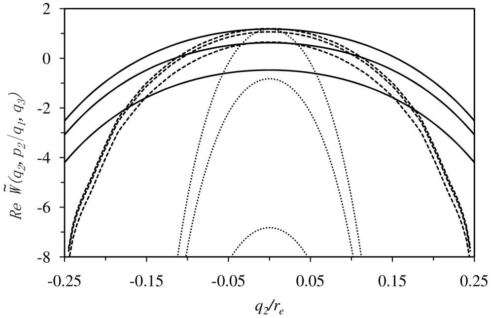
Figure 1: Real part of the combined total commutation function, $\tilde{W}=W-\beta{\cal H}$, for three particles, with $q_{1}=-q_{3}=-r_{\mathrm{e}}$ and $p_{1}=p_{3}=0$, at $\beta\hbar\omega=0.5$ (Lennard-Jones pair interaction, simple harmonic oscillator singlet potential, one dimension). The solid curves are the many-body expansion (pair), the dashed curves are the local state expansion (triplet),Attard20 and the dotted curves are the classical Maxwell-Boltzmann exponent, $-\beta{\cal H}({\bf q},{\bf p})$. From top to bottom in each series, the classical kinetic energy for the middle particle is $\beta p_{2}^{2}/2m=$ 0, 2, and 8. An arbitrary normalization constant has been added to each surface so that they coincide at $\{q_{2},p_{2}\}=\{0,0\}$.

Figure 1 shows the real part of the exponent for the phase space weight for three particles, $\mbox{Re }\tilde{W}^{(3)}(q_{1},p_{1};q_{2},p_{2};q_{3},p_{3})$, with the two exterior particles fixed at $\pm r_{\mathrm{e}}$ with zero momentum. Three approaches are compared: the present many-body expansion (pair level), a subsequently published local state expansion (triplet level; one variable and two fixed particles),Attard20 and the classical Maxwell-Boltzmann exponent. (The imaginary part of the exponent, which also contributes to the real part of the phase space weight, is not shown.) Overall, the data in Fig. 1 reveal that the two quantum approaches qualitatively agree in that there is substantial cancelation of the classical core repulsion between the Lennard-Jones particles. This means that the quantum particles will approach each other and interpenetrate much more deeply than their classical counterparts. The pair many-body expansion shows more cancelation than the triplet local state expansion. The two approaches also agree in predicting that higher values of momentum are more accessible in the quantum case than is classically predicted. However, for this, the real part of the exponent, the many-body expansion shows greater variation with momentum than does the local state expansion. Since the Monte Carlo simulation results for the average energy given by the local state expansion appear to be in good agreement with benchmark results for this system,Attard20 the quantitative disagreement between the present many-body expansion (pair level) and the subsequent local state expansion (triplet level)Attard20 does not bode well for the present approach.

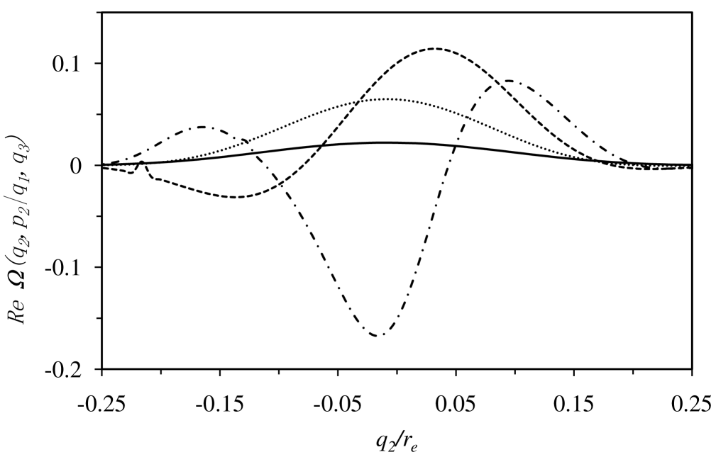
Figure 2: The real part of the phase space weight given by the many-body expansion (pair level) for three particles, with $q_{1}=-r_{\mathrm{e}}$, $p_{1}r_{\mathrm{e}}/\hbar=8.38$ ($\beta p_{1}^{2}/2m=5$), and $q_{3}=r_{\mathrm{e}}$, $p_{3}r_{\mathrm{e}}/\hbar=-11.85$ ($\beta p_{3}^{2}/2m=10$) at $\beta\hbar\omega=0.5$ (Lennard-Jones pair interaction, simple harmonic oscillator singlet potential, one dimension). The solid curve is $p_{2}r_{\mathrm{e}}/\hbar=0$, the dotted curve is $p_{2}r_{\mathrm{e}}/\hbar=5.24$, the dashed curve is $p_{2}r_{\mathrm{e}}/\hbar=10.5$, and the dash-dotted curve is $p_{2}r_{\mathrm{e}}/\hbar=18.7$.

Figure 2 shows the real part of the phase space weight, $\mbox{Re }\Omega^{(3)}({\bf q},{\bf p})=\mbox{Re }\exp\tilde{W}^{(3)}({\bf q},{\bf p})$, when the neighboring particles have non-zero momentum. The results seem unphysical. In particular, the increase in magnitude of the density with increase in momentum does not seem to be correct. It appears to be the source of an unrealistically high average kinetic energy when the pair many-body expansion commutation function is used in the Monte Carlo simulations (not shown). The dramatic oscillations with position and with momentum, and large negative values, also seem unphysical, particularly considering their relatively large magnitude. Although the local state expansion also gives region of phase space with negative weight,Attard20 the magnitude of the density in such regions is quite small relative to the maximum magnitude, and so for that approach they either cancel or contribute negligibly to any phase space average.

One can obtain a feeling for the limitations of the pair terminated many-body expansion by writing out the $N=3$ case explicitly. In this case Eq. (2.12), in which the singlet terms are absent, yields

$$\nabla\tilde{W}^{(3)}\cdot\nabla\tilde{W}^{(3)}$$ (C.3)

$$= \nabla_{1}\tilde{w}^{(2)}_{12}\!\cdot\!\nabla_{1}\tilde{w}^{(2)}_{12}+2\nabla_{1}\tilde{w}^{(2)}_{12}\!\cdot\!\nabla_{1}\tilde{w}^{(2)}_{13}+\nabla_{1}\tilde{w}^{(2)}_{13}\!\cdot\!\nabla_{1}\tilde{w}^{(2)}_{13}$$

$$\!+\nabla_{2}\tilde{w}^{(2)}_{21}\!\cdot\!\nabla_{2}\tilde{w}^{(2)}_{21}+2\nabla_{2}\tilde{w}^{(2)}_{21}\!\cdot\!\nabla_{2}\tilde{w}^{(2)}_{23}+\nabla_{2}\tilde{w}^{(2)}_{23}\!\cdot\!\nabla_{2}\tilde{w}^{(2)}_{23}$$

$$\!+\nabla_{3}\tilde{w}^{(2)}_{31}\!\cdot\!\nabla_{3}\tilde{w}^{(2)}_{31}+2\nabla_{3}\tilde{w}^{(2)}_{31}\!\cdot\!\nabla_{3}\tilde{w}^{(2)}_{32}+\nabla_{3}\tilde{w}^{(2)}_{32}\!\cdot\!\nabla_{3}\tilde{w}^{(2)}_{32}$$

$$\approx \nabla_{1}\tilde{w}^{(2)}_{12}\!\cdot\!\nabla_{1}\tilde{w}^{(2)}_{12}+\nabla_{2}\tilde{w}^{(2)}_{21}\!\cdot\!\nabla_{2}\tilde{w}^{(2)}_{21}+\nabla_{2}\tilde{w}^{(2)}_{23}\!\cdot\!\nabla_{2}\tilde{w}^{(2)}_{23}$$

$$\mbox{ }+\nabla_{3}\tilde{w}^{(2)}_{32}\!\cdot\!\nabla_{3}\tilde{w}^{(2)}_{32}+2\nabla_{2}\tilde{w}^{(2)}_{21}\!\cdot\!\nabla_{2}\tilde{w}^{(2)}_{23}.$$

The second approximation retains only the nearest neighbor contributions. One sees that the result in the text for the many-body expansion terminated at the pair level, Eq. (2.13), neglects the final term here. There is no reason to suppose that the neglected term is smaller in magnitude than those that are retained. (The commutation function is complex; the retained terms are not in general positive.)

One can conclude from this that for more than two particles, the many-body expansion of the total commutation function terminated at the pair level is inconsistent with its temperature derivative based on the above approximation to the non-linear term. It would mean, for example, that the commutation function at one temperature, $W^{(N)}({\bf q},{\bf p};\beta)$, formed using the series of singlet and pair commutation functions obtained by summing over energy states at that temperature, would not be equal to that obtained by integrating the total commutation function from a higher temperature, $W^{(N)}({\bf q},{\bf p};\beta_{0})$, using the approximation for the temperature derivative. Alternatively, the correct temperature derivative implies the existence of three-body terms, which contradicts the termination of the many-body expansion at the pair level. This inconsistency does not appear to be negligible, and is no doubt responsible for the unphysical results exhibited in the figures above.

This result, together with those in the figures and the unpublished simulations, suggest that the many-body expansion advocated in the text is not viable at the pair level, and perhaps not more generally. It appears that the local state expansionAttard20 represents the path forward for quantum statistical mechanics in classical phase space.

References

• (1) E. Wigner, “On the Quantum Correction for Thermodynamic Equilibrium”, Phys. Rev. 40, 749 (1932).
• (2) J. G. Kirkwood, “Quantum Statistics of Almost Classical Particles”, Phys. Rev. 44, 31 (1933).
• (3) P. Attard, Entropy Beyond the Second Law. Thermodynamics and Statistical Mechanics for Equilibrium, Non-Equilibrium, Classical, and Quantum Systems, (IOP Publishing, Bristol, 2018).
• (4) P. Attard, “Quantum Statistical Mechanics in Classical Phase Space. Expressions for the Multi-Particle Density, the Average Energy, and the Virial Pressure”, arXiv:1811.00730 [quant-ph] (2018).
• (5) P. Attard, “Quantum Statistical Mechanics in Classical Phase Space. Test Results for Quantum Harmonic Oscillators”, arXiv:1811.02032 (2018).
• (6) P. Attard, “Quantum Statistical Mechanics in Classical Phase Space. III. Mean Field Approximation Benchmarked for Interacting Lennard-Jones Particles”, arXiv:1812.03635 [quant-ph] (2018).
• (7) A. Hernando and J. Vaníček, “Imaginary-time nonuniform mesh method for solving the multidimensional Schrödinger equation: Fermionization and melting of quantum Lennard-Jones crystals”, Phys. Rev. A 88, 062107 (2013). arXiv:1304.8015v2 [quant-ph] (2013).
• (8) P. Attard, “Fermionic Phonons: Exact Analytic Results and Quantum Statistical Mechanics for a One Dimensional Harmonic Crystal”, arXiv:1903.06866 [quant-ph] (2019).
• (9) A. Messiah, Quantum Mechanics, (North-Holland, Amsterdam, Vols I and II, 1961).
• (10) In Ref. [Attard19, ] the symmetrization factor was shown correct for fermion statistics via a proof by induction that the number of even and odd permutations of $N$ objects were equal. A much simpler proof is as follows: Suppose that $\{\hat{\mathrm{P}}_{\alpha}\}_{\alpha=1}^{N!}$ is any set of permutation operators giving all the $N!$ permutations of $N$ objects. Let $\hat{\mathrm{P}}_{\alpha}^{\prime}=\hat{\mathrm{P}}_{jk}\hat{\mathrm{P}}_{\alpha}$, where $\hat{\mathrm{P}}_{jk}$ transposes objects $j$ and $k$. Clearly $\hat{\mathrm{P}}_{\alpha}^{\prime}$ has opposite parity to $\hat{\mathrm{P}}_{\alpha}$. Since $\{\hat{\mathrm{P}}_{\alpha}^{\prime}\}_{\alpha=1}^{N!}$ is also a set giving all the $N!$ permutations of $N$ objects, it follows that the number of even permutations of $N$ objects must equal the number of odd permutations.
• (11) R. K. Pathria, Statistical Mechanics, (Pergamon Press, Oxford, 1972).
• (12) J.-P. Hansen and I. R. McDonald Theory of Simple Liquids, (Academic Press, London, 1986).
• (13) P. Attard, Thermodynamics and Statistical Mechanics: Equilibrium by Entropy Maximisation (Academic Press, London, 2002).
• (14) T. Morita and K Hiroike, “A New Approach to the Theory of Classical Fluids. III —General Treatment of Classical Systems—”, Progr. Theor. Phys. 25, 537–578 (1961).
• (15) G. Stell, “Cluster Expansions for Classical Systems in Equilibrium”, in The Equilibrium Theory of Classical Fluids, (H. L. Frisch and J. L. Lebowitz, eds, p. II:171–266, W. A. Benjamin, New York, 1964).
• (16) P. Attard, “Pair Hypernetted Chain Closure for Fluids with Three-body Potentials. Results for Argon with the Axilrod-Teller Triple Dipole Potential.” Phys. Rev. A 45, 3659–3669 (1992).
• (17) E. Merzbacher, Quantum Mechanics, (Wiley, New York, 2nd ed., 1970).
• (18) P. Attard, “Quantum Statistical Mechanics in Classical Phase Space. V. Quantum Local, Average Global”, arXiv:2005.06165 [quant-ph] (2020).