Robust DCD-Based Recursive Adaptive Algorithms

Abstract

The dichotomous coordinate descent (DCD) algorithm has been successfully used for significant reduction in the complexity of recursive least squares (RLS) algorithms. In this work, we generalize the application of the DCD algorithm to RLS adaptive filtering in impulsive noise scenarios and derive a unified update formula. By employing different robust strategies against impulsive noise, we develop novel computationally efficient DCD-based robust recursive algorithms. Furthermore, to equip the proposed algorithms with the ability to track abrupt changes in unknown systems, a simple variable forgetting factor mechanism is also developed. Simulation results for channel identification scenarios in impulsive noise demonstrate the effectiveness of the proposed algorithms.

I Introduction

adaptive filtering has been a prominent technique in a variety of applications such as system identification, active noise control, and echo cancellation (EC) [1]. The least mean square (LMS) and recursive least squares (RLS) algorithms represent two typical families of adaptive algorithms [2],[3],[4],[5],[6],[7]. The complexity of LMS is $\mathcal{O}(M)$ arithmetic operations per sample (ops), where $M$ is the filter length, but its convergence is slow especially when the input signal is highly correlated. RLS improves the convergence at the cost of a high complexity of $\mathcal{O}(M^{2})$ ops. To reduce the complexity, some fast RLS algorithms were proposed as summarized in [1, Chapter 14]. However, these fast algorithms are numerically unstable in finite precision implementation since they are based on the matrix inversion.

Alternatively, the dichotomous coordinate descent (DCD) iterations for solving the normal equations in the RLS algorithms were proposed [8]. They result in not only numerically stable adaptive algorithms but also in performance comparable to that of the original RLS algorithm. An important property of the DCD algorithm is that it only requires addition and shift operations, which are simpler for implementation than multiplication and division, and thus it is well suited to real-time implementation. Moreover, the DCD-RLS algorithm reduces the complexity to $\mathcal{O}(M)$ ops for input signals with the tapped-delay structure. The DCD algorithm was also applied for the complexity reduction in the affine projection algorithm [9], sparse signal recovery [10], and distributed estimation [11].

Regrettably, the LMS and RLS algorithms undergo performance deterioration in impulsive noise [12], owing to the squared-error based minimization criteria. Realizations of impulsive noise process are sparse and random with amplitude far higher than the Gaussian noise, and therefore, best modeled by heavy-tailed distributions, e.g., the $\alpha$-stable distribution. Such noise scenarios are common in such as echo cancellation, underwater acoustics, audio processing, array processing, distributed processing and communications [13],[14],[15],[16],[17],[18],[19],[20]. For adapting impulsive noise scenarios, existing literature have reported various robust approaches [21],[22, 23]. For instance, the recursive least M-estimate (RLM) algorithm [24] exploits the Hampel’s M-estimate function to suppress impulsive interferences. Based on the $l_{p}$-norm of errors, the recursive least $p$-norm (RL$p$N) algorithm was developed [25]. By gathering all the $p$-norms from $p=1$ to 2 of the error, the continuous mixed $p$-norms (CMPN) algorithm was derived [26]; however, it has slow convergence for correlated inputs due to the gradient descent (GD) principle. Taking advantage of the Geman-McClure (GMC) estimator, a recursive algorithm [27] for Volterra system identification was derived, which shows a better performance than RL$p$N and RLM algorithms in impulsive noise modeled by the $\alpha$-stable distribution [13]. When impulsive noise appears, by incorporating the step-size scaler into the update term, a robust subband algorithm was developed [28]. The correntropy measures the similarity between two variables, which is helpful for suppressing large outliers; thus, the maximum correntropy criterion (MCC) has been used for improving the anti-jamming capability of adaptive filters to impulsive noise, yielding the GD-based MCC [29, 30, 31] and recursive MCC (RMCC) algorithms [32, 33]. However, these robust recursive algorithms have also high complexity of $\mathcal{O}(M^{2})$ ops. In particular, the complexity of the fixed-point variant of MCC algorithm in [32] is $\mathcal{O}(M^{3})$ due to the direct inverse of an $M\times M$ matrix.

This work focuses on a class of low-complexity robust algorithms against impulsive noise by resorting to the DCD approach. Concretely, a generalized DCD-based robust recursion is derived. By applying different robust strategies to this recursion, we develop DCD-based robust algorithms, such as the DCD-RMCC, DCD-RLM, and DCD-RL$p$N algorithms. We also design a variable forgetting factor (VFF) scheme for improving the tracking capability of the algorithms.

II DCD-Based Robust Algorithms

II-A Unified Formulation

Suppose that at time instant $n$, the desired signal $d_{n}$ and an $M\times 1$ input signal vector $\bm{x}_{n}$ are available and obey the relation $d_{n}=\bm{x}_{n}^{\text{T}}\bm{w}^{o}+v_{n}$, where the $M\times 1$ vector $\bm{w}^{o}$ needs to be estimated, and $(\cdot)^{\text{T}}$ denotes the transpose. The additive noise with impulsive behavior, $v_{n}$, here is described by the $\alpha$-stable process, also called the $\alpha$-stable noise. A (symmetric) $\alpha$-stable random variable is usually characterized by the characteristic function [13]

$$\phi(t)=\exp(-\gamma\lvert t\lvert^{\alpha}).$$ (1)

The characteristic exponent $\alpha\in(0,2]$ describes the impulsiveness of the noise (smaller $\alpha$ leads to more outliers) and $\gamma>0$ represents the dispersion degree of the noise. Note that when $\alpha$ = 1 and 2, it reduces to the Cauchy and Gaussian distributions, respectively.

To effectively estimate $\bm{w}^{o}$ in such noise scenarios, we define a unified robust exponentially weighted least squares problem:

$$\bm{w}_{n}=\arg\min\limits_{\bm{w}}\left\{\sum\limits_{i=0}^{n}\lambda^{n-i}\varphi\left(d_{i}-\bm{x}_{i}^{\text{T}}\bm{w}\right)+\delta_{n}\lVert\bm{w}\rVert_{2}^{2}\right\},$$ (2)

where $0\ll\lambda<1$ is the forgetting factor, $\delta_{n}>0$ is a regularization parameter, and $\varphi(\cdot)$ is a function that specifies the robustness against impulsive noise.

By setting the derivative of (2) with respect to $\bm{w}$ to zero, we arrive at the normal equations:

$$\bm{R}_{n}\bm{w}_{n}=\bm{z}_{n},$$ (3)

where

$$\begin{array}[]{rcl}\begin{aligned} \bm{R}_{n}&=\sum\limits_{i=0}^{n}\lambda^{n-i}f_{i}\bm{x}_{i}\bm{x}_{i}^{\text{T}}+\delta_{n}\bm{I}_{M}\\ &=\lambda\bm{R}_{n-1}+f_{n}\bm{x}_{n}\bm{x}_{n}^{\text{T}}+(\delta_{n}-\lambda\delta_{n-1})\bm{I}_{M}\end{aligned}\end{array}$$ (4)

is the time-averaged autocorrelation matrix of $\bm{x}_{n}$,

$$\begin{array}[]{rcl}\begin{aligned} \bm{z}_{n}&=\sum\limits_{i=0}^{n}\lambda^{n-i}f_{i}d_{i}\bm{x}_{i}\\ &=\lambda\bm{z}_{n-1}+f_{n}d_{n}\bm{x}_{n}\end{aligned}\end{array}$$ (5)

is the time-averaged crosscorrelation vector of $d_{n}$ and $\bm{x}_{n}$, and $\bm{I}_{M}$ is an $M\times M$ identity matrix. Also, $f_{n}=\varphi^{\prime}(\epsilon_{n})/\epsilon_{n}$, where $\epsilon_{n}=d_{n}-\bm{x}_{n}^{\text{T}}\bm{w}_{n}$ is the a posteriori error and $\varphi^{\prime}(\epsilon_{n})$ is the derivative of $\varphi(\epsilon_{n})$.

At time instant $n-1$, let $\hat{\bm{w}}_{n-1}$ denote the approximate solution of (3) for estimating $\bm{w}^{o}$, and the corresponding residual vector is $\bm{r}_{n-1}=\bm{z}_{n-1}-\bm{R}_{n-1}\hat{\bm{w}}_{n-1}$. By defining $\Delta\bm{w}_{n}=\bm{w}_{n}-\hat{\bm{w}}_{n-1}$, from (3) we obtain an auxiliary system of equations:

$$\begin{array}[]{rcl}\begin{aligned} \bm{R}_{n}\Delta\bm{w}_{n}=\bm{z}_{n}-\bm{R}_{n}\hat{\bm{w}}_{n-1}\triangleq\bm{b}_{n}.\end{aligned}\end{array}$$ (6)

Applying the recursive expressions (4) and (5), $\bm{b}_{n}$ can be rewritten as

$$\bm{b}_{n}=\lambda\bm{r}_{n-1}+f_{n}e_{n}\bm{x}_{n}-(\delta_{n}-\lambda\delta_{n-1})\hat{\bm{w}}_{n-1},$$ (7)

where $e_{n}=d_{n}-\bm{x}_{n}^{\text{T}}\hat{\bm{w}}_{n-1}$ denotes the a priori error.

By using the DCD algorithm to solve the problem in (6), we arrive at an approximate solution of the original normal equations (3):

$$\hat{\bm{w}}_{n}=\hat{\bm{w}}_{n-1}+\Delta\hat{\bm{w}}_{n}.$$ (8)

Although (7) shows that $\bm{b}_{n}$ requires the residual error vector of the original system (3), after some algebra we notice that it is equivalent to the residual error vector for the auxiliary system (6), i.e., $\bm{r}_{n}=\bm{z}_{n}-\bm{R}_{n}\hat{\bm{w}}_{n}=\bm{b}_{n}-\bm{R}_{n}\Delta\hat{\bm{w}}_{n}$. At time index $n$, $f_{n}$ in (7) is not yet available, but by resorting to the a priori error, we may approximate $f_{n}$ as

$$f_{n}\approx\varphi^{\prime}(e_{n})/e_{n}.$$ (9)

TABLE I: DCD-Based Robust Recursive Update

Parameters: $0\ll\lambda<1,\;\delta_{0}>0$

Initialization: $\bm{R}_{0}=\delta_{0}\bm{I}_{M},\;\hat{\bm{w}}_{0}=\bm{0},\;\bm{r}_{0}=\bm{0}$

for $n=1,...$

$e_{n}=d_{n}-\bm{x}_{n}^{\text{T}}\hat{\bm{w}}_{n-1}$

$\bm{R}_{n}=\lambda\bm{R}_{n-1}+f_{n}\bm{x}_{n}\bm{x}_{n}^{T}+(\delta_{n}-\lambda\delta_{n-1})\bm{I}_{M}$

$\bm{b}_{n}=\lambda\bm{r}_{n-1}+f_{n}e_{n}\bm{x}_{n}-(\delta_{n}-\lambda\delta_{n-1})\hat{\bm{w}}_{n-1}$

Using DCD iterations to solve $\bm{R}_{n}\Delta\bm{w}_{n}=\bm{b}_{n}$, which yields $\Delta\hat{\bm{w}}_{n}$ and $\bm{r}_{n}$

$\hat{\bm{w}}_{n}=\hat{\bm{w}}_{n-1}+\Delta\hat{\bm{w}}_{n}$

end

This completes the derivation of DCD-based robust recursion, summarized in Table I.

Table II presents the leading DCD algorithm for solving the system of equations $\bm{R}_{n}\Delta\bm{w}_{n}=\bm{b}_{n}$ (readers can refer to [9, 8] for details), where $[\bm{r}_{n}]_{l}$ is the $l$-th entry of $\bm{r}_{n}$, and $[\bm{R}_{n}]_{l,l}$ and $[\bm{R}_{n}]_{:,l}$ are the $(l,l)$-th entry and the $l$-th column of $\bm{R}_{n}$, respectively. Herein, $[-H,H]$ denotes the amplitude range for elements of the solution vector $\Delta\hat{\bm{w}}_{n}$. It is often chosen as a power-of-two number so that all multiplications by $\mu$ can be implemented by bit-shifts. $M_{b}$ is the number of bits for a fixed-point representation of $\hat{\bm{w}}_{n}$ within the range $[-H,H]$. $N_{u}$ stands for a maximum number of elements in $\Delta\hat{\bm{w}}_{n}$ that are updated. The solution $\Delta\hat{\bm{w}}_{n}$ approaches the optimal one (i.e., $\Delta\hat{\bm{w}}_{n}=\bm{R}_{n}^{-1}\bm{b}_{n}$ ) as $N_{u}$ increases. As seen in Table II, the implementation of DCD only requires shift and addition operations, excluding multiplication and division operations.

TABLE II: Leading DCD Algorithm

Parameters: $H,\;N_{u},\;M_{b}$,

Initialization: $\Delta\hat{\bm{w}}_{n}=\bm{0},\;\bm{r}_{n}=\bm{b}_{n},\;y=1,\;\mu=H/2$

for $j=1,...,N_{u}$

$l=\arg\max\limits_{j=1,...,M}\{\rvert[\bm{r}_{n}]_{j}\rvert\}$

while $\rvert[\bm{r}_{n}]_{l}\rvert\leq(\mu/2)[\bm{R}_{n}]_{l,l}$ and $y\leq M_{b}$

$y=y+1$, $\mu=\mu/2$

end

if $y>M_{b}$

break

else

$[\Delta\hat{\bm{w}}_{n}]_{l}\leftarrow[\Delta\hat{\bm{w}}_{n}]_{l}+\mu\text{sign}([\bm{r}_{n}]_{l})$

$\bm{r}_{n}\leftarrow\bm{r}_{n}-\mu\text{sign}([\bm{r}_{n}]_{l})[\bm{R}_{n}]_{:,l}$

end

end

II-B Robust Strategies

TABLE III: Some Robust DCD-based Algorithms

Robust Algorithms	$\varphi(e)$ in (2)	$f(e)=\varphi^{\prime}(e)/e$ in (9)
DCD-RMCC	$\frac{1}{\sqrt{2\pi}\beta}\left[1-\exp\left(-\frac{e^{2}}{2\beta^{2}}\right)\right]$	$\exp\left(-\frac{e^{2}}{2\beta^{2}}\right)$
DCD-RLM	$\left\{\begin{aligned} &e^{2}/2,\text{ if }|e|\leq\xi\\ &\xi^{2}/2,|e|>\xi,\end{aligned}\right.$	$\left\{\begin{aligned} &1,\text{ if }|e|\leq\xi\\ &0,|e|>\xi,\end{aligned}\right.$
DCD-RL$p$N	$|e|^{p}$	$|e|^{p}/(|e|^{2}+\varepsilon)$

Applying a particular robust strategy to define $\varphi(e)$ in (2), we can compute $f_{n}$ by (9) to arrive at a DCD-based robust algorithm. Table III gives examples of $\varphi(e)$ for the DCD-RMCC, DCD-RLM, and DCD-RL$p$N algorithms derived from the widely studied MCC, M-estimate, and $l_{p}$-norm strategies, respectively. We note the following about the proposed algorithms:

1) For the DCD-RMCC algorithm, $\beta>0$ denotes the kernel width. When $\beta\rightarrow\infty$, $f_{n}$ approaches 1 so that the DCD-RMCC algorithm reduces to the DCD-RLS algorithm. When $\beta\rightarrow 0$, $f_{n}$ becomes 0, and the DCD-RMCC update is frozen. Thus, $\beta$ balances the robustness and dynamic performance of the algorithm in impulsive noise.

2) The DCD-RLM algorithm uses the modified Huber M-estimate function [35] for $\varphi(e)$. When $|e_{n}|<\xi$, thus $f_{n}$ equals 1 so that the DCD-RLM algorithm becomes the DCD-RLS algorithm. Otherwise, $f_{n}$ becomes 0 to stop the update (ideally, this only happens when the impulsive noise appears). To effectively suppress the impulsive noise, the threshold $\xi$ is adaptively adjusted by $\xi=\tau\hat{\sigma}_{e,n}$,

$$\hat{\sigma}_{e,n}^{2}=\zeta\hat{\sigma}_{e,n-1}^{2}+c_{\sigma}(1-\zeta)\text{med}(\bm{a}_{n}^{e}),$$ (10)

where $\left.0<\zeta<1\right.$ is a weighting factor (except $\zeta=0$ at the algorithm start), $\text{med}(\cdot)$ is the median operator which helps to remove outliers in the data window $\bm{a}_{n}^{e}=[e_{n}^{2},e_{n-1}^{2},...,e_{n-N_{w}+1}^{2}]$, and $c_{\sigma}=1.483(1+5/(N_{w}-1))$ is the correction factor [24]. It is worth noting that, the window length $N_{w}$ should be properly chosen. Larger $N_{w}$ makes a more robust estimate $\hat{\sigma}_{e,n}^{2}$ from (10) but requires a higher complexity. A typical value of $\tau$ is 2.576. If $e_{n}$ is assumed to be Gaussian (which is reasonable except when being polluted by impulsive noise), this value means the 99% confidence to prevent $e_{n}$ from contributing to the update for $|e_{n}|\geq\xi$ [24].

3) The convergence of the RL$p$N algorithm in the $\alpha$-stable noise requires $0<p<\alpha$. If $p=2$, the DCD-RL$p$N algorithm will also become the DCD-RLS algorithm. When $p=1$, this corresponds to the recursion sign algorithm [37] with good robustness against impulsive noise.

Remark 1: In a nutshell, when impulsive noise happens, its negative influence on the updates of $\bm{R}_{n}$ and $\bm{b}_{n}$ will be lowered significantly due to by multiplying a tiny scaler $f_{n}$ into the updates. Then, we can generalize the DCD recursion to find $\Delta\bm{\hat{}}{w}_{n}$ from the system of equations $\bm{R}_{n}\Delta\bm{w}_{n}=\bm{b}_{n}$ with impulse-free. Hence, according to (8), the proposed DCD-based algorithms can work well in impulsive noise.

II-C Computational Complexity

The direct solution of (3) is $\bm{w}_{n}=\bm{R}_{n}^{-1}\bm{z}_{n}$. The regularization $\delta_{n}$ is to maintain the numerical stability of this solution [1]. However, this leads to the complexity of $\mathcal{O}(M^{3})$ due to the matrix inversion $\bm{R}_{n}^{-1}$. Generally, $\delta_{n}$ is chosen as $\delta_{n}=\lambda^{n+1}\delta_{0}$ (e.g., in this paper), it makes (4) become $\bm{R}_{n}=\lambda\bm{R}_{n-1}+f_{n}\bm{x}_{n}\bm{x}_{n}^{\text{T}}$. Then, using the matrix inversion lemma, $\bm{R}_{n}^{-1}$ can be calculated in a recursive way so that the complexity of the resulting algorithm is $\mathcal{O}(M^{2})$, while it is still high for large $M$.

TABLE IV: Complexity of Algorithms per Input Sample

Algorithms	Additions	Multiplications	Divisions
LMS	$2M$	$2M+1$	0
(R) RLS	$3M^{2}+M$	$4M^{2}+4M+1$	1
(R) DCD RLS (general input)	$M^{2}+2M+P_{a}$	$\frac{3}{2}M^{2}+\frac{7}{2}M+1$	0
(R) DCD RLS (tap-delayed input)	$3M+P_{a}$	$5M+2$	0

Table IV mainly compares the complexity of robust (R) RLS-type with that of proposed (R) DCD variant in terms of ops, where we drop the calculation of $f_{n}$ dependent on a specific robust strategy. As in [8], the DCD recursion requires $P_{a}=2N_{u}M+M_{b}$ additions at most for finding $\Delta\hat{\bm{w}}_{n}$. Thus, it is clear to see from Table IV, for general input vector form, the DCD version reduces the complexity by at least a factor of 0.5 in contrast with the original algorithm, in terms of multiplications and additions. On the other hand, if the input vector $\bm{x}_{n}$ has a tapped-delay structure, i.e., $\bm{x}_{n}=[x_{n},x_{n-1},...,x_{n-M+1}]^{\text{T}}$, where $x_{n}$ is a data sample at time $n$, the calculation of $\bm{R}_{n}$ will be simplified. Specifically, assuming $f_{n}\approx f_{n-1}$, we can obtain the lower-right $(M-1)\times(M-1)$ block of $\bm{R}_{n}$ by copying the upper-left $(M-1)\times(M-1)$ block of $\bm{R}_{n-1}$. Then, considering the symmetry of $\bm{R}_{n}$, we only need the calculation of its first column:

$$\begin{array}[]{rcl}[\bm{R}_{n}]_{:,1}\approx\lambda[\bm{R}_{n-1}]_{:,1}+f_{n}x_{n}\bm{x}_{n}.\end{array}$$ (11)

Equation (11) is exact when $f_{n}=1$ [8]. As claimed in Section II. B, $f_{n}$ is normally close to 1, and becomes very small to suppress the update only when the impulsive noise happens. As such, using (11) is also suitable for computing $\bm{R}_{n}$ in the proposed DCD recursion. In this scenario, the complexity is reduced to the same order of magnitude as that of LMS. This reduction is considerable especially for a long $\bm{w}^{o}$ such as in EC applications.

II-D Improving Tracking Performance

For the proposed algorithms, there is also a trade-off between steady-state error and tracking capability for abrupt changes of $\bm{w}^{o}$, because of using the fixed forgetting factor $\lambda$. To address this problem, one may utilize the adaptive combination (AC) of two independently running DCD-based filters. Like the AC-RL$p$N algorithm in [25], it combines RL$p$N filters with the large forgetting factor for low steady-state error and with the small one for good tracking capability. However, it requires at least double complexity of the original algorithm. Alternatively, the VFF has been also an effective mechanism for improving the original RLS algorithm [38, 39, 40]. Consequently, to equip the proposed DCD-based algorithms, we also propose a simple VFF scheme:

$$\begin{array}[]{rcl}\lambda_{n}=\lambda_{\text{min}}+(1-\lambda_{\text{min}})\exp(-\rho e_{n,f}^{2}),\end{array}$$ (12)

where $\rho>0$ is a design parameter, $e_{n,f}^{2}$ is the impulse-free squared error which can be estimated by (10). As $n\rightarrow\infty$, $e_{n,f}^{2}$ converges to a small value, and according to (12), $\lambda_{n}$ approaches 1, thus reducing the steady-state error. When $\bm{w}^{o}$ has a sudden change, $e_{n,f}^{2}$ becomes large due the mismatch estimation at that time, and $\lambda_{n}$ will approach a small forgetting factor $\lambda_{\text{min}}$, thus speeding up the convergence.

III Simulation results

In this section, simulations are conducted for identifying the network echo channel response $\bm{w}^{o}$ of length $M$ using an adaptive filter. The echo channels in Fig. 1 are from the ITU-T G.168 standard, with $M=128$ taps [41]. For the tapped-delay input vector $\bm{x}_{n}$, its element $x_{n}$ is given by the first-order autoregressive model $x_{n}=\varrho x_{n-1}+\vartheta_{n}$, where $\vartheta_{n}$ is a zero-mean white Gaussian random process with unit variance. Both $\varrho=0$ (which is used only in Fig. 2(b)) and $\varrho=0.9$ correspond to the white and correlated inputs, respectively, with the eigenvalue spreads of 1 and 346. The $\alpha$-stable noise is set to $\alpha=1.4$ and $\gamma=1/20$. We use the normalized mean square deviation, $\text{NMSD}(n)=10\log_{10}(||\bm{w}_{n}-\bm{w}^{o}||_{2}^{2}/||\bm{w}^{o}||_{2}^{2})$, as a performance measure. All simulated curves are the average over 100 independent runs.

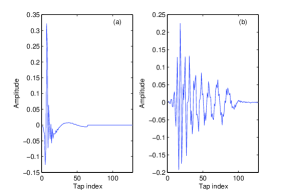
Figure 1: Network echo channels: (a) sparse channel, (b) disperse channel.

Fig. 2 shows the NMSD performance of the DCD-RLS, GD-based MCC, RMCC, and proposed DCD-RMCC algorithms. As expected for impulsive noise scenarios, the performance of the original DCD-RLS algorithm is poor, while the MCC-based algorithms are performing very well. The DCD-RMCC performance approaches that of the original RMCC algorithm as $N_{u}$ increases. In particular, $N_{u}=8\ll M$ (at most eight entries of $\bm{w}_{n}$ are updated per time $n$) has been enough for the DCD-RMCC performance to approach closely the RMCC performance regardless of whether $\bm{w}^{o}$ is sparse or not. However, as seen from Table IV, the DCD-RMCC with $N_{u}=8$ reduces significantly the complexity of the RMCC. Although the DCD-RMCC requires 2.5 times multiplications of the GD-based MCC, the former (even if with $N_{u}=1$) has much faster convergence than the latter. Likewise, the convergence of the proposed low-cost DCD-RLM and DCD-RL$p$N versions also approximate well that of the RLM and RL$p$N algorithms, respectively; these results are omitted for brevity.

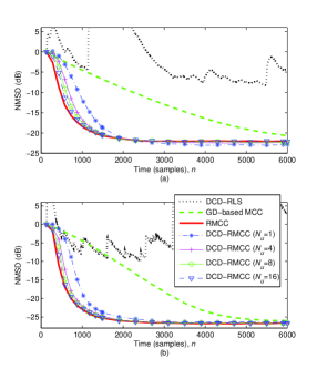
Figure 2: NMSD curves of the DCD-RLS and MCC-based algorithms: (a) sparse channel and correlated input; (b) disperse channel and white input. Parameters of algorithms are chosen as: $\lambda=0.998$ (all the algorithms); $\mu=0.001,\;\beta^{2}=0.6$ (GD-based MCC); $\beta^{2}=0.03$ (RMCC); $H=1,\;M_{b}=16$ (DCD).

Fig. 3 shows the NMSD of the proposed DCD-RMCC, DCD-RLM and DCD-RL$p$N algorithms, with $N_{u}=8$. The proposed algorithms show robustness in $\alpha$-stable noise and can arrive at similar performance by properly setting their parameters. This reason is they generally behave like the DCD-RLS and use a tiny $f_{n}$ to suppress the algorithms’ adaptation once the impulsive noise appears. In addition, we also show the DCD-CMPN algorithm by applying the CMPN criteria in [26], i.e., $\varphi(e)=\int_{1}^{2}|e|^{p}dp$ and $f(e)=\left((2|e|-1)\ln(|e|)-|e|+1\right)/\left(|e|\ln^{2}(|e|)\right)$. For the $l_{p}$-norm based algorithms, $p$ should be slightly less than $\alpha$ in $\alpha$-stable noise; thus, the DCD-RL$p$N may outperform the DCD-CMPN, since the latter inherits the behavior of $p>\alpha$.

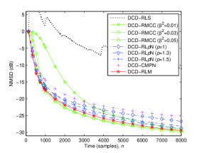
Figure 3: NMSD curves of DCD-based RLS algorithms for the sparse channel. Parameters setting of algorithms is: $\lambda=0.9998$ (all the recursive algorithms); $\zeta=0.99,\;N_{w}=9$ (DCD-RLM). [$N_{u}=8$].

Fig. 4 demonstrates the tracking capability of the proposed algorithms, in a scenario where the echo channel changes at time $n=8001$ by shifting its impulse response by 12 samples. As one can see, using the proposed VFF instead of the fixed one, the DCD-based algorithms can reduce the steady-state error and improve the tracking capability.

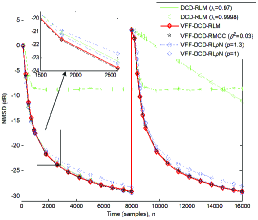
Figure 4: NMSD curves of DCD-based RLS algorithms for the sparse channel. Parameters of VFF are: $\zeta=0.99,\;N_{w}=9,\;\rho=3,\;\lambda_{\text{min}}=0.97$.

IV Conclusion

We have proposed a general low-complexity recursion for developing RLS-type adaptive filtering algorithms operating in impulsive noise scenarios. This is based on using DCD iterations. As examples of the MCC, M-estimator, and $p$-norm strategies applied to this recursion, we have developed the DCD-RMCC, DCD-RLM, and DCD-RL$p$N algorithms, respectively. These algorithms show a performance similar to that of their high-complexity counterparts, RMCC, RLM, and RLpN algorithms, respectively. To improve the tracking capability of the algorithms, a simple time-varying forgetting factor mechanism has also been developed. Simulation results demonstrate the performance of the proposed algorithms.

References

- [1] A. H. Sayed, Fundamentals of adaptive filtering. John Wiley & Sons, 2003.
- [2] R. C. de Lamare and R. Sampaio-Neto, “Adaptive reduced-rank mmse filtering with interpolated fir filters and adaptive interpolators,” IEEE Signal Processing Letters, vol. 12, no. 3, pp. 177–180, March 2005.
- [3] R. C. de Lamare and R. Sampaio-Neto, “Reduced-rank adaptive filtering based on joint iterative optimization of adaptive filters,” IEEE Signal Processing Letters, vol. 14, no. 12, pp. 980–983, Dec 2007.
- [4] R. C. de Lamare and P. S. R. Diniz, “Set-membership adaptive algorithms based on time-varying error bounds for cdma interference suppression,” IEEE Transactions on Vehicular Technology, vol. 58, no. 2, pp. 644–654, Feb 2009.
- [5] R. C. de Lamare and R. Sampaio-Neto, “Adaptive reduced-rank processing based on joint and iterative interpolation, decimation, and filtering,” IEEE Transactions on Signal Processing, vol. 57, no. 7, pp. 2503–2514, July 2009.
- [6] R. C. de Lamare and R. Sampaio-Neto, “Reduced-rank space-time adaptive interference suppression with joint iterative least squares algorithms for spread-spectrum systems,” IEEE Transactions on Vehicular Technology, vol. 59, no. 3, pp. 1217–1228, March 2010.
- [7] R. C. de Lamare and R. Sampaio-Neto, “Sparsity-aware adaptive algorithms based on alternating optimization and shrinkage,” IEEE Signal Processing Letters, vol. 21, no. 2, pp. 225–229, Feb 2014.
- [8] Y. V. Zakharov, G. P. White, and J. Liu, “Low-complexity RLS algorithms using dichotomous coordinate descent iterations,” IEEE Transactions on Signal Processing, vol. 56, no. 7, pp. 3150–3161, 2008.
- [9] Y. V. Zakharov, “Low-complexity implementation of the affine projection algorithm,” IEEE Signal Processing Letters, vol. 15, pp. 557–560, 2008.
- [10] Y. V. Zakharov, V. H. Nascimento, R. C. De Lamare, and F. G. D. A. Neto, “Low-complexity DCD-based sparse recovery algorithms,” IEEE Access, vol. 5, pp. 12 737–12 750, 2017.
- [11] Y. Yu, H. Zhao, R. C. de Lamare, Y. V. Zakharov, and L. Lu, “Robust distributed diffusion recursive least squares algorithms with side information for adaptive networks,” IEEE Transactions on Signal Processing, vol. 67, no. 6, pp. 1566–1581, 2019.
- [12] S. Zhang and J. Zhang, “Enhancing the tracking capability of recursive least p-norm algorithm via adaptive gain factor,” Digital Signal Processing, vol. 30, pp. 67 – 73, 2014.
- [13] C. L. Nikias and M. Shao, Signal processing with alpha-stable distributions and applications. Wiley-Interscience, 1995.
- [14] M. Zimmermann and K. Dostert, “Analysis and modeling of impulsive noise in broad-band powerline communications,” IEEE transactions on Electromagnetic compatibility, vol. 44, no. 1, pp. 249–258, 2002.
- [15] R. Fa, R. C. de Lamare, and L. Wang, “Reduced-rank stap schemes for airborne radar based on switched joint interpolation, decimation and filtering algorithm,” IEEE Transactions on Signal Processing, vol. 58, no. 8, pp. 4182–4194, Aug 2010.
- [16] M. Yukawa, R. C. de Lamare, and R. Sampaio-Neto, “Efficient acoustic echo cancellation with reduced-rank adaptive filtering based on selective decimation and adaptive interpolation,” IEEE Transactions on Audio, Speech, and Language Processing, vol. 16, no. 4, pp. 696–710, May 2008.
- [17] L. Wang, R. C. de Lamare, and M. Yukawa, “Adaptive reduced-rank constrained constant modulus algorithms based on joint iterative optimization of filters for beamforming,” IEEE Transactions on Signal Processing, vol. 58, no. 6, pp. 2983–2997, June 2010.
- [18] S. Xu, R. C. de Lamare, and H. V. Poor, “Distributed compressed estimation based on compressive sensing,” IEEE Signal Processing Letters, vol. 22, no. 9, pp. 1311–1315, Sep. 2015.
- [19] S. Xu, R. C. de Lamare, and H. V. Poor, “Adaptive link selection algorithms for distributed estimation,” Eurasip Journal on Advances in Signal Processing, no. 86, pp. 1–22, 2015.
- [20] T. G. Miller, S. Xu, R. C. de Lamare, and H. V. Poor, “Distributed spectrum estimation based on alternating mixed discrete-continuous adaptation,” IEEE Signal Processing Letters, vol. 23, no. 4, pp. 551–555, April 2016.
- [21] L. Landau, R. C. de Lamare, and M. Haardt, “Robust adaptive beamforming algorithms using the constrained constant modulus criterion,” IET Signal Processing, vol. 8, no. 5, pp. 447–457, July 2014.
- [22] H. Ruan and R. C. de Lamare, “Robust adaptive beamforming using a low-complexity shrinkage-based mismatch estimation algorithm,” IEEE Signal Processing Letters, vol. 21, no. 1, pp. 60–64, Jan 2014.
- [23] H. Ruan and R. C. de Lamare, “Robust adaptive beamforming based on low-rank and cross-correlation techniques,” IEEE Transactions on Signal Processing, vol. 64, no. 15, pp. 3919–3932, Aug 2016.
- [24] Y. Zou, S. Chan, and T. Ng, “Robust M-estimate adaptive filtering,” IEE Proceedings-Vision, Image and Signal Processing, vol. 148, no. 4, pp. 289–294, 2001.
- [25] Á. Navia-Vazquez and J. Arenas-Garcia, “Combination of recursive least -norm algorithms for robust adaptive filtering in alpha-stable noise,” IEEE Transactions on Signal Processing, vol. 60, no. 3, pp. 1478–1482, 2012.
- [26] H. Zayyani, “Continuous mixed -norm adaptive algorithm for system identification,” IEEE Signal Processing Letters, vol. 21, no. 9, pp. 1108–1110, 2014.
- [27] L. Lu, W. Wang, X. Yang, W. Wu, and G. Zhu, “Recursive Geman-mcclure estimator for implementing second-order Volterra filter,” IEEE Transactions on Circuits and Systems II: Express Briefs, vol. 66, no. 7, pp. 1272–1276, 2019.
- [28] J. Hur, I. Song, and P. Park, “A variable step-size normalized subband adaptive filter with a step-size scaler against impulsive measurement noise,” IEEE Transactions on Circuits and Systems II: Express Briefs, vol. 64, no. 7, pp. 842–846, 2016.
- [29] B. Chen, L. Xing, H. Zhao, N. Zheng, and J. C. Príncipe, “Generalized correntropy for robust adaptive filtering,” IEEE Transactions on Signal Processing, vol. 64, no. 13, pp. 3376–3387, 2016.
- [30] L. Shi, H. Zhao, and Y. Zakharov, “An improved variable kernel width for maximum correntropy criterion algorithm,” IEEE Transactions on Circuits and Systems II: Express Briefs, 2018.
- [31] B. Chen, L. Xing, J. Liang, N. Zheng, and J. C. Principe, “Steady-state mean-square error analysis for adaptive filtering under the maximum correntropy criterion,” IEEE signal processing letters, vol. 21, no. 7, pp. 880–884, 2014.
- [32] B. Chen, J. Wang, H. Zhao, N. Zheng, and J. C. Príncipe, “Convergence of a fixed-point algorithm under maximum correntropy criterion,” IEEE Signal Processing Letters, vol. 22, no. 10, pp. 1723–1727, 2015.
- [33] H. Radmanesh and M. Hajiabadi, “Recursive maximum correntropy learning algorithm with adaptive kernel size,” IEEE Transactions on Circuits and Systems II: Express Briefs, vol. 65, no. 7, pp. 958–962, 2018.
- [34] S. A. Kassam, Signal detection in non-Gaussian noise. Springer Science & Business Media, 2012.
- [35] S.-C. Chan and Y.-X. Zou, “A recursive least M-estimate algorithm for robust adaptive filtering in impulsive noise: fast algorithm and convergence performance analysis,” IEEE Transactions on Signal Processing, vol. 52, no. 4, pp. 975–991, 2004.
- [36] P. Petrus, “Robust Huber adaptive filter,” IEEE Transactions on Signal Processing, vol. 47, no. 4, pp. 1129–1133, 1999.
- [37] V. Mathews and S. Cho, “Improved convergence analysis of stochastic gradient adaptive filters using the sign algorithm,” IEEE Transactions on Acoustics, Speech, and Signal Processing, vol. 35, no. 4, pp. 450–454, 1987.
- [38] D.-J. Park, B.-E. Jun, and J.-H. Kim, “Fast tracking RLS algorithm using novel variable forgetting factor with unity zone,” Electronics Letters, vol. 27, no. 23, pp. 2150–2151, 1991.
- [39] C. Paleologu, J. Benesty, and S. Ciochina, “A robust variable forgetting factor recursive least-squares algorithm for system identification,” IEEE Signal Processing Letters, vol. 15, pp. 597–600, 2008.
- [40] Y. Cai, R. C. de Lamare, M. Zhao, and J. Zhong, “Low-complexity variable forgetting factor mechanism for blind adaptive constrained constant modulus algorithms,” IEEE Transactions on Signal Processing, vol. 60, no. 8, pp. 3988–4002, 2012.
- [41] Digital Network Echo Cancellers Recommendation, Std. ITU-TG.168 (V8), 2015.