figure \cftpagenumbersofftable
Artificial neural network to estimate the refractive index of a liquid infiltrating a chiral sculptured thin film
Patrick D. McAtee,a,∗ Satish T.S. Bukkapatnam,b and Akhlesh Lakhtakiaa
aThe Pennsylvania State University, Department of Engineering Science and Mechanics, University Park, PA 16802, USA
bTexas A&M University, Department of Industrial and Systems Engineering, College Station, TX 77843, USA
Abstract
We theoretically expanded the capabilities of optical sensing based on surface plasmon resonance in a prism-coupled configuration by incorporating artificial neural networks (ANNs). We used calculations modeling the situation in which an index-matched substrate with a metal thin film and a porous chiral sculptured thin film (CSTF) deposited successively on it is affixed to the base of a triangular prism. When a fluid is brought in contact with the exposed face of the CSTF, the latter is infiltrated. As a result of infiltration, the traversal of light entering one slanted face of the prism and exiting the other slanted face of the prism is affected. We trained two ANNs with differing structures using reflectance data generated from simulations to predict the refractive index of the infiltrant fluid. The best predictions were a result of training the ANN with simpler structure. With realistic simulated-noise, the performance of this ANN is robust.
1 Introduction
The ability to accurately detect small concentrations of chemicals and biochemicals, whether toxic or benign, is highly prized in chemical, pharmaceutical, medical, environmental, and food industries [1, 2]. Introduction of pathogens and toxins into the human body can arise from intentional contamination of essential infrastructure [3] as well as from unforeseen consequences of their otherwise necessary applications [4]. Even chemicals traditionally thought of as non-toxic in their bulk form, such as gold, could have harmful effects when ingested as nanoparticles [5, 6, 7]. Also, the concentrations of various chemicals in solutions and dispersions need to be determined in research as well as industrial laboratories [1, 8, 9].
Sensors of chemicals and biosensors are designed to operate on the basis of several different phenomena, including electrochemical [10, 11], optical [12, 13, 14], piezoelectric [15], gravimetric [16], and pyroelectric [17]. Our focus here lies on optical sensors, of which several types exist [18, 19].
One commonly used optical-sensing technique relies on surface plasmon resonance (SPR) which can occur when light interacts with free electrons at a metal/dielectric interface [8]. As a result, a surface-plasmon-polariton (SPP) wave is excited. Changing the relative permittivity of the dielectric material will change the characteristics of the SPP wave, thus allowing for sensing [20]. Let us consider an SPP wave propagating along the axis guided by the metal/dielectric interface and suppose that the metal and the partnering dielectric material are isotropic and homogenous. The metal of relative permittivity fills the half-space and the partnering dielectric material of relative permittivity fills the half-space . The complex-valued wavenumber of the SPP wave guided by the interface is given by
| (1) |
where is the free-space wavenumber. This SPP wave is polarized [21].
In order to evoke SPR in practice, many geometric configurations have been devised to couple incident light to the SPP wave guided by the metal/delectric interface. The most commonly implemented configuration is a prism-coupled configuration called the Turbadar–Kreschmann–Raether (TKR) configuration [22, 23], wherein a metal film of thickness and a dielectric film of thickness are successively deposited onto one face of a substrate, thus establishing a sensor chip [31]. The substrate has the same refractive index as a prism of refractive index which exceeds , our assumption being that both and are real and positive. Typically, the prism has a cross-section of a –– triangle. The second face of the substrate is affixed to the hypotenuse of the prism using an index-matching fluid. A monochromatic -polarized plane wave of free-space wavelength and intensity is incident onto one slanted face of the prism at an angle with respect to the normal to that face. The refracted plane wave is incident on the substrate/metal interface (effectively, the prism/metal interface) at an angle with respect to the normal to the interface; in principle, . The plane wave is reflected and exits the other slanted face of the prism. The intensity of the exiting plane wave is measured as a function of by a photodetector, and thereby the reflectance is deduced as a function of . A sharp dip in the graph of vs. indicates the excitation of a SPP wave at a specific angle denoted by , provided that . This angle is characteristic of and is related to the SPP wavenumber as follows:
| (2) |
The angle changes with . This is the principle of SPR-based sensing, with the partnering dielectric material being the material whose refractive index is the quantity sensed.
Only one dip indicating SPR appears at a fixed free-space wavelength , because the chosen metal/dielectric interface can guide just one SPP wave. Only one SPP wave can be excited at a fixed even if the partnering dielectric material is anisotropic [24, 25].
Theory [20] and subsequent experiments [26, 27, 28], however, have confirmed that a periodically nonhomogeneous dielectric material, whether isotropic or anisotropic, partnering a metal in the TKR configuration can support the existence of multiple SPP-wave modes at a fixed . The different SPP-wave modes have their peak field within the partnering dielectric material at different distances from the interface [20]. If the periodically nonhomogeneous dielectric material is porous and is infiltrated by a fluid of refractive index , theory shows [29] and experiment has confirmed [30, 31] that the locations of all SPP-wave modes in the graph of vs. shift with , thereby enabling optical-sensing applications.
In addition to SPP-wave modes, waveguide modes [33, 32] may also manifest in the graph of vs. . These waveguide modes differ from SPP-wave modes in that they can be bound to more than one interface, and therefore depend on the thickness of the partnering dielectric material [34].
There could even exist signatures of undiscovered phenomena in the graph of vs. . Therefore, when deducing what generated a specific graph of vs. , it is best to make use of all the features of the graph. This calls for the use of artificial neural networks (ANNs), which do not require understanding of the various underlying phenomena to discern a complicated quantitative relationship between them [36].
Currently, ANNs and other machine-learning algorithms are being applied to a multitude of tasks in engineering and medicine [37, 38, 39, 40, 41, 42, 43, 44, 46, 45], including inverse optical design [47, 48]. Although ANNs and machine learning have been applied to SPR biosensors [49, 50, 51, 52, 53], their use in scenarios to exploit the excitation of multiple guided-wave modes (including multiple SPP wave-modes and waveguide modes) as well as of other polarization-dependent features in the graph of vs. provides a novel avenue for optical sensing.
The plan of this paper is as follows. Section 2 provides brief introductions to: (i) the calculation of reflectances when a porous chiral sculptured thin film (CSTF) [29, 30, 54, 55] is used as the partnering dielectric material in the TKR configuration, and (ii) our application of ANNs to that optical-sensing scenario [56]. In Sec. 3, we give the parameters of two different ANNs devised by us and the data used to train and test each ANN. Section 4 details the performance of each ANN, and Sec. 5 contains a discussion of the implications of the numerical results.
2 Theoretical Preliminaries
2.1 Optical Sensing
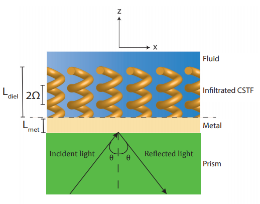
Suppose that a CSTF of thickness is used as the partnering dielectric material in the TKR configuration and the planar metal/prism interface is identified as the plane . The CSTF comprises closely nested nanohelixes of a dielectric material that were grown parallel to each other by the process of physical vapor deposition. The CSTF is infiltrated by a fluid of refractive index which also fills the half space . The prism material is taken to fill the half space . A schematic is provided in Fig. 1.
The anisotropy and nonhomogeneity of the CSTF are macroscopically quantified by the relative permittivity dyadic [29, 54]
| (3) |
Here, the local relative permittivity dyadic
| (4) |
in the material frame captures the local orthorhombicity of the CSTF; the dyadic
| (5) |
captures the rotation of the local relative permittivity dyadic in the laboratory frame about the axis, with denoting the structural handedness and the period; and the dyadic
| (6) |
represents the locally aciculate morphology of the CSTF, with deg being the rise angle with respect to the plane. Both and have the same eigenvalues—denoted by , , and —but their eigenvectors differ. All three parameters of the fluid-infiltrated CSTF depend not only on but also on (which is itself dependent on ) [54]. If are known for at a specific value of , then a combination of inverse and forward Bruggeman homogenization formalisms can be used to deduce their values for at the same [29].
The electric field phasor of the plane wave incident on the prism/metal interface can be written as [54]
| (7) | |||||
where , is the amplitude of the -polarized component and of the -polarized component. The incidence direction is specified by the angles and . The electric field phasor of the reflected plane wave can be written as [54]
| (8) | |||||
where is the amplitude of the -polarized component and of the -polarized component. The reflectance is defined as
| (9) |
2.2 Artificial Neural Networks
ANNs are machine-learning algorithms of a specific type [36]. Machine-learning algorithms are constructed such that they improve in performance over time for a specific task without being explicitly programmed for that task. Typically, an ANN comprises multiple nodes (neurons) organized in several layers arranged in a hierarchy. Each node in a given layer is interconnected with all the nodes in the adjacent layers. These interconnections are represented as numerical values called weights. The designated first layer serves as the input layer and the designated last layer as the output layer. Each node in a given layer computes the linear combination of the value of each node in the previous layer, along with that node’s weight. In order to account for possible non-linear processes, the linear combination is fed into an activation function, such as the sigmoid or rectifier function. A neuron with no activation function is called a linear neuron, and an ANN composed exclusively of linear neurons will fit a linear model to the data.
ANNs require training and testing before implementation. An ANN is trained on a data set of column vectors denoted by , . consists of scalars , . In addition, there are label vectors , each consisting of scalars , . Every is accompanied by a unique , but some of the labels may share the same value when considering noisy data. As an example, two different sensor chips employed in the TKR configuration may produce slightly different reflectance signatures given the same infiltrating liquid, due to differences in sensor-chip quality from the fabrication process.
For a specific , is fed into the input layer, being fed to the node labeled in that layer. With the weights randomized, the label vector is predicted by the ANN and an error value is calculated based on some predefined error function of and . In general, . This error function can be expressed as a function of the weights, since is a function of the weights. Typically, an ANN uses a gradient-descent method [35] to find the weights such that the average error over is sufficiently small. The ANN is then tested on a data set .
In this paper, every testing vector and its elements are identified by the addition of an overbar to the symbol for the corresponding training vector and its elements. In addition, we use with and as placeholders to denote the polarization state (represented by the ratio of to ) and the angle , respectively, of the incident plane wave for which the reflectance data are obtained. This notation is explained in Tables 1 and 2. Next, all styles and fonts of uppercase ‘R’ represent reflectance data calculated for various polarization states, angles , and angles . Finally, all styles and fonts of lowercase ‘n’ represent refractive-index data (i.e., ) corresponding to the reflectance data. Let us note that denotes the refractive index of the infiltrating liquid in general, whether used for training, testing, both, or neither.
| 1 | linear () | ||
| 2 | linear () | ||
| 3 | linear (a mixture of and ) | ||
| 4 | linear (another mixture of and ) | ||
| 5 | left circular | ||
| 6 | right circular |
| (deg) | |
|---|---|
| 1 | |
| 2 | |
| 3 | |
| 4 | |
| 5 | |
| 6 |
Theorems of machine learning suggest that an algorithm tailored to the needs of the specific application must be sought [57, 58]. Therefore, we trained two ANNs with differing structures for various with label vectors and tested the ANNs for various with the label vectors . For this work, both and comprise just one element each (i.e., ) and therefore are denoted simply as and , respectively.
3 Simulations
3.1 Training Data
After fixing nm, various were calculated using a CSTF with half-period nm and thickness nm made of titanium oxide. When , we set , , and , corresponding to , as provided by actual measurements on columnar thin films [59]. Values of for were computed using a homogenization approach detailed elsewhere [29]. Choosing the metal to be silver, we fixed [60] and nm [30]. The prism was chosen to be made of SF11 glass so that . Noting that most applications for biosensors involve small concentrations of analytes dispersed in solvents of refractive index close to that of water (), we chose to calculate various and for for equal increments and , respectively, as determined by . All and were calculated for in steps of , which can be related [31] to by the standard law of refraction, yielding for the prism with a –– triangle as its cross section. All data were computed using Mathematica® running on a laptop computer with a 4-core 2.4-GHz processor and 16 GB of RAM. With , , and fixed, the average estimated computation time was s for the set of six polarization states specified in Table 1.
3.1.1 Training with Incident Light of Diverse Polarization States
SPP-wave modes are capable of being excited by incident light of an arbitrary polarization state in the prism-coupled configuration when a periodically nonhomogeneous dielectric material is partnering a metal thin film [20]. However, experiments have shown that using -polarized incident light results in a higher sensitivity over -polarized incident light, based on the definition [31]
| (10) |
of sensitivity, where , , is the refractive index of an infiltrant fluid labeled and is the value of for . One might then infer that from -polarized incident light will yield better training for an ANN. However, since is focused on SPP-wave modes but not on waveguide modes and other phenomena, as mentioned in Sec. 1, we conjectured that -polarized incident light as well as incident light of other polarization states may also be useful for ANN training.
3.1.2 Training with Light Incident at Diverse
To determine what value of the angle is the most effective, training data sets , , were implemented for separate ANNs. For these sets, we fixed and . For the counterpart testing data sets , , we used and .
3.1.3 Training with Some Combinations of Diverse Polarization States
Even if one polarization state is more effective than the others, the ANN still may benefit from the inclusion of reflectance data from the other polarization states. We use the notation to mean reflectance data that includes polarization states labeled ; thus, and . Fixing , we focused on . For , , , , , and , we have and , and , respectively. Whereas for , , and for , and , respectively.
3.1.4 Training with Some Combinations of Diverse
With similar reasoning as in Sec. 3.1.3, we write to mean reflectance data that includes values of corresponding to ; thus, and . Fixing our attention only on incident -polarized light, we focused on . For , , , , , and , and and , and , respectively. The testing data set was constituted with and , and for , and , respectively.
3.1.5 Training with Combinations of Polarization State and
Of the multitude of reflectance data sets that can be determined for combinations of polarization states and , we only investigated
| (11) |
For this training data set, and . For the corresponding testing data set , and .
3.1.6 Addition of Noise
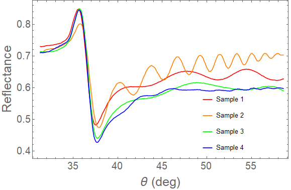
For the data set that yielded the best ANN performance, noise was added to that set to simulate experimental data. The corresponding noisy data set is denoted by with the specific superscript and subscript of the set that yielded the best performance. As shown in Sec. 4, the best-performance set was . The noise was simulated as a random number between and added to each element for different instances. The upper and lower bounds of the random numbers were chosen based on the average absolute difference of reflectance data between four different -nm-thick aluminum films implemented in a specific TKR apparatus, as shown in Fig. 2 . Thus, for , and . For the corresponding testing data set , and .
3.1.7 Training with just SPR data
Up until this stage, each training and testing data set has included reflectance data from ranging from about to about . With inspiration from conventional SPR occurring at the interface of a metal and a homogeneous dielectric material, we devised a data set denoted by with ranging between and in steps of , with , , , , and with no noise added. In order to ensure that only the occurrences of SPR were captured in , the reflectances were calculated with nm and nm, and only those dips that differed by less than for the two values of were retained [30, 31]. Thus most entries in the column vectors in were zero. The corresponding testing data set was constituted with , and . This data set would allow us to to determine the relative efficacy of SPR alone for training ANNs.
3.2 ANN Parameters
All training and testing was done using MATLAB® running on a laptop computer with a 4-core 2.4-GHz processor and 16 GB of RAM. In all, training took no more than a day. Each training data set was used for two separate ANN structures. The first type of ANN structure, denoted by ANN1, consisted of three layers: an input layer, one hidden layer, and an output layer. The hidden layer contained 100 nodes with no activation function (linear neurons) and the output layer contained one node. The second ANN structure, denoted by ANN2 consisted of four layers: an input layer, two hidden layers, and an output layer. The two hidden layers each contained nodes with rectifier activation functions, and the output layer contained one node. The input layer for both ANN1 and ANN2 consisted of one vector. The size of this vector was either , , , , , , , or depending on the specific data set being used for training. The stochastic gradient-descent with momentum method [61] was chosen for optimization with an initial learning rate of and the error function defined as the mean-squared error. The number of maximum epochs was , an epoch being the number of times the learning algorithm was exposed to a given training data set.
The mean , standard deviation , median , maximum , and minimum of for each testing data set were used to assess the performance of each ANN. In addition, for several instances of training for any given ANN with a particular structure and training data set, the performance of that ANN given the same testing data set may vary due to the fact that the weights are randomized at the start of each training instance. Therefore, given a particular training data set, we trained each ANN for ten instances and averaged the aforementioned statistical measures for all of the training instances. Thus, hereafter, the symbols , , , , and , denote performance measures averaged over ten training instances. Ideally, all five performance measures should be as close to as possible.
4 Numerical Results and Discussion
4.1 ANN1
Values of all five performance measures for every training data set for ANN1 are listed in Table 3. This table is divided into six blocks, one each for , , , , , and (, respectively). Within each of the first four blocks, those training sets which yielded the lowest value for each performance measure are highlighted by a colored background. In addition, the overall lowest value for each performance measure is identified in boldface.
| () | () | () | () | () | () | () | () | () | () | ||
| 0.0174 | |||||||||||
| 4.9258 | 4.6006 | 19.7462 | |||||||||
| 3.1690 | |||||||||||
4.2 ANN2
Values of all five performance measures for every training data set for ANN2 are listed in Table 4. This table is divided into six blocks, one each for , , , , , and (, respectively). Within each of the first four blocks, those training sets which yielded the lowest value for each performance measure are highlighted by a colored background. In addition, the overall lowest value for each performance measure is identified in boldface.
| () | () | () | () | () | () | () | () | () | () | ||
| 4.9553 | |||||||||||
| 6.5693 | 5.3522 | 23.8877 | |||||||||
4.3 Comparison of ANN1 and ANN2
Training of ANN1 for each provided a linear function to predict . By having three out of five performance measures as the lowest, we may define as providing the best training for ANN1. We also note that changing does not change the performance of ANN1 as much as changing the polarization state. The same statement goes for the addition of more values versus the addition of more polarization states.
Training of ANN2 for each provided a non-linear function to predict . By having out of performance measures being the lowest, we may define as providing the best training for ANN2. If we compare ANN2 and with ANN1 and , the latter pair perform better, despite the former training set containing more data and the latter ANN having a simpler structure.
Training of ANN1 with yielded , , , , and , while training of ANN2 with yielded , , , , and . Overall, both sets of measures are significantly worse compared to training with any other . We conclude from this that sensing only with SPR data seriously undermines the ability of an ANN to correctly predict .
When noise consistent with actual experimental data was added, we found that the performance of a simple ANN with a small number of training examples yielded no more than a difference between the actual and predicted based on the fact that for ANN1 trained with . Thus, use of ANNs provides a level of immunity to measurement noise.
5 Concluding Remarks
A typical method for sensing is via SPR using the TKR configuration. We have simulated reflectance data from a liquid-infiltrated CSTF partnering a metal thin-film in the TKR configuration and used this data to train two ANNs with differing structures. The performance measures of the ANNs for many training instance were compared. The various training data sets contained reflectance data calculated for various combinations of the polarization state and the angle . Some of this training data was complicated by realistic noise. We stress here that our work pertains directly to the sensing of and only indirectly to the identification of the infiltrant fluid, functionalization [8] being required for the latter purpose.
One main conclusion we have shown is that can best be predicted from -polarized light with , with an ANN having no activation function. This instance represents a best-case scenario. It will require the use of either a triangular prism with a very broad base or a hemispherical prism because the value of is very high.
Another main conclusion of this paper is that the inclusion of other reflectance data in addition to SPR data greatly improves the performance of an ANN. Given the simplicity and heuristic choice of the ANN1 structure and the relative small number of training examples compared to the testing examples used for this work, we are optimistic that significant improvement in the performance can be achieved in the future by adding more training examples and refining the ANN1 structure. Eventually, the application of ANNs may engender an era of simultaneous multianalyte sensing [30]. We also expect our ANN methodology to apply when SPP waves are manipulated by active functional materials and phase-change materials for enhanced sensitivity [62, 63].
Appendix A: MATLAB® codes for Artificial Neural Networks
The variables n and mb represent the input layer size and mini-batch size, respectively. The mini-batch size was that of the training data set used for that instance.
A.1: ANN1
layers = [ ...
    sequenceInputLayer(n)
    fullyConnectedLayer(100)
    fullyConnectedLayer(1)
    regressionLayer];
options = trainingOptions(’sgdm’,’InitialLearnRate’,0.01, ...
    ’MaxEpochs’,10000,...
    ’MiniBatchSize’,mb)
A.2: ANN2
    layers = [ ...
        sequenceInputLayer(n)
        fullyConnectedLayer(100)
        reluLayer
        fullyConnectedLayer(100)
        reluLayer
        fullyConnectedLayer(1)
        regressionLayer];
    options = trainingOptions(’sgdm’,’InitialLearnRate’,0.01, ...
        ’MaxEpochs’,10000,...
        ’MiniBatchSize’,mb)
Acknowledgments. The research of P. D. McAtee and A. Lakhtakia is funded by the Charles Godfrey Binder Endowment at the Pennsylvania State University.
References
- [1] C. McDonagh, C. S. Burke, and B. D. MacCraith, “Optical chemical sensors,” Chemical Reviews 108, 400–422 (2008). [doi: 10.1021/cr068102g].
- [2] A. P. F. Turner, “Biosensors: sense and sensibility,” Chemical Society Reviews 42, 3184–3196 (2013). [doi: 10.1039/c3cs35528d].
- [3] D. V. Lim, J. M. Simpson, E. A. Kearns, and M. F. Kramer, “Current and developing technologies for monitoring agents of bioterrorism and biowarfare,” Clinical Microbiology Reviews 18, 583–607 (2005). [doi: 10.1128/CMR.18.4.583-607.2005].
- [4] N. Verma and A. Bhardwaj, “Biosensor technology for pesticides—A review,” Applied Biochemistry and Biotechnology 175, 3093–3119 (2014). [doi: 10.1007/s12010-015-1489-2].
- [5] A. Orlando, M. Colombo, D. Prosperi, F. Corsi, A. Panariti, I. Rivolta, M. Masserini, and E. Cazzaniga, “Evaluation of gold nanoparticles biocompatibility: a multiparametric study on cultured endothelial cells and macrophages,” Journal of Nanoparticle Research 18, 58 (2016). [doi: 10.1007/s11051-016-3359-4].
- [6] I. Fratoddi, I. Venditti, C. Cametti, and M. V. Russo, “How toxic are gold nanoparticles? The state of the art,” Nano Research 8, 1771–1799 (2015). [doi: 10.1007/s12274-014-0697-3].
- [7] A. M. Alkilany and C. J. Murphy, “Toxicity and cellular uptake of gold nanoparticles: what have we learned so far?,” Journal of Nanoparticle Research 12, 2313–2333 (2010). [doi: 10.1007/s11051-010-9911-8].
- [8] J. Homola, “Surface plasmon resonance sensors for detection of chemical and biological species,” Chemical Reviews 108, 462–493 (2008). [doi: 10.1021/cr068107d].
- [9] H. Malekzad, P. S. Zangabad, H. Mohammad, M. Sadroddini, Z. Jafari, N. Mahlooji, S. Abbaspour, S. Gholami, M. G. Houshangi, R. Pashazadeh, A. Beyzavi, M. Karimi, and M. R. Hamblin, “Noble metal nanostructures in optical biosensors: Basics, and their introduction to anti-doping detection,” Trends in Analytical Chemistry 100, 116–135 (2018). [doi: 10.1016/j.trac.2017.12.006].
- [10] J. R. Stetter and J. Li, “Amperometric gas sensors—A review,” Chemical Reviews 108, 352–366 (2008). [doi: 10.1021/cr0681039].
- [11] S. Cosnier, Electrochemical Biosensors, Pan Stanford, New York (2015).
- [12] I. Abdulhalim, M. Zourob, and A. Lakhtakia, “Surface plasmon resonance for biosensing: A mini-review,” Electromagnetics 28, 214–242 (2008). [doi: 10.1080/02726340801921650].
- [13] T. Taliercio, F. G.-P. Flores, F. B. Barho, M. J. Milla–Rodrigo, M. Bomers, L. Cerutti, and E. Tournié, “Plasmonic bio-sensing based on highly doped semiconductors,” Proceedings of SPIE 10353, 103530S (2017). [doi: 10.1117/12.2274303].
- [14] M. Arjmand, H. Saghafifar, M. Alijanianzadeh, and M. Soltanolkotabi, “A sensitive tapered-fiber optic biosensor for the label-free detection of organophosphate pesticides,” Sensors and Actuators B: Chemical 249, 523–532 (2017). [doi: 10.1016/j.snb.2017.04.121].
- [15] P. Skládal, “Piezoelectric biosensors,” Trends in Analytical Chemistry 79, 127–133 (2016). [doi: 10.1016/j.trac.2015.12.009].
- [16] M. DeMiguel–Ramos, B. Díaz–Durán, J.-M. Escolano, M. Barba, T. Mirea, J. Olivares, M. Clement, and E. Iborra, “Gravimetric biosensor based on a 1.3 GHz AlN shear-mode solidly mounted resonator,” Sensors and Actuators B: Chemical 239, 1282–1288 (2017). [doi: 10.1016/j.snb.2016.09.079].
- [17] A. Davidson, A. Buis, and I. Glesk, “Toward novel wearable pyroelectric temperature sensor for medical applications,” IEEE Sensors Journal 17, 6682–6689 (2017). [doi:10.1109/JSEN.2017.2744181].
- [18] A. Rasooly and K. E. Herold (eds.), Biosensors and Biodetection: Methods and Protocols, Volume 503: Optical-Based Detectors, Humana Press, New York (2009).
- [19] M. Zourob and A. Lakhtakia (eds.), Optical Guided-wave Chemical and Biosensors, Vols. 1 and 2, Springer, Heidelberg, Germany (2010).
- [20] J. A. Polo Jr., T. G. Mackay, and A. Lakhtakia, Electromagnetic Surface Waves: A Modern Perspective, Elsevier, Waltham, Massachusetts (2013).
- [21] H. J. Simon, D. E. Mitchell, and J. G. Watson, “Surface plasmons in silver films—a novel undergraduate experiment,” American Journal of Physics 43, 630–636 (1975). [doi: 10.1119/1.9764].
- [22] T. Turbadar, “Complete absorption of light by thin metal films,” Proceedings of the Physical Society 73, 40–44 (1959). [doi: 10.1088/0370-1328/73/1/307].
- [23] E. Kretschmann and H. Raether, “Radiative decay of non radiative surface plasmons excited by light,” Zeitschrift für Naturforschung A 23, 2135–2136 (1968). [doi: 10.1515/zna-1968-1247].
- [24] G. J. Sprokel, “The reflectivity of a liquid crystal cell in a surface plasmon experiment,” Molecular Crystals and Liquid Crystals 68, 39–45 (1981). [doi: 10.1080/00268948108073551].
- [25] G. J. Sprokel, R. Santo, and J. D. Swalen, “Determination of the surface tilt angle by attenuated total reflection,” Molecular Crystals and Liquid Crystals 68, 29–38 (1981). [doi:10.1080/00268948108073550].
- [26] Devender, D. P Pulsifer, and A. Lakhtakia, “Multiple surface plasmon polariton waves,” Electronics Letters 45, 1137–1138 (2009). [doi:10.1117/1.3249629].
- [27] A. Lakhtakia, Y.-J. Jen, and C.-F. Lin, “Multiple trains of same-color surface plasmon-polaritons guided by the planar interface of a metal and a sculptured nematic thin film. Part III: Experimental evidence,” Journal of Nanophotonics 3, 033506 (2009). [doi: 10.1117/1.3249629].
- [28] T. H. Gilani, N. Dushkina, W. L. Freeman, M. Z. Numan, D. N. Talwar, and D. P. Pulsifer, “Surface plasmon resonance due to the interface of a metal and a chiral sculptured thin film,” Optical Engineering 49, 120503 (2010). [doi: 10.1117/1.3525282].
- [29] T. G. Mackay and A. Lakhtakia, “Modeling chiral sculptured thin films as platforms for surface-plasmonic-polaritonic optical sensing,” IEEE Sensors Journal 12, 273–280 (2012). [doi: 10.1109/JSEN.2010.2067448].
- [30] S. E. Swiontek, D. P. Pulsifer, and A. Lakhtakia, “Optical sensing of analytes in aqueous solutions with multiple surface-plasmon-polariton-wave platform,” Scientific Reports 3, 1409 (2013). [doi: 10.1038/srep01409].
- [31] S. E. Swiontek and A. Lakhtakia, “Influence of silver-nanoparticle layer in a chiral sculptured thin film for surface-multiplasmonic sensing of analytes in aqueous solution,” Journal of Nanophotonics 10, 033008 (2016). [doi: 10.1117/1.JNP.10.033008].
- [32] D. Marcuse, Theory of Dielectric Optical Waveguides, Academic Press, San Diego, California (1991).
- [33] T. Khaleque and R. Magnusson, “Light management through guided-mode resonances in thin-film silicon solar cells,” Journal of Nanophotonics 8, 083995 (2014). [doi: 10.1117/1.JNP.8.083995].
- [34] L. Liu, M. Faryad, A. S. Hall, G. D. Barber, S. Erten, T. E. Mallouk, A. Lakhtakia, and T. S. Mayer, “Experimental excitation of multiple surface plasmon-polariton waves and waveguide modes in a one-dimensional photonic crystal atop a two-dimensional metal grating,” Journal of Nanophotonics 9, 093593 (2015). [doi: 10.1117/1.JNP.9.093593].
- [35] D. E. Rumelhart, G. E. Hinton, and R. J. Williams, “Learning internal representations by error propagation,” In: D. E. Rumelhart and J. L. McClelland (eds), Parallel Distributed Processing: Explorations in the Microstructure of Cognition. Volume 1: Foundations, pp. 318–362, MIT Press, Cambridge, Massachusetts (1986).
- [36] I. Goodfellow, Y. Bengio, and A. Courville, Deep Learning, MIT Press, Cambridge, Massachusetts (2016).
- [37] S. T. S. Bukkapatnam, A. Lakhtakia, and S. R. T. Kumara, “Chaotic neurons for on-line quality control in manufacturing,” International Journal of Advanced Manufacturing Technology 13, 95–100 (1997). [doi: 10.1007/BF01225755].
- [38] S. T. S. Bukkapatnam, S. R. T. Kumara, and A. Lakhtakia, “Fractal estimation of flank wear in turning,” Journal of Dynamic Systems, Measurement, and Control 122, 89–94 (2000). [doi: 10.1115/1.482446].
- [39] S. T. S. Bukkapatnam, S. R. T. Kumara, and A. Lakhtakia, “Analysis of acoustic emission signals in machining,” Journal of Manufacturing Science and Engineering 121, 568–576 (1999). [doi: 10.1115/1.2833058].
- [40] S. T. S. Bukkapatnam, A. Lakhtakia, and S. R. T. Kumara, “Analysis of sensor signals shows turning on a lathe exhibits low-dimensional chaos,” Physical Review E 152, 2375–2387 (1995). [doi:10.1103/PhysRevE.52.2375].
- [41] J. J. Braun, Y. Glina, J. K. Su, and T. J. Dasey, “Computational intelligence in biological sensing,” Proceedings of SPIE 5416, 111–122 (2004). [doi: 10.1117/12.541046].
- [42] S. Chakrabartty and Y. Liu, “Towards reliable multi-pathogen biosensors using high-dimensional encoding and decoding techniques,” Proceedings of SPIE 7035, 703514 (2008). [doi: 10.1117/12.799358].
- [43] V. A. Saetchnikov, E. A. Tcherniavskaia, G. Schweiger, and A. Ostendorf, “Classification of antibiotics by neural network analysis of optical resonance data of whispering gallery modes in dielectric microspheres,” Proceedings of SPIE 8424, 84240Q (2012). [doi: 10.1117/12.920397].
- [44] P. H. Rogers, K. D. Benkstein, and S. Semancik, “Machine learning applied to chemical analysis: Sensing multiple biomarkers in simulated breath using a temperature-pulsed electronic-nose,” Analytical Chemistry 84, 9774–9781 (2012). [doi: 10.1021/ac301687j].
- [45] N. Maleki, S. Kashanian, E. Maleki, and M. Nazari, “A novel enzyme based biosensor for catechol detection in water samples using artificial neural network,” Biochemical Engineering Journal 128, 1–11 (2017). [doi: 10.1016/j.bej.2017.09.005].
- [46] K. N. Mutter, “Hopfield neural network and optical fiber sensor as intelligent heart rate monitor,” Proceedings of SPIE 10456, 104564T (2018). [doi: 10.1117/12.2283012].
- [47] W. Ma, F. Cheng, and Y. Liu, “Deep-learning-enabled on-demand design of chiral metamaterials,” ACS Nano 12, 6326–6334 (2018). [doi: 10.1021/acsnano.8b03569].
- [48] D. Liu, Y. Tan, E. Khoram, and Z. Yu, “Training deep neural networks for the inverse design of nanophotonics structures,” ACS Photonics 5, 1365–1369 (2018). [doi: 10.1021/acsphotonics.7b01377].
- [49] M. R. H. Nezhad, J. Tashkhourian, J. Khodaveisi, and M. R. Khoshi, “Simultaneous colorimetric determination of dopamine and ascorbic acid based on the surface plasmon resonance band of colloidal silver nanoparticles using artificial neural networks,” Analytical Methods 2, 1263–1269 (2010). [doi: 10.1039/C0AY00302F].
- [50] J. Ma, Y. Cao, K. Liu, X. Huang, J. Jiang, T. Wang, M. Xue, P. Chang, and T. Liu, ‘ “A simple demodulation algorithm for optical SPR sensor based on all-phase low-pass filters,” Proceedings of SPIE 10618, 106180N (2018). [doi: 10.1117/12.2281236].
- [51] J. Khodaveisi, S. Dadfarnia, A. M. H. Shabani, M. R. Moghadam, and M. R. H. Nezhad, “Artificial neural network assisted kinetic spectrophotometric technique for simultaneous determination of paracetamol and p-aminophenol in pharmaceutical samples using localized surface plasmon resonance band of silver nanoparticles,” Spectrochimica Acta Part A: Molecular and Biomolecular Spectroscopy 138, 474–480 (2015). [doi: 10.1016/j.saa.2014.11.094].
- [52] S. Yu, J. Wang, T. Zhang, R. Zhou, J. Dai, Y. Zhou, and K. Xu, “Performance optimization for plasmonic refractive index sensor based on machine learning ,” Proceedings of SPIE 11048, 110482X (2019). [doi: 10.1117/12.2519699].
- [53] F. Bahrami, M. Maisonneuve, M. Meunier, J. S. Aitchison, and M. Mojahedi, “An improved refractive index sensor based on genetic optimization of plasmon waveguide resonance,” Optics Express 21, 20863–20872 (2013). [doi: 10.1364/OE.21.020863].
- [54] A. Lakhtakia, “Enhancement of optical activity of chiral sculptured thin films by suitable infiltration of void regions,” Optik 112, 145–148 (2001). [doi: 10.1078/0030-4026-00024].
- [55] A. Lakhtakia, “Erratum: Enhancement of optical activity of chiral sculptured thin films by suitable infiltration of void regions,” Optik 112, 544 (2001). [doi: 10.1078/0030-4026-00024].
- [56] P. D. McAtee, S. T. S. Bukkapatnam, and A. Lakhtakia, “Artificial neural network to predict the refractive index of a liquid infiltrating a chiral sculptured thin film,” Proceedings of SPIE 10728, 107280G (2018). [doi: 10.1117/12.2321355].
- [57] D. H. Wolpert, “The lack of a priori distinctions between learning algorithms,” Neural Computation 8, 1341–1390 (1996). [doi: 10.1162/neco.1996.8.7.1341].
- [58] D. H. Wolpert and W. G. Macready, “No free lunch theorems for optimization,” IEEE Transactions on Evolutionary Computation 1, 67–82 (1997). [doi: 10.1109/4235.585893].
- [59] I. Hodgkinson, Q. h. Wu, and J. Hazel, “Empirical equations for the principal refractive indices and column angle of obliquely deposited films of tantalum oxide, titanium oxide, and zirconium oxide,” Applied Optics 37, 2653–2659 (1998). [doi: 10.1364/AO.37.002653].
- [60] https://refractiveindex.info/?shelf=main&book=Au&page=Johnson (accessed on July 11 2018).
- [61] J. Patterson and A. Gibson, Deep Learning, O’Reilly Media, Sebastopol, California (2017).
- [62] D. Rodrigo, O. Limaj, D. Janner, D. Etezadi, F. J. García de Abajo, V. Pruneri, and H. Altug, “Mid-infrared plasmonic biosensing with graphene,” Science 349, 165–168 (2015). [doi: 10.1126/science.aab2051].
- [63] K. V. Sreekanth, Q. Ouyang, S. Sreejith, S. Zeng, W. Lishu, E. Ilker, W. Dong, M. ElKabbash, Y. Ting C. T. Lim, M. Hinczewski, G. Strangi, K.-T. Yong, R. E. Simpson, and R. Singh, “Phase-change-material-based low-loss visible-frequency hyperbolic metamaterials for ultrasensitive label-free biosensing,” Advanced Optical Materials 7, 1900081 (2019). [doi: 10.1002/adom.201900081].