Aligning Linguistic Words and Visual Semantic Units
for Image Captioning

Abstract.

Image captioning attempts to generate a sentence composed of several linguistic words, which are used to describe objects, attributes, and interactions in an image, denoted as visual semantic units in this paper. Based on this view, we propose to explicitly model the object interactions in semantics and geometry based on Graph Convolutional Networks (GCNs), and fully exploit the alignment between linguistic words and visual semantic units for image captioning. Particularly, we construct a semantic graph and a geometry graph, where each node corresponds to a visual semantic unit, i.e., an object, an attribute, or a semantic (geometrical) interaction between two objects. Accordingly, the semantic (geometrical) context-aware embeddings for each unit are obtained through the corresponding GCN learning processers. At each time step, a context gated attention module takes as inputs the embeddings of the visual semantic units and hierarchically align the current word with these units by first deciding which type of visual semantic unit (object, attribute, or interaction) the current word is about, and then finding the most correlated visual semantic units under this type. Extensive experiments are conducted on the challenging MS-COCO image captioning dataset, and superior results are reported when comparing to state-of-the-art approaches. The code is publicly available at https://github.com/ltguo19/VSUA-Captioning.

1. Introduction

Computer vision and natural language processing are becoming increasingly intertwined. At the intersection of the two subjects, automatically generating lingual descriptions of images, namely image captioning (Vinyals et al., 2017; Karpathy and Feifei, 2015; Fang et al., 2014), has emerged as a prominent interdisciplinary research problem. Modern image captioning models typically employ an encoder-decoder framework, where the encoder encodes an image into visual representations and then the decoder decodes them into a sequence of words.

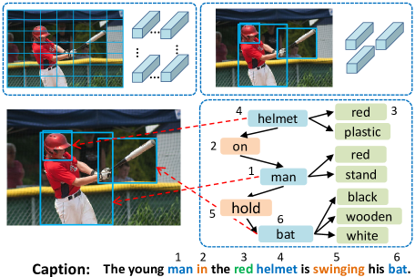
Figure 1. Typically, image captioning models consider the visual content of images as uniform grids (top left) or collections of object regions (top right). Differently, our approach represents images as structured graphs where nodes are VSUs: object, attribute, and relationship units (bottom). We make use of the alignment nature between caption words and VSUs.

How to represent visual content and how to reason over them are fundamental problems in image captioning. Starting from the static, single-vector representations, the visual representations have evolved into using dynamic, multi-vector representations, which are often fed into an attention module for information aggregation. In the early times, the image is treated as uniform grid representations, then more recently, state-of-the-art methods regard visual content as collections of individual object regions (the top row in Figure 1). However, the isolated objects only represent the categories and properties of individual instances, which are often related to nouns or noun phrases in a caption, but fail to model object-object relations, e.g. the interactions or relative positions. While the relationships between objects are the natural basis for describing an image.

In fact, the image is a structured combination of objects (“man”, “helmet”), their attributes (“helmet is red”), and more importantly, relationships (“man hold bat”) involving these objects. We call these visual components visual semantic units (VSUs) in this paper, which include three categories: object units, attribute units, and relationship units. At the same time, a sentence is also composed of syntactic units describing objects (e.g. nouns phrase), their properties (e.g. adjectives) and relations (e.g. verb, prepositions). Because captions are abstractions of images, it is intuitive that each word in the caption can roughly be aligned with the VSUs of the image. Exploiting such vision-language correlation could benefit image understanding and captioning.

In this paper, we propose to represent visual content with VSU-based structured graphs, and take advantage of the strong correlations between linguistic syntactic units and VSUs for image captioning. First, we detect a collection of VSUs from the image through object, attribute, and relationship detectors, respectively. Then we construct structured graphs as explicit and unified representation that connects the detected objects, attributes, and relationships (e.g. bottom-right in Figure 1), where each node corresponds to a VSU and the edges are the connections between two VSUs. In particular, we construct a semantic graph and a geometry graph, where the former models the semantic relationships (e.g. “man holding bat”) and the latter models the geometry relationships (e.g. “the man the and bat are adjacent and overlapped”). After that, Graph Convolutional Networks (GCNs) are then explored to learn context-aware embeddings for each VSU in the graph.

We design a context gated attention module (CGA) that attends to the three types of VSUs in a hierarchical manner when generating each caption word. The key insight behind CGA is that each word in the caption could be aligned with a VSU, and if the word is about objects, e.g. a noun, then the corresponding VSU should also be an object unit, meaning that more attention should be paid on the object units. Specifically, CGA first performs three independent attention mechanism inside the object, attribute, and relationship units, respectively. Then a gated fusion process is performed to adaptively decide how much attention should be paid to each of the three VSU categories by referring to the current linguistic context. Knowledge learned from the semantic graph and the geometry graph are naturally fused by extending CGA’s input components to include the VSUs from both graphs.

The main contributions of this paper are three-fold.

• We introduce visual semantic units as comprehensive representation of the visual content, and exploit structured graphs, i.e. semantic graph and geometry graph, and GCNs to uniformly represent them.

• We explore the vision-language correlation and design a context gated attention module to hierarchically align linguistic words and visual semantic units.

• Extensive experiments on MS COCO validates the superiority of our method. Particularly, in terms of the popular CIDEr-D metric, we achieve an absolute $8.5$ points improvement over the strong baseline, i.e. Up-Down (Anderson et al., 2017), on Karpathy test split.

2. Related Work

Image Captioning.

Filling the information gap between the visual content of the images and their corresponding descriptions is a long-standing problem in image captioning. Based on the encoder-decoder pipeline (Vinyals et al., 2015; Yang et al., 2016; You et al., 2016), much progress has been made on image captioning. For example, (Xu et al., 2015) introduces the visual attention that adaptively attends to the salient areas in the image, (Lu et al., 2017) proposes an adaptive attention model that decides whether to attend to the image or to the visual sentinel, (Yang et al., 2019) corporates learned language bias as a language prior for more human-like captions, (Luo et al., 2018) and (Guo et al., 2019) focus on the discriminability and style properties of image captions respectively, and (Rennie et al., 2017) adopts reinforcement learning (RL) that directly optimize evaluation metric.

Recently, some works have been proposed to encode more discriminative visual information into captioning models. For instances, Up-Down (Anderson et al., 2017) extracts region-level image features for training, (Yao et al., 2016) incorporates image-level attributes into the encoder-decoder framework by training a Multiple Instance Learning (Fang et al., 2014) based attribute detectors. However, all these works focus on representing visual content with either objects/grids or global attributes, but fail to model object-object relationships. Differently, our method simultaneously models objects, the instance-level attributes, and relationships with structured graph of VSUs.

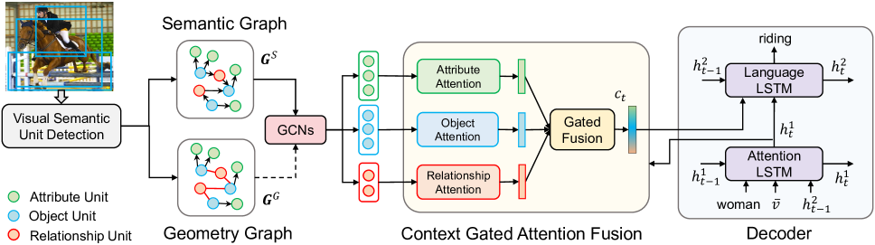
Figure 2. Overview of our method. Given an image, we represent it as structured graphs of visual semantic units (objects, attributes, and relationships in the image) and generate a caption based on them.

Scene Graphs Generation and GCNs.

Recently, inspired by representations studied by the graphics community, (Johnson et al., 2015) introduced the problem of generating scene graphs from images, which requires detecting objects, attributes, and relationships of objects. Many approaches have been proposed for the detection of both objects and their relationships (Xu et al., 2017; Yang et al., 2018; Zellers et al., 2018). Recently, some works have been proposed that leverage scene graph for improving scene understanding in various tasks, e.g. visual question answering (Teney et al., 2017), referring expression understanding (Nagaraja et al., 2016), image retrieval (Johnson et al., 2015), and visual reasoning (Chen et al., 2018). In these works, GCNs (Kipf and Welling, 2016; Gilmer et al., 2017; Bastings et al., 2017) are often adopted to learn node embeddings. A GCN is a multilayer neural network that operates directly on a graph, in which information flows along edges of the graph.

More similar to our work, GCN-LSTM (Yao et al., 2018) refines the region-level features by leveraging object relationships and GCN. However, GCN-LSTM treats relationships as edges in the graph, which are implicitly encoded in the model parameters. While instead, our method considers relationships as additional nodes in the graph and thus can explicitly model relationships by learning instance-specific representations for them.

3. Approach

3.1. Problem Formulation

Image captioning models typically follow the encoder-decoder framework. Given an image $I$, the image encoder $\mathcal{E}$ is used to obtain the visual representation $V=\left\{v_{1},\dots,v_{k}\right\},v_{i}\in\mathbb{R}^{D}$, where each $v_{i}$ represents some features about the image content. Based on $V$, the caption decoder $\mathcal{D}$ generates a sentence $y$ by:

(1) $$V=\mathcal{E}(I),\ \ y=\mathcal{D}(V).$$

The objective of image captioning is to minimize a cross entropy loss.

How to define and represent $V$ is a fundamental problem in this framework. In this work, we consider the visual content as structured combinations of the following three kinds of VSUs:

• Object units ($O$): the individual object instances in the image.

• Attribute units ($A$): the properties following each object.

• Relationship units ($R$): the interactions between object pairs.

That is, we define $V=V_{o}\cup V_{a}\cup V_{r}$, where $V_{o},V_{a}$, and $V_{r}$ denote the collections of visual representations for $O,A$, and $R$, respectively.

The overall framework of our method is shown in Figure 2. First, we detect $O$, $A$, and $R$ from the image with object, attribute, and relationship detectors respectively, based on which, a semantic graph and a geometry graph are constructed by regarding each VSU as the nodes and the connections between two VSUs as the edges. Then, GCNs are applied to learn context-aware embeddings for each of the nodes/VSUs. Afterward, a context gated attention fusion module is introduced to hierarchically align each word with the embedded VSUs, and the resulting context vector is fed into a language decoder for predicting words.

3.2. Graph Representations of Visual Semantic Units

Visual Semantic Units Detection.

We first detect the three types of VSUs by an object detector, an attribute classifier, and a relationship detector respectively, following (Yang et al., 2019). Specifically, Faster R-CNN (Ren et al., 2015) is adopted as the object detector. Then, we train an attribute classifier to predict the instance attributes for each detected object, which is a simple multi-layer perceptron (MLP) network followed by a softmax function. MOTIFNET (Zellers et al., 2018) is adopted as the semantic relationship detector to detect pairwise relationships between object instances using the publicly available code. Finally, we obtain a set of objects, attributes, and relationships, i.e. the VSUs ($O$, $A$, and $R$). We denote $o_{i}$ as the $i$-th object, $a_{i,k}$ as the $k$-th attribute of $o_{i}$, and $r_{ij}$ as the relationship between $o_{i}$ and $o_{j}$. $<$$o_{i},r_{ij},o_{j}$$>$ forms a triplet, which means $<$subject, predicate, object$>$.

Graph Construction.

It is intuitive to introduce graph as a structured representation of the VSUs, which contains nodes and edges connecting them. We can naturally regard both objects and attributes as nodes in the graph, where each attribute node $a_{i,k}$ is connected with the object node $o_{i}$ with a directed edge ($o_{i}\to a_{i,k}$), meaning “object $o_{i}$ owns attribute $a_{i,k}$”. However, whether to represent relationships as edges or nodes in the graph remains uncertain. A common and straightforward solution is to represent relationships as edges connecting pairwise object nodes in the graph (Yao et al., 2018; Teney et al., 2017) (the left side of Figure 3.). However, such models only learn vector representation for each node (objects) and implicitly encode edge (relationships) information in the form of GCN parameters, while the relationship representations are not directly modeled.

Ideally, relationships should have instance-specific representations, in the same way as objects, and they should also inform decisions made in the decoder. Thus, we propose to explicitly modeling relationship representations by turning the relationships as additional nodes in the graph. Concretely, for each relationship $r_{ij}$, we add a node in the graph and draw two directed edges: $o_{i}\to r_{ij}$ and $r_{ij}\to o_{j}$. The subgraph of all $o_{i}$ and $r_{ij}$ is now a bipartite. An instance is shown in the right side of Figure 3.

Formally, given three sets of object nodes (units) $O=\{o_{i}\}$, attribute nodes (units) $A=\{a_{i,k}\}$, and relationship nodes (units) $R=\{r_{ij}\}$, we define the graph $\mathcal{G}=(\mathcal{N},\mathcal{E})$ as comprehensive representation of the visual content for the image, where $\mathcal{N}=O\cup A\cup R$ is the nodes and $\mathcal{E}$ is a set of directed/undirected edges.

Semantic Graph and Geometry Graph.

We consider two types of visual relationships between objects in the image: semantic relationship and geometry relationship, which result in two kinds of graphs, i.e. semantic graph $\mathcal{G}^{S}$ and geometry graph $\mathcal{G}^{G}$. The semantic relationship $R^{S}$ unfolds the inherent action/interaction between objects, e.g. “woman riding horse”. Semantic relationships are detected using MOTIFNET. Geometry relationship $R^{G}$ between objects is an important factor in visual understanding that connects isolated regions together, e.g. “woman on horse”. Here we consider the undirected relative spatial relationships $<$$o_{i^{\prime}},r_{i^{\prime}j^{\prime}},o_{j^{\prime}}$$>$, where $o_{i^{\prime}}$ is the one with larger size between $o_{i}$ and $o_{j}$, while $o_{j^{\prime}}$ is the smaller one. Instead of using a fully connected graph, we assign geometry relationships between two objects if their Intersection over Union (IoU) and relative distance are within given thresholds.

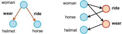
Figure 3. Comparison between regarding relationships as edges and as nodes in the graph. The attribute nodes are omitted for clarity.

3.3. Embedding Visual Semantic Units with GCN

Node Features.

We integrate three kinds of content cues for $o_{i},a_{i,k}$, and $r_{ij}$, i.e. visual appearance cue, semantic embedding cue, and geometry cue.

Visual Appearance Cue. Visual appearance contains delicate details of the object and is a key factor for image understanding. We use the region-level RoI feature from Faster R-CNN as the visual appearance cue for each object, which is a 2048-dimensional vector, denoted as $\boldsymbol{f}^{v}_{o_{i}}$.

Semantic Embedding Cue. The content of objects, attributes and relationships can largely be described with their categories. Thus, we introduce their category labels as the semantic information, which are obtained from the outputs of object, attribute and relationship detectors. Specifically, we use three independent and trainable word embedding layers to maps the object categories into feature embedding vectors (denoted as $\boldsymbol{f}^{s}_{o_{i}},\boldsymbol{f}^{s}_{a_{i,k}}$, and $\boldsymbol{f}^{s}_{r_{ij}}$) for $o_{i},a_{i,k}$, and $r_{ij}$, respectively.

Geometry Cue. Geometry information is complementary to visual appearance information, as it reflects the spatial patterns of individual objects or the relation between two objects. Denote the box of a localized object $o_{i}$ as $(x_{i},y_{i},w_{i},h_{i})$, where $(x_{i},y_{i})$ are the coordinates of the center of the box, and $(w_{i},h_{i})$ are its width and height, and denote the width and height of the image as $(w,h)$. We encode the relative geometric cue of $o_{i}$ with a 5-dimensional vector:

(2) $$\boldsymbol{f}^{g}_{o_{i}}=\big{[}\frac{x_{i}}{w},\frac{y_{i}}{h},\frac{w_{i}}{w},\frac{h_{i}}{h},\frac{w_{i}h_{i}}{wh}\big{]}.$$

We encode the geometric cue of each relationship $r_{ij}$ with a 8-dimensional vector:

$$\boldsymbol{f}^{g}_{r_{ij}}= \Big{[}\underbrace{\frac{x_{j}-x_{i}}{\sqrt{w_{i}h_{i}}},\frac{y_{j}-y_{i}}{\sqrt{w_{i}h_{i}}}}_{r_{1}},\ \underbrace{\frac{w_{j}}{w_{i}},\frac{h_{j}}{h_{i}},\frac{w_{j}h_{j}}{w_{i}h_{i}}}_{r_{2}},\ \underbrace{\frac{o_{i}\cap o_{j}}{o_{i}\cup o_{j}}}_{r_{3}},\$$

(3) $$\underbrace{\frac{\sqrt{(x_{j}-x_{i})^{2}+(y_{j}-y_{i})^{2}}}{\sqrt{w^{2}+h^{2}}}}_{r_{4}},\ \underbrace{atan2(\frac{y_{j}-y_{i}}{x_{j}-x_{i}})}_{r_{5}}\Big{]},$$

where $r_{1}$ represents the normalized translation between the two boxes, $r_{2}$ is the ratio of box sizes, $r_{3}$ is the IoU between boxes, $r_{4}$ is the relative distance normalized by diagonal length of the image, $r_{5}$ is the relative angle $\theta\in(-\pi,\pi]$ between the two boxes.

We fuse the visual appearance cues, semantic embedding cues, and geometry cues to obtain the features for each node/VSU. We aggregate the top-$N_{a}$ predicted attributes $[a_{i,1},...,a_{i,N_{a}}]$ (sorted by the classification confidences) of $o_{i}$ into a single attribute unit $a_{i}$ for each object. Denote the features corresponding to $o_{i},a_{i,k}$, and $r_{ij}$ nodes as $\boldsymbol{f}_{o_{i}},\boldsymbol{f}_{a_{i}}$, and $\boldsymbol{f}_{r_{ij}}$, respectively, and use superscripts $\boldsymbol{f}^{G}$ and $\boldsymbol{f}^{S}$ to denote the features of $\mathcal{G}^{S}$ and $\mathcal{G}^{G}$. The feature of $o_{i}$, $a_{i}$, $r_{ij}$ are given by:

(4) $$\boldsymbol{f}_{o_{i}}=\phi_{o}([\boldsymbol{f}^{v}_{o_{i}};\boldsymbol{f}^{s}_{o_{i}};\boldsymbol{f}^{g}_{o_{i}}]),$$

(5) $$\boldsymbol{f}_{a_{i}}=\phi_{a}([\boldsymbol{f}^{s}_{a_{i,1}};\ldots;\boldsymbol{f}^{s}_{a_{i,N_{a}}}]),$$

(6) $$\boldsymbol{f}^{S}_{r_{ij}}=\phi_{r}(\boldsymbol{f}^{s}_{r_{ij}}),$$

(7) $$\boldsymbol{f}^{G}_{r_{ij}}=\phi_{r}(\boldsymbol{f}^{g}_{r_{ij}}),$$

where $[*;*]$ means concatenation operation, and $\phi_{o},\phi_{a}$, and $\phi_{r}$ are feature projection layers which are all implemented as FC-ReLU-Dropout.

Node Embedding with GCNs.

After obtaining the features for the three kinds of nodes/VSUs, we then adopt GCNs: $g_{o},g_{a}$, and $g_{r}$, to learn semantic (geometrical) context-aware embeddings for the $o_{i},a_{i}$, and $r_{ij}$ nodes in $\mathcal{G}$, respectively.

The object unit embedding $\boldsymbol{u}_{o_{i}}$ is calculated as:

(8) $$\boldsymbol{u}_{o_{i}}=g_{o}(\boldsymbol{f}_{o_{i}})+\boldsymbol{f}^{v}_{o_{i}},$$

where adding $\boldsymbol{f}^{v}_{o_{i}}$ serves as a kind of “residual connection”, which we empirically found helpful for model performance.

Given the feature $\boldsymbol{f}_{a_{i}}$ of an attribute unit $a_{i}$, we integrate it with its object context $o_{i}$ for calculating the attribute unit embedding $\boldsymbol{u}_{a_{i}}$ by:

(9) $$\boldsymbol{u}_{a_{i}}=g_{a}\left(\boldsymbol{u}_{o_{i}},\boldsymbol{f}_{a_{i}}\right)+\boldsymbol{f}_{a_{i}}.$$

For each relationship $r_{ij}$ and its associated relationship triplet $<$$o_{i},r_{ij},o_{j}$$>$, we aggregate the information from its neighboring nodes ($o_{i}$ and $o_{j}$) to calculate the relationship unit embedding $u_{r_{ij}}$ by:

(10) $$\boldsymbol{u}_{r_{ij}}=g_{r}\left(\boldsymbol{u}_{o_{i}},\boldsymbol{f}_{r_{ij}},\boldsymbol{u}_{o_{j}}\right)+\boldsymbol{f}_{r_{ij}}.$$

In our implementation, $g_{o},g_{a}$, and $g_{r}$ use the same structure with independent parameters: a concatenation operation followed by a FC-ReLU-Dropout layer. Note that for $\mathcal{G}^{S}$ and $\mathcal{G}^{G}$, their $\boldsymbol{u}_{o_{i}}$ and $\boldsymbol{u}_{a_{i}}$ are the same, while their $\boldsymbol{u}_{r_{ij}}$ are independently calculated and denoted as $\boldsymbol{u}^{S}_{r_{ij}}$ and $\boldsymbol{u}^{G}_{r_{ij}}$ respectively. We will introduce in Sec. 3.4 about how to fuse $\mathcal{G}^{S}$ and $\mathcal{G}^{G}$ by leveraging all $\boldsymbol{u}_{o_{i}},\boldsymbol{u}_{a_{i}},\boldsymbol{u}^{S}_{r_{ij}}$, and $\boldsymbol{u}^{G}_{r_{ij}}$.

3.4. Aligning Textual Words with Visual Semantic Units

We next discuss how to effectively integrate the learned embeddings of various types of VSUs into sequence generation network for image captioning.

Context Gated Attention for Word-Unit Alignment.

We have two observations about the correlation between linguistic words and VSUs: 1) both a word in the caption and a VSU can be assigned into one of the three categories: objects, attributes, and relationships, 2) a word often could be aligned with one of the VSUs in the image, which convey the same information in different modalities. Starting from the two observations, we design a context gated attention module (CGA) to hierarchically align each caption word with the VSUs by soft-attention mechanism.

Specifically, at each step, CGA first performs three independent soft-attentions for VSUs in the three categories, i.e. object, attribute, and relationship, respectively. Mathematically, given the attention query $\boldsymbol{h}^{1}_{t}$ from the decoder at the $t$-th step, we calculate:

(11) $$att^{O}_{t} =ATT^{O}(\boldsymbol{h}^{1}_{t},\{\boldsymbol{u}_{o_{i}}\}),$$

(12) $$att^{A}_{t} =ATT^{A}(\boldsymbol{h}^{1}_{t},\{\boldsymbol{u}_{a_{i}}\}),$$

(13) $$att^{R}_{t} =ATT^{R}(\boldsymbol{h}^{1}_{t},\{\boldsymbol{u}_{r_{ij}}\}),$$

where $ATT^{O}$, $ATT^{A}$, and $ATT^{R}$ are soft-attention functions with independent parameters, while $att^{O}_{t}$, $att^{A}_{t}$, and $att^{R}_{t}$ are the resulting context vectors for object, attribute, and relationship units, respectively. We implement $ATT^{O}$, $ATT^{A}$, and $ATT^{R}$ with the same structure as proposed in (Xu et al., 2015). The attention function $att_{t}=ATT(\boldsymbol{h}^{1}_{t},\{\boldsymbol{u}_{k}\})$ is calculated by:

(14) $$a_{k,t} =\boldsymbol{w}_{a}^{T}\tanh\left(\boldsymbol{W}_{a}[\boldsymbol{u}_{k};\boldsymbol{h}^{1}_{t}]\right),$$

(15) $$\boldsymbol{\alpha}_{t} =\operatorname{softmax}\left(\boldsymbol{a}_{t}\right),$$

(16) $$att_{t} =\sum_{k=1}^{K}\alpha_{k,t}\boldsymbol{u}_{k},$$

where $\alpha_{k,t}$ is a normalized attention weight for each of the unit embedding vectors $\boldsymbol{u}_{k}$, $att_{t}$ is the aggregated result, and $W_{a}\text{ and }w_{a}$ are learnable parameters.

Given $att^{O}_{t}$, $att^{A}_{t}$, and $att^{R}_{t}$, a gated fusion process is then performed at the higher category level of VSUs. Concretely, we generate a probability for each of the three VSU categories: object, attribute, and relationship as follows:

(17) $$\boldsymbol{\beta}_{t} =sigmoid\left(\boldsymbol{W}_{\beta}[\boldsymbol{h}^{1}_{t};att^{O}_{t};att^{A}_{t};att^{R}_{t}]\right),$$

where $\boldsymbol{\beta}_{t}\in\mathbb{R}^{3\times 1}$ is the gating weights for each category, $W_{\beta}$ are learnable parameters. Denote the gating weights for object, attribute, and relationship categories as $\beta^{o}_{t},\beta^{a}_{t},\beta^{r}_{t}$, respectively. Then $\boldsymbol{\beta}_{t}=[\beta^{o}_{t},\beta^{a}_{t},\beta^{r}_{t}]$ indicates which VSU category the current word is about (object, attribute, or relationships), and decides which VSU category should be paid more attention currently. Then we compute the current context vector by aggregating $att^{O}_{t}$, $att^{A}_{t}$, and $att^{R}_{t}$ according to $\boldsymbol{\beta}_{t}$:

(18) $$\boldsymbol{c}_{t} =concat(\beta^{o}_{t}att^{O}_{t},\beta^{a}_{t}att^{A}_{t},\beta^{r}_{t}att^{R}_{t}).$$

In order to utilize the unit embeddings learned from both $\mathcal{G}^{S}$ and $\mathcal{G}^{G}$, we extend the calculation of $\boldsymbol{c}_{t}$ to include the attentional results of both $\mathcal{G}^{S}$ and $\mathcal{G}^{G}$. Specifically, denote the $att^{R}_{t},\beta^{r}_{t}$ of $\mathcal{G}^{S}$ and $\mathcal{G}^{G}$ as $att^{RS}_{t},att^{RG}_{t}$ and $\beta^{rs}_{t},\beta^{rg}_{t}$, respectively. Then we calculate $\boldsymbol{c}_{t}$ as:

(19) $$\boldsymbol{c}_{t} =concat(\beta^{o}_{t}att^{O}_{t},\beta^{a}_{t}att^{A}_{t},\beta^{rs}_{t}att^{RS}_{t},\beta^{rg}_{t}att^{RG}_{t}).$$

The context vector $\boldsymbol{c}_{t}$ is then ready to be used by the sentence decoder for predicting the $t$-th word.

Attention based Sentence Decoder.

We now introduce our sentence decoder which is a two-layer Long Short-Term Memory (LSTM) (Hochreiter and Schmidhuber, 1997) network with our context gated attention module injected in the middle it, as is shown in the right part of Figure 2. Following (Anderson et al., 2017), the input vector to the first LSTM (called attention LSTM) at each time step is the concatenation of the embedding of the current word, the the mean-pooled image feature $\overline{\boldsymbol{v}}=\frac{1}{k}\sum_{i}\boldsymbol{f}_{o_{i}}^{v}$, as well as the previous hidden state of the second LSTM, $\boldsymbol{h}^{2}_{t-1}$. Hence the updating procedure for the first LSTM is given by:

(20) $$\boldsymbol{h}_{t}^{1}=\text{LSTM}^{1}\left(\boldsymbol{h}^{1}_{t-1};\left[\boldsymbol{h}_{t-1}^{2};\overline{\boldsymbol{v}};\boldsymbol{W}_{e}\boldsymbol{\Pi}_{t}\right]\right),$$

where $\boldsymbol{W}_{e}\in\mathbb{R}^{E\times N}$ is a word embedding matrix, and $\boldsymbol{\Pi}_{t}$ is one-hot encoding vector of the current input word. $\boldsymbol{h}_{t}^{1}$ is leveraged as the query for the context gated attention module (Eqn. 13) to obtain the current context vector $\boldsymbol{c}_{t}$.

The second LSTM (called language LSTM) takes as input the context vector $\boldsymbol{c}_{t}$ and the hidden state of the first LSTM. Its updating procedure is given by:

(21) $$\boldsymbol{h}_{t}^{2}=\text{LSTM}^{2}\left(\boldsymbol{h}^{2}_{t-1},\left[\boldsymbol{h}_{t}^{1};\boldsymbol{c}_{t}\right]\right).$$

$\boldsymbol{h}_{t}^{2}$ is then used to predict the next word $y_{t}$ through a softmax layer.

4. Experiments

4.1. Datasets and Evaluation Metrics

MS-COCO (Lin et al., 2014). The dataset is the most popular benchmark for image captioning. We use the ‘Karpathy’ splits [19] that have been used extensively for reporting results in prior works. This split contains 113,287 training images with five captions each, and 5k images for validation and test splits, respectively. We follow standard practice and perform only minimal text pre-processing: converting all sentences to lower case, tokenizing on white space, discarding rare words which occur less than 5 times, and trimming each caption to a maximum of 16 words, resulting in a final vocabulary of 9,487 words.

Evaluation Metrics. We use the standard automatic evaluation metrics — BLEU-1,2,3,4, METEOR, ROUGE-L, CIDEr (Lin et al., 2014), and SPICE (Anderson et al., 2016) — to evaluate caption quality, denoted as B@N, M, R, C and S, respectively.

4.2. Implementation Details

Visual Genome (VG) (Krishna et al., 2017) dataset is exploited to train our object detector, attribute classifier, and relationship detector. We use three vocabularies of 305 objects, 103 attributes, and 64 relationships respectively, following (Yang et al., 2019). For the object detector, we use the pre-trained Faster R-CNN model along with ResNet-101 (He et al., 2016) backbone provided by (Anderson et al., 2017). We use the top-3 predicted attributes for attribute features, i.e. $N_{a}=3$. For constructing the geometry graph, we consider two objects to have interactions if their boxes satisfy two conditions: $r_{2}<0.2$ and $r_{4}<0.5$, where $r_{2}$ and $r_{4}$ are the IoU and relative distance in Eqn. 3.

The number of output units in the feature projection layers ($\phi_{o},\phi_{a},\phi_{r}$) and the GCNs ($g_{o},g_{a},g_{r}$) are all set to 1000. For the decoder, we set the number of hidden units in each LSTM and each attention layer to 1,000 and 512, respectively. We use four independent word embedding layers for embedding input words, objects, attributes, and relationships categories, with the word embedding sizes set to 1000, 128, 128, and 128, respectively. We first train our model under a cross-entropy loss using Adam (Kingma and Ba, 2014) optimizer and the learning rate was initialized to $5\times 10^{-4}$ and was decayed by $0.8$ every 5 epochs. After that, we train the model using reinforcement learning (Rennie et al., 2017) by optimizing the CIDEr reward. When testing, beam search with a beam size of 3 is used.

4.3. Ablation Studies

We conduct extensive ablative experiments to compare our model against alternative architectures and settings, as shown in Table 1. We use Base to denote our baseline model, which is our implementation of Up-Down (Anderson et al., 2017).

Table 1. Ablations of our method, evaluated on MS-COCO Karpathy split.

	Model	B@4	M	R	C	S
	Base	36.7	27.9	57.5	122.8	20.9
(a)	$O$	36.9	27.9	57.6	123.8	21.1
	$A$	36.9	27.8	57.6	123.4	21.1
	$R^{S}$	35.7	27.5	57.1	119.3	21.2
	$R^{G}$	36.6	27.7	57.4	121.5	21.1
	$OA$	37.6	28.1	58.0	126.1	21.7
	$OR^{S}$	37.7	28.2	58.1	126.3	21.9
	$OR^{G}$	37.8	28.2	57.9	126.5	21.9
	$AR^{S}$	37.3	28.1	57.7	125.9	21.7
	$OAR^{S}$($\mathcal{G}^{S}$)	37.9	28.3	58.2	127.2	21.9
	$OAR^{G}$($\mathcal{G}^{G}$)	38.0	28.3	58.1	127.2	21.9
	$\mathcal{G}^{S}+\mathcal{G}^{G}$	38.4	28.5	58.4	128.6	22.0
(b)	$\mathcal{G}^{S}$+gate	38.1	28.4	58.1	128.1	22.0
	$\mathcal{G}^{G}$+gate	38.3	28.4	58.3	128.2	22.0
(c)	baseline: $\mathcal{G}^{G}$+gate	38.3	28.4	58.3	128.2	22.0
	w/o $f^{v}_{o_{i}}$	32.8	26.3	55.4	111.9	19.7
	w/o $f^{s}_{o_{i}}$	37.9	28.3	58.2	126.9	21.8
	w/o $f^{g}_{o_{i}}$	38.3	28.4	58.4	127.7	22.0
(d)	$\mathcal{G}^{G}$+shareAtt.	37.4	28.0	57.9	124.1	21.3
	Base+multiAtt.	37.1	27.9	57.7	123.7	21.3

Table 2. Leaderboard of the published state-of-the-art image captioning models on the online COCO test server, where c5 and c40 denote using 5 and 40 references for testing, respectively.

Model	BLEU-1		BLEU-2		BLEU-3		BLEU-4		METEOR		ROUGE-L		CIDEr
Metric	c5	c40	c5	c40	c5	c40	c5	c40	c5	c40	c5	c40	c5	c40
SCST (Rennie et al., 2017)	78.1	93.7	61.9	86.0	47.0	75.9	35.2	64.5	27.0	35.5	56.3	10.7	114.7	116.0
LSTM-A (Yao et al., 2016)	78.7	93.7	62.7	86.7	47.6	76.5	35.6	65.2	27.0	35.4	56.4	70.5	116.0	118.0
StackCap (Gu et al., 2017)	77.8	93.2	61.6	86.1	46.8	76.0	34.9	64.6	27.0	35.6	56.2	70.6	114.8	118.3
Up-Down (Anderson et al., 2017)	80.2	95.2	64.1	88.8	49.1	79.4	36.9	68.5	27.6	36.7	57.1	72.4	117.9	120.5
CAVP (Liu et al., 2018)	80.1	94.9	64.7	88.8	50.0	79.7	37.9	69.0	28.1	37.0	58.2	73.1	121.6	123.8
Ours: VSUA	79.9	94.7	64.3	88.6	49.5	79.3	37.4	68.3	28.2	37.1	57.9	72.8	123.1	125.5

Table 3. Performance comparison with the existing methods on MS-COCO Karpathy test split.

Approach	B@4	M	R	C	S
Google NICv2 (Vinyals et al., 2017)	32.1	25.7	–	99.8	–
Soft-Attention (Xu et al., 2015)	25.0	23.0	–	–	–
LSTM-A (Yao et al., 2016)	32.5	25.1	53.8	98.6	–
Adaptive (Lu et al., 2017)	33.2	26.6	–	108.5	19.4
SCST (Rennie et al., 2017)	33.3	26.3	55.3	111.4	–
Up-Down (Anderson et al., 2017)	36.3	27.7	56.9	120.1	21.4
Stack-Cap (Gu et al., 2017)	36.1	27.4	56.9	120.4	20.9
CAVP (Liu et al., 2018)	38.6	28.3	58.5	126.3	21.6
GCN-LSTM (Yao et al., 2018)	38.2	28.5	58.3	127.6	22.0
Ours: VSUA	38.4	28.5	58.4	128.6	22.0

(a) How much does each kind of VSUs contribute?

The experiments in Table 1(a) answer this question, where we compare the model performance of using different combinations of the three categories of VSUs. We first denote the object, attribute, and relationship units as $O$, $A$, $R^{S}$ ($R^{G}$), respectively. $R^{S}$ means the semantic relationship and $R^{G}$ in $\mathcal{G}^{S}$ is the geometry relationship in $\mathcal{G}^{G}$. Then we denote the various combinations of the input components ($att^{O}_{t}$, $att^{A}_{t}$, and $att^{R}_{t}$) to be used in Eqn. 18 as the combinations of the corresponding symbols: $O$, $A$, $R^{S}$ ($R^{G}$). We have the following observations from Table 1 (a) .

First, we look at the $O$ model, where we simply replace the original visual features $\boldsymbol{f}^{v}_{o_{i}}$ in the baseline model with our embeddings of object units ($\boldsymbol{u}_{o_{i}}$ in Eqn. 8). We can see that this simple modification brings slight improvement on model performance, indicating the effectiveness of fusing the visual appearance cues, semantic embedding cues, and geometry cues for representing object units. Second, results of the $A$, $R^{S}$, $R^{G}$ models show that using attribute or relationship units alone result in decreased model performance. That is because although the computation of their embeddings have involved the embeddings of the object units (e.g. Eqn. 9), the added residual connections make $\boldsymbol{f}_{a_{i}}$ ($\boldsymbol{f}_{r_{i}}$) the dominant factors in the computation process. It is also noteworthy that all of $A$, $R^{S}$, $R^{G}$ achieve comparable results as to the baseline, indicating the effectiveness of their learned unit embeddings. Third, the results of $OA$, $OR^{S}$, $OR^{G}$ models represent significant outperform that of the $O$ model. The performance of $AR^{S}$ is better than $R^{S}$, however is inferior to $OR^{S}$, which again shows the importance of object units. Fourth, Combining object, attribute, and relationship units altogether, i.e. $OAR^{S}$ and $OAR^{G}$, brings the highest performance. The results show that the three kinds of VSU are highly complementary to each other. Finally, we combine VSUs from both the spatial graph $\mathcal{G}^{S}$ and the geometry graph $\mathcal{G}^{G}$ for training, denoted as $\mathcal{G}^{S}+\mathcal{G}^{G}$, which is also equivalent to $OAR^{S}R^{G}$. We see that $\mathcal{G}^{S}+\mathcal{G}^{G}$ further improves the performance over $\mathcal{G}^{S}$ and $\mathcal{G}^{G}$, indicating the compatibility between $R^{S}$ and $R^{G}$.

(b) The effect of context gated attention.

In the above experiments, the gating weights ($\boldsymbol{\beta}_{t}$) are set to 1. We now further apply our gated fusion process (Eqn. 17) upon them, whose results are shown in Table 1(b). We can see that the performance of both $OAR^{S}$ and $OAR^{G}$ is further improved, showing that the hierarchical alignment process is beneficial to take full advantage of the VSUs. Overall, compared to the baseline, the CIDEr score is boosted up from $122.8$ to $128.6$.

(c) The effects of different content cues.

Using $\mathcal{G}^{G}+gate$ as the baseline, we discard (denoted as w/o) each of the visual appearance cue $f^{v}_{o_{i}}$, semantic embedding cue $f^{s}_{o_{i}}$, and geometry cue $f^{g}_{o_{i}}$ from the computation process of $f_{o_{i}}$ (Eqn. 5). Note that, in w/o $f^{v}_{o_{i}}$, we remove all visual appearance features (including $f^{v}_{oi}$ and $\overline{v}$) from the sentence decoder. We can see that removing any of them results in decreased performance. Particularly, w/o $f^{v}_{o_{i}}$ only achieves a CIDEr score of $111.9$, indicating visual appearance cues are still necessary for image captioning.

(d) Does the improvement come from more parameters or computation?

First, in the $\mathcal{G}^{G}$+shareAtt. model, instead of using three independent attention modules for $O$, $A$, $R$ in the $\mathcal{G}^{G}$ model, we use a single attention module for aggregating their embeddings. We see that $\mathcal{G}^{G}$+shareAtt. deteriorates the performance. Second, in the Base+multiAtt. model, we replace the attention module in the Base model with three attention modules, which have the same structure and inputs but independent parameters. We can see that the performance of Base+multiAtt. is far worse than our $\mathcal{G}^{S}$ and $\mathcal{G}^{G}$ models, although their decoders have similar numbers of parameters. The comparisons indicate that effect of our method is beyond increasing computation and network capacity.

(e) How many relationship units to use?

We compare the effect of using various numbers of geometry relationship units for training. We have introduced in Section 4.1 that we consider two objects to have interactions if $r_{2}<0.2$ and $r_{4}<0.5$, where $r_{2}$ means IoU. Thus, we adjust the threshold value $\gamma$ for $r_{2}$ to change the number of geometry relationship units for each image. Specifically, we set $\gamma$ to $0.1,0.2,0.3,0.4$ respectively, which result in an average of $77.3,43.8,20.8,11.1$ relationship units per image respectively. We then separately train the $\mathcal{G}^{G}+gate$ model for each of them. The changes of the CIDEr score are shown in Figure 4. As we can see, basically, as the number of relationship units increases, the CIDEr score gradually increases. However, the performance differences are not very significant. Consider the trade-off between computation and model performance, we set $\gamma$ to $0.2$.

4.4. Comparisons with State-of-The-Arts

We compare our methods with Google NICv2 (Vinyals et al., 2017), Soft-Attention (Xu et al., 2015), LSTM-A (Yao et al., 2016), Adaptive (Lu et al., 2017), SCST (Rennie et al., 2017), StackCap (Gu et al., 2017), Up-Down (Anderson et al., 2017), CAVP (Liu et al., 2018), and GCN-LSTM (Yao et al., 2018). Among them, LSTM-A incorporates attributes of the whole image for captioning, SCST uses reinforcement learning for training, Up-Down is the baseline with the same decoder as ours, Stack-Cap adopts a three-layer LSTM and more complex reward, CAVP models the visual context over time, and GCN-LSTM treats visual relationships as edges in a graph to help refining the region-level features. We name our $\mathcal{G}^{S}+\mathcal{G}^{G}$ model as VSUA (Visual Semantic Units Alignment) for convenience.

We show in Table 3 the comparison between our single model and state-of-the-art single-model methods on the MS-COCO Karpathy test split. We can see that our model achieves a new state-of-the-art score on CIDEr ($\bf{128.6}$), and comparable scores with GCN-LSTM and CAVP on the other metrics. Particular, relative to the Up-Down baseline, we push the CIDEr from $120.1$ to $128.6$. It is noteworthy that GCN-LSTM uses a considerable large batch size of 1024 and training epochs of 250, which are far beyond our computing resource and also larger than that of ours and the other methods (typically both are within 100). Table 2 reports the performances of our single model without any ensemble on the official MS-COCO evaluation server (by the date of 08/04/2019). We can see that our approach achieves very competitive performance, compared to the state-of-the-art.

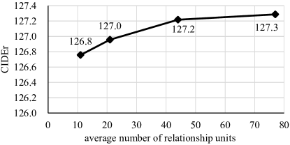
Figure 4. Results of training our model with different numbers of relationship units for images.

4.5. Qualitative Analysis

Visualization of Gating Weights.

To better understand the effect of our context gated fusion attention, we visualize the gating weights ($\boldsymbol{\beta}_{t}$ in Eqn. 17) of object, attribute, and relationship categories for each word in the generated captions in Figure 6. Our model successfully learns to attend to the category of VSUs that are consistent with the type of the current word, i.e. object, attribute, or relationship. For example, for the verbs like “laying”, the weights for the relationship category are generally the highest. The same observations could be found for the adjectives like “black” and “big”, and the nouns like “cat” and “clock”.

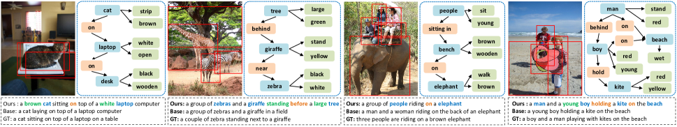
Figure 5. Example results of the generated captions (by our model, Up-Down baseline, and ground truth) and semantic graphs. Objects, attributes, and relationships are colored with blue, green, and orange, respectively.

Example Results.

Figure 5 shows four examples of the generated captions and semantic graphs for the images, where “ours”, “base”, “GT” denotes captions from our $\mathcal{G}^{S}+gate$ model, the Up-Down baseline, and the ground-truth, respectively. Generally, our model can generate more descriptive captions than Up-Down by enriching the sentences with more precise recognition of objects, detailed description of attributes, and comprehensive understanding of interactions between objects. For instance, in the second image, our model generates “standing before a large tree”, depicting the image content more comprehensively, while the base model fails to recognize the tree and the interactions between the animals and the tree.

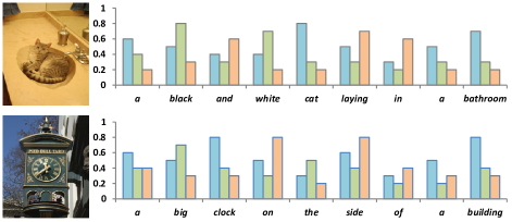
Figure 6. Visualization of the generated captions, and the per-word gating weights ($\boldsymbol{\beta}_{t}$) of them belonging to each of the three categories: object, attribute, and relationship.

5. Conclusion

We proposed to fill the information gap between visual content and linguistic description with visual semantic units (VSUs), which are visual components about objects, their attributes, and object-object interactions. We leverage structured graph (both semantic graph and geometry graph) to uniformly represent and GCNs to contextually embed the VSUs. A novel context gated attention module is introduced to hierarchically align words and VSUs. Extensive experiments on MS COCO have shown the superiority of our method.

References

- (1)
- Anderson et al. (2016) Peter Anderson, Basura Fernando, Mark Johnson, and Stephen Gould. 2016. SPICE: Semantic Propositional Image Caption Evaluation. (2016), 382–398.
- Anderson et al. (2017) Peter Anderson, Xiaodong He, Chris Buehler, Damien Teney, Mark Johnson, Stephen Gould, and Lei Zhang. 2017. Bottom-up and top-down attention for image captioning and vqa. arXiv preprint arXiv:1707.07998 (2017).
- Bastings et al. (2017) Joost Bastings, Ivan Titov, Wilker Aziz, Diego Marcheggiani, and Khalil Sima’an. 2017. Graph convolutional encoders for syntax-aware neural machine translation. arXiv preprint arXiv:1704.04675 (2017).
- Chen et al. (2018) Xinlei Chen, Li-Jia Li, Li Fei-Fei, and Abhinav Gupta. 2018. Iterative visual reasoning beyond convolutions. In Proceedings of the IEEE Conference on Computer Vision and Pattern Recognition. 7239–7248.
- Fang et al. (2014) Hao Fang, Saurabh Gupta, Forrest Iandola, Rupesh K. Srivastava, Li Deng, Piotr Doll¨¢r, Jianfeng Gao, Xiaodong He, Margaret Mitchell, and John C. Platt. 2014. From captions to visual concepts and back. (2014), 1473–1482.
- Gilmer et al. (2017) Justin Gilmer, Samuel S Schoenholz, Patrick F Riley, Oriol Vinyals, and George E Dahl. 2017. Neural message passing for quantum chemistry. In Proceedings of the 34th International Conference on Machine Learning-Volume 70. JMLR. org, 1263–1272.
- Gu et al. (2017) Jiuxiang Gu, Jianfei Cai, Gang Wang, and Tsuhan Chen. 2017. Stack-captioning: Coarse-to-fine learning for image captioning. arXiv preprint arXiv:1709.03376 (2017).
- Guo et al. (2019) Longteng Guo, Jing Liu, Peng Yao, Jiangwei Li, and Hanqing Lu. 2019. MSCap: Multi-Style Image Captioning With Unpaired Stylized Text. In Proceedings of the IEEE Conference on Computer Vision and Pattern Recognition. 4204–4213.
- He et al. (2016) Kaiming He, Xiangyu Zhang, Shaoqing Ren, and Jian Sun. 2016. Deep Residual Learning for Image Recognition. computer vision and pattern recognition (2016), 770–778.
- Hochreiter and Schmidhuber (1997) Sepp Hochreiter and Jürgen Schmidhuber. 1997. Long short-term memory. Neural computation 9, 8 (1997), 1735–1780.
- Johnson et al. (2015) Justin Johnson, Ranjay Krishna, Michael Stark, Li-Jia Li, David Shamma, Michael Bernstein, and Li Fei-Fei. 2015. Image retrieval using scene graphs. In Proceedings of the IEEE conference on computer vision and pattern recognition. 3668–3678.
- Karpathy and Feifei (2015) Andrej Karpathy and Li Feifei. 2015. Deep visual-semantic alignments for generating image descriptions. computer vision and pattern recognition (2015), 3128–3137.
- Kingma and Ba (2014) Diederik Kingma and Jimmy Ba. 2014. Adam: A method for stochastic optimization. arXiv preprint arXiv:1412.6980 (2014).
- Kipf and Welling (2016) Thomas N Kipf and Max Welling. 2016. Semi-supervised classification with graph convolutional networks. arXiv preprint arXiv:1609.02907 (2016).
- Krishna et al. (2017) Ranjay Krishna, Yuke Zhu, Oliver Groth, Justin Johnson, Kenji Hata, Joshua Kravitz, Stephanie Chen, Yannis Kalantidis, Li-Jia Li, David A Shamma, et al. 2017. Visual genome: Connecting language and vision using crowdsourced dense image annotations. International Journal of Computer Vision 123, 1 (2017), 32–73.
- Lin et al. (2014) Tsungyi Lin, Michael Maire, Serge J Belongie, James Hays, Pietro Perona, Deva Ramanan, Piotr Dollar, and C Lawrence Zitnick. 2014. Microsoft COCO: Common Objects in Context. european conference on computer vision (2014), 740–755.
- Liu et al. (2018) Daqing Liu, Zheng-Jun Zha, Hanwang Zhang, Yongdong Zhang, and Feng Wu. 2018. Context-Aware Visual Policy Network for Sequence-Level Image Captioning. In 2018 ACM Multimedia Conference on Multimedia Conference. ACM, 1416–1424.
- Lu et al. (2017) Jiasen Lu, Caiming Xiong, Devi Parikh, and Richard Socher. 2017. Knowing when to look: Adaptive attention via a visual sentinel for image captioning. In Proceedings of the IEEE Conference on Computer Vision and Pattern Recognition (CVPR), Vol. 6.
- Luo et al. (2018) Ruotian Luo, Brian Price, Scott Cohen, and Gregory Shakhnarovich. 2018. Discriminability objective for training descriptive captions. In Proceedings of the IEEE Conference on Computer Vision and Pattern Recognition. 6964–6974.
- Nagaraja et al. (2016) Varun K Nagaraja, Vlad I Morariu, and Larry S Davis. 2016. Modeling context between objects for referring expression understanding. In European Conference on Computer Vision. Springer, 792–807.
- Ren et al. (2015) Shaoqing Ren, Kaiming He, Ross Girshick, and Jian Sun. 2015. Faster r-cnn: Towards real-time object detection with region proposal networks. In Advances in neural information processing systems. 91–99.
- Rennie et al. (2017) Steven J Rennie, Etienne Marcheret, Youssef Mroueh, Jarret Ross, and Vaibhava Goel. 2017. Self-critical Sequence Training for Image Captioning. computer vision and pattern recognition (2017).
- Teney et al. (2017) Damien Teney, Lingqiao Liu, and Anton van den Hengel. 2017. Graph-structured representations for visual question answering. In Proceedings of the IEEE Conference on Computer Vision and Pattern Recognition. 1–9.
- Vinyals et al. (2015) Oriol Vinyals, Alexander Toshev, Samy Bengio, and Dumitru Erhan. 2015. Show and tell: A neural image caption generator. In Computer Vision and Pattern Recognition (CVPR), 2015 IEEE Conference on. IEEE, 3156–3164.
- Vinyals et al. (2017) Oriol Vinyals, Alexander Toshev, Samy Bengio, and Dumitru Erhan. 2017. Show and tell: Lessons learned from the 2015 mscoco image captioning challenge. IEEE transactions on pattern analysis and machine intelligence 39, 4 (2017), 652–663.
- Xu et al. (2017) Danfei Xu, Yuke Zhu, Christopher B Choy, and Li Fei-Fei. 2017. Scene graph generation by iterative message passing. In Proceedings of the IEEE Conference on Computer Vision and Pattern Recognition. 5410–5419.
- Xu et al. (2015) Kelvin Xu, Jimmy Lei Ba, Ryan Kiros, Kyunghyun Cho, Aaron C Courville, Ruslan Salakhudinov, Rich Zemel, and Yoshua Bengio. 2015. Show, Attend and Tell: Neural Image Caption Generation with Visual Attention. international conference on machine learning (2015), 2048–2057.
- Yang et al. (2018) Jianwei Yang, Jiasen Lu, Stefan Lee, Dhruv Batra, and Devi Parikh. 2018. Graph r-cnn for scene graph generation. In Proceedings of the European Conference on Computer Vision (ECCV). 670–685.
- Yang et al. (2019) Xu Yang, Kaihua Tang, Hanwang Zhang, and Jianfei Cai. 2019. Auto-encoding scene graphs for image captioning. In Proceedings of the IEEE Conference on Computer Vision and Pattern Recognition. 10685–10694.
- Yang et al. (2016) Zhilin Yang, Ye Yuan, Yuexin Wu, Ruslan Salakhutdinov, and William W Cohen. 2016. Review Networks for Caption Generation. (2016).
- Yao et al. (2018) Ting Yao, Yingwei Pan, Yehao Li, and Tao Mei. 2018. Exploring visual relationship for image captioning. In Proceedings of the European Conference on Computer Vision (ECCV). 684–699.
- Yao et al. (2016) Ting Yao, Yingwei Pan, Yehao Li, Zhaofan Qiu, and Tao Mei. 2016. Boosting Image Captioning with Attributes. (2016).
- You et al. (2016) Quanzeng You, Hailin Jin, Zhaowen Wang, Chen Fang, and Jiebo Luo. 2016. Image Captioning with Semantic Attention. (2016), 4651–4659.
- Zellers et al. (2018) Rowan Zellers, Mark Yatskar, Sam Thomson, and Yejin Choi. 2018. Neural motifs: Scene graph parsing with global context. In Proceedings of the IEEE Conference on Computer Vision and Pattern Recognition. 5831–5840.