Engineering Negative Cycle Canceling for Wind Farm Cabling

Abstract

In a wind farm turbines convert wind energy into electrical energy. The generation of each turbine is transmitted, possibly via other turbines, to a substation that is connected to the power grid. On every possible interconnection there can be at most one of various different cable types. Each type comes with a cost per unit length and with a capacity. Designing a cost-minimal cable layout for a wind farm to feed all turbine production into the power grid is called the Wind Farm Cabling Problem (WCP).

We consider a formulation of WCP as a flow problem on a graph where the cost of a flow on an edge is modeled by a step function originating from the cable types. Recently, we presented a proof-of-concept for a negative cycle canceling-based algorithm for WCP [15]. We extend key steps of that heuristic and build a theoretical foundation that explains how this heuristic tackles the problems arising from the special structure of WCP.

A thorough experimental evaluation identifies the best setup of the algorithm and compares it to existing methods from the literature such as Mixed-integer Linear Programming () and Simulated Annealing (SA). The heuristic runs in a range of half a millisecond to approximately one and a half minutes on instances with up to 500 turbines. It provides solutions of similar quality compared to both competitors with running times of one hour and one day. When comparing the solution quality after a running time of two seconds, our algorithm outperforms the - and SA-approaches, which allows it to be applied in interactive wind farm planning.

1 Introduction

Wind energy becomes increasingly important to help reduce effects of climate change. As of 2017, $11.6\,\%$ of the total electricity demand in the European Union is covered by wind power [25]. Across the Atlantic, the state of New York aims at installing 2.4 GW of offshore wind energy capacity by 2030, which could cover the demand of 1.2 million homes [20].

In an offshore wind farm a set of turbines generate electrical energy. From offshore substations the energy is transmitted via sea cables to an onshore grid point. One of the biggest wind farms currently planned is Hornsea Project Three in the North Sea with up to 300 turbines and twelve substations [1]. To transport turbine production to the substations, a system of cables links turbines to substations (internal cabling) where multiple turbines may be connected in series. The designer of a wind farm has various cable types available, each of which with respective costs and thermal capacities. The latter restricts the amount of energy that can be transmitted through a cable. Planning a wind farm as a whole consists of various steps, including determining the locations for turbines and substations, layouting the connections from substations to the grid point, and designing the internal cabling. The planning process comes with a high level of complexity, which automated approaches struggle with [24]. Therefore, one might opt for decoupling the planning steps. We call the task of finding a cost-minimal internal cabling of a wind farm with given turbine and substation positions, as well as given turbine production and substation capacities, the Wind Farm Cabling Problem (WCP). This problem is strongly $\mathcal{NP}$-hard [14].

Due to the overall cost of a wind farm, using one day of computation time or more arguably is a reasonable way to approach WCP. Such computation times, however, are not appropriate for an interactive planning process: Imagine a wind farm planner uses a planning tool which allows altering turbine positions to explore their influence on possible cable layouts. In that case, computation times of at most several seconds are desirable.

1.1 Contribution and Outline

We extend our recent proof-of-concept, in which negative cycle canceling is applied to a formulation of WCP as a network flow problem (cf. Section 3) with a step cost function representing the cable types [15]. The idea of negative cycle canceling is to iteratively identify cycles in a graph in which the edges are associated with the costs of (or gains from) changing the flow. Normally, a cycle of negative total cost corresponds to a way to decrease the cost of a previously found flow. Due to the step cost function, however, not every negative cycle helps improve a solution to WCP. We explore this and other issues for negative cycle canceling that arise from the step cost function in the flow problem formulation for WCP. We present a modification of the Bellman-Ford algorithm [3, 9] and build a theoretical foundation that explains how the modified algorithm addresses the aforementioned issues, e. g., by being able to identify cycles that actually improve a solution. This modification works on a subgraph of the line graph (cf. page 3) of the input graph and can be implemented in the same asymptotic running time as the original Bellman-Ford algorithm.

We further extend that heuristic by identifying two key abstraction layers and applying different strategies in those layers. Using different initializations is hinted at in the section on future work in [15]. We follow this hint and design eight concrete initialization strategies. In another layer, we propose a total of eight so-called “delta strategies” that specify the order in which different values for flow changes are considered.

In [15] we compared the Negative Cycle Canceling (NCC) algorithm to a Mixed-integer Linear Program () using the solver Gurobi with one-hour running times on benchmark sets from the literature [18]. We extend this evaluation by identifying the best of our variants and by comparing its results to the results of experiments after running times of two seconds, one hour, and one day on the same benchmark sets. A running time of two seconds helps identify the usefulness of the NCC algorithm to an interactive planning process. The other running times stand for non-time-critical planning. We also compare the algorithm to an approach using Simulated Annealing [18] with different running times. The results show that our heuristic is very fast since it terminates on instances with up to 500 turbines in under 100 seconds. At two seconds our algorithm outperforms its competitors, making it feasible for interactive wind farm planning. Even with longer running times for the - and SA-approaches, our algorithm yields solutions to WCP of similar quality but in tens of seconds.

In Section 2 we review existing work on WCP and negative cycle canceling. In Section 3 we define WCP as a flow problem. We give theoretical insights on the difference to standard flow problems and present and analyze our Negative Cycle Canceling algorithm in Section 4. An extensive experimental evaluation of the algorithm is given in Section 5. We conclude with a short summary of the results and outline possible research directions (see Section 6).

2 Related Work

In one of the first works on WCP, a hierarchical decomposition of the problem was introduced [4]. The layers relate to well-known graph problems and heuristics for various settings are proposed. Since then, considerable effort has been put into solving variants of WCP. Exact solutions can be computed using Mixed-integer Linear Program () formulations including various degrees of technical constraints, e. g., line losses, component failures, and wind stochasticity [19]. However, sizes of wind farms that are solved to optimality in reasonable time are small. Metaheuristics such as Genetic Algorithms [26, 6] or Simulated Annealing [18] can provide good but not necessarily optimal solutions in relatively short computation times.

We applied negative cycle canceling to a suitable flow formulation for WCP [15], but there is still an extensive agenda of open questions such as investigating the effect of other cable types, a comparison to existing heuristics, and using the solution as warm start for a solver. Originally, negative cycle canceling is proposed in the context of minimum cost circulations when linear cost functions are considered [17]. The algorithm for the Minimum-Cost Flow Problem based on cycle canceling with strongly polynomial running time runs in $\mathcal{O}(nm(\log n)\min\{\log(nC),m\log n\})$ time on a network with $n$ vertices, $m$ edges, and maximum absolute value of costs $C$ [12]. The bound for the running time of this algorithm was later tightened to $\Theta(\min\{nm\log(nC),nm^{2}\})$ [22]. Negative cycle canceling has also been used for problems with non-linear cost functions. Among these are multicommodity flow problems with certain non-linear yet convex cost functions based on a queueing model [21] and the Capacity Expansion Problem for multicommodity flow networks with certain non-convex and non-smooth cost functions [7]. A classic algorithm for finding negative cycles is the Bellman-Ford algorithm [3, 9] with heuristic improvements [13, 11]. An experimental evaluation of these heuristics and other negative cycle detection algorithms is given in [5].

A step cost function similar to the one in WCP appears in a multicommodity flow problem, for which exact solutions can be obtained by a procedure based on Benders Decomposition [10]. However, this procedure is only evaluated on instances with up to 20 vertices and 37 edges and some running times exceed 13 hours. While our approach does not guarantee to solve WCP to optimality, our evaluation shows that the solution quality is very good compared to the with running times not exceeding 100 seconds on wind farms with up to 500 turbines.

3 Model

The model presented in this paper is based on an existing flow model for WCP [15]. We briefly recall the model. Given a wind farm, let $V_{T}$ and $V_{S}$ be the sets of turbines and substations, respectively. We define a vertex set $V$ of a graph by $V=V_{T}\cup V_{S}$. For any two vertices $u$ and $v$ that can be connected by a cable in the wind farm, we define exactly one directed edge $e=(u,v)$, where the direction is chosen arbitrarily. We obtain a directed graph $G=(V,E)$ with $V=V_{T}\cup V_{S}$ and $E\subseteq\left(V\times V\right)\setminus\left(V_{S}\times V_{S}\right)$ such that $(u,v)\in E$ implies $(v,u)\notin E$. There are no edges between any two substations since we consider the wind farm planning step in which all positions of turbines and substations, as well as the cabling from substations to the onshore grid point have been fixed. We assume that all turbines generate one unit of electricity. Note that our algorithm can be easily generalized to handle non-uniform integral generation. Substations have a capacity $\mathrm{cap}_{\mathrm{sub}}\colon V_{S}\to\mathbb{N}$ representing the maximum amount of turbine production they can handle and each edge has a length given by $\mathrm{len}\colon E\to\mathbb{R}_{\geq 0}$ representing the geographic distance between the endpoints of the edge.

A flow on $G$ is a function $f\colon E\to\mathbb{R}$ and for an edge $(u,v)$ with $f(u,v)>0$ (resp. $<0$), we say that $f(u,v)$ units of flow go from $u$ to $v$ (resp. $-f(u,v)$ units go from $v$ to $u$). For a flow $f$ and a vertex $u$ we define the net flow in $u$ by $f_{\mathrm{net}}(u)=\sum_{(w,u)\in E}f(w,u)-\sum_{(u,w)\in E}f(u,w)$. A flow $f$ is feasible if the conditions on flow conservation for both turbines (Equation 1) and substations (Equation 2) are satisfied and if there is no outflow from any substation  (Equations 3 and 4).

$$f_{\mathrm{net}}(u) =-1 \forall u\in V_{T},$$ (1)

$$f_{\mathrm{net}}(v) \leq\mathrm{cap}_{\mathrm{sub}}(v) \forall v\in V_{S},$$ (2)

$$f(u,v) \geq 0 \forall(u,v)\in E:v\in V_{S},$$ (3)

$$f(v,u) \leq 0 \forall(v,u)\in E:v\in V_{S}.$$ (4)

Let $c\colon\mathbb{R}_{\geq 0}\to\mathbb{R}_{\geq 0}\cup\{\infty\}$ be a non-decreasing, left-continuous step function with $c(0)=0$. This function represents the cable costs and $\sup\{x\in\mathbb{R}_{\geq 0}:c(x)<\infty\}$ is the maximum cable capacity, which we assume to be a natural number. Note that such a function is neither convex nor concave in general. The cost of a flow on a wind farm graph is then given by

$$\mathrm{cost}(f)=\sum_{e\in E}c\left(\lvert f(e)\rvert\right)\cdot\mathrm{len}(e).$$ (5)

The value of $c\left(\lvert f(e)\rvert\right)$ stands for the cost per unit length of the cheapest cable type with sufficient capacity to transmit $\lvert f(e)\rvert$ units of turbine production. With all that, WCP is the problem of finding a feasible flow $f$ on a given wind farm graph that minimizes the cost. There is an analogon to the linear-cost integer flow theorem (e. g. [2, Thm. 9.10]) that guarantees an optimal flow with integral values.

Lemma .

Suppose the cost function is discontinuous only at integers and there is a feasible flow. Then, there is a cost-minimal integral flow.

Proof.

Suppose $f$ is a (possibly non-integral) flow of minimum costs. We define another flow network on the same graph by setting the capacity $\mathrm{cap}(e)$ of every edge $e$ to $\lceil\lvert f(e)\rvert\rceil$. Each turbine requires a net flow of $-1$. We model the substation capacities by adding a new vertex $s$ and edges from all substations to $s$ with capacities equal to the substation capacities. The net flow shall be $0$ at all substations and $\lvert V_{T}\rvert$ at $s$. We further define zero costs for flows on all edges. By the integrality property of min-cost flow problems with linear cost functions (e. g., [2, Thm. 9.10]) there is a feasible integral flow $f^{\prime}$ in this network. Due to the construction of the flow network, $f^{\prime}$ satisfies the constraints in Equations 1 to 4.

Since the cost function $c$ is non-decreasing, it holds for all $e\in E$ that $c(x)\leq c(\lvert f(e)\rvert)$ for all $x\in[0,\lvert f(e)\rvert]$. Since $c$ is a left-continuous step function that is discontinuous only at integers, we also have $c(x)\leq c(\lvert f(e)\rvert)$ for all $x\in[\lvert f(e)\rvert,\mathrm{cap}(e)]$. It holds in particular that $c(\lvert f^{\prime}(e)\rvert)\leq c(\lvert f(e)\rvert)$. Thus, $\mathrm{cost}(f^{\prime})\leq\mathrm{cost}(f)$ and $f^{\prime}$ is optimal in the original network.

∎

4 Algorithm

Given a wind farm graph $G$ we define the residual graph $R$ of $G$ with vertices $V(R)$ and edges $E(R)$ by $V(R)=V(G)\cup\{s\}$ and $E(R)=\{e,\bar{e}:e\in E(G)\}\cup\{(v,s),(s,v):v\in V_{S}\}$  where $\bar{e}$ is the reverse of $e$. The new vertex $s$, the super substation, is a virtual substation without capacity, that is connected to all substations. The edges to and from $s$ are used to model the substation capacity constraints and to allow the production of one turbine to be reassigned to another substation.

For a given feasible flow $f$ in $G$ of finite cost and $\Delta\in\mathbb{N}$ we further define residual costs, which represent by how much the cost for the edge changes if the flow on the edge is increased by $\Delta$ (cf. Figure 1 (a) – (d) for an example). Note that for negative quantities of flow this implies that the absolute value of the flow may be reduced or even the direction of the flow on an edge may change. More formally, we define $\gamma\colon E(R)\to\mathbb{R}$ by $\gamma(e)=\big{(}\,c(\lvert f(e)+\Delta\rvert)-c(\lvert f(e)\rvert)\,\big{)}\cdot\mathrm{len}(e)$ for all $e\in E(R)$ that are neither incident to $s$ nor lead to a substation where we alias $f(\bar{e})=-f(e)$ for all $e\in E(G)$. By this definition the residual costs are infinite if $c(\lvert f(e)+\Delta\rvert)=\infty$, i. e., if the maximal capacity on $e$ is exceeded. For $u\in V_{S}$ and $v\in V_{T}$, we set $\gamma(u,v)=\infty$ whenever $f(v,u)<\Delta$ because sending $f(u,v)+\Delta$ units from $u$ to $v$ would otherwise imply that flow leaves a substation. On edges into $s$, we set $\gamma(u,s)=0$ if and only if $f(u,s)+\Delta\leq\mathrm{cap}_{\mathrm{sub}}(u)$ and $\gamma(u,s)=\infty$ otherwise. On edges leaving the super substation, we set $\gamma(s,u)=0$ if and only if $f(u,s)\geq\Delta$ and $\gamma(s,u)=\infty$ otherwise to prevent flow from leaving the substation.

In a nutshell, the Negative Cycle Canceling (NCC) algorithm (Algorithm 1) starts with an initial feasible flow and some value of $\Delta$, computes the residual costs, and looks for a negative cycle in the residual graph. If the algorithm finds a negative cycle, it cancels the cycle, i. e., it changes the flow by adding $\Delta$ units of flow on all (residual) edges of the cycle. Note that this may decrease the actual amount of flow on edges of $G$. Then this procedure is repeated with the new flow and some value of $\Delta$ which may but not need to differ from the previous one. If no negative cycle is found, a new value of $\Delta$ is chosen and new residual costs are computed. This loop is repeated until all sensible values of $\Delta$ have been considered for a single flow, which is then returned by the algorithm. This flow is of integer value, since the initial flow is designed to only have integer values and we solely consider natural values for $\Delta$. Without loss of generality we can restrict ourselves to integer flows according to Section 3, even though our algorithm does not necessarily find an optimal solution of WCP. One question we answer is to what extent the algorithm benefits from different initial flows and different orders in which the values of $\Delta$ are chosen. We present various initializations and orders for $\Delta$ in Sections 4.3 and 4.4.

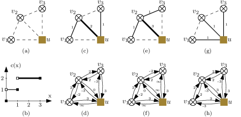
Figure 1: Examples of flows and corresponding residual graphs. (a) shows a wind farm graph. Edges between turbines are of length $2$, edges between the substation $u$ and any turbine are of length $3$. (b) depicts a cost function induced by two cable types. (c) displays a feasible flow. Dashed lines do not carry any flow. The thickness of solid lines represent the necessary cable type to carry the respective flow. (d) is the residual graph for the flow in (c) and $\Delta=1$. The super substation is omitted for ease of presentation. There are three negative cycles: $uv_{2}u$, $uv_{2}v_{1}u$, and $uv_{3}v_{2}u$. (e) shows the flow obtained by sending one unit of flow along $uv_{3}v_{2}u$ in (c). (f) is the residual graph for (e) and $\Delta=1$. (g) depicts the flow obtained by sending one unit of flow along $uv_{2}v_{1}u$ in (c). (h) displays the residual graph for (g) and $\Delta=1$.

The details of the algorithm (cf. Sections 4.1 and 4.2) address problems that arise from the special structure of WCP, namely the non-linear cost function $c$. Firstly, in classical min-cost flow problems, when $c$ is linear, the cost for changing flow by a certain amount is proportional to the amount of flow change (and the length of the respective edge) and does not depend on the current amount of flow on that edge. Hence, there is no need for computing residual costs for different values of $\Delta$. Secondly, short cycles, i. e., cycles of two edges, may have non-zero total cost in WCP (cf. cycle $uv_{2}u$ in Figure 1 (d)). Canceling such a cycle, however, does not change the flow and therefore does not improve the solution. Hence, only cycles of at least three edges (long cycles) are interesting to us because they do not contain both an edge and its reverse. Finding any negative cycle can be done in polynomial time but finding long negative cycles is $\mathcal{NP}$-hard for general directed graphs [16, Theorem 4 for $k=3$]. Thirdly, the order of canceling cycles matters (Figure 1 (c) – (g)). In (d), there are two long negative cycles: $uv_{2}v_{1}u$ and $uv_{3}v_{2}u$. After canceling $uv_{3}v_{2}u$ (Figure 1 (e)), the other cycle $uv_{2}v_{1}u$ is not negative anymore. Ultimately, Figure 1 (e) and (f) show that the non-existence of negative cycles in (all) residual graphs does not imply that the underlying flow is optimal—contrary to min-cost flow problems with linear cost functions. In other words, there are flows that represent local but not global minima.

4.1 Detecting Long Negative Cycles

We assume that the reader is familiar with the standard Bellman-Ford algorithm [3, 9], which is a common approach to finding negative cycles. We observed in preliminary experiments that it mostly reports short cycles even if long cycles exist. The reason is that negative residual costs on an edge are repeatedly used if the cost of the reverse edge is, say, zero. In that case, the negative residual cost strongly influences the distance labels on close vertices and overshadows long cycles (see cycle $uv_{2}u$ in comparison to cycle $uv_{2}v_{1}u$ in Figure 1 (d)).

One solution is to prohibit propagating the residual cost of an edge over its reverse edge. To this end, we employ the Bellman-Ford algorithm on the subgraph $L$ of the directed line graph of $R$ which we obtain from the line graph by removing all edges representing U-turns, i. e., edges of the form $(e,\bar{e})$ for $e\in E(R)$. We define the cost of an edge $(e_{1},e_{2})$ in $L$ as $\gamma(e_{2})$. At every vertex $e$ of $L$ we maintain a distance label $\mathrm{\ell}(e)$ initialized as $\gamma(e)$. Thus, throughout the Bellman-Ford algorithm, $\mathrm{\ell}(e)$ represents the length of some walk in $L$ starting at any vertex of $L$ and ending at $e$. By construction of $L$, the label $\mathrm{\ell}(e)$ also stands for some walk in $R$ which ends at the target vertex of $e$ and which does not traverse an edge of $R$ directly after its reverse. Consequently, a cycle $C$ in $L$ corresponds to a closed walk $W$ without U-turns of the same cost in $R$. In particular, $W$ is not a short cycle, which is what we wanted. It may still occur, however, that $W$ includes an edge and its reverse. In that case, $W$ consists of more than one cycle that may be negative themselves. Therefore, we decompose the closed walk $W$ into cycles, which, in turn, can be canceled one after another. For more details, refer to Section 4.2.

A downside of running the Bellman-Ford algorithm on the line graph is that more labels have to be stored and the running time of the algorithm is in $\mathcal{O}(\lvert V(L)\rvert\cdot\lvert E(L)\rvert)$, which is worse than the running time on $R$. We present how to implement an algorithm that directly works on $R$, that is equivalent to the Bellman-Ford algorithm on $L$, and that has the same asymptotic running time as the original Bellman-Ford algorithm on $R$. To this goal, we use the special structure of $L$ to analyze what the steps of the Bellman-Ford algorithm on $L$ mean for $R$. When running the Bellman-Ford algorithm on $L$, there is one label for every vertex of $L$. Each of those labels gives rise to a label on an edge of $R$. The labels at incoming edges of $v\in V(R)$ are used to compute the labels at outgoing edges of $v$. Let $(v,w)$ and $(v,x)$ be two edges leaving $v$. Let us assume that $(x,v)$ has the smallest label of all edges entering $v$. Then, $(x,v)$ is used to relax $(v,w)$. But it cannot be used to relax $(v,x)$. To do so, we need the second smallest label of all edges entering $v$. This yields the following observation.

Observation .

For each vertex $v$ of $R$ only the two smallest labels of incoming edges of $v$ are required to correctly update the labels on outgoing edges of $v$.

We call these labels relevant. Consequently, throughout our modified version of the Bellman-Ford algorithm, we maintain two distance labels $\mathrm{\ell}_{1}(v)$ and $\mathrm{\ell}_{2}(v)$, and two parent pointers $\mathrm{parent}_{1}(v)$ and $\mathrm{parent}_{2}(v)$ for every $v\in V(R)$, respectively. As above, $\mathrm{\ell}_{i}(v)$ with $i=1,2$ stand for the length of a U-turn-free walk whose first edge is arbitrary and whose last edge is $(\mathrm{parent}_{i}(v),v)$. That means that the parent pointers hold the edges that have been used to build the values of the distance labels. The algorithm ensures that $\mathrm{parent}_{1}(v)\neq\mathrm{parent}_{2}(v)$ and $\mathrm{\ell}_{1}(v)\leq\mathrm{\ell}_{2}(v)$ for every $v\in V(R)$. In every iteration of the Bellman-Ford algorithm, each edge of $R$ is considered for relaxation: For an edge $e=(u,v)$ take $\mathrm{\ell}(u)=\mathrm{\ell}_{1}(u)$ if $\mathrm{parent}_{1}(u)\neq v$ and $\mathrm{\ell}(u)=\mathrm{\ell}_{2}(u)$ otherwise. Then, check if $\mathrm{\ell}(u)+\gamma(e)$ yields a new relevant label at $v$. If, during a relaxation step, several incumbent labels and a newly computed candidate label have the same value, we break ties in favor of the older labels—as in the original algorithm. For each edge, checking if it yields a new relevant label at its end vertex can be done in constant time. With Section 4.1 we show reduced bounds for the number of iterations and the overall running time compared to a straightforward implementation on $L$.

Theorem .

If after $2\cdot\lvert V(R)\rvert$ iterations there is an edge that allows reducing a label, then there is a negative cycle in $L$.

Proof.

Let $n=\lvert V(R)\rvert$ and suppose $e_{2n+1}$ is an edge that allows reducing a label after $2n$ iterations. We iteratively construct a walk backwards starting from $e_{2n+1}$ by repeatedly applying the following procedure. At an edge $e_{i}=(v,w)$ we define $e_{i-1}$ as the incoming edge of $v$ other than $(w,v)$ with the smallest label. If there are several possibilities, we pick the edge with the oldest label among them. The label at $e_{i-1}$ is relevant by definition. We stop when an edge would be repeated. At this point, the walk contains a closed subwalk $W=(e_{k},\dots,e_{l})$ for suitable $k,l\in\mathbb{Z}$ with $k<l\leq 2n+1$. By Section 4.1 there are at most $2n$ edges with relevant labels. Hence $k\geq 1$.

Since the label at $e_{2n+1}$ can be updated after $2n$ iterations, the label at $e_{2n}$ must have been updated in iteration $2n$. Repeating this argument inductively shows that for $i\geq k$ the label at $e_{i}$ was updated in or after iteration $i$. Therefore, all labels of edges in $W$ were updated after the initialization. By the way the labels are computed, we therefore have

$$\mathrm{\ell}(e_{i-1})+\gamma(e_{i})\leq\mathrm{\ell}(e_{i})$$ (6)

for all edges $e_{i}$ on $W$ where we alias $e_{k-1}=e_{l}$.

If one of these inequalities is strict, i. e., $\mathrm{\ell}(e_{j-1})+\gamma(e_{j})<\mathrm{\ell}(e_{j})$ for some $j\in\{k,\dots,l\}$, then summing over the inequalities for all edges in $W$ will give

$$\sum_{e\in W}\big{(}\mathrm{\ell}(e)+\gamma(e)\big{)}<\sum_{e\in W}\mathrm{\ell}(e),$$ (7)

which can be simplified to

$$\sum_{e\in W}\gamma(e)<0.$$ (8)

Hence, the total costs of $W$ will be negative, which will complete the proof.

It remains to show that there is some edge $e_{j}=(v,w)$ for which the inequality is strict. To this aim let $e_{j}$ be the edge with the oldest label among edges in $W$. The label $\mathrm{\ell}(e_{j})$ was computed from the label $\mathrm{\ell}^{\prime}(e)$ of an edge $e=(u,v)$ with $u\neq w$, which may or may not be $e_{j-1}$. That means

$$\mathrm{\ell}^{\prime}(e)+\gamma(e_{j})=\mathrm{\ell}(e_{j})$$ (9)

where $\mathrm{\ell}$ denotes the labels after the algorithm finishes and $\mathrm{\ell}^{\prime}$ denotes the labels when $\mathrm{\ell}(e_{j})$ is computed. Note that the label at $e$ may have been updated afterwards, i. e., $\mathrm{\ell}(e)\leq\mathrm{\ell}^{\prime}(e)$.

For the sake of contradiction assume $\mathrm{\ell}(e_{j-1})\geq\mathrm{\ell}^{\prime}(e)$. Then,  $\mathrm{\ell}^{\prime}(e)\geq\mathrm{\ell}(e)\geq\mathrm{\ell}(e_{j-1})\geq\mathrm{\ell}^{\prime}(e)$ where the first inequality holds since labels at the same edge do not increase during the algorithm and the second inequality follows from $e$ being an incoming edge of $v$. Hence, all these labels are equal. The first equality implies that the label on $e$ was not updated after the point in time when $\mathrm{\ell}(e_{j})$ was computed and that $\mathrm{\ell}(e)$ is older than $\mathrm{\ell}(e_{j})$. Using the second equality, we distinguish two cases: If $e=e_{j-1}$, then $\mathrm{\ell}(e_{j-1})$ is older than $\mathrm{\ell}(e_{j})$, which contradicts the choice of $e_{j}$. If $e\neq e_{j-1}$, then $e$ should have been included in $W$ instead of $e_{j-1}$. Thus, the assumption of $\mathrm{\ell}(e_{j-1})\geq\mathrm{\ell}^{\prime}(e)$ is wrong and it holds that $\mathrm{\ell}(e_{j-1})<\mathrm{\ell}^{\prime}(e)$. Combining this inequality and Equation 9 completes the proof.∎

Corollary .

A negative cycle in $L$ can be computed in $\mathcal{O}(\lvert V(R)\rvert\cdot\lvert E(R)\rvert)$ time if one exists.

4.2 Algorithm in Detail

The previously described Bellman-Ford algorithm on $L$ is encapsulated in Algorithm 1. We first compute some initial flow (line 1) using one of eight initialization strategies presented in Section 4.3. In line 1 we compute the residual graph $R$ using a given flow $f$ and a given $\Delta$ and run the modified Bellman-Ford algorithm (line 1). In the repeat-loop, we consider one edge after another and check in line 1 if it can be relaxed (again). In that case, we extract a walk $W$ in $R$ with negative costs leading to that edge by traversing parent pointers. However, canceling $W$ directly may not improve the costs of the flow as $W$ may still contain an edge and its reverse. We decompose $W$ into a set of simple cycles $\mathcal{C}$ in line 1 and cancel each cycle independently if it is long and has negative costs (lines 1 to 1). Note that even though $W$ has negative costs, it may happen that only short cycles in $\mathcal{C}$ have negative costs and all long cycles have non-negative costs. In this case we search for another negative cycle in $L$ (line 1).

If no negative cycle in the current graph $L$ is canceled, a new value for $\Delta$ is determined according to the delta strategy (cf. Section 4.4) in line 1 and new residual costs $\gamma$ are computed. Line 1 also checks if every possible value for $\Delta$ has been used after the last update of $f$ without improving the solution. If so, $f$ is returned.

Input: Graph $G$, costs $c$, edge lengths $\mathrm{len}$

Result: A feasible flow $f$ in $G$

1 $f:=\textnormal{{InitializeFlow}}(G,\mathrm{len})$, $\Delta:=\textnormal{{InitialDelta}}$

2 while $\Delta\neq NULL$  do

3       $(R,\gamma):=\textnormal{{ComputeResidualGraph}}(G,c,f,\Delta)$

4       $\textnormal{{RunBellmanFord}}(R,\gamma)$

5       $\textnormal{{found}}:=\textnormal{{false}}$

6       foreach $e\in E(R)$ do

7             $W:=\textnormal{{FindNegativeClosedWalk}}(R,e)$

8             $\mathcal{C}:=\textnormal{{DecomposeWalkIntoCycles}}(W)$

9             foreach $C\in\mathcal{C}$  do

10                   if $\lvert C\rvert\geq 3$ and $\gamma(C)<0$  then

11                         $f:=\textnormal{{AddFlowOnCycle}}(f,C,\Delta)$

12                         $\textnormal{{found}}:=\textnormal{{true}}$

13                        

14                  

15            if found then break

16            

17      $\Delta:=\textnormal{{NextDelta}}(\Delta,\textnormal{{found}})$

18      

19return $f$

Algorithm 1 Negative Cycle Canceling

We apply two well-known speed-up techniques to the Bellman-Ford algorithm. Firstly, if one iteration does not yield any update of any label, then the computation is aborted and no negative cycle can be found in the current residual graph. Secondly, after sorting edges by start vertices, we track whether the labels at a vertex $v$ have been updated since last considering its outgoing edges. If not, then there is no need to relax the outgoing edges.

4.3 Initialization Strategies

Before we can start searching for and canceling negative cycles, we need some feasible initial flow. To obtain such a flow, we consider eight strategies, which all roughly work as follows. We pick a turbine $u$ whose production has not been routed to a substation yet. We then search for a shortest path $P$ from $u$ to a substation $v$ with free capacity using Dijkstra’s algorithm [8]. The search only considers edges on which the production of the turbine can be routed, i. e., it ignores congested edges. We then route the production of $u$ along $P$ to $v$.

We consider two metrics to compute shortest paths. Either we use the lengths defined by $\mathrm{len}$ (cf. Section 3) or we assume a length of $1$ for every edge. Turbine production can either be routed to a nearest or a farthest (in the sense of the respective metric) substation with free capacity. There are two ways in which the flow is updated: The simpler variant routes only the production of $u$ along $P$, i. e., the flow along $P$ is increased by $1$. The other variant greedily collects as much production from $u$ and other turbines on $P$ as possible without violating any capacity constraints. The resulting flows are integral since the substation capacities and the maximum cable capacity are natural numbers. If no feasible flow of finite cost is found during the initialization, the algorithm returns without a result.

This yields eight initialization strategies, which we name as follows. The base part of each name is either BFS if unit distances are used or Dijkstra (abbr. Dijk) if the distances given by $\mathrm{len}$ are used. This part is followed by a suffix specifying the target substation: Any (abbr. A) for the nearest and Last (abbr. L) for the farthest substation. An optional prefix of Collecting (abbr. C) means that the production is greedily collected along shortest paths. For example, CollectingDijkstraLast (abbr. C-Dijk-L) iterates over all turbines and for each turbine $u$ it finds the substation $v$ such that the shortest path given by $\mathrm{len}$ from $u$ to $v$ is longest among all substations. Along a shortest path from $u$ to $v$, turbine production is collected greedily.

4.4 Delta Strategies

A delta strategy consists of two parts: an initial value for $\Delta$ and a function that returns the value of $\Delta$ for the following iteration. We discuss eight delta strategies. The simplest one starts with $\Delta=1$ and increments $\Delta$ until a negative cycle is canceled. Then, $\Delta$ is reset to $1$. We call this strategy Inc (as in increasing). Similarly, Dec (as in decreasing) starts with the largest possible value for $\Delta$, which is twice the largest cable capacity. Then, $\Delta$ is decremented until a cycle is canceled and reset to the largest value. The third strategy IncDec behaves like Inc until a negative cycle is canceled. Then, it decrements $\Delta$ until $\Delta=1$ and behaves like Inc again. To improve performance, all $\Delta$ can be skipped during incrementation up to the last value of $\Delta$ for which a negative cycle was canceled. The fourth strategy Random returns random natural numbers between one and the maximum possible value for $\Delta$. Between any two cycle cancellations, no value is repeated.

For each strategy, we consider the following modification: After canceling a negative cycle, we retain the current value of $\Delta$, recompute the residual costs with the new flow, and run the Bellman-Ford algorithm again. We repeat this, until $\Delta$ does not yield a negative cycle. In that case, $\Delta$ is changed according to the respective delta strategy. We call the strategies after the modification StayInc, StayDec, StayIncDec, and StayRandom (or S-Inc, S-Dec, S-IncDec, and S-Random for short).

5 Experimental Evaluation

In the previous sections, we introduced a heuristic with various strategies for the WCP. We first use statistical tests to evaluate these strategies and identify the best ones (Section 5.1). Using the result we compare the best variant (i. e., best combination of initialization and delta strategy) with different base line algorithms for the WCP namely solving an exact formulation (Section 5.3) and a Simulated Annealing algorithm [18] (Section 5.4). In preliminary experiments (Section 5.2) we determine which of the solvers Gurobi and CPLEX works better for WCP to establish which solver we compare the NCC algorithm to.

For our evaluation we use benchmark sets for wind farms from the literature [18] consisting of wind farms of different sizes and characteristics: small wind farms with exactly one substation ($\mathcal{N}_{1}$: 10–79 turbines), wind farms with multiple substations ($\mathcal{N}_{2}$: 20–79 turbines, $\mathcal{N}_{3}$: 80–180 turbines, $\mathcal{N}_{4}$: 200–499 turbines), and complete graphs ($\mathcal{N}_{5}$: 80–180 turbines). Our code is written in C++14 and compiled with GCC $7.3.1$ using the -O3 -march=native flags. All simulations are run on a 64-bit architecture with four 12-core CPUs of AMD clocked at $2.1$ GHz with $256$ GB RAM running OpenSUSE Leap $15.0$. All computations are run in single-threaded mode to ensure comparability of the different algorithms.

5.1 Comparing Variants of our Algorithm

In a first step, we want to determine which delta strategy works best. To this end, we randomly select 200 instances per benchmark set. We run our algorithm on each instance with every pair of delta and initialization strategy. The first eight rows of Table 3 show for every benchmark set the minimum, average, and maximum running times for each delta strategy across all initialization strategies. We first observe that all variants are fast, with running times between tenths of milliseconds to $4.5$ minutes on large instances in the worst case. We see that Dec is always the slowest strategy on average, which can be explained by the fact that Dec often tries large values for $\Delta$, for which negative cycles are found rarely. The other strategies all roughly complete in the same time on average. It seems to be slightly faster to repeat the same $\Delta$. However, for our purpose all variants have small enough running times. We therefore base our decision, which variant to choose, solely on their solution qualities.

Table 1: Minimum, average and maximum of running times in milliseconds of different variants. Running time measurement starts before the initial flow is computed and ends with the termination of the algorithm prior to outputting the solution. The first eight rows represent running times across all initialization strategies per delta strategies and benchmark sets. The best delta strategy in terms of solution quality is marked in green; minimal values per column are marked in yellow. The last row represents the algorithm variant IncDec, CollectingDijkstraAny.

Delta Strategy

$\mathcal{N}_{1}$

$\mathcal{N}_{2}$

$\mathcal{N}_{3}$

$\mathcal{N}_{4}$

$\mathcal{N}_{5}$

$\min$

$\operatorname*{avg}$

$\max$

$\min$

$\operatorname*{avg}$

$\max$

$\min$

$\operatorname*{avg}$

$\max$

$\min$

$\operatorname*{avg}$

$\max$

$\min$

$\operatorname*{avg}$

$\max$

Dec

1.10

81.1

535

5.25

142.1

857

282

1.8k

11.3k

4.4k

59.7k

272k

2.4k

30.8k

216k

Inc

0.45

46.2

361

2.69

78.0

531

174

1.2k

8.4k

3.0k

49.1k

213k

1.8k

16.2k

131k

IncDec

0.45

45.9

433

2.67

77.7

539

174

1.2k

8.2k

3.0k

48.7k

212k

1.9k

16.2k

117k

Random

0.62

43.9

288

3.50

77.3

443

176

990

5.9k

3.2k

32.6k

137k

1.9k

16.6k

143k

S-Dec

0.76

62.2

461

3.76

111.4

725

210

1.4k

9.1k

3.5k

47.4k

206k

1.9k

14.7k

133k

S-Inc

0.46

42.2

295

2.70

72.8

438

171

1.0k

6.6k

2.8k

36.2k

147k

1.8k

14.4k

97k

S-IncDec

0.45

42.2

310

2.68

72.7

437

171

1.0k

6.3k

2.8k

36.0k

154k

1.8k

14.4k

120k

S-Random

0.57

44.1

333

3.25

79.1

486

193

1.1k

6.0k

3.0k

35.1k

147k

1.7k

14.1k

106k

BestVar

0.48

36.2

217

3.51

52.6

257

174

706

3.1k

3.0k

27.0k

92.6k

1.9k

13.4k

82.6k

Table 2: Comparison of delta strategies over all initialization strategies. An entry in row $i$ and column $j$ shows on how many instances strategy $i$ produces better solutions than strategy $j$. Values are marked by a star if they are significant with $p<10^{-2}$ and by two stars if $p<10^{-4}$. The best strategy is marked in green.

	Inc	Dec	IncDec	Random	S-Inc	S-Dec	S-IncDec	S-Random
Inc	—	$60.6\,\%^{\star\star}$	$48.4\,\%$	$60.2\,\%^{\star\star}$	$54.2\,\%$	$59.4\,\%^{\star\star}$	$50.7\,\%$	$56.5\,\%^{\star}$
Dec	$39.4\,\%$	—	$38.9\,\%$	$46.7\,\%$	$40.8\,\%$	$48.4\,\%$	$40.6\,\%$	$41.2\,\%$
IncDec	$51.6\,\%$	$61.1\,\%^{\star\star}$	—	$59.9\,\%^{\star\star}$	$54.0\,\%$	$60.1\,\%^{\star\star}$	$50.8\,\%$	$57.3\,\%^{\star}$
Random	$39.8\,\%$	$53.3\,\%$	$40.1\,\%$	—	$42.4\,\%$	$52\,\%$	$42.7\,\%$	$43.4\,\%$
S-Inc	$45.8\,\%$	$59.2\,\%^{\star\star}$	$46.0\,\%$	$57.6\,\%^{\star}$	—	$58.1\,\%^{\star\star}$	$46.9\,\%$	$54.7\,\%$
S-Dec	$40.6\,\%$	$51.6\,\%$	$39.9\,\%$	$48.0\,\%$	$41.9\,\%$	—	$41.7\,\%$	$41.9\,\%$
S-IncDec	$49.3\,\%$	$59.4\,\%^{\star\star}$	$49.2\,\%$	$57.3\,\%^{\star}$	$53.1\,\%$	$58.3\,\%^{\star\star}$	—	$55.4\,\%$
S-Random	$43.5\,\%$	$58.8\,\%^{\star\star}$	$42.7\,\%$	$56.6\,\%^{\star}$	$45.3\,\%$	$58.1\,\%^{\star\star}$	$44.6\,\%$	—

Table 3: Comparison of the initialization strategies when the delta strategy IncDec is fixed. An entry in row $i$ and column $j$ shows on how many instances strategy $i$ produces better solutions than strategy $j$. Values are marked by a star if they are significant with $p<10^{-2}$ and by two stars if $p<10^{-4}$. The best strategy is marked in green.

	Dijk-A	BFS-A	C-Dijk-A	C-BFS-A	Dijk-L	BFS-L	C-Dijk-L	C-BFS-L
Dijk-A	—	$55.8\,\%$	$49.5\,\%$	$54.9\,\%$	$55.6\,\%$	$53.7\,\%$	$53.9\,\%$	$56.5\,\%^{\star}$
BFS-A	$44.2\,\%$	—	$42.7\,\%$	$46.5\,\%$	$47.6\,\%$	$51.1\,\%$	$46.7\,\%$	$49.3\,\%$
C-Dijk-A	$50.5\,\%$	$57.3\,\%^{\star}$	—	$55.3\,\%$	$56.5\,\%$	$56.5\,\%^{\star}$	$54.4\,\%$	$56.3\,\%$
C-BFS-A	$45.1\,\%$	$53.5\,\%$	$44.7\,\%$	—	$51.2\,\%$	$54.5\,\%$	$49.3\,\%$	$55.4\,\%$
Dijk-L	$44.4\,\%$	$52.4\,\%$	$43.5\,\%$	$48.8\,\%$	—	$50.4\,\%$	$48.1\,\%$	$51.7\,\%$
BFS-L	$46.3\,\%$	$48.9\,\%$	$43.5\,\%$	$45.5\,\%$	$49.6\,\%$	—	$47.7\,\%$	$53.7\,\%$
C-Dijk-L	$46.1\,\%$	$53.3\,\%$	$45.6\,\%$	$50.7\,\%$	$51.9\,\%$	$52.3\,\%$	—	$53.1\,\%$
C-BFS-L	$43.5\,\%$	$50.7\,\%$	$43.7\,\%$	$44.6\,\%$	$48.3\,\%$	$46.3\,\%$	$46.9\,\%$	—

To compare the variants in terms of solution quality, we compute for each delta strategy $i$ and instance $m$ the mean $X^{(i)}_{m}$ of the solution values over all eight initialization strategies. This gives us 1000 data points per delta strategy. For delta strategies $i,j$ we perform a Binomial Sign Test counting instances with $X^{(i)}_{m}<X^{(j)}_{m}$ and $X^{(j)}_{m}<X^{(i)}_{m}$ (Appendix A), that means for this test we are rather interested in whether strategy $i$ performs better than strategy $j$ on instance $m$ and not by how much $i$ is better than $j$ on $m$. Table 3 summarizes the results of all tests after Bonferroni-correction by 112 (the number of tests from both delta and initialization strategies). The percentage given in an entry in row $i$ and column $j$ states on how many instances $i$ performes strictly better than $j$ after averaging over all initialization strategies. Note that entries $(i,j)$ and $(j,i)$ need not represent 1000 instances, as two variants may return equal solution values.

In the row IncDec, all values are above $50\,\%$, three of which are significant at the $10^{-4}$ and another one at the $10^{-2}$-level. The smallest value ($50.8\,\%$ in column StayIncDec) stands for 460 instances on which IncDec performs better than StayIncDec. To the contrary, there are 446 instances on which StayIncDec yields better solutions (cf. entry $49.2\,\%$ in row StayIncDec and column IncDec). While the differences between the four delta strategies involving Inc and IncDec are not statistically significant, IncDec does seem to have a slight advantage over the others. Hence we consider IncDec as the best delta strategy.

In Figure 2 (left), for the dark green curve all instances are ordered by $X^{(\texttt{Random})}_{m}/X^{(\texttt{IncDec})}_{m}$ in ascending order. For a given value $\alpha$ on the abscissa, the curve shows the relative cost factor of the instance at the $\alpha$-quantile in the computed order. The other curves work accordingly. We see, for example, that IncDec works strictly better than StayInc on $49.6\,\%$ and equally on $8.1\,\%$ of all instances and on $4.5\,\%$ of all instances IncDec outperforms Inc by at least $0.5\,\%$ in cost ratio. The minimum ratios range between 0.870 (Random) and 0.947 (Inc) and the maximum ratios are between 1.027 (Random) and 1.104 (StayIncDec).

Next, we want to find the best initialization strategy after fixing IncDec as the delta strategy. We pair each initialization strategy with IncDec on the same 1000 instances and summarize the results of all pairwise tests after Bonferroni-correction with factor 112 in Table 3. We see that both initialization strategies using Euclidean distances and routing turbine production to the nearest free substation, i. e., DijkstraAny and CollectingDijkstraAny, seem to work best. In particular, these are the only initialization strategies that show some significant advantage over other strategies. In Figure 2 (right) we depict ratios of solution values compared to CollectingDijkstraAny. The minimum ratios are between 0.886 and 0.923 for all strategies other than DijkstraAny (0.974). The maximum ratios range between 1.054 and 1.085. For the main part there is hardly any difference between collecting strategies and their non-collecting counterparts. The figure shows, e. g., that on roughly $22\,\%$ of all instances CollectingDijkstraAny is better than BFSAny and CollectingBFSAny by $0.5\,\%$. CollectingDijkstraAny has a slight but not significant advantage over DijkstraAny. We therefore declare CollectingDijkstraAny paired with IncDec as our best variant.

Figure 2: Evaluation of the NCC Algorithm using different strategies. For each strategy and for each instance, the ratio of the best solution value found by that NCC variant to the best solution value found by the reference variant (marked in red) are computed. They are shown in increasing order. The dashed lines represent the 25% and 75% quantiles of the instances. Left: The delta strategies are presented relative to the IncDec strategy. Solution values represent the average over all initialization strategies. Right: The initialization strategies are presented relative to the CollectingDijkstraAny strategy with fixed delta strategy IncDec.

The last row in Table 3 shows the running time characteristics of CollectingDijkstraAny paired with IncDec. Running times range between tenths of milliseconds and 100 seconds.

5.2 Comparing solvers to establish baseline solver

We conduct preliminary experiments to determine which solver we use as a baseline for our algorithm. To this goal, we randomly choose 35 instances each from benchmark sets $\mathcal{N}_{1}$, and $\mathcal{N}_{2}$ and 70 instances each from benchmark sets $\mathcal{N}_{3}$, $\mathcal{N}_{4}$, and $\mathcal{N}_{5}$. We compare Gurobi 8.0.0 and IBM ILOG CPLEX Optimization Studio v12.8 with a running time of one day per instance and solver using the formulation from Appendix B. Since computing an optimal solution to the takes too long in almost all instances, we restrict the solvers to different maximum running times. Each solver uses one thread per instance and node files are written to disk after the solver uses more than 0.5 GB of memory to store node files. Other than that, default values are used.

During the experiments, we consider three time stamps: one hour, twelve hours, and one day. For each solver, instance, and time stamp we record the value of the best incumbent solution and the MIP gap. If a solver terminates with a proven optimal solution after time stamp $t$, then the respective values during termination are assigned to all subsequent time stamps.

The results of the experiment are depicted in Figure 3 for the quality of the best solution found by the respective solver and in Figure 4 for a comparison of MIP gaps. In Figure 3 each data point corresponds to an instance and a time stamp. The value on the abscissa stands for a normalized difference in solution values, i. e., $\nicefrac{{(\mathrm{sol}_{\mathrm{Gurobi}}-\mathrm{sol}_{\mathrm{CPLEX}})}}{{\max(\mathrm{sol}_{\mathrm{Gurobi}}\mkern-1.5mu,\,\mathrm{sol}_{\mathrm{CPLEX}})}}$. This yields a value in $[-1,1]$, which is negative if and only if Gurobi finds a better solution than CPLEX. Figure 4 shows the MIP gaps computed by CPLEX and Gurobi for each instance and time stamps. MIP gaps (or relative gaps) are a standard notion from Mixed-integer Linear Programming. The best feasible solution the solver finds yields an upper bound ($\mathrm{ub}$) on the optimal value. The solver also tries to prove lower bounds ($\mathrm{lb}$). Combining the best upper and the best lower bound yield the MIP gap $\nicefrac{{\mathrm{ub}-\mathrm{lb}}}{{\mathrm{ub}}}$. This value is in the unit interval and gives information on how “bad” the solution value can be compared to the (unknown) optimal value. A value of zero shows that the best feasible solution found by the solver is optimal. Note, however, that a solution might be optimal even though the gap is positive.

Figure 3: Comparison solution values found by solvers CPLEX and Gurobi after different running times. For each instance and running time the abscissa shows a normalized difference in solution values, i. e., $\nicefrac{{(\mathrm{sol}_{\mathrm{Gurobi}}-\mathrm{sol}_{\mathrm{CPLEX}})}}{{\max(\mathrm{sol}_{\mathrm{Gurobi}}\mkern-1.5mu,\,\mathrm{sol}_{\mathrm{CPLEX}})}}$. There are twelve instances from $\mathcal{N}_{5}$ with a value between -0.29 and -0.49 and another three instances from $\mathcal{N}_{5}$ with a value less than -0.99. Four instances from $\mathcal{N}_{5}$ are infeasible.

Figure 4: Comparison of gaps between solution values and lower bounds on the optimal value for solutions computed by CPLEX and Gurobi separated by benchmark sets after different maximum running times: Left: one hour, Middle: twelve hours, Right: one day.

Evidently, Gurobi performs better across all benchmark sets and time stamps. While there is evidence that the best incumbent solutions computed by Gurobi and CPLEX become more similar the longer the experiments run, we also see that Gurobi seems to work better than CPLEX the bigger the instances become. We therefore use Gurobi as the solver to compute the baseline to which we compare the negative cycle canceling-based algorithm.

5.3 Comparing our Best Variant with Gurobi

We compare our algorithm in its best variant, i. e., CollectingDijkstraAny with IncDec, with Gurobi on the formulation in Appendix B. We randomly select 200 instances per benchmark set from the benchmark sets in [18].

Figure 5: Comparison of the NCC algorithm to Gurobi on 200 instances per benchmark set. The ordinate shows the ratio of objective values at various maximum running times of our algorithm to objective values of Gurobi. Running times: Left: two seconds, Middle: one hour, Right: one day.

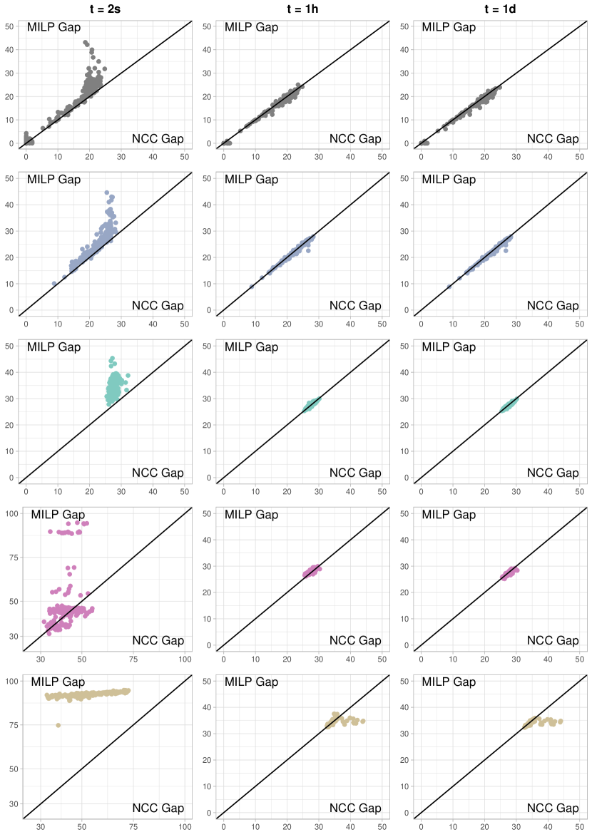
Figure 6: Comparison of gaps between solution values and lower bounds on the optimal value for solutions computed by Gurobi () and the NCC algorithm separated by benchmark sets ($\mathcal{N}_{1}$ in row 1 through $\mathcal{N}_{5}$ in row 5) after maximum running times of two seconds, one hour, and one day. Lower bounds are taken from experiments with running times of one day.

In Figure 5 we plot the ratio of the best solution value found by our algorithm to Gurobi’s best solution at running times of two seconds, one hour, and one day for each benchmark set separately. These running times represent both interactive and non-time-critical planning. Since our algorithm terminates in under 100 seconds, the comparisons in Figure 5 (middle and right) use the solution our algorithm provides at termination. While discussing the plots, we also discuss an adaptation of the relative gaps $\nicefrac{{\mathrm{ub}-\mathrm{lb}}}{{\mathrm{ub}}}$ we introduced in Section 5.2. For each instance, we use the lower bounds from the one-day experiments. For each instance, each maximum running time and for both the and the NCC algorithm take best solution value ($\mathrm{ub}$) found at the maximum running time. We refer to the relative gaps as gap and NCC gap, respectively, and show them in Figure 6.

After two seconds our algorithm outperforms Gurobi on all benchmark sets as it finds better solutions on $89\,\%$ of all instances with the lowest percentage on benchmark set $\mathcal{N}_{4}$. On $\mathcal{N}_{1}$ the NCC gaps are on average $14.1\,\%$ with a maximum of $24.8\,\%$ compared to gaps of $16.9\,\%$ on average and at most $43.1\,\%$. For $\mathcal{N}_{3}$, the NCC gaps are on average $27.6\,\%$ with a spread of only seven percentage points, compared to a mean of $34.6\,\%$ and a maximum of $45.4\,\%$ for the gap. The values for $\mathcal{N}_{2}$ range between those for $\mathcal{N}_{1}$ and $\mathcal{N}_{3}$. The ratios of solution values range between 0.699 and 1.019 for $\mathcal{N}_{1}$, $\mathcal{N}_{2}$, and $\mathcal{N}_{3}$. On $\mathcal{N}_{4}$, which contains the largest instances, our algorithm computes better solutions on $62\,\%$ of the instances. On six instances Gurobi does not find a solution. The instances on which Gurobi is better are on average larger than the other instances in $\mathcal{N}_{4}$. There are 18 instances on which the ratio of solution values exceeds 1.1 with a maximum of 1.228. On those very large instances, detecting negative cycles takes longer and fewer iterations are performed in two seconds. The NCC gaps spread between $31.6\,\%$ and $57.4\,\%$ with an average of $42.6\,\%$. The gaps are even worse with a mean value of $48.3\,\%$ and 18 instances above $88.5\,\%$. On the complete graphs of $\mathcal{N}_{5}$, our algorithm produces solutions that are at least $75\,\%$ cheaper than Gurobi’s on all but one instance (which has a ratio of 0.411). The gaps are on average at $53.6\,\%$ for the NCC algorithm and at $92.3\,\%$ for Gurobi.

Within one hour (middle plot in Figure 5) Gurobi finds better or equivalent solutions than our algorithm on a majority of the instances in benchmark sets $\mathcal{N}_{1}$, $\mathcal{N}_{2}$, and $\mathcal{N}_{3}$. On $25\,\%$ of the instances from $\mathcal{N}_{1}$, on $18.5\,\%$ of the instances from $\mathcal{N}_{2}$, and on one instance from $\mathcal{N}_{3}$ the solution values are equal. On $\mathcal{N}_{4}$ and $\mathcal{N}_{5}$, our algorithm still yields better solutions on $87.5\,\%$ and $52\,\%$ of the instances, respectively. Our algorithm is within $0.5\,\%$ of Gurobi’s best solution on $81.4\,\%$ and within $1\,\%$ on $91.3\,\%$ of all instances. Only on six of 1000 instances (all in $\mathcal{N}_{5}$), the ratio exceeds 1.10 with a maximum of 1.165. That means, while the NCC algorithm is comparable to Gurobi in solution quality on small instances, it proves better on larger wind farms. Furthermore, our algorithm is much faster since it terminates in under 100 seconds—compared to one hour of maximum running time for Gurobi.

After running times of one day (right plot in Figure 5), while our algorithm is at least as good as Gurobi only on between $25\,\%$ ($\mathcal{N}_{5}$) and $38.5\,\%$ ($\mathcal{N}_{1}$) of the instances, it is within $1\,\%$ of Gurobi’s solution on $87.7\,\%$ of all instances. Again, there are only six instances with a ratio worse than 1.10 with a maximum of 1.169. Our algorithm does not profit from long running times since it gets stuck in local minima. Thus, the solver is the better choice if more time is available. Between running times of one hour and one day, the gaps look vastly the same and there is hardly any difference between NCC gaps and gaps. They range between zero and $25.0\,\%$ on $\mathcal{N}_{1}$, clot around $28\,\%$ for $\mathcal{N}_{3}$ and  $\mathcal{N}_{4}$ and around $34\,\%$ for $\mathcal{N}_{5}$ with seven outliers to the worse by the NCC algorithm.

In summary, these experiments show that the NCC algorithm is a viable option compared to Gurobi with long running times and that it yields better solutions than the solver if only a short amount of time is given.

5.4 Comparison to Metaheuristic Simulated Annealing

Figure 7: Comparison of Negative Cycle Canceling algorithm to the Simulated Annealing algorithm on 200 instances per benchmark set. The ordinate represents the ratio of objective values at different maximum running times of our algorithm to objective values of the Simulated Annealing algorithm. Left: Running time of two seconds. Right: Running time of one hour.

We compare our best algorithm variant with the best variant of a Simulated Annealing (SA) algorithm [18]. We run the SA algorithm on 200 randomly selected instances per benchmark set (independently selected from other experiments). We compare the best solutions found after two seconds and one hour (Figure 7).

After two seconds, the NCC algorithm performs at least as good as the SA algorithm on all instances from $\mathcal{N}_{3}$ and on $74.5\,\%$ and $90.5\,\%$ on $\mathcal{N}_{1}$ and $\mathcal{N}_{2}$, respectively. The minimum ratios are 0.381 for $\mathcal{N}_{1}$, 0.911 for $\mathcal{N}_{2}$, and 0.875 for $\mathcal{N}_{3}$ with one instance in $\mathcal{N}_{2}$ where the SA algorithm does not find a solution. The maximum ratio on those benchmark sets is at most 1.034. On the larger instances of $\mathcal{N}_{4}$ and $\mathcal{N}_{5}$, our algorithm presumably cannot perform sufficient iterations, as the SA algorithm is better on $71\,\%$ of those instances. Yet, the SA algorithm does not find feasible solutions on $38.5\,\%$ of instances from $\mathcal{N}_{5}$. The ratios have a wide spread: from 0.203 to 1.261 for $\mathcal{N}_{4}$ and from 0.838 to 1.480 for $\mathcal{N}_{5}$ (save for the instances without a solution from the SA algorithm).

After one hour, the SA algorithm provides better solutions than our algorithm on $67.5\,\%$ and $80\,\%$ of instances from $\mathcal{N}_{2}$ and $\mathcal{N}_{3}$, respectively. Our algorithm, however, stays within $1\,\%$ in solution quality on $84.2\,\%$ on the benchmark sets $\mathcal{N}_{1}$–$\mathcal{N}_{3}$. Again, our algorithm seems to be stuck in local minima. On $\mathcal{N}_{4}$ and $\mathcal{N}_{5}$, our algorithm performs better than the SA algorithm on $86\,\%$ and $74.5\,\%$, respectively. Apparently, the SA algorithm needs more time to explore the solution space. The minimum ratios of solution values are as low as 0.716 for $\mathcal{N}_{1}$ and between 0.905 and 0.995 for the other benchmark sets. The maximum ratios are at most 1.057 for all benchmark sets except $\mathcal{N}_{5}$ (1.159). This supports our findings from the experiments that our algorithm is competitive to other approaches to solving WCP within very short amounts of time. In view of an interactive planning process, it stands out that the SA algorithm struggles to find solutions quickly in dense graphs.

6 Conclusion

Based on recently presented ideas [15] we propose and compare numerous variants of a Negative Cycle Canceling heuristic for the Wind Farm Cabling Problem. While all variants run in the order of milliseconds up to 4.5 minutes, they differ significantly in quality. We identify the best variant and use it to compare our heuristic to the solver Gurobi and a Simulated Annealing algorithm from the literature. With these comparisons we are able to solve several open questions [15]. While the solver Gurobi has the potential to find optimal solutions if it runs long enough, our heuristic is able to find solutions of comparable quality in only a fraction of the time. Our algorithm beats Gurobi in finding good solutions in a matter of seconds. We make similar observations when we compare ourselves to a Simulated Annealing approach.

Moving forward, one may investigate how to improve the solution quality of our heuristic. Visually comparing flows from our algorithm and other solution methods may help to identify what kind of more complex circulations improve the solution. It then remains to investigate how these circulations can be detected. Also, methods for escaping local minima such as temporarily allowing worse solutions could help to improve our algorithm. It also remains open whether one can prove any theoretical guarantees on the solution quality or the number of iterations. Along the same lines, any theoretical insights on why one delta or initialization strategy works better than another, or on the order in which cycles should be canceled could help improve the NCC algorithm.

In a broader algorithmic view, the heuristic can be easily generalized to minimum-cost flow problems with other types of cost functions provided that one searches for integral flows. It would be interesting to see how well the heuristic performs there.

Appendix A Binomial Sign Test for Two Dependent Samples

Statistical tests help to find the best strategy variant for our algorithm with regards to available initialization strategies (Section 4.3) and delta strategies (Section 4.4). In our case, we use the Binomial Sign Test for two dependent samples [23, p. 303].

We explain this test in a general setting here and specify how we apply the test in more detail below. Generally speaking, we compare $k$ variants of an algorithm. In our case these are the different initialization and delta strategies (Sections 4.3 and 4.4). We apply each variant to each instance. For every instance $m$, we denote the total cost of the resulting flow computed by variant $i$ on instance $m$ by $X^{(i)}_{m}$.

For any ordered pair of two variants $(i,j)$ running on a fixed instance $m$, we calculate its solution difference $D=X^{(i)}_{m}-X^{(j)}_{m}$ and increment—depending on the sign of $D$—either $D_{i<j},D_{i>j}$, or $D_{i=j}$ where, for example, $D_{i<j}$ counts the instances in which $i$ performed better than $j$. If both variants were equally good, then $D_{i<j}\sim\mathrm{Bin}(D_{i<j}+D_{i>j},0.5)$, i. e., $D_{i<j}$ is binomially distributed on $D_{i<j}+D_{i>j}$ trials and probability $0.5$.

We perform $k(k-1)$ tests, one for each ordered pair of variants, and always test the null hypothesis $\mathrm{H}_{0}\colon\theta=0.5$ against the alternative hypothesis $\mathrm{H}_{1}\colon\theta>0.5$ where $\theta$ is the probability in the underlying hypothesized distribution $D_{i<j}\sim\mathrm{Bin}(D_{i<j}+D_{i>j},\theta)$. The resulting $p$-values are Bonferroni-corrected by the number of tests. In this setting, we interpret rejecting $\mathrm{H}_{0}$ as algorithm variant $i$ performing better than algorithm variant $j$.

Appendix B formulation

Recall that we introduced the notion of cable types in Section 1. Let $K$ denote the set of cable types. Each cable type $k\in K$ has a capacity on the amount of turbine production that can be transmitted through it, which we denote by $\mathrm{cap}_{k}$, as well as a cost per unit length $c_{k}$ for laying a cable of type $k$. The formulation for WCP we used in our experiments is as follows:

$$\min \sum_{e\in E}\sum_{k\in K}c_{k}\cdot x(e,k)\cdot\mathrm{len}(e)$$ (10)

$$\text{s.\ t. }f_{\mathrm{net}}(u) =-1 \forall u\in V_{T},$$ (11)

$$f_{\mathrm{net}}(v) \leq\mathrm{cap}_{\mathrm{sub}}(v) \forall v\in V_{S},$$ (12)

$$\lvert f(e)\rvert \leq\sum_{k\in K}x(e,k)\cdot\mathrm{cap}_{k} \forall e\in E,$$ (13)

$$\sum_{k\in K}x(e,k) \leq 1 \forall e\in E,$$ (14)

$$f(u,v) \leq 0 \forall(u,v)\in E\colon u\in V_{S},$$ (15)

$$f(u,v) \geq 0 \forall(u,v)\in E\colon v\in V_{S},$$ (16)

where $f_{\mathrm{net}}$ denotes the net flow defined in Section 3, $f\in\mathbb{R}^{E}$, and $x\in\{0,1\}^{E\times K}$. Equations 11 and 12 are the same as the constraints given in Equations 1 and 2. Equation 13 ensures that there is enough cable capacity installed on every edge for the respective flow, while there is only one cable type on that edge due to Equation 14. Equations 15 and 16 correspond to Equations 3 and 4 and ensure that no flow leaves any substation.

References

- [1] 4C Offshore Ltd. Hornsea Project Three Offshore Wind Farm, 2018. www.4coffshore.com/windfarms/hornsea-project-three-united-kingdom-uk1k.html, Accessed: 2018-08-15.
- [2] Ravindra K. Ahuja, Thomas L. Magnanti, and James B. Orlin. Network flows: theory, algorithms, and applications. Prentice Hall, Upper Saddle River, NJ [u.a.], 1993.
- [3] Richard Bellman. On a routing problem. Quarterly of Applied Mathematics, 16:87–90, 1958. doi:10.1090/qam/102435.
- [4] Constantin Berzan, Kalyan Veeramachaneni, James McDermott, and Una-May O’Reilly. Algorithms for cable network design on large-scale wind farms. Technical report, Massachusetts Institute of Technology, 2011.
- [5] Boris V. Cherkassky and Andrew V. Goldberg. Negative-cycle detection algorithms. Mathematical Programming, 85(2):277–311, Jun 1999. doi:10.1007/s101070050058.
- [6] Ouahid Dahmani, Salvy Bourguet, Mohamed Machmoum, Patrick Guerin, Pauline Rhein, and Lionel Josse. Optimization of the connection topology of an offshore wind farm network. IEEE Systems Journal, 9(4):1519–1528, 2015. doi:10.1109/JSYST.2014.2330064.
- [7] Mauricio C. de Souza, Philippe Mahey, and Bernard Gendron. Cycle-based algorithms for multicommodity network flow problems with separable piecewise convex costs. Networks, 51(2):133–141, 2008. doi:10.1002/net.20208.
- [8] Edsger W. Dijkstra. A note on two problems in connexion with graphs. Numerische Mathematik, 1(1):269–271, Dec 1959. doi:10.1007/BF01386390.
- [9] Lester R. Ford, Jr. and Delbert R. Fulkerson. Flows in Networks. Princeton University Press, Princeton, NJ, USA, 2010.
- [10] Virginie Gabrel, Arnaud Knippel, and Michel Minoux. Exact solution of multicommodity network optimization problems with general step cost functions. Operations Research Letters, 25(1):15 – 23, 1999. doi:10.1016/S0167-6377(99)00020-6.
- [11] Andrew V. Goldberg and Tomasz Radzik. A heuristic improvement of the Bellman-Ford algorithm. Applied Mathematics Letters, 6(3):3 – 6, 1993. doi:10.1016/0893-9659(93)90022-F.
- [12] Andrew V. Goldberg and Robert E. Tarjan. Finding minimum-cost circulations by canceling negative cycles. Journal of the ACM, 36(4):873–886, October 1989. doi:10.1145/76359.76368.
- [13] Donald Goldfarb, Jianxiu Hao, and Sheng-Roan Kai. Shortest path algorithms using dynamic breadth-first search. Networks, 21(1):29–50, 1991. doi:10.1002/net.3230210105.
- [14] Sascha Gritzbach. Cable layout optimization problems in the context of renewable energy sources, 2023. doi:10.5445/IR/1000158746.
- [15] Sascha Gritzbach, Torsten Ueckerdt, Dorothea Wagner, Franziska Wegner, and Matthias Wolf. Towards negative cycle canceling in wind farm cable layout optimization. In Proceedings of the 7th DACH+ Conference on Energy Informatics, volume 1 (Suppl 1). Springer, 2018. doi:10.1186/s42162-018-0030-6.
- [16] Longkun Guo and Peng Li. On the complexity of detecting -length negative cost cycles. In Combinatorial Optimization and Applications, COCOA 2017, volume 10627 of Lecture Notes in Computer Science, pages 240–250. Springer International Publishing, 2017. doi:10.1007/978-3-319-71150-8_21.
- [17] Morton Klein. A primal method for minimal cost flows with applications to the assignment and transportation problems. Management Science, 14(3):205–220, 1967. doi:10.1287/mnsc.14.3.205.
- [18] Sebastian Lehmann, Ignaz Rutter, Dorothea Wagner, and Franziska Wegner. A simulated-annealing-based approach for wind farm cabling. In Proceedings of the Eighth International Conference on Future Energy Systems, e-Energy ’17, pages 203–215, New York, NY, USA, 2017. ACM. doi:10.1145/3077839.3077843.
- [19] Sara Lumbreras and Andres Ramos. Optimal design of the electrical layout of an offshore wind farm applying decomposition strategies. IEEE Transactions on Power Systems, 28(2):1434–1441, 2013. doi:10.1109/TPWRS.2012.2204906.
- [20] New York State Energy Research and Development Authority. New York State Offshore Wind Master Plan, 2017. https://www.nyserda.ny.gov/-/media/Files/Publications/Research/Biomass-Solar-Wind/Master-Plan/Offshore-Wind-Master-Plan.pdf, Accessed: 2018-08-15.
- [21] Adam Ouorou and Philippe Mahey. A minimum mean cycle cancelling method for nonlinear multicommodity flow problems. European Journal of Operational Research, 121(3):532 – 548, 2000. doi:10.1016/S0377-2217(99)00050-8.
- [22] Tomasz Radzik and Andrew V. Goldberg. Tight bounds on the number of minimum-mean cycle cancellations and related results. Algorithmica, 11(3):226–242, Mar 1994. doi:10.1007/BF01240734.
- [23] David J. Sheskin. Handbook of parametric and nonparametric statistical procedures. A Chapman & Hall Book. CRC Press, Taylor & Francis, Boca Raton [u.a.], 5. ed. edition, 2011.
- [24] Pedro Santos Valverde, António J. N. A. Sarmento, and Marco Alves. Offshore wind farm layout optimization – state of the art. Journal of Ocean and Wind Energy, 1(1):23–29, 2014.
- [25] WindEurope asbl/vzw. Wind in power 2017, 2018. https://windeurope.org/wp-content/uploads/files/about-wind/statistics/WindEurope-Annual-Statistics-2017.pdf, Accessed: 2018-08-15.
- [26] Menghua Zhao, Zhe Chen, and Frede Blaabjerg. Optimization of electrical system for a large DC offshore wind farm by genetic algorithm. In Proceedings of NORPIE 2004, pages 1–8, 2004.