The CANDELS/SHARDS multi-wavelength catalog in GOODS-N: Photometry, Photometric Redshifts, Stellar Masses, Emission line fluxes and Star Formation Rates

Abstract

We present a WFC3 F160W ($H$-band) selected catalog in the CANDELS/GOODS-N field containing photometry from the ultraviolet (UV) to the far-infrared (IR), photometric redshifts and stellar parameters derived from the analysis of the multi-wavelength data. The catalog contains 35,445 sources over the 171 arcmin² of the CANDELS F160W mosaic. The 5$\sigma$ detection limits (within an aperture of radius 0$\farcs$17) of the mosaic range between $H=27.8$, 28.2 and 28.7 in the wide, intermediate and deep regions, that span approximately 50%, 15% and 35% of the total area. The multi-wavelength photometry includes broad-band data from UV (U band from KPNO and LBC), optical (HST/ACS F435W, F606W, F775W, F814W, and F850LP), near-to-mid IR (HST/WFC3 F105W, F125W, F140W and F160W, Subaru/MOIRCS Ks, CFHT/Megacam K, and Spitzer/IRAC 3.6, 4.5, 5.8, 8.0 $\mu$m) and far IR (Spitzer/MIPS 24$\mu$m, HERSCHEL/PACS 100 and 160$\mu$m, SPIRE 250, 350 and 500$\mu$m) observations. In addition, the catalog also includes, optical medium-band data (R$\sim 50$) in 25 consecutive bands, $\lambda=500$ to 950 nm, from the SHARDS survey and WFC3 IR spectroscopic observations with the G102 and G141 grisms (R$\sim 210$ and 130). The use of higher spectral resolution data to estimate photometric redshifts provides very high, and nearly uniform, precision from $z=0-2.5$. The comparison to 1,485 good quality spectroscopic redshifts up to $z\sim 3$ yields $\Delta z$/(1+$z_{\rm spec}$)$=$0.0032 and an outlier fraction of $\eta=$4.3%. In addition to the multi-band photometry, we release added-value catalogs with emission line fluxes, stellar masses, dust attenuations, UV- and IR- based star formation rates and rest-frame colors.

1. Introduction

Large multi-wavelength photometric surveys have made it possible to study galaxy populations over most of cosmic history. Near-infrared selected samples have been used to trace the evolution of the stellar mass function (e.g., Pérez-González et al. 2008; Marchesini et al. 2009; Muzzin et al. 2013), the star formation–mass relation (e.g., Whitaker et al. 2012), and the structural evolution of galaxies (e.g., Franx et al. 2008; Bell et al. 2012; Wuyts et al. 2012; van der Wel et al. 2012). Until recently most of these surveys relied on deep, wide-field imaging from ground-based telescopes (e.g., Muzzin et al. 2013; Williams et al. 2009). The WFC3 camera on the Hubble Space Telescope (HST) has opened up the possibility to select and study galaxies at near-infrared wavelengths with excellent sensitivity and spatial resolution.

The Cosmic Assembly Near-infrared Deep Extragalactic Legacy Survey (CANDELS, Grogin et al. 2011; Koekemoer et al. 2011) is a 902-orbit legacy program designed to study galaxy formation and evolution over a wide redshift range using the near-infrared HST/WFC3 camera to obtain deep imaging of faint and distant objects. So far, CANDELS has imaged over 250,000 distant galaxies within five strategic regions: GOODS-S, GOODS-N, UDS, EGS, and COSMOS over a combined area of $\sim$0.22 deg². The extremely deep, high spatial resolution observations have enabled a broad array of science such as: the characterization of the UV luminosity functions up to $z=10$ (e.g., Finkelstein et al. 2015; Bouwens et al. 2016), the stellar mass functions and the star formation rate (SFR) sequence at $z=4-6$ (Duncan et al. 2014; Grazian et al. 2015; Mortlock et al. 2015; Salmon et al. 2015), or detailed studies of the structural and stellar mass growth in star-forming and quiescent galaxies since cosmic noon, $z\sim 2$ (e.g.,Wuyts et al. 2013; van der Wel et al. 2014; Barro et al. 2014; Guo et al. 2015; Papovich et al. 2015).

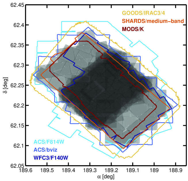
Figure 1.— Sky coverage of the multi-wavelength data sets used in the GOODS-N F160W catalog. The gray scale image shows the exposure time of the F160W mosaic, which includes the CANDELS wide and deep region. Coverage of ancillary data from UV to MIR are also shown: GOODS HST/ACS (blue), MOIRCS/MODS Ks (red), GTC/SHARDS optical medium-bands (orange), and GOODS Spitzer/IRAC (yellow). The entire field is covered by both SEDS Spitzer/IRAC and CFHT/K.

The CANDELS multi-wavelength photometric catalogs for the GOODS-S, UDS, COSMOS and EGS fields have been presented in Guo et al. (2013), Galametz et al. (2013), Nayyeri et al. (2017) and Stefanon et al. (2017), respectively; photometric redshifts and stellar population parameters for the first two fields are presented separately in Dahlen et al. (2013) and Santini et al. (2015). This paper presents the multi-wavelength catalog in GOODS-N, based on a CANDELS WFC3/F160W detection and making use of all the available ancillary data spanning from the UV to FIR wavelengths. Most notably, this catalog includes photometry in 25 medium-bands from the SHARDS survey (Pérez-González et al. 2013), which follows a similar observational strategy as previous optical surveys, such as COMBO17 (Wolf et al. 2001, 2003) and the COSMOS medium-band survey (Ilbert et al. 2009), but provides higher spectral resolution ($R\sim 50$) and deeper photometry (4$\sigma$, H$\sim 27$ mag) with an average sub arcsec seeing.

Furthermore, we expand the high spectral resolution coverage to the NIR by combining new WFC3 G102 grism observations with the publicly released G141 data from the 3D-HST survey (Momcheva et al. 2016), which yields a nearly continuous coverage from $\lambda=0.8-1.7$ $\mu$m with a resolution better than $R=130$. Lastly, we complement the optical and NIR photometry with a compilation of all the available FIR data from Spitzer and Herschel, spanning from $\lambda=24-500$ $\mu$m.

This paper is organized as follows: § 2 briefly summarizes the photometry datasets included in our catalog. § 3 discusses the detection process in the CANDELS F160W image and photometry measurements on the HST and mid-to-low spatial resolution images. § 4 presents several tests to evaluate the quality of the multi-band photometry. § 5 presents the added-value properties estimated from the fitting of the UV-to-FIR SEDs to stellar population and dust emission templates. The summary is given in § 6. The appendices describe the contents of photometric and added value the catalogs, released together with this paper, as well as the methodology to estimate self-consistent SFRs.

The CANDELS GOODS-N multi-wavelength catalog and its associated files are made publicly available on the Mikulski Archive for Space Telescopes (MAST). They are also available in the Rainbow Database(Pérez-González et al. 2008; Barro et al. 2011), either through Slicer, which allows a direct download of images and catalogs, or through Navigator, which features a query menu that allows users to search for individual galaxies, create subsets of the complete sample based on different criteria, and inspect cutouts of the galaxies in any of the available bands.

All magnitudes in the paper are on the AB scale (Oke 1974) unless otherwise noted. We adopt a flat ${\rm\Lambda CDM}$ cosmology with $\Omega_{m}=0.3$, $\Omega_{\Lambda}=0.7$ and use the Hubble constant in terms of $h\equiv H_{0}/100{\rm km~{}s^{-1}~{}Mpc^{-1}}=0.70$.

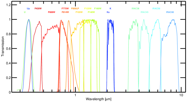
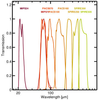
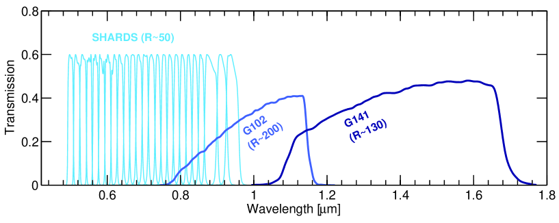
Figure 2.— Top: Transmission curves of all the broad-band filters used in the CANDELS GOODS-N multi-wavelength catalog, from the UV, optical and NIR (left) to the FIR (right). Bottom: Transmission curves of the higher spectral resolution data: the optical medium-band survey SHARDS ($R\sim$50), and the two HST/WFC3 grisms, G102 ($R\sim 200$) and G141 ($R\sim 130$). The panel above shows the redshifts ranges in which the most prominent emission lines (H$\alpha$, [Oiii], H$\beta$ and [Oii]) can be detected in each of these higher resolution dataset.

2. Imaging Datasets

The GOODS-N field (Giavalisco et al. 2004), centered around the Hubble Deep Field North (HDFN Williams et al. 1996) at $\alpha$(J2000) = 12^h36^m55^s and $\delta$(J2000) =+62^∘14^m11^s, is a sky region of about 171 arcmin² which has been targeted for some of the deepest observations ever taken by NASA’s Great Observatories: HST, Spitzer, and Chandra as well as by other world-class telescopes (see Figure 1).

The multi-wavelength coverage of GOODS-N spans from X-ray, UV to far IR and radio data: UV data from GALEX (PI C. Martin), ground-based optical data from $U$ to $z$ bands taken by the Kitt Peak 4-m telescope and from Suprime-Cam on the Subaru 8.2-m as a part of the Hawaii Hubble Deep Field North project (Capak et al. 2004), 25 medium-bands from the GTC SHARDS (Pérez-González et al. 2013) survey, near infrared (NIR) J, H and Ks imaging from the Subaru MOIRCS deep survey (Kajisawa et al. 2009) and CFHT/WIRCam Ks photometry (Hsu et al. 2019); IRAC maps from Spitzer GOODS (Dickinson et al. 2003), SEDS (Ashby et al. 2013) and SCANDELS (Ashby et al. 2015); MIPS data from GOODS-FIDEL (PI: M. Dickinson); Herschel from the GOODS-Herschel (Elbaz et al. 2011) and PEP (Magnelli et al. 2013) surveys.

In the following we provide more details about the datasets included in the multi-band catalog. The telescope/instrument as well as the reference for the survey are given in Table 1. Table 2 lists the central wavelength of the filters, dust attenuation from Galactic extinction, image zero point and the average FWHM for each of the mosaics. Transmission curves for all filters are plotted in Figure 2 .

2.1. HST

2.1.1 ACS Optical imaging

The HST/ACS F435W, F606W, F775W, and F850LP images used in our catalog are the version v3.0 of the mosaicked images from the GOODS HST/ACS Treasury Program. They consist of data acquired prior to the HST Servicing Mission 4, including mainly data of the original GOODS HST/ACS program in HST Cycle 11 (GO 9425 and 9583; see Giavalisco et al. 2004) and additional data acquired in HST/ACS F606W and F814W as part of the CANDELS survey and during the search for high redshift Type Ia supernovae carried out during Cycles 12 and 13 (Program ID 9727, P.I. Saul Perlmutter, and 9728, 10339, 10340, P.I. Adam Riess; see, e.g., Riess et al. 2007).

2.1.2 WFC3 IR imaging

The CANDELS survey observed the GOODS-N field in 3 HST/WFC3 IR filters F105W, F125W, and F160W following a “wedding-cake” observing strategy similar to that in the CANDELS/GOODS-S field but with only 2 layers, deep and wide (i.e., there is no ultra-deep region). The deep region consists of a rectangular grid of 3$\times$5 pointings that covers the central one-third of the mosaic (see Figure 1) with an approximated area of $\sim$55 arcmin² ($\sim 35\%$ of the mosaic). The observations were done over 10 epochs at 6 to 8 orbit depth in F125W and F160W. The wide region covers the northern and southern two-thirds of the field ($\sim 50\%$ of the mosaic) with 2$\times$4 pointings in both filters and has approximately 2-orbit exposures. The distributions of exposure time and limiting magnitude of the F160W mosaic are shown in Figure 3. An intermediate-depth region (between $\sim$4 and 9ks) is defined by the overlapping area between the wide and deep regions. The CANDELS F105W observations consist only of the deep and wide regions with a exposure gap in the intermediate region. See Grogin et al. (2011) and Koekemoer et al. (2011) for more details of CANDELS HST/WFC3 observations and data reduction. We also include in our catalog the 2-orbit depth F140W images taken as a part of the G141 AGHAST survey GO: 11600 (PI: B. Weiner; see next section) and GO:12461 COLFAX (PI: Riess).

The WFC3 mosaics used in this paper have been reduced following the same data reduction strategy described in the previous CANDELS data release papers for the other fields. The images in all bands are drizzled to 0$\farcs$06/pixel to match the default CANDELS pixel scale (see Koekemoer et al. 2011, for details).

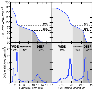
Figure 3.— Distributions of exposure time and limiting magnitude of the F160W mosaic used as the detection image of our catalog. The left column shows the cumulative (upper panel) and differential (lower) distributions of the exposure time, while the right column shows the same distributions of 5$\sigma$ limiting magnitude of the image.

2.1.3 WFC3 G102 and G141 grism spectroscopy

The GOODS-N field was observed in the HST/G141 grism at a 2-orbit depth as a part of the AGHAST program (GO:11600; PI: Weiner). The 28 pointings of the program were reduced, analyzed and incorporated to the 3D-HST survey (Brammer et al. 2012; Momcheva et al. 2016), which uses a similar observing strategy over the other 4 CANDELS fields. Each pointing was observed for two orbits, with $\sim$800 s of direct imaging in the F140W filter and 4511-5111 s with the G141 grism per orbit. The observations were arranged in a 4$\times$6 grid. There is no imaging or grism spectra in the northwestern edge of the field (dark blue line in Figure 1). In this paper we make use of the 3D-HST spectra released in their v4.1.5 data products described in Momcheva et al. (2016).

Furthermore we present complementary HST/G102 observations (GO:13179; PI: Barro) that were designed to follow the same tiling strategy of AGHAST program in other to maximize the number of galaxies with simultaneous grism coverage. The observations consist of 28 two orbit depth pointings with 400 s of direct imaging in the F105W filter and $\sim$5000 s with the G102 grism per orbit following the same 4-point dither pattern of 3D-HST survey. The observations were processed using the 3D-HST data reduction pipeline described in Momcheva et al. (2016). The pipeline combines the individual G102 exposures into mosaics using AstroDrizzle (Gonzaga & et al. 2012). These individual exposures are aligned using tweakreg and grism sky backgrounds are subtracted using master sky images as described by (Brammer et al. 2015). Each exposure is then interlaced to a final image with a pixel size of $\sim 0\farcs 06$. Before sky-subtraction and interlacing each individual exposure was checked and corrected for elevated backgrounds due to the He Earth-glow using the script described by (Brammer et al. 2014).

From the final G102 mosaics, the spectra of each individual object are extracted by predicting the position and extent of each two-dimensional spectrum based on the SExtractor (Bertin & Arnouts 1996) segmentation of the CANDELS F160W image. As this is done for every single object, the contamination, i.e., the dispersed light from neighboring objects in the direct image field-of-view is estimated and accounted for. We also carried out visual inspections of the individual 2D and 1D extractions for a magnitude limited subset of the data (F105W$<23$ mag) in order to flag catastrophic failures. The automated redshift determination and the emission line measurements based on these G102 and G141 datasets are presented in § 5.2.

Table 1Image sources

Filters	Telescope/Instrument	Survey	Reference
$U$	KPNO 4m/Mosaic	Hawaii HDFN	Capak et al. (2004)
$U^{\prime}$	LBT/ LBC	-	Grazian et al. (2017)
25 medium-band optical	GTC / OSIRIS	SHARDS	Pérez-González et al. (2013)
F435W, F606W, F775W, F850LP	HST/ACS	GOODS	Giavalisco et al. (2004)
F814W	HST/ACS	CANDELS	Grogin et al. (2011); Koekemoer et al. (2011)
F105W, F125W, F160W	HST/WFC3	CANDELS	Grogin et al. (2011); Koekemoer et al. (2011)
F140W	HST/WFC3	AGHAST	GO: 11600 (PI: B. Weiner)
$K_{s}$	Subaru/MOIRCS	MODS	Kajisawa et al. (2011)
$K$	CFHT/Megacam	-	Hsu et al. (2019)
3.6, 4.5 $\mu$m	Spitzer/IRAC	SEDS	Ashby et al. (2013)
5.8, 8 $\mu$m	Spitzer/IRAC	GOODS	Dickinson et al. (2003)
24, 70 $\mu$m	Spitzer/MIPS	GOODS/FIDEL	Dickinson et al. (2003)
100, 160 $\mu$m	Herschel/PACS	PEP	Berta et al. (2011), Lutz et al. (2011)
250, 350, 500 $\mu$m	Herschel/SPIRE	GOODS/Herschel, HerMES	Oliver et al. (2012),Magnelli et al. (2013)

2.2. Ground-Based Imaging

2.2.1 Ultraviolet

The $U$-band image was taken with the Mosaic camera on the Kitt Peak 4-m telescope by the Hawaii Hubble Deep Field North project (Capak et al. 2004).

In addition to the Kitt Peak imaging, an LBT Strategic Program (PI A. Grazian) was approved on 2012B, with the aim of obtaining ultra deep imaging in the U band of the CANDELS/GOODS-N field using the LBC instrument at the prime focus of the LBT telescope (Giallongo et al. 2008; Rothberg et al. 2016). The program consisted on approximately 25 hours on a single pointing of the LBC camera. The LBC field of view is larger than the whole CANDELS/GOODS-N field, and it covers approximately 600 sq. arcmin. with homogeneous coverage/depth. The same area has been observed also by other LBT partners (AZ, OSURC, and LBTO), for a total exposure time of 33 hours in U band (seeing 1.1 arcsec). The detailed description of these data is provided in a dedicated paper (Grazian et al. 2017) summarizing all the LBC deep observations available in the CANDELS fields. The relatively long exposure time and the good seeing allowed to reach a magnitude limit in the U band of 30.2 AB at S/N=1, resulting in one of the deepest UV images ever obtained.

2.2.2 SHARDS Optical medium-band survey

The Survey for High-z Absorption Red and Dead Sources (Pérez-González et al. 2013, SHARDS), an ESO/GTC Large Program, targeted the GOODS-N field with GTC/OSIRIS in 2012-2015 and obtained 220 hours of ultra-deep imaging data through 25 medium-band optical filters. The wavelengths covered a range from 500 to 950 nm with a spectral resolution of $R\sim 50$. The depth is 26.5 mag at the $4\sigma$ level (at least) and the seeing was always below 1″ for every single filter. SHARDS used 2 OSIRIS (FOV 7.8′$\times$7.8′) pointings to cover most of the CANDELS region (110 $\rm{arcmin}^{2}$). The SHARDS optical imaging data has a particular characteristic that has to be taken into account to obtain accurate spectral energy distributions: the passband of the filter seen by different parts of the detector changes, getting bluer as we move away from the optical axis, which is located about 1′  to the left of the FOV. Therefore, every galaxy detected by SHARDS counts with a unique set of SHARDS passbands, which are defined by their transmission curves (whose shapes does not change and, therefore, are the same for all galaxies) and their central wavelengths (which change and must be provided for each galaxy). We remark that this is an optical effect which affects all filters, so the final spectral energy distribution for each galaxy counts with the same spectral resolution, $R\sim 50$, but all the filters are offsetted from the nominal central wavelength. In order to properly account for this effect, the SHARDS photometry of the F160W sources (see § 3.2) is provided in a separated catalog (see Table A2) which includes the central wavelength for each galaxy and filter. Furthermore, the SHARDS science images in each of the 25 filters, which are released with this paper, are provided jointly with a map of the central wavelength for each pixel that can be used to account for the wavelength shift (see Pérez-González et al. 2013 for more details).

2.2.3 Near Infrarred

Deep $K_{s}$-band images of the field were taken using Multi-Object Infrared Camera and Spectrograph (MOIRCS) on Subaru as part of the MOIRCS Deep Survey (MODS, Kajisawa et al. 2011).. The data reach 5$\sigma$ total limiting magnitude for point sources of $K_{s}=24.2$ over a 103 arcmin² mosaic consisting of 4 MOIRCS pointings. The central $\sim$28 arcmin² of the mosaic contains a deeper region were the data reach $K_{s}=25.1$. In this work we make use of the publicly available “convolved” mosaic in which each of the four pointings have been homogenized to match the field with the worst seeing (FWHM$\sim$0$\farcs$6).

In addition to the MOIRCS data, we also make use of a deep broad-band $K_{s}$ mosaic based on observations with the CFHT WIRCam instrument (Hsu et al. 2019). The final mosaic used in this paper covers $\sim$0.4 square degrees around the GOODS-N field. It has a 50% completeness limit for point sources between $K_{s}=24.6-24.8$ mag. The astrometry was calibrated using the Two Micron All Sky Survey (2MASS) catalog (Skrutskie et al. 2006) with a final internal accuracy of $\sim$0$\farcs$1.

2.3. Spitzer/Herschel mid-to-far IR

2.3.1 IRAC S-CANDELS

GOODS-N was observed by Spitzer/IRAC (Fazio et al. 2004) during the cryogenic mission in four bands (3.6, 4.5, 5.8, and 8.0 $\mu$m) for two epochs with a separation of six months (February 2004 and August 2004) by the GOODS Spitzer Legacy project (PI: M. Dickinson). Each epoch contained two pointings, each with total extent approximately 10 arcmin on a side. The exposure time per band per sky pointing was approximately 25 hours per epoch and doubled in the overlap region. We use the 5.8 and 8.0 $\mu$m imaging from this program in our catalog.

The 3.6 and 4.5 $\mu$m photometry was measured on the mosaics from the Spitzer -CANDELS (S-CANDELS, PID 80216; Ashby et al. 2015) survey, which combines the original cryogenic data with that taken from the warm mission phase. The resultant 3.6 $\mu$m and 4.5 $\mu$m mosaics fully cover the WFC3 F160W area of the CANDELS survey to a depth of at least 50 hours. The IRAC data in all 4 bands were reprocessed and mosaicked using the same CANDELS HST tangent-plane projection and with a pixel scale of 0$\farcs$06/pixels, to prepare them appropriately for further photometric analysis (see also Ashby et al. 2015).

2.3.2 MIPS GTO, PEP & GOODS-Herschel

The GOODS-N field has been observed in the mid-IR wavelengths with Spitzer/MIPS at 24 $\mu$m and 70 $\mu$m as part of the GTO and GOODS surveys (Dickinson et al. 2003, see also Frayer et al. 2006). Here we use the photometric catalogs in both bands described in Pérez-González et al. (2005, 2008) which are based on the reduced and mosaicked data. Furthermore, far-IR observations with the Photodetector Array Camera and Spectrometer (PACS; Poglitsch et al. 2010) and the Spectral and Photometric Imaging REceiver (SPIRE; Griffin et al. 2010), on board the Herschel Space Observatory were obtained as part of the PACS Evolutionary Probe (PEP; Berta et al. 2011; Lutz et al. 2011), GOODS-Herschel (Magnelli et al. 2013) and HerMES (Oliver et al. 2012) surveys. The 5$\sigma$ detection limits of the far-IR data are provided in Table D1. The mid-to-far IR photometry probes the rest-frame wavelengths close to the peak of the dust IR emission of galaxies up redshifts of $z\sim 3$. Therefore it provides a very useful SFR indicator, complementary to the UV luminosity, for large number of galaxies. See § 3.3 and appendix D for a more detailed description of the IR data and the photometric measurements.

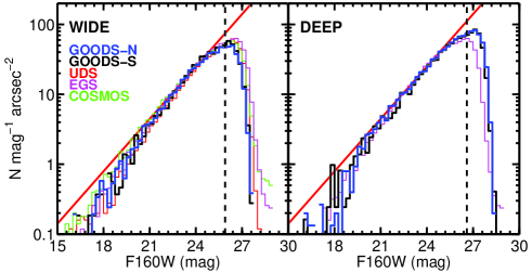
Figure 4.— Differential number counts for objects detected in the GOODS-N F160W catalog on the wide (left) and deep (right) regions. The different histograms show the number counts in all 5 CANDELS fields for comparison. The UDS, COSMOS and EGS fields were only observed to “wide” depth. The solid red line in each panel shows the best power-law fit to the number counts in the magnitude range where the sample is complete.

2.4. Value-added data

2.4.1 Spectroscopic Redshifts

A number of different spectroscopic observations were conducted in the GOODS-N field over the course of the last 20 years. Here we include redshift compilations based primarily on large spectroscopic surveys using the Keck/DEIMOS optical spectrograph: the ACS-GOODS redshift survey (Cowie et al. 2004; Barger et al. 2008), the Team Keck Redshift Survey Wirth et al. 2004, TKRS) and the DEEP3 galaxy redshift survey (Cooper et al. 2011). We also included redshifts from a number of other smaller surveys that often targeted specific types of objects or small regions defined by observations with new instruments: Lyman-Break galaxies (Reddy et al. 2006), bright-IR galaxies (Pope et al. 2008), sub-mm galaxies (Chapman et al. 2005) or the ACS-grism PEARS survey (Ferreras et al. 2009). Furthermore, we complemented these optical redshifts with results from recent NIR spectroscopic campaings using the Keck/MOSFIRE spectrograph that are critical to increase the number of secure spectroscopic redshifts beyond $z\sim 1.5$ : the 1st epoch of the MOSFIRE Deep Evolution Field (MOSDEF) survey (Kriek et al. 2015) and the TKRS2 (Wirth et al. 2015). The extensive spectroscopic campaigns in GOODS-N yield a total of $\sim$5000 unique redshifts within the CANDELS F160W mosaic coverage, and $\sim$3000 of those with a highly reliable quality flag. The counterparts to the spectroscopic sources were identified using a crossmatch radius of 0$\farcs$8 (if more than one object falls within the matching radius, the closest match with the highest confidence flag was adopted). All spectroscopic identifications are listed in the catalogs, but only those with reliable quality flags are used in the analysis of galaxy properties.

2.4.2 X-ray

We used X-ray data from the Chandra 2 Ms source catalog by Alexander et al. (2003), covering the entire surveyed region of the F160W mosaic in GOODS-N, to select candidates to harbor an AGN within our sample. The most likely X-ray counterparts to the CANDELS sources were identified using a cross-matching radius of 2$\farcs$5 between the CANDELS F160W catalog and the X-ray catalog of Alexander et al. (2003). We identify a total of 316 X-ray sources with a reliable F160W counterpart. This makes $\sim 3\%$ of all the sources in the F160W catalog down to $H<24.5$.

Table 2GOODS-N Optical-to-NIR Imaging

Band	$\lambda_{\mathrm{central}}$	$A_{\lambda}$	Zero Point	FWHM	ZP-corr	$5\sigma$ Depth
	($\mu m$)	(mag)	(AB)	(arcsec)	(flux)	(mag)
U	0.35929	0.052	31.369	1.26	0.88	26.7
U’	0.36332	0.052	26.321	1.10	1.07	28.2
F435W	0.43179	0.044	25.689	0.10	1.03	27.1
SHARDS	0.50-0.94	-	-	-	-	-
F606W	0.59194	0.030	26.511	0.10	0.97	27.7
F775W	0.76933	0.020	25.671	0.11	0.98	27.2
F814W	0.76933	0.020	25.671	0.11	0.97	28.1
F850LP	0.90364	0.015	24.871	0.11	1.02	26.9
F105W	1.24710	0.009	26.230	0.18	1.03	26.4
F125W	1.24710	0.009	26.230	0.18	1.01	27.5
F140W	1.39240	0.007	26.452	0.18	1.04	26.9
F160W	1.53960	0.006	25.946	0.19	1.03	27.3
K	2.13470	0.004	26.000	0.60	0.92	24.4
Ks	2.15770	0.004	26.000	0.60	0.96	24.7
IRAC1	3.55690	0.000	21.581	1.7	0.93	24.5
IRAC2	4.50200	0.000	21.581	1.7	0.90	24.6
IRAC3	5.74500	0.000	20.603	1.9	0.87	22.8
IRAC4	7.91580	0.000	21.781	2.0	0.80	22.7

3. Photometry

This section discusses the methods used to assemble the UV-to-FIR multi-wavelength photometric catalog. The following subsections describe the procedures to identify and characterize all the sources detected in the WFC3/F160W image and to obtain self-consistent photometric measurements in the high, intermediate, and low resolution photometric datasets.

3.1. High resolution HST data

3.1.1 WFC3 F160W detection and photometry

We follow a similar approach as in the previous four CANDELS data papers (Guo et al. 2013; Galametz et al. 2013; Stefanon et al. 2017; Nayyeri et al. 2017). We identify sources using the reddest NIR band, WFC3/F160W, mosaic. Both source detection and photometry were performed using a slightly modified version of SExtractor v2.8.6 (Bertin & Arnouts 1996) that fixes some known issues that often cause the inclusion of false detections in the final catalog merged with real sources, and a sky over-subtraction that could affect faint extended sources (see Galametz et al. 2013).

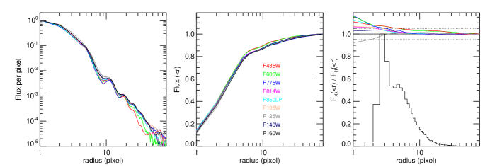
Figure 5.— Accuracy of PSF matching between other HST bands and F160W. Left: the light profile of matched PSFs for each band. Middle: the curve of growth of each matched PSF. Right: the curve of growth of each matched PSF normalized by the curve of growth of the F160W PSF. In this panel, curves with values greater than unity are under-smoothed, and vice versa. All curves are color coded as labels in the middle panel show. Dotted lines in the right panel show the 5% relative error. The solid histogram in the right panel shows the distribution of isophotal radii of all objects in our catalog.

The source detection is based on the 2-step “cold” plus “hot” strategy described in more detail in the CANDELS UDS (Galametz et al. 2013) and GOODS-S (Guo et al. 2013) papers. Briefly, we ran SExtractor twice using two different parameter configurations (see Table 3) aimed at: detecting bright/large sources without over-deblending them (cold-mode), or pushing the detection limit to recover faint sources close to the limiting depth of the mosaic (hot-mode). Then, we merge the cold and hot catalogs following a similar approach as the GALAPAGOS code (see Barden et al. 2012 for more details). All cold-mode detected sources are included in the merged catalog, but only those hot-mode sources whose segmentation map does not overlap with the photometric (Kron 1980) ellipse of a cold-mode source are included, i.e., hot-mode sources that are clearly overlapping with a cold-mode detection or the result of excessive shredding are excluded from the merged catalog. We detect 35445 sources in the F160W mosaic. Among them, 27293 sources are detected by the cold mode and 8152 sources by the hot mode.

Figure 4 shows the distribution of detected sources in the F160W mosaic as a function of magnitude (i.e., the differential number counts). The left panel depicts the number counts in the GOODS-N wide region compared to those measured in regions of similar depth in the other 4 CANDELS fields. All the measurements are in good agreement up to $H\sim$ 24 mag. As pointed out in Stefanon et al. (2017), the number counts in the wide region of the GOODSs and COSMOS fields are slightly below those in the UDS and EGS measurements in the $24<H<26.5$ range, most likely due to the slightly deeper data (0.2 mag) in EGS compared to those fields. The right panel of Figure 4 compares the number counts in the deep regions of GOODS-N and GOODS-S, which are consistent up to $H\sim 29$ mag.

As expected, the bulk of the number counts are consistent with those in the wide region (the counts in EGS are shown again as reference), while the number of detections at fainter magnitudes $H\gtrsim 26$ increases. The differential variation of the number counts in the faint end can be used to assess the completeness of the catalog. Following the approach in Guo et al. (2013), we fit the number counts in the region were the catalog is expected to be complete ($20<H<24$) with a power-law of slope $\gamma=0.20\pm 0.06$. Then, we find the $\sim 50\%$ completeness limit by computing the magnitude where the relative difference between the observed counts and the power-law reaches a factor of two: $H\sim 25.9$ and 26.6 mag in the wide and deep regions, respectively (dashed lines in Figure 4). These values agree with the completeness limits of the CANDELS/GOODS-S catalog at similar depths (see also Fig. 3 of Duncan et al. 2014). We refer the reader to Guo et al. (2013) for a more detailed discussion on the dependence of the completeness limit with the surface brightness profiles of the galaxies in GOODS-S. Given the similar depths of the GOODSs fields, those results are directly applicable to the GOODS-N catalog.

Table 3SExtractor Parameters in Cold and Hot Modes

	Cold Mode	Hot Mode
DETECT_MINAREA	5.0	10.0
DETECT_THRESH	0.75	0.7
ANALYSIS_THRESH	5.0	0.8
FILTER_NAME	tophat_9.0	gauss_4.0
DEBLEND_NTHRESH	16	64
DEBLEND_MINCONT	0.0001	0.001
BACK_SIZE	256	128
BACK_FILTERSIZE	9	5
BACKPHOTO_THICK	100	48
MEMORY_OBJSTACK	4000	4000
MEMORY_PIXSTACK	400000	400000
MEMORY_BUFSIZE	5000	5000

3.1.2 Photometry Flags

At this stage we also assigned a photometry flag to every object in the catalog. The flagging system is the same adopted in previous CANDELS papers and discussed in detail by Galametz et al. (2013). Briefly, the flagging scheme is based on the properties of the F160W mosaic. We use a zero for sources with reliable photometry and assigned a value of one either for bright stars or spikes associated with those stars. The radius of the star’s masks range between $3-5\arcsec$ for $\sim$20 intermediate brightness stars and 10$\arcsec$ for the 2 brightest stars in the field. A photometric flag of two is associated with the lower exposure edges of the mosaic or defects as measured from the F160W RMS maps. This is a very conservative flag assigned only to pixels with extreme ($>$1E5) values of the RMS map.

3.1.3 Optical/NIR HST photometry

The photometry in all other HST bands $-$ ACS F435W, F606W, F775W, F814W, F850LP and WFC3 F105W, and F125W was measured running SExtractor in dual mode using the F160W mosaic as reference to ensure that the colors are measured within apertures of the same size. This means that the multi-band photometry is computed only for the sources detected in the F160W mosaic. We follow the same cold+hot routine described in the previous section by running SExtractor twice per band. In order to take into account the variations in spatial resolution as a function of wavelength (see the typical FWHMs of the HST bands in Table 2) all HST images were previously smoothed to the lower spatial resolution of F160W (FWHM$\sim 0\farcs 18$) using the IRAF/PSFMATCH package with kernels that matched the multi-band PSFs with that of F160W. We computed semi-empirical PSFs in the WFC3 bands by combining a stack of isolated, unsaturated stars from across the mosaic with synthetic PSFs generated with TinyTim (Krist 1995). We used the central pixels from the synthetic models and the wings of stacked stars (see van der Wel et al. 2012 for more details). The ACS PSFs were based on purely empirical models computed by stacking well-detected stars, without any artifacts, in each ACS band.

The left panel of Figure 5 compares the stacked light profile of several high S/N stars, extracted from the deep region, in all HST bands after running PSFMATCH. The central and right panels shows also the curves of growth (fraction of light enclosed as a function of aperture size) in each band and the fraction of enclosed light relative to that of the F160W PSF. All profiles converge quickly to unity after a few pixels, and the relative photometric error in all HST bands is less than $5\%$ for apertures larger than two pixels (0$\farcs$12), which is larger than the typical isophotal radius for the bulk of the sources ($\gtrsim 97\%$).

We computed several different photometric measurements available in the SExtractor configuration, namely, FLUX_AUTO, measured on Kron elliptical apertures, FLUX_ISO measured on elliptical isophotes, and FLUX_APER measured in a series of 11 circular apertures (see appendix A for a description of all the measurements included in the photometric catalog). As discussed in the previous CANDELS data papers, we adopt FLUX_AUTO as the default “total” photometry for all the sources in the F160W band, while for the other bands we determine the total flux scaling FLUX_ISO by the ratio of FLUX_AUTO / FLUX_ISO in each band. This ratio is used to convert their isophotal fluxes and uncertainties into the total fluxes and uncertainties. The isophotal correction ensures that the flux is measured within the same isophotal area in all bands (defined by the F160W segmentation map) and maximizes the S/N for faint sources. This method provides an accurate estimate of colors and fluxes subject to the prior assumption that the PSF-convolved profile is the same in all bands. We verify the quality of the multi-band SEDs in § 4 by performing both internal and external checks, comparing to another catalog.

3.2. Intermediate resolution ground- and space-based data: TFIT

We computed multi-wavelength photometry in all the ancillary ground based data and in the Spitzer/IRAC bands using the TFIT code (Laidler et al. 2007) and following the same methodology described in the previous CANDELS data papers. TFIT is a template-fitting software conceived to overcome the issues related with obtaining consistent photometry across large datasets that exhibit significant differences in spatial resolution. The code uses accurate positional information of the sources in the highest resolution band (in this case HST/F160W) to create PSF-matched models (“templates”) of the sources in the intermediate resolution bands (e.g., ground-based K-band or IRAC). These “templates” are computed on an object-by-object basis by smoothing the high resolution cutouts to low-resolution using a convolution kernel (see e.g., Galametz et al. 2013). Then, the code fits iteratively for the photometry by comparing the real to the modeled images in those bands. With the simultaneous fitting approach, the code can take into account the flux contamination for each source due to their neighboring objects. The details of the software are described in detail in Laidler et al. (2007), Papovich et al. (2001) and (Lee et al. 2012) which includes a set of simulations to validate the photometric measurements and quantify its uncertainties. See also Merlin et al. (2015, 2016) for further tests and improvements on the code, branched as T-PHOT. For this paper we chose to use the original TFIT for consistency with all the previous CANDELS catalogs and also with early internal releases of the GOODS-N catalog.

In the following, we briefly summarize the main steps involved in the TFIT photometric measurements. Before running the fitting code, we perform an additional background subtraction step of the intermediate resolution images to ensure that there are no inhomogeneous regions that could potentially bias the photometry. The iterative background fitting script is based on an IRAF script “acall” originally developed for GOODS (M. Dickinson 2013, private communication; see Guo et al. 2013 for more details). Then, the images are re-sampled to a pixel scale that is a multiple of the F160W pixel scale (e.g., $\sim 10\times$ for Spitzer/IRAC) using SWARP (Bertin 2010). Lastly, we identify and stack several bright, isolated stars in each band to determine its average PSF and to compute the transformation kernel required to match the PSF of the high resolution F160W band. The fitting “templates” for each galaxy are computed by convolving their F160W segmentation maps with such kernels. As discussed in the previous CANDELS data papers, we apply a small “dilation” correction to the F160W segmentation map to avoid an artificial truncation of the light profiles of the sources. The dilation factor was determined following the empirical relation in Equation 3 of Galametz et al. (2013).

We run TFIT separately in all the ground based and Spitzer/IRAC images. As mentioned above, the flux for each object is determined by fitting its template, and those of the neighboring objects, to the intermediate resolution image, thus obtaining a direct estimate of the possible flux contamination due to blending. The code runs the fitting step twice, and the second iteration allows for small shifts in the PSF-matched kernels to improve lower quality fits caused by small image distortions in the intermediate resolution images. Figure 6 shows examples of the TFIT residual map i.e., the result of subtracting the best-fit object templates from the original image, in three bands with different spatial resolutions demonstrating that the fitting procedure was successful.

With the “dilation” correction, included to avoid flux loss in the outskirts regions of fainter objects, and assuming that the morphology of the segmentation map is not strongly dependent on the wavelength, we can consider the fluxes measured with TFIT analogous to the “total” fluxes measured with SExtractor’s FLUX_AUTO (see also Lee et al. 2012 and Merlin et al. 2015). Therefore, we apply no further corrections to these flux measurements. The merged photometric catalog combines the HST fluxes measured with SExtractor and the TFIT fluxes for the intermediate resolution bands. A quantitative analysis of the quality of the photometric catalog is presented in § 4

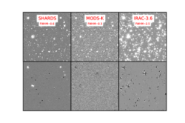
Figure 6.— Example of the original image (top) and the residual image after TFIT procedure (bottom) of several low-resolution bands as indicated in the upper panels in a representative sky region. Positive residuals in SHARDS and IRAC images are due to saturation around bright sources.

3.3. Low resolution mid-to-far IR data

Here we describe the procedure to assign mid-to-far IR photometry to the F160W sources. Given the significant differences in depth and resolution between the optical/NIR and the IR imaging this procedure consists of two steps. First, we build a self-consistent IR catalog using only Spitzer and Herschel data. This merged IR catalog combines prior-based extractions and direct detections starting from the higher resolution Spitzer IRAC and MIPS bands all the way up to the low resolution SPIRE bands. Second, we assign those IR-fluxes to some of the CANDELS/F160W sources by crossmatching the IR-only and F160W catalogs and identifying the most likely NIR counterparts to the IR detections based on brightness and proximity criteria. In the following we briefly describe the main steps of the method. A more detailed description is provided in appendix D.

We start by building merged, mid-to-far IR photometric catalogs using the imaging datasets introduced in § 2.3. The procedure to carry out the source detection and to measure the photometry is described in detail in appendix D, as well as several other previous works, Pérez-González et al. (2010, see also and ). Briefly, the method consists of three steps: (1) source identification in each of the IR bands starting from the deeper and higher resolution bands at shorter wavelenghts and progressing towards redder, lower resolution bands by using a combination of priors and direct detections, (2) photometric measurements based on PSF fitting and aperture photometry, and (3) merging of the individual photometric catalogs to produce merged, multi-band, MIPS, PACS, and SPIRE catalogs. Overall, the merged IR catalog contains of the order of a few thousand detections at 24 $\mu$m and a few hundred in the PACS and SPIRE bands. This implies that the multiplicity of F160W detections per IR source ranges between 5 to 10. Thus, in order to obtain a 1 to 1 match of the two catalogs, it is necessary to identify the most likely counterparts on the basis of their NIR brightness and their coordinates in the high resolution images.

To do so, we run a crossmatching procedure sequentially from high-to-low resolution bands, starting from F160W to MIPS, then MIPS to PACS and lastly PACS to SPIRE. This method minimizes the multiplicity of each crossmatch by chosing far IR pairs with relatively small differences in resolution ($\sim 1.5\times$). Then, we choose the most likely counterpart from those within the matching radius by prioritizing brightness and proximity to the low resolution source. The crossmatch with the largest multiplicity is F160W to MIPS, where the difference in resolution is almost $20\times$. However, in this case the brightness in the reddest IRAC band at 8 $\mu$m is a very effective discriminator, as it probes the rest-frame mid-IR region (at $z\lesssim 1.5$) which often exhibits a flux contribution from the dust emission in addition to the stellar continuum. Based on the sequential counterpart identification, each mid-to-far IR source has a unique F160W counterpart in the final catalog. Nonetheless, we provide supplementary IR catalogs (see appendix D.4) which indicate all the secondary short-wavelength counterparts in each of the IR bands involved in the crossmatching procedure. These catalogs also indicate the crowdness, i.e., the total number of counterparts to each long-wavelength, IR source, which can be used for further diagnostics.

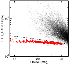
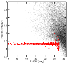
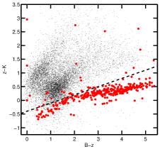
Figure 7.— Left: SExtractor’s FLUX_RADIUS against total F160W magnitude. Objects classified as point sources in the catalog are shown with red circles. The black dashed line indicates the selection criterion. Center: alternative selection method based on the ratio of fluxes measured in large (2$\farcs$0) and small apertures (0$\farcs$5). The stellar sequence (corresponding to the selection criterion of the left panel) at brighter magnitudes ($H<24$ mag) is tighter with this method. However, the separation from extended sources is less clear at fainter magnitudes. Right: $BzK$ color-color diagram showing another alternative method to identify stars (and galaxies; e.g. Daddi et al. 2005). The $BzK$ diagram shows an excellent agrement with the other two methods for bright stars (red). However, a color-based selection (dashed black line) would also include a significant fraction of faint and less realiable sources. Note also that the $BzK$ diagram relies on ground-based photometry which is shallower than the F160W mosaic.

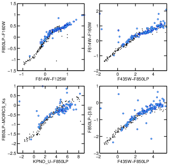
Figure 8.— Color-color diagrams comparing the CANDELS GOODS-N photometry of unresolved sources classified as stars in blue (see § 4.1), and model stars in black from the Gunn & Stryker (1983) Atlas of stars. The model colors of stars are computed in each filter by integrating the model SED of stars from the library over the filter transmission curves.

4. Quality Assessment

In this section we test the quality of the photometric catalog by (1) comparing the observed colors of stars to those estimated from stellar libraries, and (2) comparing the fluxes in our catalog to other published catalogs in GOODS-N. Furthermore, in Section 5 we also analyze several added value properties computed from the fitting of the UV-to-FIR SEDs, which depend on the quality of the photometric measurement described in the previous section.

4.1. Star identification and colors

We compare the observed colors of the stars in our catalog to those estimated from a stellar library. We use the synthetic models of stars from the Bruzual-Persson-Gunn-Stryker Atlas of stars (Gunn & Stryker 1983) that we convolve with the response curves of the different filters. Stars (unresolved sources) can be identified using a size-magnitude diagram, as they form a tight sequence with fairly constant small sizes as a function of magnitude. The left panel of Figure 7 shows the SExtractor FLUX_RADIUS against the total F160W magnitude for all the sources in the catalog. Point sources (red circles) can be cleanly separated from extended sources down to $H\sim 25$ mag using the following criterion: FLUX_RADIUS $<-0.115H+5.15$ (see also Skelton et al. 2014 for a similar approach). We further verify the accuracy of this selection by comparing it with two alternative methods: 1) the ratio of the fluxes measured in large ($2\arcsec$) and small ($0\farcs 5$) apertures (central panel of Figure 7), which shows a similarly tight sequence at bright magnitudes ($H\leq 24$), and 2), the $BzK$ color-color diagram (Daddi et al. 2004), which is often used to isolate distant galaxies at $z>1.4$ (right panel of Figure 7), but it is also very effective at isolating a clear stellar locus.

We note here that for some of the HST/ACS bands in our catalog, particularly in F606W and F775W, the new mosaics created for this paper include both pre-service mission data (from GOODS and other smaller surveys) and new CANDELS data, which are separated in time by more than 5 years. As a result, the photometry of stars, some of which can have significant proper motions, is affected by systematics effects such as: (a) they have moved enough that they are partially falling out of the aperture defined by the F160W-band isophotes, and/or (b) that they are getting partially rejected as cosmic rays due to the motion. These effects are likely present as well in previous version of the mosaics (e.g., v2), meaning that stellar photometry for those stars in either set of mosaics is suspect.

Taking this into account, we compare the colors of stars, identified with the method described above, to those of stellar models excluding colors based on either the F606W and F775W bands (see next section for a comparison of the fluxes of non-stellar sources in these bands to the 3D-HST catalog). Figure 8 shows four of these diagrams. The observed colors of the point-like objects (blue circles) are consistent with the general distribution predicted by the stellar models showing no systematic biases. This further confirms the accuracy of the photometry, specifically for the brighter sources.

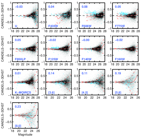
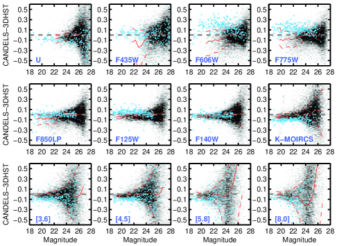
Figure 9.— Photometric comparison between the CANDELS and 3D-HST multi-wavelength photometry in the GOODS-N field. Top: – Magnitude difference (CANDELS-3DHST) vs. CANDELS magnitude in all the bands in common between the two catalogs. For each band, we only use sources with S/N$>$3 in both catalogs for comparison. The name of the bands is indicated in the bottom-left corner. The median of the magnitude difference computed in the bright magnitude range (m=20–24 mag) is shown in the top-left corner. The grey scale density map shows all sources and the cyan points show stars. Both sets are corrected for the median magnitude difference to center the distributions around zero. The red solid line shows the running median (after a 3$\sigma$-clipping) of the magnitude difference as a function of magnitude. The upper and lower red dashed lines show 1$\sigma$ confidence level. Bottom: – Color difference in Band - F160W (CANDELS-3DHST) vs. CANDELS magnitude (e.g., top left panel is (U-F160W)_CANDELS -(U-F160W)_3D-HST vs U_CANDELS). The markers, lines and labels indicate the same as in the upper panel.

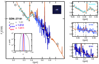
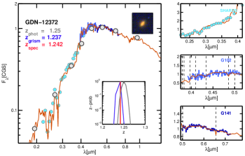
Figure 10.— SEDs of a star-forming (left) and a quiescent (right) galaxy in the CANDELS/GOODS-N region. The grey circles indicate broad-band photometry. The blue circles show the SHARDS medium-band data and the blue lines, from light to dark shading, the G102 and G141 grism spectroscopy. The rightmost panels in each figure show a zoom in into the key spectral regions for each of these datasets and highlight the most prominent emission and absorption features in the spectrum. The insets show the redshift probability distributions computed from the fitting to broad-band data (grey), and with the addition of SHARDS and grism data (blue). The red line indicates the spectroscopic redshift.

4.2. Comparison to other photometric catalogs

We compare our photometry with that of the 3D-HST multi-wavelength catalogs in GOODS-N (Skelton et al. 2014). The 3D-HST catalog includes 22 different photometric bands. The main difference between the latter and the CANDELS catalog in the optical-to-NIR bands is that CANDELS includes photometry in 25 optical medium bands from the SHARDS survey while the bulk of the optical ground-based data in the 3D-HST catalog is based on the broad-band photometry from the Hawaii Subaru survey (Capak et al. 2004). There is, however, direct overlap between the two catalogs in the HST optical and NIR bands as well as in the Spitzer/IRAC photometry and the $U$ and $K$ band data from Hawaii Subaru survey and the NIR MODS (Kajisawa et al. 2009), respectively.

The photometry of the 3D-HST catalog was performed following a similar methodology to ours (see Skelton et al. 2014 for a full description). Briefly, the photometry in the HST bands was computed using SExtractor in dual-image mode. The fluxes were measured in circular apertures and then corrected to total magnitudes based on a factor derived from curve of growth of the F160W PSF. The photometry in the lower-resolution bands was derived using a similar software to TFIT (MOPHONGO; Labbé et al. 2005, 2006, 2013). In addition to the aperture correction for the HST bands, two additional corrections were applied to account for Galactic extinction and small variations of the photometric zero-points. These two corrections are removed from the 3D-HST photometry before the comparisons described below.

We identify common sources between the CANDELS and 3D-HST catalogs by crossmatching the source coordinates with a maximum matching radius of 0$\farcs$3. We only include in the comparison cleanly detected sources (i.e., sources with good quality use-flag in both catalogs). The top panels of Figure 9 shows the magnitude difference between the CANDELS and 3D-HST photometric catalogs for all the bands in common between the two catalogs as a function of the magnitude in each band. For each band, we only consider objects with S/N$>$3 in both catalogs. Overall, the agreement is good, and the systematic offsets (corrected and indicated in the upper-left corner) over the high S/N magnitude range in most bands is of the order of a few hundredth of a magnitude. The small differences likely stem from the various systematic corrections that the 3D-HST catalog has applied. The largest offsets of the order of $\Delta$m$\sim$0.1-0.2 mag are found in the IRAC bands. These offsets are consistent with those found in the similar comparisons between the CANDELS and 3D-HST catalogs presented in previous CANDELS papers (Guo et al. 2013, Galametz et al. 2013, Nayyeri et al. 2017, Stefanon et al. 2017). Note that, as indicated in the previous section, the stellar loci for the HST/ACS bands F606W and F775W exhibits systematic deviations (cyan circles) because the positions of some stars in the merged multi-epoch mosaic have changed due to proper motions.

To further verify the accuracy of the photometry we also analyze the difference in the colors as a function of magnitude between the two catalogs, where the color is defined as the magnitude difference in a given band minus F160W. In principle, a color comparison is more straightforward as it should naturally factor out any dependence on the aperture correction. This comparison is shown in the bottom panels of Figure 9, and, again, we find an excellent agreement. Overall, these tests indicate that the flux measurements in both catalogs have been performed in a robust and self-consistent manner.

5. Added value properties

In this section we present the added value properties for the galaxies in the CANDELS GOODS-N catalog computed from the fitting of their UV-to-FIR SEDs to stellar population synthesis models and dust emission templates. We also present emission line measurements derived from the WFC3 G102 and G141 grism spectroscopy.

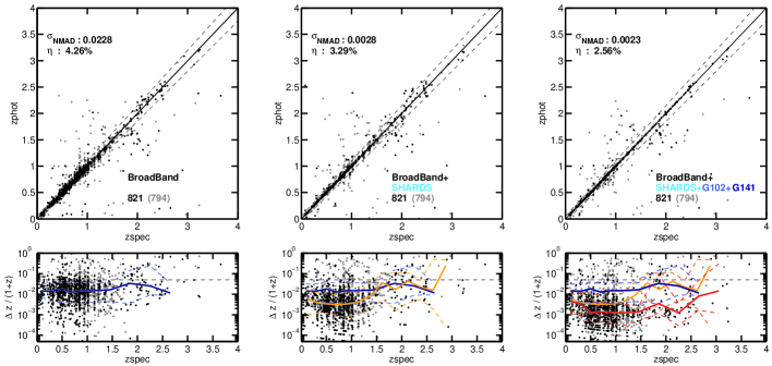
Figure 11.— Comparison of our multi-tiered photometric redshifts vs. spectroscopic redshifts for galaxies with both G102 and G141 spectra and good quality flag spectroscopic redshifts. The photometric redshifts are estimated using broad-band photometry only (tier 3, left), adding the SHARDS medium bands (tier 2, center), and adding the G102 and G141 grism spectroscopy to SED fit (tier 1, right). The black and grey circles indicate sources with high- and medium- quality spectroscopic redshift flag, respectively. The bottom panels shows the overall accuracy ($\Delta z/(1+z)$) of the photometric redshift as a function of redshift. The colored solid and dashed lines show the running median and 68% confidence regions. The black dashed line indicates the outlier threshold ($\Delta z/(1+z)=0.15$). Both the accuracy ($\sigma_{\mathrm{NMAD}}$) and the fraction of catastrophic outliers ($\eta$) improve with the addition of higher spectral resolution photometry.

5.1. Photometric redshifts

Here we discuss the photometric redshift estimates for the galaxies in the CANDELS GOODS-N catalog computed from SED fitting. The main difference between the galaxy SEDs in GOODS-N with respect to the other 4 CANDELS fields is that this catalog includes photometry in 25 medium-bands of the SHARDS survey ($R\sim 50$; $\lambda=0.50-0.95~{}\mu$m) and HST/WFC3 grism observations in both G102 and G141, thus allowing for a continuous wavelength coverage from $0.9\leq\lambda\leq 1.7\mu$m with a resolution of R$\sim 210$ and 130, respectively. Together, all these datasets provide remarkable spectral resolution on a galaxy-by-galaxy basis that is uniquely suited to provide high quality, SED-fitting based properties.

The use of higher spectral resolution photometric bands, such as medium or narrow band filters has been shown to improve the accuracy of the photometric redshifts up to the few percent level (e.g.; Ilbert et al. 2010; Whitaker et al. 2011; Straatman et al. 2016). The inclusion of WFC3 grism spectroscopy provides even higher spectral resolution capable of detecting emission lines, and thus provide redshift estimates of similar quality as those from typical, ground-based spectroscopic surveys (e.g.; Atek et al. 2010; Momcheva et al. (2016); Treu et al. 2015; Cava et al. 2015; Bezanson et al. 2016).

Given that the number of available spectro-photometric datasets for any given galaxy (i.e., whether they have SHARDS and/or grism data) depends on its magnitude and its location within the WFC3 mosaic we have implemented a three-tier classification for the photometric redshift estimates with increasing spectral resolution data. Tier 3 consists of photometric redshifts determined from broad-band photometry only. Although these redshifts are based on lower resolution data, they can be computed for all the galaxies in the catalog using the same set of input fluxes and therefore provide a uniform, homogeneous set of baseline redshifts. The second tier redshifts are based on the SED fitting to both broad-band and SHARDS medium band data, and the first tier includes broad and medium band data plus the WFC3 grism spectra. Roughly $\sim 80\%$ of the galaxies in the catalog lie in the region of GOODS-N covered by the SHARDS medium-band survey, and a large fraction of those, $\sim 60\%$ at $H<24$ mag, have also grism detections in either G141 or G102 (more details in § 5.1.5). All these galaxies have a more detailed SED coverage and, therefore, their photometric redshifts are likely to be more precise. In the following we describe the methods used to compute photometric redshifts for the galaxies in each of the three quality tiers.

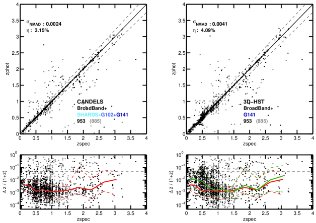
Figure 12.— Comparison of our photometric redshifts vs. spectroscopic redshifts (left) and the 3D-HST photometric redshifts (right) from Momcheva et al. (2016) which are based on broad-band photometry and G141 spectra. This comparison is restricted to galaxies with G141 spectra in both CANDELS and 3D-HST and having good quality spectroscopic redshifts. The lines in the bottom panels show the redshift evolution of the median $\Delta z/(1+z)$ for the CANDELS (red) and 3D-HST (green) samples. The addition of medium bands and the blue grism improves the quality of the photometric redshifts predominantly at low-z ($z\lesssim 0.7$), while both photometric redshift estimates are fully consistent at medium- and high-z. The colors of the points and lines have the same meaning as in Figure 11.

5.1.1 Tier 3: Broad-band based photometric redshifts

Following the same approach as in previous CANDELS papers we computed several estimates of the photometric redshifts using a number of different codes, e.g. EAZY (Brammer et al. 2008), HyperZ (Bolzonella et al. 2000), SpeedyMC (Acquaviva et al. 2011), etc, based either on $\chi^{2}$ and MCMC fitting methods and using different templates and SED modeling assumptions (see Appendix B for more details on all the different codes). As a common practice, each of the methods fine-tuned the performance of the photometric redshifts by computing small zeropoint corrections to the photometric fluxes by minimizing the difference between the observed fluxes and those expected from the best-fit templates. Since these corrections are dependent on the fitting codes and template libraries we followed the same approach as in the previous CANDELS data papers and we did not include such adjustments in the photometric catalog. However, we report the average photometric zeropoint offsets adopted by each group in Table 2.

As shown in Dahlen et al. (2013), using the median of multiple photo-z estimates provides a more accurate prediction of the true redshift and it helps mitigating some of the most common problems, such as systematic offsets and catastrophic outliers. Here we compute the median photometric redshift based on five different codes. All these codes used the same set of broad-band photometric data for all the galaxies in the sample. We adopt these median values as the tier 3 redshift estimates. Note that, while the tier 2 and 1 photometric redshift estimates presented in the following sections are significantly more accurate than the tier 3 redshifts for many galaxies, the tier 3 estimate is the only value available for those galaxies without SHARDS and/or grism coverage. Furthermore, since the improvement in the quality of the photo-z owing to the addition of high spectral resolution data is magnitude dependent, the tier 3 photo-z’s will also be very similar to tier 2 and 1 values for many faint, typically high-z, galaxies.

5.1.2 Tier 2: Broad and medium band photometry photometric redshifts

The tier 2 photometric redshift estimates are based on the fitting of the galaxy SEDs that include both broad band photometry and the 25 medium bands of the SHARDS survey. These redshifts are available to the nearly 80% of the galaxies which lie in the overlapping region between the CANDELS and SHARDS mosaics (see Figure 1). The photometric redshifts are computed using a slightly modified version of EAZY (Brammer et al. 2008) adapted to take into account the spatial variation in the effective wavelength of the SHARDS filters depending on the galaxy position in the SHARDS mosaics (see § 2.2.2).

5.1.3 Tier 1: Broad and medium band photometry plus grism spectroscopy photometric redshifts

The tier 1 photometric redshift estimates are based on the fitting of galaxy SEDs that include the broad and medium band photometry from tier 2 and the WFC3 grism spectroscopy. The accuracy of the grism-based photo-z’s depends critically on whether any prominent emission line falls within the observed spectral range (see e.g., Figure 2), and if such line is detected with high SNR. Given the limited spectral range of the grism, the majority of the emission line detections in either G141 or G102 consist of only one prominent line. However, if the SNR of that line is high enough (SNR$\gtrsim 5$), the use photo-z priors, such as the ones computed in tier 2 or 3, can help break the redshift degeneracies and provide a very precise redshift determination ($\Delta z\lesssim$1E-3; e.g. Momcheva et al. 2016).

In order to take full advantage of both the broad and medium band photometry and the grism spectroscopy, we computed the tier 1 photometric redshifts using the SED-fitting code developed by the 3D-HST survey and discussed in detail in Brammer et al. (2012) and Momcheva et al. (2016). This code was designed to estimate redshift probability distribution functions (PDFz) based on the constraints from the broad- and medium-band photometry as well as their G141 grism spectroscopy. Here we use a slightly modified version of the code which makes use of both the G102 and G141 spectroscopy in this calculation. Briefly, the redshift determination is done iteratively in three steps, first using only the photometric SED to obtain coarse constraint on the PDFz, then fitting the grism data alone over a finer redshift grid, and lastly fitting both together multiplying the likelihood of all the redshift distributions. The first iteration of the fitting uses the preliminary photo-z estimate from the previous section as a prior on the fit to broad and medium-band photometry. The fit to the grism spectrum is done in 2D to take into account the impact of the spatial extent of the source in the spectral direction. This is done by using the SExtractor segmentation map of each source in the direct F105W and F140W images for G102 and G141, respectively.

An advantage of the iterative fitting method is that the resulting PDFz defaults to the tier 3 or 2, photometry-only solution in all the cases where there is no significant contribution to the probability distribution from the fit to the grism data. Thus, the improvement in the accuracy of the PDFz over the photometry-only case depends on the significance of detected features on the grism spectra, e.g., strong emission lines, continuum breaks or absorption lines (see Figure 10 for two different examples of these possible cases).

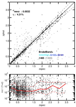
Figure 13.— Comparison between our three tier photometric redshifts vs. spectroscopic redshifts for galaxies with good quality spectroscopic redshift flag in the GOODS-N field. The redshift tier breakdown is approximately 20%, 21% and 59% in tier 3, 2 and 1, respectively. The colors of points and the lines in the bottom pabel have the same meaning as in Figures 11 and 12.

5.1.4 Quality assesment of the photometric redshifts

Figure 11 compares our three tier photometric redshift estimates versus spectroscopic redshifts for galaxies with both G102 and G141 grism spectra and good quality spectroscopic redshifts. Each panel illustrates the gradual improvement in the overall accuracy of the photo-z with the addition of higher spectral resolution data to the SED fit, starting with the broad-band only fits (tier 3, left panel), and progressively including the SHARDS medium bands (tier 2, middle panel), and the grism spectroscopy (tier 1, right panel). The normalized median absolute deviation ($\sigma_{\mathrm{NMAD}}$) of $\Delta z=z_{\mathrm{phot}}-z_{\mathrm{spec}}$, defined as $\sigma_{\mathrm{NMAD}}=1.48\times\mathrm{median}\left(\left|\frac{\Delta z-\textrm{median}(\Delta z)}{1+z_{\mathrm{spec}}}\right|\right)$, improves significantly by a factor of $\sim 10$ and 12 with the use of medium bands and grism spectra, respectively. Similarly, the fraction of outliers, defined as $\eta=\Delta~{}z/(1+z)>0.15$, decreases from 4.2% to 3.3% and 2.7% in those cases. The bottom panels of Figure 11 show the dependence of the $\Delta$z/(1+z) scatter with redshift for the 3 cases. The median value of such scatter corrected by the median offset in $|\Delta z|$ is, by definition, $\sigma_{\mathrm{NMAD}}$. For the tier 3 redshifts, the scatter is relatively constant up to $z\sim 1.5$ and increases by a few percent at higher redshifts. The addition of SHARDS photometry significantly improves the accuracy of the tier 2 redshifts at $z<1.5$ by almost a factor of 7. However, the impact of the medium band data at higher redshifts ($z>1.5$) is almost negligible. This is because the most relevant spectral features (e.g., Balmer or 4000 Å break) shift out of the SHARDS spectral range around that redshift, and thus diminish the constraining effect of the medium-bands. The addition of HST grism spectroscopy does not significantly change the overall $\sigma_{\mathrm{NMAD}}$ accuracy of the redshift with respect to the tier 2 case. Nonetheless, it consistently reduces $\Delta$z/(1+z) to $\sim 0.01\%$ for galaxies with clear emission lines in the redshift range $z=0.4-3$. As a result, the relative improvement of the tier 3 redshifts at low-z is smaller than a factor of 3, but it can increase to almost a factor of 10 for high-z galaxies.

Figure 12 shows the comparison of our photometric redshifts vs. spectroscopic redshifts (left) and vs. the photometric redshifts from the 3D-HST survey (right) which also make use of G141 spectra Momcheva et al. (2016). This comparison is limited to galaxies with G141 spectra in both catalogs and good quality spectroscopic redshifts. The purpose of this comparison is twofold, first showing the relative impact of adding SHARDS medium-band photometry and G102 spectra vs. the G141-only case of 3D-HST, and second, verify that our redshift estimates are consistent with theirs for the galaxies in which the G141 data is the key contributor to the quality PDFz. The redshift dependence on $\Delta$z/(1+z) shown in the bottom panels of Figure 12 indicates that our photometric redshift accuracy is slightly higher at $z\lesssim 0.7$ due to the additional constraints from SHARDS and G102, which are both more effective at picking up emission lines at low-z (see Figure 2). At higher redshifts our estimates are in excellent agreement with those from 3D-HST.

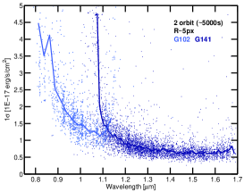
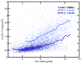
Figure 14.— 1$\sigma$ emission line sensitivity in the G102 and G141 spectra as a function of the observed wavelength (upper panel) and the SExtractor flux_radius size of the galaxies (lower panel). In order to illustrate the effect of the two main drivers of emission line sensitivity separately, the upper panel shows galaxies with similar sizes of $R\sim 5$ pixels, typical for resolved galaxies, while the bottom panel shows galaxies with emission lines measured around the same wavelengths, $\lambda\sim$$1.0~{}\mu$m and $1.5~{}\mu$m for G102 and G141. At those wavelengths, the average line uncertainty of the 2-orbit depth grism spectra for a resolved galaxy are 0.75 and 1.5 $\times 10^{-17}$ erg s^-1 cm^-2 in G141 and G102, respectively.

Note that Figures 11 and 12 include only spectroscopically confirmed sources with clear emission lines. Therefore, the comparisons are biased towards the best possible targets for redshift determination using the HST grisms. This bias consequently boosts the accuracy redshift estimates, i.e., if a galaxy has a confirmed optical emission line it is easier for the NIR grism to pick up another one line in different spectral range thus providing a high precision (0.01% level) redshift estimate. Figure 13 compares photometric and spectroscopic for all galaxies with reliable spectroscopic flag regardless of their HST grism detectability. The number of galaxies in the figure is more than 1.5$\times$ larger than in the previous comparisons and it includes a significant amount of galaxies from tier 2, i.e., galaxies for which the grism spectra do not contribute decisively to the PDFz. Although still biased towards galaxies with emission lines, this comparison provides a more representative estimate of the overall quality of the photometric redshifts for the whole, magnitude limited sample. The accuracy is slightly lower than in the previous comparisons but it is still significantly better than the $\sim$1% precision typical of broad-band only surveys ($\sigma_{\mathrm{NMAD}}$$\sim 0.3\%$ with $\eta\sim 4\%$).

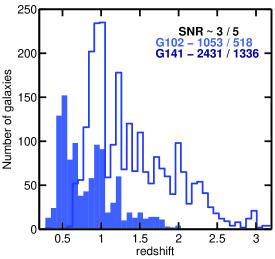
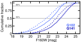
Figure 15.— Top: Redshift histogram for galaxies with clear emission lines (SNR$\geq$3) detected in the G102 (empty light blue) and G141 spectra (filled dark blue). Bottom: Cumulative F160W magnitude distribution for the emission line galaxies in upper panel. The dashed and solid lines indicate the distributions down to SNR$=3$ and 5, respectively.

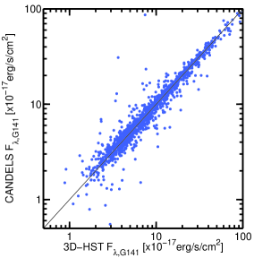
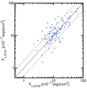
Figure 16.— Left: Comparison of emission line fluxes measured in the G141 spectra by the 3D-HST survey Momcheva et al. (2016) and our measurements in this paper. Both measurements come from the same G141 images but using different source extractions and SED fits to estimate the line redshift and fluxes. The results are in excellent agreement and demonstrate the consistency of the measurements. Right: Comparison of emission line fluxes for galaxies in which the same line (either H$\alpha$ or [OIII]/H$\beta$ can be detected simultaneously in both of our G102 and G141 measurements. This is only possible for a small fraction of the emission line galaxies at narrow redshift ranges around z$\sim 0.7$ (for H$\alpha$) and z$\sim 1.3$ (for [OIII]/H$\beta$).

5.1.5 Breakdown of the photometric redshift tiers

Since the quality of the photometric redshifts depends on the data used for the SED fit it is useful to report the relative fractions of galaxies in the sample that have observations in each of the relevant datasets or photo-z tiers discussed in the previous sections. In terms of area coverage, approximately $\sim$80% of the CANDELS F160W mosaic is covered by the SHARDS medium band imaging, and an additional $\sim$3% of the non-SHARDS area is covered by the WFC3 G102 and/or G141 mosaics. Thus less than $\sim$20% of all galaxies have tier 3 redshifts, i.e., based on broad-band photometry only. Among the 80% of the sample with SHARDS observations, the relative fraction of galaxies with tier 2 and tier 1 redshifts, i.e., the fraction of galaxies with both SHARDS photometry and HST grism spectra is magnitude dependent. For a magnitude limit of H$<24$ mag, the breakdown is 26% and 74% in tiers 2 and 1, and 35% and 65% for $H<25$ mag. Relative to the whole catalog, these numbers imply that 60% and 52% of all galaxies have tier 1 redshifts at H$<24$ and 25 mag, respectively.

For the galaxies with observations in both grisms, the SED fitting procedure combines the G102 and G141 spectra for the redshift determinations. However, given the lower sensitivity of the G102 grism (see next section for more details) some galaxies might only have G141 detections. For galaxies detected in at least one of the grisms and a magnitude limit of H$<24$ mag, the breakdown between galaxies with both G141 and G102 spectra vs. only G141 spectra is approximately 55% to 33%. The remaining 12% of the galaxies have only G102 observations. The latter are typically located in a region with G141 coverage, however, differences in the orientation of the G102 and G141 observations can make the G141 spectra unavailable or severely contaminated.

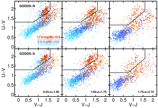
Figure 17.— Rest-frame UVJ diagram for galaxies in the deepest CANDELS fields, GOODS-N (this paper) and GOODS-S (from Guo et al. 2013). Each column presents the rest-frame colors for galaxies in the two fields at the same redshifts, with redshift increasing from left to right. The diagram is color-coded by mass, with the lowest mass galaxies in blue and the highest mass galaxies in red, as shown by the legend in the upper-left panel. The black lines indicate the selection box used to separate quiescent from star-forming galaxies, based on Williams et al. (2009).

5.2. G102/G141 Emission line fits

We compute emission line fluxes and observed-frame equivalent widths from the G102 and G141 spectra using the same software described in the 3D-HST survey paper Momcheva et al. (2016). Briefly, this code adopts the 2D continuum template determined from photometric redshift fit to build a 2D model and then adds Gaussian lines with unresolved line widths of $\sigma=100$ km/s. Each potential line is treated separately by means of independent line-template normalizations relative to the continuum. The code fits the observed grism data to the model using the emcee sampler (Foreman-Mackey et al. 2013) to determine the marginalized posterior distribution functions of the parameters for the individual line-template normalizations. These are converted directly to line fluxes and observed-frame equivalent widths in physical units (i.e., $\mathrm{erg}~{}\mathrm{s}^{-1}~{}\mathrm{cm}^{-2}$ and Å, respectively). Only the lines that fall within the rest-frame spectral range of the grism data, as determined from the grism redshifts, are included in the model (see Table 4 of Momcheva et al. 2016 for a complete list of all the species included in the fit). The line fluxes are implicitly normalized to the total broad band photometry, as the spectra are scaled to match the photometric data. Note that the line-template normalization is not required to be positive, and therefore it is not restricted to measure emission lines, i.e., it can also provide equivalent width estimates for absorption lines.

The MCMC chains provide a robust estimate of the uncertainties in the fit, which are primarily determined by two effects: 1) the wavelength dependence of the grism throughput, and 2) the galaxy size (i.e., the area of the effective aperture of the 2D spectrum fit). Figure 14 illustrates these two effects separately for the G102 and G141 spectra. The top panel depicts the wavelength dependence of the sensitivity for sources with SExtractor FLUX_RADIUS$=3-5$ pixels while the bottom panel depicts the dependence on the galaxy size at the peak sensitivity wavelength of each grism. Overall, a typical resolved galaxy exhibits a 1$\sigma$ flux uncertainty of $\sim 1.5\times 10^{-17}$erg s^-1 cm^-2 in G102 and $\sim 0.8\times 10^{-17}$erg s^-1 cm^-2 in G141 for 2-orbit depth exposures. The lower sensitivity threshold of the G102 grism compared to G141 is largely due to its higher spectral resolution (i.e., the line flux spreads over more pixels and thus reaches a lower the S/N per resolution element for similar exposure times). The noise levels are in good agreement with previously published sensitivities of the HST NIR grisms (e.g., Atek et al. 2010; Brammer et al. 2012; Trump et al. 2013; Treu et al. 2015).

Figure 15 shows the redshift distribution and the cumulative fraction as a function of magnitude for emission line galaxies detected in the G102 and G141 spectra. The lower sensitivity of the G102 grism results in approximately half the number of emission line detections as in G141 at SNR $\gtrsim 3$ or 5. Furthermore, its bluer central wavelength implies that the majority of those detections in G102 have lower median redshifts than those in G141. As indicated in Figure 2, the bluest of the most prominent emission lines, [Oii], shifts out of the G102 spectral coverage at $z\sim 2$, while it can be detected in G141 up to $z\sim 3.5$. This is consistent with the distributions shown in the histograms of Figure 15. The overall brighter magnitudes of the emission line galaxies detected in G102 implies that the majority of those galaxies are also detected in G141 for redshifts $z\gtrsim 0.6$ (i.e., when the H$\alpha$ line shifts into the G141 passband). This naturally provides simultaneous detections of two relevant lines in the combined dataset, for example H$\alpha$ and H$\beta$ at $z=0.6-1.3$, or [OIII] and [OII] at $z=1.3-2.0$. The majority ($>90\%$) of the G102 emission line detections with SNR $\geq$3 (5) have magnitudes $H\leq 23.5$ (23), while the G141 detections are about 1 magnitude fainter with SNR $\geq 3$ (5) at H $\leq$ 24.5 (24). Relative to the full galaxy catalog, these numbers imply that $\sim$25% of the galaxies with $H<24.5$ have at least one emission line detected in the G141 grism, and $\sim$35% of the galaxies with $H<23.5$ have two emission lines detected, one on each of the G102 and G141 grisms.

In order to validate the quality of the emission line extractions, we compare the line fluxes measured in the G141 grism to those released by the 3D-HST survey in Momcheva et al. (2016). Note that while we make use of the reduced G141 images released by the 3D-HST survey, the 2D extraction of the spectra, the redshift determination and the line measurements depend on our object detection procedure and on our SEDs. Therefore, this is a useful quality check to verify that our extraction and SED fitting procedures are accurate. This comparison is shown in the left panel of Figure 16, which illustrates that the fluxes from both catalogs are in excellent agreement even for the faintest emission lines with f${}_{\lambda}\sim 1\times 10^{-17}$erg s^-1 cm^-2 which have low SNR $\lesssim 3$.

The right panel of Figure 16 extends this validation test to the emission lines detected in G102 by comparing the flux measurements for emission lines that are simultaneously detected in both G102 and G141. This is only possible for a small sub-sample of galaxies in narrow redshift ranges where the most prominent lines lie in the reddest and the bluest sides of the G102 and G141 wavelength ranges, respectively ($z\sim 0.7$ for H$\alpha$, and $z\sim 1.3$ for [OIII]/H$\beta$). In this case the comparison is between fully independent measurements performed in different datasets, and we also find a good agreement for all the emission lines with SNR$\gtrsim 3$. The scatter is consistent with the $\sim 1.5\times$ dispersion reported in Momcheva et al. (2016) for the comparison between grism and ground-based spectroscopic measurements. Note also that, in order to measure the same line in both grisms, the fluxes are typically measured near the edges of the spectra, around $\lambda_{\rm obs}\sim 1.1\mu$m, where the sensitivities are lower (see Figure 14).

5.3. Rest-frame colors and stellar population properties

We compute stellar population properties and rest-frame luminosities by fitting the observed SEDs to galaxy templates and adopting the best photometric redshift. We used the best available SED for every galaxy including broad- and medium- band photometry, but not the grism spectroscopy. First, we estimate stellar masses and other physical properties of the galaxies, such as stellar ages, dust extinctions or SFRs by fitting the SEDs with the codes FAST (Kriek et al. 2009) and Synthesizer (Pérez-González et al. 2005, 2008). The redshift is fixed to best redshift estimate, i.e., spectroscopic where available and photometric otherwise. The modeling assumptions for both codes are as follows: we use the Bruzual & Charlot (2003) stellar population synthesis models with a Chabrier (2003) IMF and solar metallicity. We assume exponentially declining star formation histories with a minimum e-folding time of $\log_{10}(\tau/yr)=8.5$, a minimum age of 40 Myr, $0<A_{V}<4$ mag and the Calzetti et al. (2000) dust attenuation law. The only difference between the FAST and Synthesizer fits is that the latter uses SED templates that include emission lines. In addition to the stellar population properties, we also estimate rest-frame luminosities and colors for all galaxies using EAZY (Brammer et al. 2008). This code computes the rest-frame luminosity in a set of typical photometric filters (see Table B3), and then derives rest-frame colors as the ratio of the luminosities in two of those filters.

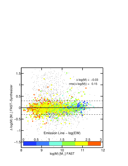
Figure 18.— Comparison of the stellar masses computed using FAST and Synthesizer with the same modeling assumptions (see text). The primary difference between the galaxy models is that Synthesizer includes emission lines in the SEDs. The stellar mass estimates are fully consistent. The overall distribution is centered around zero with a scatter of $0.15$ dex. We find no systematic affects the stellar masses of galaxies with strong emission lines, identified using the WFC3 grism spectra. The color code indicates the EW of the H$\alpha$ and [Oiii]emission lines in those galaxies.

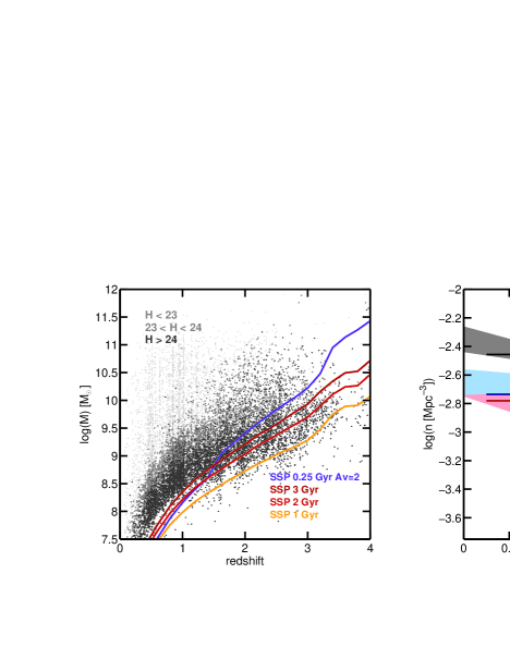
Figure 19.— Left: Galaxy stellar masses as a function of redshift for the CANDELS GOODS-N sample with a grey-color intensity scale for the H-band magnitude. We estimate the stellar mass completeness of the sample by showing the stellar mass threshold for a series of intrinsically red, quiescent or dusty (orange, red and purple lines), galaxy templates with an observed H-band magnitude equal to the SNR$\sim$5 detection limit of the catalog, H$\sim$26. Right: Comoving number density for galaxies more massive than log(M/M_⊙)$>10$ divided in three groups, star forming (blue), quiescent (red) and both together (black), and compared to the results from the ULTRAVISTA COSMOS sample for the same range in stellar mass (shaded regions). The catalog provides results which are consistent with the literature (Muzzin et al. 2013) indicating that both our stellar masses and rest-frame colors are robust.

Figure 17 illustrates the consistency of these rest-frame colors by comparing the distribution of galaxies in the UVJ color-color diagrams (Williams et al. 2009) based on the CANDELS/GOODS-N catalog and the CANDELS/GOODS-S catalog of Guo et al. (2013) (i.e., the deepest CANDELS fields) in 3 redshift bins. The color distributions are qualitatively very similar and they are also consistent with the UVJ diagram for the 3D-HST sample (Figure 26 of Brammer et al. 2012). The mass distribution in the color-color diagram is also consistent with previous results which showed that the majority of massive galaxies at $z\gtrsim 1$ tend to be intrinsically red ($U-V$), either because of dust obscuration of because they host older stellar populations (Brammer et al. 2011). The UVJ diagram is indeed particularly useful to make this distinction because it breaks the degeneracy between the dusty star-forming galaxies and quiescent galaxies with low levels of star formation. Both the old and the dusty populations have red $U-V$ colors (upper left region), but dusty star-forming galaxies typically have redder $V-J$ colors (e.g., Whitaker et al. 2012). The black lines indicate the selection threshold that is typically used to distinguish these two populations. In the following we adopt the UVJ criterion to divide the GOODS-N sample in star-forming and quiescent galaxies at all redshifts. We validate the accuracy of this selection criterion by comparing the evolution in the number densities of these two populations to the results from previous works (see below).

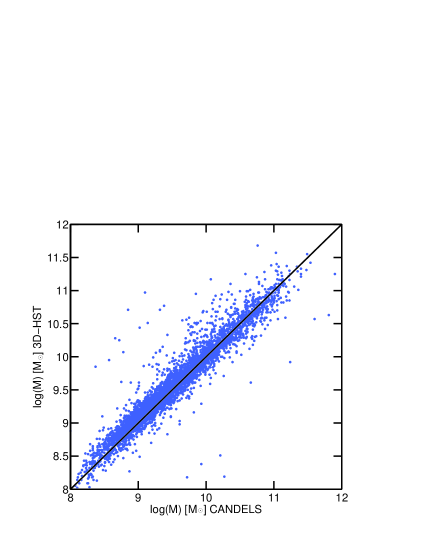
Figure 20.— Stellar mass comparison for the galaxies in the GOODS-N CANDELS and 3D-HST catalogs. Both sets of stellar masses are consistent with each other showing almost negligible offsets, $\Delta$log(M/M_⊙) $<0.03$ dex, and a scatter of $\sim$0.3 dex, typical of the SED fit based stellar mass estimates.

Figure 18 shows the comparison of the stellar masses computed with FAST and Synthesizer. The overall difference between these estimates for the whole galaxy sample is consistent with zero within the usual scatter of $\sim 0.3$ dex typical of the comparison of stellar masses derived with different codes (e.g., Mobasher et al. 2015, Nayyeri et al. 2017). Furthermore, we find no obvious systematic differences in the stellar masses of galaxies with strong, high EW emission lines, identified in the G102 and G141 spectra (H$\alpha$ or [Oiii]; colored circles), as a result of using galaxy templates with or without emission lines in the SED fitting procedure. Nonetheless, we release with this paper the best-fit SEDs computed with both FAST and Synthesizer to enable further investigations in specific subsets of emission line galaxies. Since there are no obvious advantages to the use of either set of stellar mass estimates we choose the values computed with FAST as our fiducial stellar masses for the remainder of this work. This choice allows a more direct comparison to the stellar masses computed by the 3D-HST survey using the same fitting code and modeling assumptions (see below).

The left panel of Figure 19 shows the stellar mass distribution for all galaxies in our catalog as a function of redshift using a grey-color intensity scale to indicate the H-band magnitude of the galaxies. We use this diagram to study the mass completeness of the sample. The completeness of magnitude limited samples, such as this one, decreases with redshift and is typically lower for red galaxies, either because they have intrinsically old stellar populations with larger mass-to-light ratios, or because the dust attenuation makes the galaxies fainter than unobscured SFGs of the same mass. Therefore, we characterize the mass completeness of the sample by estimating the mass threshold for the reddest galaxies with H-band magnitudes equal to the SNR$\sim$5 detection limit of the survey ($H\sim 26$). Red galaxies fainter than this threshold will be undetected at the depth of the survey. The orange and red lines show the mass completeness limit for 3 galaxy templates of quiescent galaxies with ages ranging between $1-3$ Gyr, i.e., the age of a recently quenched galaxy at any redshift, and the age of maximally old galaxies at $z=2-3$. The purple line shows the detection limit for a young (250 Myr), dusty (Av$=2$) star-forming galaxy. In agreement with previous estimates of the mass completeness for the CANDELS catalogs in other fields (e.g., Tal et al. 2014; Nayyeri et al. 2017; Stefanon et al. 2017), we find that our catalog is complete to log(M/M_⊙)$\gtrsim 10$ up to redshift $z\sim 3$ except perhaps for the most extreme dusty galaxies (Av$\gg 2$; see e.g., Wang et al. 2016 for a study of dusty H-band drop outs). Interestingly, massive, recently quenched galaxies (also called post-starburst) can be reliably detected up to $z\sim 4$, as shown for example in Straatman et al. 2014.

We further verify the quality of the stellar mass estimates by studying the comoving number density of massive (log(M/M_⊙)$>$ 10) star-forming and quiescent galaxies as a function of redshift. The right panel of Figure 19 shows that these number densities agree with the results from the ULTRAVISTA sample (Muzzin et al. 2013), which covers a larger area but to a shallower depth, at the same redshifts and follow the predicted trend at higher z. The CANDELS/GOODS-N sample is likely more susceptible to cosmic variance effects at the lowest redshift bin, but owing to its deeper limiting magnitude, it is possible to follow the evolution of both blue and red galaxies up to higher redshifts. Figure 20 shows one last quality check which compares our stellar mass estimates vs. those from 3D-HST catalog for the same galaxies. We find that the average offset, and the scatter are in excellent agreement as reported in similar comparisons presented in previous CANDELS data papers for the other 4 fields.

Figure 21.— Example of a UV-to-FIR SEDs. The black line shows best-fit BC03 stellar population model for the photometry up to 8$\mu$m rest-frame (open black stars), which provide an estimate of the stellar population properties and the dust attenuation. The filled balck stars show the mid-to-far IR data from Spitzer MIPS and Herschel PACS and SPIRE. The red, green, blue and cyan lines show the best-fit dust emission models from the libraries of Chary & Elbaz (2001), Dale & Helou (2002), Rieke et al. (2009) and Draine & Li (2007), which provide similar results. The dashed line shows the fit to only the MIPS 24 $\mu$m data. The significant difference between this and the other templates illustrates why using an average luminosity template, as in the (Wuyts et al. 2011b) method, is a better approach for MIPS only SEDs.

Figure 22.— Comparison between different total SFR indicators at different redshifts. The x-axis show the SFRs derived from the combination of the observed (unobscured) UV SFR${}_{\rm UV}^{\rm obs}$ and the IR-based SFR determined from the MIPS 24 $\mu$m flux using the prescription of Wuyts et al. (2011b), SFR${}_{\rm IR}^{\rm W11}$. They y-axis shows the total SFR derived either from the UV luminosity, corrected for extinction (SFR${}_{\rm UV}^{\rm corr}$; grey circles), or the combination of SFR${}_{\rm UV}^{\rm obs}$ and the IR-based SFRs computed from the fit of all the available FIR data to dust emission templates (red circles). The median difference between SFR estimates, $\Delta\log$SFR, is indicated for the UV corrected (black) and IR-based (red) SFRs. Overall, the two different estimates exhibit a good agreement showing that is it possible to combine them in a SFR ladder, that spans a range of more than 2 dex in SFRs.

5.4. UV+IR SFRs

5.4.1 The “ladder” of SFR indicators

In this section we use the UV-to-FIR SEDs to provide SFR estimates for the galaxies in the sample. The depth of the optical/NIR photometry guarantees accurate measurements of the rest-frame UV emission ($\lambda\sim 1500-2500$ Å), which is an excellent tracer of the ongoing star formation, for all galaxies up to the highest redshifts. However, the ubiquitous presence of dust in star forming galaxies, typically embedded in the same gas from which stars are formed, implies that the intrinsic UV emission of the galaxies if frequently attenuated by dust absorption. In galaxies with low-to-mid attenuations, it is possible to correct for the effect of dust absorption using different methods such as the slope of the UV emission, which is correlated with the Av (e.g.; Meurer et al. 1997), or by estimating such Av from the optical-to-NIR SED fitting to stellar population models, which provides also a direct estimate of the intrinsic SFR. Nonetheless, several works have shown that the strong dust attenuations found in massive galaxies at $z\gtrsim 1.5$ can bias these corrections downwards, thus underestimating the SFRs (e.g., Daddi et al. 2007; Reddy et al. 2008, 2010; Wuyts et al. 2011a). The availability of FIR photometry provides a direct probe into the emission of the dust particles, responsible for the optical attenuation, which are being heated by the UV photons and re-radiate this energy at longer wavelengths. Hence the FIR photometry provides a useful SFR indicator for severely obscured galaxies, which make a significant fraction of the massive galaxy population at high z. The main drawback of this method is that the shallower depth of the IR observations, compared to the optical and NIR data, limits the SFR detection threshold, which becomes increasingly higher with redshift and eventually leads to incompleteness even at the high mass end (see e.g., Figure 2 of Scoville et al. 2016).

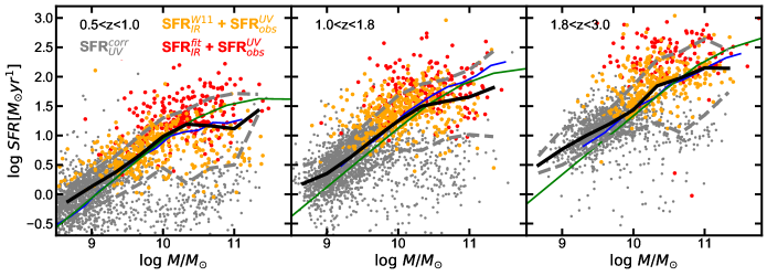
Figure 23.— SFR vs. stellar mass diagram (i.e., the SFR sequence; Noeske et al. 2007) as a function of redshift compared to results from the literature. The SFRs in the y-axis are computed by combining the different SFR indicators in Figure 22 (grey, orange and red circles) to assemble the SFR ladder. The black and grey lines show the running median and 1$\sigma$ scatter of the star forming galaxies identified with the UVJ criterion. The blue and green lines show the SFR sequence from Whitaker et al. (2014) and Schreiber et al. (2015a) which are roughly consistent with the overall distributions at all redshifts.

A way forward to overcome the issues in both the UV and IR based SFR estimates is to combine the constraints coming from both methods by using a ladder of SFR indicators that can be cross-calibrated on relatively massive galaxies with intermediate dust attenuations and low IR fluxes. Here we follow such approach by using a method similar to the one described in Wuyts et al. (2011a). Briefly, the SFR ladder usually consists of three steps which differ on the amount of SFR indicators that are available for each galaxy, namely, UV, which is availabe for all galaxies, mid-IR, available only for a subset of massive (log(M/M_⊙)$\gtrsim$10) up to $z\sim 3$, and far IR, available only for a subset of those mid-IR detected galaxies.

The first step of the ladder is a UV-based SFR derived from the rest-frame UV luminosities of the galaxies. Owing to the breadth of optical and NIR photometric data the rest-frame UV luminosity (i.e., the monochromatic luminosity at 280 nm) can be measured for galaxies at $z\gtrsim 0.3$. Thus, it provides a general, homogeneous SFR estimate for the whole sample. To compute the SFR from the UV luminosity, we use the relation of Kennicutt (1998), applying a correction for dust attenuation, SFR${}_{\rm TOT}(M_{\odot}~{}\rm yr^{-1})=SFR_{\rm UV}^{\rm corr}=1.09\times 10^{-10}\times 10^{0.4*A_{UV}}[3.3~{}L_{\rm UV}(280)/L_{\odot}]$, where $L(280)$ and A_UV are the UV luminosity and dust attenuation at $\lambda=280$ nm, respectively. The UV attenuation can be inferred directly from the the best-fit model to the overall SED, which assumes a Calzetti et al. (2000) attenuation law (i.e., A_UV=A(280)=1.8Av). However, rather than assuming these values, here we estimate $A_{\rm UV}$ on a galaxy-by-galaxy basis from the comparison of the slope of the UV continuum emission ($\beta$; $f_{\lambda}\propto\lambda^{\beta}$) to the ratio of UV to IR luminosities ($L(8-1000)/L_{\rm UV}\equiv$IRX), or upper limits of the latter. The IRX-$\beta$ diagram provides a useful diagnostic to characterize the dust attenution in each galaxy (Meurer et al. 1997; Kong et al. 2004; Buat et al. 2007). This is particularly relevant to avoid overestimating the dust attenuation in blue, low mass galaxies, undetected in the IR, for which the starburst like Calzetti et al. (2000) attenuation law is not a good match. A more detailed description of this method is presented in appendix D.

The second and third steps of the SFR ladder include only galaxies with mid-to-far IR detections. For those galaxies, we use a hybrid estimate that combines UV and IR tracers. Firstly, we estimate the contribution of the dust obscured SFR by fitting the FIR SEDs with dust emission templates (see next section) and computing the integrated IR luminosity, from 8 to 1000 $\mu$m, L(8-1000). Then, we obtain the total SFR by adding the contributions from the obscured (IR) and the observed, unobscured (UV) SFR, SFR${}_{\rm TOT}=~{}$SFR${}_{\rm IR}+$SFR${}_{\rm UV}^{\mathrm{obs}}$ (e.g., Kennicutt 1998; Bell et al. 2005),

$${\rm SFR}_{\rm TOT}=1.09\times 10^{-10}[L(8-1000)+3.3~{}L_{\rm UV}(280)]$$ (1)

where SFR is given in $\mathrm{M_{\odot}\,yr^{-1}}$, the luminosities are in L_⊙ and the conversion factor from luminosity to SFR assumes a Chabrier (2003) IMF.

5.4.2 Mid and far IR based SFR

For galaxies with IR detections we distinguish between those with only mid-IR detections and those with both mid- and far- IR detections. As discussed in Section 2, our catalog includes photometry both from Spitzer and Herschel. The Spitzer/MIPS 24 $\mu$m photometry is deeper than Herschel PACS and it has higher spatial resolution than that of SPIRE. The downside of MIPS, is that it probes shorter, mid-IR wavelengths, whereas the Herschel data spans a broader, FIR wavelength range from $\lambda=100-500$ $\mu$m. Nonetheless, owing to its depth, a larger fraction of the sample is detected at 24 $\mu$m than in any Herschel band and thus provides SFR estimates for a large fraction of the massive galaxies up to $z\sim 3$. For galaxies detected only in MIPS 24 $\mu$m, the modeling of the FIR emission with dust templates is uncertain, as it is only constrained by one point, and it is prone to overestimate the SFR at high-z due to a bias towards ULIRG templates for relatively normal galaxies (Daddi et al. 2007; Symeonidis et al. 2008; Kartaltepe et al. 2010; Barro et al. 2011; Elbaz et al. 2011). In order to avoid this problem, we use the analytic conversion from MIPS 24 $\mu$m fluxes to L(TIR) from Wuyts et al. (2008, 2011b), SFR${}_{\rm IR}^{\rm W11}$. This calibration uses only one template generated by averaging multiple dust emission templates and comparing to stacked Spitzer and Herschel photometry for multiple galaxies (see also Rieke et al. 2009 or Rujopakarn et al. 2013 for similar calibrations).

For galaxies with detections in multiple FIR photometric bands (e.g., galaxy SED in Figure 21), we fit the thermal IR emission (those bands redder than 5 $\mu$m rest-frame, which are supposed to be dominated by dust emission) to the templates from the libraries of Chary & Elbaz (2001), Dale & Helou (2002), Rieke et al. (2009) and Draine & Li (2007). Then, we compute the integrated luminosity L(TIR) as the average value of the four sets. The typical differences in the predictions from the different models are roughly a factor 2, consistent with the typical uncertainties in similar kind of studies (Papovich et al. 2006, Daddi et al. 2007, Magnelli et al. 2009), SFR${}_{\rm IR}^{\rm fit}$. We also compute L(TIR) using the Wuyts et al. (2008) formula for these galaxies to have an additional estimate of the SFR that can be used to validate the accuracy of the IR SED fitting.

5.4.3 Comparison of the SFRs

Following Wuyts et al. 2011b, we cross compare the different SFR estimates to validate their accuracy and consistency. Figure 22 shows the comparison between the total SFR based on the UV luminosity, corrected for extinction (SFR${}_{\rm UV}^{\rm corr}$; grey), and the total SFR determined from the fitting of all the far IR data to dust emission templates (SFR${}_{\rm IR}^{\rm fit}$+SFR${}_{\rm UV}^{\rm obs}$; red) vs. the total SFR based on the MIPS 24 $\mu$m fluxes and the Wuyts et al. (2011b) relation (SFR${}_{\rm IR}^{\rm W11}$+SFR${}_{\rm UV}^{\rm obs}$). The comparison to SFR${}_{\rm UV}^{\rm corr}$ is based on galaxies with relatively weak MIPS detections, f(24$\mu$m)$>20-150$ $\mu$Jy, while the comparison to the IR SED-fitting SFRs includes all galaxies with at least one detection in a Herschel band. Overall, both comparisons are in qualitatively good agreement showing that the SFR ladder method can be used to derive self-consistent SFRs across a wide range of galaxy masses and redshifts. The comparison to SFR${}_{\rm UV}^{\rm corr}$ shows a small offset and scatter, $\Delta$SFR$\sim 0.03\pm 0.32$ dex, that are consistent with the typical dispersion expected in this kind of comparisons ($\sim 0.3$ dex; e.g., Wuyts et al. 2011b). The comparison between the two IR-based SFRs shows a similar offset but a much smaller scatter ($\lesssim$0.02$\pm 0.17$ dex). The excellent agreement for the latter is not surprising, considering that the MIPS data is used in both SFR estimates, whereas the comparison to the UV-corrected SFRs is based on completely different tracers (UV vs. IR).

We further analyze the consistency of the SFR ladder by comparing the locus of our SFR main sequence, i.e., the correlation between SFR and stellar mass (e.g., Noeske et al. 2007; Elbaz et al. 2011; Whitaker et al. 2014), at different redshifts, with previous results from the literature. Figure 23 shows how the combination of the different tiers of the SFR ladder (grey, orange and red circles) reproduce the characteristic distribution of the SFR sequence, which exhibits a slope close to unity at lower masses, and flattens towards the high-mass end (e.g., Speagle et al. 2014). The black and grey lines show the running median and 1$\sigma$ scatter of the distribution for star-forming galaxies selected using the UVJ diagram (see figure 17). The overall distribution exhibits a good agreement with the results of Whitaker et al. (2014, blue line) and Schreiber et al. (2015a, green line), also based on far-IR photometry, and shows a similar curvature as a function of mass. We further discuss the properties of the SFR main sequence derived from our SFR estimates in appendix D, which also expands the analysis to include data from the 5 CANDELS fields.

6. Summary

In this paper we present an HST/WFC3 F160W (H-band) selected sample in the CANDELS/GOODS-N field characterized with UV-to-FIR SEDs. The sources are selected from an F160W mosaic which combines data from the deep and wide observations of the CANDELS program over a total area of 171 arcmin². The photometric catalog includes the newly observed HST data in F105W, F125W, and F160W, taken as part of the CANDELS survey, with all the previous HST optical observations in ACS F435W, F606W, F775W, F814W, and F850LP from GOODS and other smaller programs. In addition to the HST data we include deep photometric data in 25 optical medium-band filters from the SHARDS survey (Pérez-González et al. 2013), which constitutes one of the deepest ($i$-band $\sim 28$ mag) and highest resolution (R$\sim$50) medium-band surveys, surpassing the depth, spectral coverage and resolution of similar medium band observations in other deep fields such as COSMOS or GOODS-S. Furthermore, we include ancillary data in the ultraviolet: LBC/U and KPNO/U’, near IR: MOIRCS/K, CFHT/K’ and Spitzer/IRAC 3.6, 4.5, 5.8, 8.0 $\mu$m and a wealth of far IR photometry at 24 $\mu$m, and 70 $\mu$m  from Spitzer MIPS and at 100 $\mu$m, 160 $\mu$m, 250 $\mu$m, 350 $\mu$m, and 500 $\mu$m, from Herschel PACS and SPIRE. In addition, we complement and expand the broad and medium band photometry with WFC3/IR grism spectroscopy in G102, from new observations (GO:13179), and in G141 from AGHAST (GO:11600), as reduced by 3D-HST (Momcheva et al. 2016). The combined grism observations make GOODS-N the first among the deep cosmological fields to have similar areal coverage in the contiguous grisms, which enables a simultaneous analysis of several emission lines at different redshifts.

As in previous CANDELS papers, the source detection is based on a slightly modified version of SExtractor which runs and combines the output of two configurations (“cold” and “hot”) to optimally detect and extract all sources ranging from the largest, most extended, and brightest ones to the faintest and smallest. Similarly, we use TFIT to measure uniform multi-band photometry in the lower resolution optical-to-NIR bands. TFIT uses priors from the positions of the F160W detections to construct object templates that are PSF-matched and fitted to the low-resolution images to measure the photometry. The FIR photometry is measured independently and self-consistently on the Spitzerand Herschel images using MIPS 24$\mu$m priors. Then, each IR source is assigned a single F160W counterpart based on coordinates and IRAC fluxes. The F160W-selected catalog contains $>$35,000 sources down to a 5$\sigma$ limiting depth of $H=$27.4 and 28.2 mag in the wide and deep regions of the mosaic, respectively.

We show that the overall SEDs present the level of consistency required to characterize the intrinsic stellar populations of the galaxy, and we perform a galaxy-by-galaxy fitting of the UV-to-FIR SEDs to stellar population and dust emission models and a fit of their grism spectra for emission and absorption lines. From the best fitting optical and IR templates, we estimate: (1) photometric redshifts, (2) stellar population properties (i.e., stellar masses, Av, etc.) and (3) SFRs. From the line-fitting of the G102 and G141 HST grism data, we estimate line fluxes and equivalent widths. Then, we analyze the accuracy and reliability of these estimates with respect to different parameters. A summary of the most important results of this analysis follows.

• The use of medium-band photometry and grism spectroscopy significantly improves the quality of the photometric redshifts relative to the case of SED fitting to broad-band photometry only. The comparison to 1,485 spectroscopic redshifts up to $z\sim 3$ yields a $\sigma_{\rm NCMAD}=0.0032$ and an outlier fraction of $\eta=$4.3%, nearly a factor of 7 more precise than the typical, broad-band based redshifts.

• Owing to the deep limiting magnitude of the F160W mosaic, our catalog is nearly complete for stellar masses above log(M/M_⊙)$=10$ up to redshift $z\sim 3$, except perhaps for the most extreme dusty galaxies (Av$\gg$2).

• The line catalog contains nearly 2,000 emission lines detected at SNR$>3$, with 30% and 70% of them identified in the G102 and G141 spectra, respectively. The G102 detections are typically in brighter and lower redshift galaxies, $H<23.5$ and $\bar{z}=0.7$, while the G141 detections are in fainter and higher redshfit galaxies, $H<24.5$ and $\bar{z}=1.5$. For magnitudes $H<23.5$, roughly 35% of all galaxies have two emission lines detected, typically H$\alpha$(G141) and H$\beta$(G102) at $z=0.6-1.3$.

• We obtain robust SFRs for all the galaxies in the catalog by using in each case the best available SFR tracer from either the rest-frame UV or the far IR emission. The overall SFR ladder is computed self-consistently verifying the consistency in the SFRs for galaxies with multiple indicators, and showing that the resulting SFR main sequence is in good agreement with previous works at all redshifts over a range of 2 dex in stellar mass.

The multi-band photometry and the added-value catalogs (see appendices) presented in this paper are further complemented with additional data products from the CANDELS survey which allow even richer studies the galaxy populations by adding, for example, structural properties (van der Wel et al. 2014) or visual morphologies (Huertas-Company et al. 2015), which enables a wide array of additional science in one of the premier cosmological fields.

Appendix A Photometric catalogs

This appendix features CANDELS GOODS-N multi-band photometric catalog entries with optical observations from KPNO, LBC, HST/ACS, near infrared data from HST/ WFC3, CFHT and Subaru, and infrared observations from Spitzer/IRAC (Table A1). This catalog also contains useful SExtractor outputs for the HST bands as in the catalogs released with the previous CANDELS papers.

Table A1Description of the CANDELS GOODS-N Photometric Catalog

Column No. Column Title Description 1 ID Object identifier, beginning from 1 2 IAU Name 3,4 RA, DEC Right ascension and declination (J2000.0; decimal degrees) 5 FLAGS SExtractor F160W flag used to designate suspicious sources that fall in contaminated regions 6 CLASS_STAR SExtractor CLASS_STAR parameter in the F160W band 7 X-ray X-ray ID from Alexander et al. (2003) 8–41 Flux, Flux_Err Flux and flux in each filter. Sources that are not observed have (-99.00, -99.00, 0). Filters are included in order: KPNO_U, LBC_U, F435W, F606W, F775W, F814W, F850LP, F105W, F125W, F160W, MOIRCS_Ks, CFHT_Ks, 3.6 $\mu$m, 4.5 $\mu$m, 5.8 $\mu$m, and 8.0 $\mu$m 1 ID Object identifier, beginning from 1 2–10 FLUX_MAX in HST bands 11–28 FLUX_ISO, FLUXERR_ISO Isophotal flux and flux error in 9 HST bands 29–46 FLUX_ISOCOR, FLUXERR_ISOCOR Isophotal flux and flux error in 9 HST bands 47–64 FLUX_AUTO, FLUXERR_AUTO AUTO flux and flux error in HST 9 bands 65–82 FLUX_PETRO, FLUXERR_PETRO PETRO flux and flux error in HST 9 bands 83–100 FLUX_BEST, FLUXERR_BEST BEST flux and flux error in HST 9 bands 101–280 FLUX_APER, FLUXERR_APER APER flux and flux error in HST 9 bands and 10 circular apertures of radius 1.47, 2.08, 2.94, 4.17, 5.88, 8.34, 11.79, 16.66, 23.57, 33.34, 47.13 1 ID Object identifier, beginning from 1 2 X_IMAGE Object position along x [pixel] 3 Y_IMAGE Object position along y [pixel] 4 XPEAK_IMAGE x-coordinate of the brightest pixel [pixel] 5 YPEAK_IMAGE y-coordinate of the brightest pixel [pixel] 6 XMIN_IMAGE Minimum x-coordinate among detected pixels [pixel] 7 YMIN_IMAGE Minimum y-coordinate among detected pixels [pixel] 8 XMAX_IMAGE Maximum x-coordinate among detected pixels [pixel] 9 YMAX_IMAGE Maximum y-coordinate among detected pixels [pixel] 10 X2_IMAGE Variance along x [pixel**2] 11 Y2_IMAGE Variance along y [pixel**2] 12 XY_IMAGE Covariance between x and y [pixel**2] 13 CXX_IMAGE Cxx object ellipse parameter [pixel**(-2)] 14 CYY_IMAGE Cyy object ellipse parameter [pixel**(-2)] 15 CXY_IMAGE Cxy object ellipse parameter [pixel**(-2)] 16,17 A_IMAGE, B_IMAGE F160W profile RMS along major and minor axis (pixel) 18,19 ERRA_IMAGE, ERRB_IMAGE F160W profile RMS along major and minor axis (pixel) 20,21 THETA_IMAGE, ERRTHETA_IMAGE F160W position angle (degree) 22 ISOAREAF_IMAGE SExtractor F160W Isophotal area (filtered) above Detection threshold (${\rm pixel^{2}}$) 23–31 ISOAREA_IMAGE SExtractor Isophotal area (filtered) above Detection threshold (${\rm pixel^{2}}$) in HST bands 32–40 BACKGROUND Background at centroid position in HST bands 41–49 FLUX_RADIUS_1 RADIUS_1 with the 0.2 fraction of light in HST bands 50–58 FLUX_RADIUS_2 RADIUS_2 with the 0.5 fraction of light in HST bands 59–67 FLUX_RADIUS_3 RADIUS_3 with the 0.8 fraction of light in HST bands 68–76 FWHM_IMAGE FWHM of the image of an object, in unit of pixel (1 pixel = 0$\farcs$06) in HST bands 77 KRON_RADIUS F160W band Kron radius from SExtractor (in unit of A_IMAGE or B_IMAGE) 78 PETRO_RADIUS F160W band Petrosian radius from SExtractor (in unit of A_IMAGE or B_IMAGE)

A separated catalog containing the photometry in the 25 medium bands of the SHARDS survey is also provided (see Table A2). The medium-band photometry is shown separately to explicitly indicate the variation in the central wavelength of each passband (see Table A3) due to the location of the sources in the SHARDS mosaic (see § 2.2.2 and Pérez-González et al. (2013) for more details).

Table A2Description of the SHARDS photometry for the CANDELS catalog

Column No.	Column Title	Description
1	ID	Object identifier, beginning from 1
2–76	Flux, Flux_Err, Eff_wav	Flux, flux error and central effective wavelength (CWL) in each of the 25 SHARDS filters.
		Values of Flux $>$ 0 with Flux_Err $=$ 0 indicate upper limits for non-detected sources.
		Values of Flux $=$ 0 and Flux_Err $=$ 0 indicate that the source is not observed.
		The CWL is a function of the position of the object in the SHARDS mosaic (see § 2.2.2)

Table A3Nominal Central Wavelenghts of the SHARDS filter set

Filter	CWL (nm)	Width (nm)
F500W17	500.0	15.0
F517W17	517.0	16.5
F534W17	534.0	17.7
F551W17	551.0	13.8
F568W17	568.0	14.4
F585W17	585.0	15.1
F602W17	602.0	15.5
F619W17	619.0	15.8
F636W17	638.4	15.4
F653W17	653.1	14.8
F670W17	668.4	15.3
F687W17	688.2	15.3
F704W17	704.5	17.1
F721W17	720.2	18.2
F738W17	737.8	15.0
F755W17	754.5	14.8
F772W17	770.9	15.4
F789W17	789.0	15.5
F806W17	805.6	15.6
F823W17	825.4	14.7
F840W17	840.0	15.4
F857W17	856.4	15.8
F883W35	880.3	31.7
F913W25	913.0	27.8
F941W33	941.0	33.3

Appendix B Optical/NIR SED fitting based catalogs: photometric redshifts and stellar properties

This appendix describes the content of the tables with the photometric redshifts and stellar properties for all the objects in the catalog derived from the fitting of their SEDs. The redshift Table B1 contains the best-effort redshift estimate based either on good quality spectroscopic redshift or on the 3-tier photometric redshift method, i.e., computed either with broad-band data, broad-band and SHARDS medium-band data or broad and medium-band plus WFC3 grism.

The redshift Table B2 contains supplementary photometric redshift estimates computed by 5 different investigators using only broad-band data. For this particular estimates homogeneity in the input photometric data was preferred over quality of the photo-z. The latter can be improved by adding higher spectral resolution data (as in the 3-tier method), but such data is only available for smaller subsets of the whole sample. The codes an assumptions used by each different investigator are the following: Finkelstein, using eazy based on the standard templates with emission lines plus an additional high-z galaxy template (BX14 from Erb et al. 2010); Salvato, using Lephare (Arnouts & Ilbert 2011) based on BC03+Polleta AGN templates without emission lines; Fontana, using zphot (Fontana et al. 2000) based on BC03 templates with emission lines; Wuyts, using eazy based on the standard templates with emission lines; Wiklind, using WikZ from Wiklind et al. (2008) based on BC03 templates without emission lines.

Table B3 describes the content of the catalog with the stellar population properties computed with FAST and the rest-frame absolute magnitudes derived with EAZY. Table B4 describes the content of the catalog with the stellar population properties computed with Synthesizer.

Table B1Description of the photometric redshift catalog

Column No.	Column Name	Description
1	id	Object identifier
2	zspec	Spectroscopic redshift
3	zpecflag	Spectroscopic redshift quality flag (1– most reliable, 2 – reliable, 3 – unreliable)
4	zref	Original reference for the spectroscopic redshift
5	ztier	Best photometric redshift from the 3-tiered estimate
6	ztier_err	Uncertainty in ztier computed from the 68% confidence region of the PDFz
7	ztier_class	Classification of ztier:
		1- Broad-band only, 2-Broad-band and SHARDS, 3-Broad-band, SHARDS and WFC3 grism
8	zbest	Best redshit estimate from zspec, if available and with flag $<3$, or ztier

Table B2Description of the supplementary photo-z from different investigators

Column No.	Column ID.
1	id
2	zphot_finkelstein
3	zphot_finkelstein_inf68
4	zphot_finkelstein_sup68
5	zphot_salvato
6	zphot_salvato_inf68
7	zphot_salvato_sup68
8	zphot_fontana
9	zphot_fontana_inf68
10	zphot_fontana_sup68
11	zphot_wuyts
12	zphot_wuyts_inf68
13	zphot_wuyts_sup68
14	zphot_wiklind
15	zphot_wiklind_inf68
16	zphot_wiklind_sup68

Table B3Stellar population properties catalog from FAST

Column No.	Column ID.	Description
1	id	Object identifier
2	z	=zbest from Table B1
3	ltau	log[tau/yr]
4	metal	metallicity (fixed to 0.020)
5	lage	log[age/yr]
6	Av	dust reddening
7	lmass	log[$M/M_{\sun}$]
8	lsfr	log[SFR/($M_{\sun}$/yr)]
9	lssfr	log[sSFR(/yr)]
10	la2t	log[age/$\tau$]
11	chi2	minimum $\chi^{2}$
12	MU	abs. magnitude in Johnson U
13	MV	abs. magnitude in Johnson V
14	MJ	abs. magnitude in 2MASS J

Table B4Stellar population properties from Synthesizer

Column No.	Column ID.	Description
1	id	Object identifier
2	z	=zbest from Table B1
3	ltau	log[tau/yr]
4	metal	metallicity (fixed to 0.020)
5	lage	log[age/yr]
6	Av	dust reddening
7	lmass	log[$M/M_{\sun}$]

Appendix C WFC3 grism spectroscopy: line catalogs

This appendix describes the content of the WFC3 grism line catalogs derived from the G102 and G141 spectra. As discussed in § 5.2, the line fluxes and equivalent widths presented in Table C1 are measured using the same code introduced by the 3D-HST survey (Momcheva et al. 2016). This code fits the spectra to gaussian line templates, normalized to the total broad band photometry, using an MCMC method. The names and nominal wavelengths of the lines are given in Table C2 (also Table 4 from Momcheva et al. 2016).

Table C1Emission Line Catalog Based On The G102 And G141 Spectra

Column name	Description
id	Object identifier
z	Grism redshift used in the emission line fit, identical to ztier in the redshift catalog
X_FLUX	Emission line flux in units of $10^{-17}$ $ergs~{}s^{-1}~{}cm^{-2}$
X_ERR	Error in the emission line flux in units of $10^{-17}$ $ergs~{}s^{-1}~{}cm^{-2}$
X_SCALE	Multiplicative scaling factor to correct the flux of the emission line to the photometry
X_EQW	Emission line equivalent width in Å
NOTE: X = emission line name, as given in accompanying table.

Table C2Emission Lines

Line	Catalog ID	Rest wavelength [Å]	Ratio
Ly$\alpha$	Lya	1215.400	$\cdots$
C IV	CIV	1549.480	$\cdots$
Mg II	MgII	2799.117	$\cdots$
Ne V	NeV	3346.800	$\cdots$
Ne VI	NeVI	3426.850	$\cdots$
[O II]	OII	3729.875	$\cdots$
[Ne III]	NeIII	3869.000	$\cdots$
He I	HeIb	3889.500	$\cdots$
H$\delta$	Hd	4102.892	$\cdots$
H$\gamma$	Hg	4341.680	$\cdots$
[O III]	OIIIx	4364.436	$\cdots$
He II	HeII	4687.500	$\cdots$
H$\beta$	Hb	4862.680	$\cdots$
[O III]	OIII	5008.240, 4960.295	2.98:1
He I	HeI	5877.200	$\cdots$
[O I]	OI	6302.046	$\cdots$
H$\alpha$	Ha	6564.610	$\cdots$
[S II]	SII	6718.290, 6732.670	1:1
S III	SIII	9068.600, 9530.600	1:2.44

Appendix D Self-consistent far-IR photometry and SFRs for galaxies in the 5 CANDELS catalogs

The first section of this appendix describes in detail the method to measure mid-to-far IR photometry and how to assign those fluxes to the most likely counterparts in the F160W selected CANDELS catalogs in 5 fields, namely: UDS (Galametz et al. 2013), GOODS-S (Guo et al. 2013), EGS (Stefanon et al. 2017), COSMOS (Nayyeri et al. 2017), and GOODS-N (this paper). Then, we review the procedure to compute self-consistent SFRs for all galaxies in the catalog using the SFR-ladder method, which is based on a combination of UV- and IR- SFR tracers. This method is also described in § 5.4. Here we provide additional details on the procedure to estimate the UV dust attenuation from the slope of the UV SED ($\beta$) and the ratio between the observed UV and IR luminosities (IRX). Next, we assess the quality of the IR photometry and SFRs by comparing our estimates to those from other works in the literature. Lastly, we describe the content of the tables presenting the IR fluxes, dust attenuations and SFRs for all galaxies, and the quality flag tables for the IR photometry which are aimed to help diagnose potentially problematic sources.

D.1. mid-to-far IR catalogs and matching to F160W sources

We build merged, mid-to-far IR photometric catalogs using Spitzer/IRAC and MIPS, and Herschel/PACS and SPIRE datasets presented in Pérez-González et al. (2005, 2008, 2010), PEP + GOODS-Herschel (Lutz et al. 2011; Magnelli et al. 2013) and HerMES (Oliver et al. 2012). Table D1 sumamrizes the 5$\sigma$ limiting fluxes in each band and field. The method to extract IR sources from the MIPS, PACS, and SPIRE mosaics and to measure their photometry is described in detail in Pérez-González et al. (2010, see also and ). Briefly, the method consists of three steps: (1) source identification in each of the individual IR bands by using a combination of priors and direct detections, (2) photometric measurements based on PSF fitting and (3) merging of the individual photometric catalogs to produce multi-band MIPS, PACS, and SPIRE catalogs.

D.1.1 mid-to-far IR photometric measurements

Table D1Limiting fluxes (5$\sigma$) of the Spitzer and Herschel photometry used in this work.

	$\mathcal{F}_{\mathrm{lim}}$ [$\mu$Jy]			$\mathcal{F}_{\mathrm{lim}}$ [mJy]
	$Spitzer$/MIPS			$Herschel$/PACS		$Herschel$/SPIRE
Field	24$\mu$m	70$\mu$m		100$\mu$m	160$\mu$m	250$\mu$m	350$\mu$m	500$\mu$m
(1)	(2)	(3)		(4)	(5)	(6)	(7)	(8)
GOODS-N	30	2500		1.6	3.6	9.0	12.9	12.6
GOODS-S	30	2500		1.1	3.4	8.3	11.5	11.3
EGS	45	3500		8.7	13.1	14.7	17.3	17.9
COSMOS	70	-		2.9	6.6	11.0	9.6	11.2
UDS	70	-		14.4	26.7	19.4	19.2	20.0

Given the overall higher sensitivity and spatial resolution of MIPS24, the source identification in this band is based on direct detections (i.e., without IRAC priors). For the lower-resolution and sensitivity PACS and SPIRE bands we use a combination of IRAC and MIPS priors to reduce the effects of confusion. For these priors, we use IRAC-selected catalogs drawn from Spitzer/IRAC mosaics (see Pérez-González et al. 2008), i.e., not the TFIT-deblended sources based on F160W described in § 3.2. Before extracting sources in PACS and SPIRE, we remove from the prior catalog those sources that are too close to be spatially resolved in each of those bands. Then, the prior-based idenfications are complemented with direct detections identified by running the source detection iteratively at different detection levels, starting from bright to faint sources. This approach improves the detecion of faint sources located close to very bright sources (Pérez-González et al. 2005).

The source detection catalog in each of the IR bands is used to measure the photometry by fitting PSFs at the given positions using the daophot package in IRAF, and allowing for one pixel centering offsets. The PSF models for each band are created using bright, well-detected sources. The tailored PSFs allow to account for data reduction effects such as drizzling and a repixelization of the original images. The total fluxes are estimated from the flux densities measured in optimum circular apertures and applying aperture corrections (see section 2 of Pérez-González et al. 2010 for more details). To ensure the robustness of the photometric measurement, all sources detected below the $3\sigma$ detection limit of each band (see Table D1) are removed from the single-band catalogs.

Lastly, all the single-band catalogs are unified into 3 merged catalogs for MIPS (24 and 70), PACS (100-to-160) and SPIRE (250-to-500), respectively, which will then be used to assign IR fluxes to the sources in the CANDELS/F160W catalog. We note that there is little ambiguity in assigning MIPS24 counterparts to the PACS100 detections. In fact, 95% of the PACS100 sources have a single possible MIPS24 counterpart, and the remaining 5% have only two. Similarly, PACS160 has a lower spatial resolution, but also a lower sensitivity (i.e., fewer detections). This means we can assign reliable PACS100 counterparts for all the PACS160 sources and from there tie them to MIPS. For the SPIRE bands, we find that each SPIRE350 and SPIRE500 source can be identified with a single counterpart in the deeper and higher resolution SPIRE250 band. Nonetheless, the multiplicity of the SPIRE250 sources in bluer bands (down to IRAC) is equal or larger than 2 for 85% of the sources.

D.1.2 Matching IR fluxes to F160W sources

Based on the IR-only catalogs described above, we assign mid-to-far IR fluxes to the CANDELS sources following the method described in Rodríguez-Muñoz et al. (2019) to identify the most likely F160W counterpart for each mid- and far-IR source. Briefly, we use a crossmatching procedure based on the celestial coordinates which runs in 3 steps: first identifying F160W counterparts to MIPS sources within 2$\farcs$5, then MIPS counterparts to PACS sources within 3$\farcs$0 and finally PACS counterparts to SPIRE sources within 9$\farcs$0. Before the crossmatch, we set SNR $>3$ lower limits for the IR fluxes below which the sources are excluded from the rest of the analysis.

If the multiplicity of the F160W to MIPS match is larger than 1, the primary counterpart is determined by assigning the highest priority to the F160W source with the highest flux in the reddest IRAC band, typically 8.0$\mu$m, but sometimes 3.6/4.5$\mu$m for faint IRAC sources. If multiple counterparts have similar IRAC fluxes within 1$\sigma$ the primary is the one closest in distance to the MIPS source. For the MIPS to PACS, and PACS to SPIRE identifications the primary counterpart is determined again by prioritizing the brightness in the reddest available band, e.g., the primary counterparts to a PACS160 (SPIRE250) source is the brightest MIPS24 (PACS160) neighbor. In the few cases where a PACS source has no MIPS counterparts, we crossmatch directly to F160W and we assign the primary counterpart based on the IRAC fluxes determined with TFIT.

After this sequential process, only the primary counterpart in each crossmatch is used in the following step. As a result, each mid-to-far IR detection has a unique F160W counterpart in the final catalog. Only those F160W sources with IR detections are used in the next section to compute IR-based SFR estimates. Nonetheless, this paper provides supplementary IR catalogs (see appendix D.4) which indicate the all the secondary short-wavelength counterparts in all the bands involved in the crossmatching procedure. These catalogs also indicate the multiplicity, i.e., the total number of counterparts to each long-wavelength source, which can be used for further diagnostics.

D.2. SFRs and dust attenuations from the SFR-ladder method

In the following we describe our method to obtain Star Formation Rates (SFRs) for all the galaxies in the CANDELS catalogs. Our empirical approach is based on an auto-consistent combination of three tracers: the ultraviolet, the mid-, and the far-infrared emission. With them, we analyze the extinction properties of the CANDELS $H$-band-selected galaxies in order to provide a robust estimation of the SFR in a galaxy-by-galaxy basis, taking into account both the evolving intrinsic properties of galaxies as well as the limitations of the data currently available in the CANDELS fields (in the relevant wavelengths). Several tests have been carried out to check the consistency of the different estimations. We describe the method and tests in detail in the following paragraphs.

For each galaxy in our sample we aim at estimating its SFR taking into account both the direct emission from young stars as well as from stars obscured by interstellar dust. With this in mind, the total SFR of a galaxy, $\mathrm{SFR}_{\mathrm{TOT}}$, can be calculated in two different ways:

• adding $\mathrm{SFR}_{\mathrm{UV}}^{\mathrm{obs}}$, the SFR linked to unobscured stars (provided by the observed total UV emission), to $\mathrm{SFR}_{\mathrm{IR}}$, the SFR associated with the emission from young stars which is absorbed by dust and reradiated in the IR:

  $$\mathrm{SFR}_{\mathrm{TOT}}=\mathrm{SFR}_{\mathrm{UV}}^{\mathrm{obs}}+\mathrm{SFR}_{\mathrm{IR}}$$ (D1)

• using the observed total UV emission, $\mathrm{SFR}_{\mathrm{UV}}^{\mathrm{obs}}$, and applying an attenuation correction to obtain the total SFR:

  $$\mathrm{SFR}_{\mathrm{TOT}}=\mathrm{SFR}_{\mathrm{UV}}^{\mathrm{corr}}=10^{0.4\mathrm{A_{UV}}}\mathrm{SFR}_{\mathrm{UV}}^{\mathrm{obs}}$$ (D2)

We note that joining the previous two equations we can obtain a expression of the attenuation in terms of the SFRs:

$$\mathrm{A_{UV}}=2.5\log(\mathrm{SFR}_{\mathrm{IR}}/\mathrm{SFR}_{\mathrm{UV}}^{\mathrm{obs}}+1)$$ (D3)

Concerning the first method, the observed UV-based SFR is typically estimated from monochromatic luminosities, after applying a bolometric correction to obtain the emission at all UV wavelengths. In this work we consider $\mathrm{SFR}_{\mathrm{UV}}^{\mathrm{obs}}$ estimations based on the luminosity at 160 and 280 nm rest-frame, transformed into a bolometric UV emission and a SFR following the calibrations found in Kennicutt (1998) and Bell et al. (2005), respectively. For the first transformation, we correct the original factor calculated for a Salpeter (1955) IMF to a Chabrier (2003) IMF dividing by a 1.6 factor. The UV-to-SFR calibrations are:

$$\mathrm{SFR}_{\mathrm{UV}}^{\mathrm{obs}}=8.8\times 10^{-29}\,L_{\nu}(160)$$ (D4)

$$\mathrm{SFR}_{\mathrm{UV}}^{\mathrm{obs}}=1.0\times 10^{-28}\,L_{\nu}(280)$$ (D5)

In both equations, the SFRs are given in $\mathrm{M_{\odot}\,yr^{-1}}$, and the luminosity densities in $\mathrm{erg\,s^{-1}\,Hz^{-1}}$.

Concerning the IR-based SFR, $\mathrm{SFR}_{\mathrm{IR}}$, we estimate it in two different ways. For galaxies which are detected (at least at a $5\sigma$ level) by the Spitzer MIPS instrument at 24 $\mu$m and by one or several Herschel bands with the PACS and/or SPIRE instruments, we fit the flux points to dust emission models. We use the libraries published by Chary & Elbaz (2001), Dale & Helou (2002), Rieke et al. (2009) and Draine & Li (2007), and calculate the total IR luminosity integrating the best fitting model for each library from 8 to 1000 $\mu$m to obtain L(8-1000). The typical scatter in L(8-1000) for the different template sets is 0.05 dex. This bolometric IR luminosity is transformed into a SFR using the calibration in Kennicutt (1998), assuming a Chabrier (2003) IMF:

$$\mathrm{SFR}_{\mathrm{IR}}^{\mathrm{fit}}=2.8\times 10^{-44}\,L(8-1000)$$ (D6)

where L(8-1000) is given in $\mathrm{erg\,s^{-1}}$ and the SFR in $\mathrm{M_{\odot}\,yr^{-1}}$,

For galaxies which are only detected by MIPS at 24 $\mu$m, the calculation of L(8-1000) involves an extrapolation which is larger, more uncertain, and affected by significant systematic errors as we move to higher redshifts (see, e.g., Papovich et al. 2007). Consequently, for these galaxies we used the transformations between 24 $\mu$m emission and SFR presented in Wuyts et al. (2011a, W11), $\mathrm{SFR}_{\mathrm{IR}}^{\mathrm{W11}}$, who tested them against Herschel-based SFRs (see also the discussion in the next paragraph). We also considered the transformations from MIPS 24 $\mu$m to SFR proposed in Rujopakarn et al. (2013, R13), but decided to use Wuyts et al.’s recipe based on the better performance (see below).

In order to test the reliability of the SFRs obtained from the 24 $\mu$m flux point alone, we compared them with the SFRs obtained from the fits to dust emission models for the galaxies with Herschel detections. The results for GOODS-N are presented in Figure 22 in the main text. In Figure D.2 we plot the comparison for the 5 CANDELS fields. The typical systematic offset between the two SFR estimations is always below 0.05 dex, except at $z>3$, and the scatter is 0.2-0.3 dex. For comparison, the results obtained when comparing the R13 figures with the SFRs obtained from fits to the MIPS+Herschel data are similar at $z\lesssim 2$, 0.04 dex offset and 0.2-0.3 dex scatter, but considerably worse at $z\gtrsim 2$, where the systematic offset is larger than 0.2 dex, reaching 0.5 dex at $z>5$ (in all cases, the SFRs obtained from the fits are larger than those obtained with the R13 recipe), and the scatter is 0.4 dex.

Comparison of the SFR estimations based on the MIPS 24 $\mu$m fluxes alone (using the Wuyts et al. 2011a recipe; $\mathrm{SFR}_{\mathrm{IR}}^{\mathrm{W11}}$) with the SFRs calculated by fitting the MIPS and Herschel flux data points to dust emission models (see text for details; $\mathrm{SFR}_{\mathrm{IR}}^{\mathrm{fit}}$) for all the IR detections in the five CANDELS fields. We divide the sample in galaxies detected, apart from MIPS, by both PACS and SPIRE (red points) or only by PACS (green points). Filled points refer to galaxies with at least $5\sigma$ detections, open points represent less significant detections.

For the galaxies with no IR detection, we used a UV-based SFR obtained by applying an attenuation correction, A(UV), to the observed UV luminosity. Typically, this correction is estimated by measuring the UV spectral index, $\beta_{\mathrm{UV}}$, and transforming it to an attenuation using a recipe such as the one presented in Meurer et al. (1999). This procedure is based on the fact that young ($\lesssim 100$ Myr) starbursts with no dust present a slope of $\sim-2.2$ (for metallicities as low as 1/20 solar; see, e.g., Leitherer et al. 2014) when using $f_{\lambda}$ (our fiducial definition; note that this is the same as a flat slope spectrum when plotting the flux density in terms of $f_{\nu}$). In the presence of dust (and also for older stellar populations), and assuming typical dust properties, the UV slope typically becomes flatter (but not always, see Witt & Gordon 2000), offering an opportunity to estimate the attenuation. However, transforming $\beta_{\mathrm{UV}}$ into a UV attenuation depends on the properties of the dust and its relative location with respect to the stars (Witt & Gordon 2000; Popping et al. 2017; Narayanan et al. 2018). In addition, as mentioned above, the UV slope is also mildly dependent on age for young starbursts ($t<100$ Myr), but the effect of age dominates for more evolved stellar populations. Consequently, different types of galaxies present different relationships between $\beta_{\mathrm{UV}}$ and A(UV). For local starbursts, Meurer et al. (1999) compared UV and far-IR luminosities, using their ratio (IRX) and its relationship with $\beta_{\mathrm{UV}}$ to provide an easy-to-use attenuation recipe. However, many papers in the literature have shown that the IRX-$\beta_{\mathrm{UV}}$ relation presented in Meurer et al. (1999) is not universal (among many, Pettini et al. 1998; Kong et al. 2004; Buat et al. 2005, 2012; Dale et al. 2009; Reddy et al. 2010, 2018; Overzier et al. 2011; Casey et al. 2014, Popping et al. 2017; McLure et al. 2018; Narayanan et al. 2018). In general, using the Meurer et al. IRX-$\beta_{\mathrm{UV}}$ relationship for all galaxies, which is common in the literature, will provide acceptable UV attenuations for active star-forming galaxies similar to those studied by Meurer and collaborators. However, this procedure will overestimate the effect of dust for more relaxed systems, which dominate the galaxy population at low redshifts (see Dale et al. 2009; Casey et al. 2014), and subestimate the attenuation for heavily obscured galaxies, such as (U)LIRGs and SMGs at high redshifts (see, e.g., Overzier et al. 2010; Nordon et al. 2013; Salmon et al. 2015; Bouwens et al. 2016).

Based on the results from the literature discussed in the previous paragraph, in this paper we present an elaborated method to account for the differences in IRX-$\beta_{\mathrm{UV}}$ relationships from galaxy to galaxy. Our empirical recipe is based on the fact that galaxies present a variety of attenuation laws (which translate to different IRX-$\beta_{\mathrm{UV}}$ relationships, see, e.g., Witt & Gordon 2000), but it is also dependent on data depth (in the mid- and far-IR, as well as in the UV and near-infrared) for the CANDELS fields. Our method relies on two pillars: the construction of IRX-$\beta_{\mathrm{UV}}$ relationships for different types of galaxies and the actual detection limits of the Spitzer/MIPS and Herschel surveys, which impose upper limits on the SFR calculations for IR-undetected galaxies.

Table D2IRX-$\beta_{\mathrm{UV}}$ relationships as a function of $\mathrm{SFR}_{\mathrm{IR}}$

$\mathrm{SFR}_{\mathrm{IR}}$ range	$T_{0}$	$T_{1}$	$T_{2}$	$T_{3}$	$T_{4}$
(1)	(2)	(2)	(2)	(2)	(2)
160 nm
$\mathrm{SFR}_{\mathrm{IR}}>1050$	+2.920720	$+2.86435\times 10^{-01}$	$-6.78813\times 10^{-03}$	$+1.88041\times 10^{-01}$	$-5.50707\times 10^{-02}$
$500<\mathrm{SFR}_{\mathrm{IR}}<1050$	+2.741810	$+6.99146\times 10^{-01}$	$+1.11188\times 10^{-01}$	$-8.58467\times 10^{-02}$	$-1.58543\times 10^{-01}$
$300<\mathrm{SFR}_{\mathrm{IR}}<500$	+2.527450	$+4.06804\times 10^{-01}$	$-9.03771\times 10^{-03}$	$+1.60448\times 10^{-01}$	$-3.49370\times 10^{-02}$
$105<\mathrm{SFR}_{\mathrm{IR}}<300$	+2.333380	$+8.51482\times 10^{-01}$	$+8.76543\times 10^{-02}$	$-1.91654\times 10^{-01}$	$-1.66376\times 10^{-01}$
$75<\mathrm{SFR}_{\mathrm{IR}}<105$	+2.084330	$+8.26576\times 10^{-01}$	$+9.61815\times 10^{-02}$	$-1.43602\times 10^{-01}$	$-1.35397\times 10^{-01}$
$45<\mathrm{SFR}_{\mathrm{IR}}<75$	+1.963200	$+7.20402\times 10^{-01}$	$+1.69449\times 10^{-01}$	$-5.59624\times 10^{-02}$	$-1.15281\times 10^{-01}$
$11<\mathrm{SFR}_{\mathrm{IR}}<45$	+1.609040	$+6.55166\times 10^{-01}$	$+1.14031\times 10^{-01}$	$-1.15595\times 10^{-01}$	$-1.19841\times 10^{-01}$
$7.5<\mathrm{SFR}_{\mathrm{IR}}<11$	+1.361420	$+7.30849\times 10^{-01}$	$+1.04347\times 10^{-01}$	$-2.15491\times 10^{-01}$	$-1.43217\times 10^{-01}$
$4.5<\mathrm{SFR}_{\mathrm{IR}}<7.5$	+1.288050	$+7.16792\times 10^{-01}$	$+7.21248\times 10^{-02}$	$-2.07808\times 10^{-01}$	$-1.30655\times 10^{-01}$
$1.1<\mathrm{SFR}_{\mathrm{IR}}<4.5$	+1.129310	$+7.96516\times 10^{-01}$	$+8.45170\times 10^{-02}$	$-2.11392\times 10^{-01}$	$-1.18125\times 10^{-01}$
$\mathrm{SFR}_{\mathrm{IR}}<1.1$	+0.849941	$+4.50507\times 10^{-01}$	$+8.16457\times 10^{-02}$	$-2.36188\times 10^{-02}$	$-5.08052\times 10^{-02}$
280 nm
$\mathrm{SFR}_{\mathrm{IR}}>1050$	$2.52088$	$+3.49898\times 10^{-01}$	$-8.05563\times 10^{-02}$	$+1.04188\times 10^{-01}$	$-5.78644\times 10^{-02}$
$500<\mathrm{SFR}_{\mathrm{IR}}<1050$	$2.22664$	$+4.85975\times 10^{-01}$	$+8.61690\times 10^{-02}$	$-1.04035\times 10^{-01}$	$-1.64763\times 10^{-01}$
$300<\mathrm{SFR}_{\mathrm{IR}}<500$	$2.00424$	$+1.30284\times 10^{-01}$	$-1.97642\times 10^{-02}$	$+1.57070\times 10^{-01}$	$-4.37325\times 10^{-02}$
$105<\mathrm{SFR}_{\mathrm{IR}}<300$	$1.78244$	$+5.72340\times 10^{-01}$	$+1.02271\times 10^{-01}$	$-1.56439\times 10^{-01}$	$-1.61426\times 10^{-01}$
$75<\mathrm{SFR}_{\mathrm{IR}}<105$	$1.52895$	$+5.97391\times 10^{-01}$	$+1.80602\times 10^{-01}$	$-1.29600\times 10^{-01}$	$-1.50702\times 10^{-01}$
$45<\mathrm{SFR}_{\mathrm{IR}}<75$	$1.46421$	$+5.65381\times 10^{-01}$	$+1.34942\times 10^{-01}$	$-1.98317\times 10^{-01}$	$-1.73069\times 10^{-01}$
$11<\mathrm{SFR}_{\mathrm{IR}}<45$	$1.04869$	$+3.38949\times 10^{-01}$	$+1.47252\times 10^{-01}$	$-4.06656\times 10^{-02}$	$-1.03828\times 10^{-01}$
$7.5<\mathrm{SFR}_{\mathrm{IR}}<11$	$0.80222$	$+4.40004\times 10^{-01}$	$+1.42895\times 10^{-01}$	$-1.66367\times 10^{-01}$	$-1.38347\times 10^{-01}$
$4.5<\mathrm{SFR}_{\mathrm{IR}}<7.5$	$0.72929$	$+4.08079\times 10^{-01}$	$+1.45188\times 10^{-01}$	$-1.01459\times 10^{-01}$	$-1.07982\times 10^{-01}$
$1.1<\mathrm{SFR}_{\mathrm{IR}}<4.5$	$0.58280$	$+4.91613\times 10^{-01}$	$+1.05090\times 10^{-01}$	$-1.42693\times 10^{-01}$	$-1.01624\times 10^{-01}$
$\mathrm{SFR}_{\mathrm{IR}}<1.1$	$0.31596$	$+2.53008\times 10^{-01}$	$+6.50686\times 10^{-02}$	$-1.30536\times 10^{-01}$	$-9.86393\times 10^{-02}$

Note. — (1) $\mathrm{SFR}_{\mathrm{IR}}$ range (in $\mathrm{M_{\odot}\,yr^{-1}}$). (2) Chebyshev polynomial coefficients.

Observational limits of the mid- and far-IR surveys carried out by Spitzer with MIPS and Herschel with PACS and SPIRE in the five CANDELS fields. The IR-based SFR, $\mathrm{SFR}_{\mathrm{IR}}$ (i.e., the unabsorbed part of the total SFR has not been taken into account), is plotted as a function of redshift. Galaxies with Herschel detections are marked in red (and $\mathrm{SFR}_{\mathrm{IR}}=\mathrm{SFR}_{\mathrm{IR}}^{\mathrm{fit}}$, see text for details), galaxies with just a MIPS detection are plotted in yellow (and $\mathrm{SFR}_{\mathrm{IR}}=\mathrm{SFR}_{\mathrm{IR}}^{\mathrm{W11}}$). The gray line marks the fluxes above which we can find 90% of the IR sources for GOODS-N and GOODS-S, the two CANDELS fields with the deepest MIPS/PACS/SPIRE data.

Figure D.2 shows the $\mathrm{SFR}_{\mathrm{IR}}$ limits of the MIPS and Herschel surveys in the CANDELS fields. The gray line marks the boundary of the IR detections (90% of galaxies lie above that line). We remark that any galaxy presenting a large enough amount of dust should be detected in the IR and lie above the gray line. Analogously, for galaxies with no IR detection, the amount of dust must be limited so the absorbed part of the SFR can stay below the observational limits. We note that the IR surveys in each CANDELS field count with different depths. In this plot we show the $\mathrm{SFR}_{\mathrm{IR}}$ limits based on the deepest datasets (in the two GOODS fields), but our method to estimate SFRs from UV data alone properly scales up the limits for the other CANDELS fields.

IRX-$\beta_{\mathrm{UV}}$ plots for the galaxies detected by MIPS/PACS/SPIRE in the five CANDELS fields. On the left we show the results for UV-based SFR estimations based on the emission at 160 nm rest-frame (Equation D.4, Kennicutt 1998), on the right for 280 nm (Equation D.5, Bell et al. 2003). Galaxies with Herschel detections are plotted with filled symbols (and $\mathrm{SFR}_{\mathrm{IR}}=\mathrm{SFR}_{\mathrm{IR}}^{\mathrm{fit}}$, see text for details), galaxies with just a MIPS detection are plotted with open symbols (and $\mathrm{SFR}_{\mathrm{IR}}=\mathrm{SFR}_{\mathrm{IR}}^{\mathrm{W11}}$). Colors represent different bins of IR-based SFR [or L(8-1000)] as shown in the scale plotted on the right. The data for each bin has been fitted to a Chebyshev polynomial of order 5, shown with lines of the same color. The citetmeurer99 relationship is plotted in gray (using the Calzetti et al. 2000 attenuation law to transform from far-UV to near-UV $\mathrm{A_{UV}}$ values). The IRX scale (on the left of each panel) is transformed into an attenuation scale (on the right of each panel) using Equation D3.

Different IRX-$\beta_{\mathrm{UV}}$ relationships were built for galaxies as a function of their IR-based SFRs. We divided the total sample of IR-emitters in eleven bins (roughly equal in linear space, except at the extremes, where the bins are larger to count with enough galaxies) of L(8-1000): one bin for HyLIRGs [$L(8-1000)>10^{13}$ L_☉], three bins for ULIRGs [$L(8-1000)=10^{12-13}$ L_☉], three for LIRGs [$L(8-1000)=10^{11-12}$ L_☉], three for starbursts [$L(8-1000)=10^{10-11}$ L_☉], and one bin for the galaxies with the lowest luminosities [$L(8-1000)<10^{10}$ L_☉]. For each subsample we built an IRX-$\beta_{\mathrm{UV}}$ relationship fitting the data points to a Chebyshev polynomial of order 5 (given in Table D2). Figure D.2 shows the results when considering UV-based SFRs using the 160 and 280 nm estimators. It is readily clear that the galaxies with brighter IR luminosities present higher IRX values for the same UV slope. We find that the Meurer et al. (1999) relationship is a good approximation for galaxies with $\mathrm{SFR}_{\mathrm{IR}}\sim 1-100$ $\mathrm{M_{\odot}\,yr^{-1}}$, consistent with the SFRs of the local starbursts used in that work (Heckman et al. 1998). Galaxies with smaller levels of star formation (in our sample, this implies $z\lesssim 1$, since the IR surveys are not deep enough to detect such galaxies at high redshift) lie below the Meurer et al. relationship. The brightest LIRGs, ULIRGs, and HyLIRGs present higher attenuations for the same UV slope value compared to the Meurer et al. curve. Note that the differences in IRX-$\beta_{\mathrm{UV}}$ curves imply different attenuation laws (Witt & Gordon 2000; Charlot & Fall 2000).

Table D3Main sequence data points and scatter

$\log(M)$	$\log(SFR)$		$\log(M)$	$\log(SFR)$		$\log(M)$	$\log(SFR)$		$\log(M)$	$\log(SFR)$		$\log(M)$	$\log(SFR)$
(1)	(2)		(1)	(2)		(1)	(2)		(1)	(2)		(1)	(2)
$0.0<z<0.5$			$0.5<z<1.0$			$1.0<z<1.4$			$1.4<z<1.8$			$1.8<z<2.2$
8.050	$-$0.78$\pm$0.21		8.019	$-$0.66$\pm$0.21		8.036	$-$0.52$\pm$0.30		8.051	$-$0.37$\pm$0.29		8.077	$-$0.21$\pm$0.30
8.131	$-$0.77$\pm$0.23		8.053	$-$0.67$\pm$0.25		8.106	$-$0.46$\pm$0.28		8.148	$-$0.33$\pm$0.30		8.205	$-$0.20$\pm$0.33
8.200	$-$0.78$\pm$0.22		8.087	$-$0.63$\pm$0.25		8.175	$-$0.44$\pm$0.29		8.232	$-$0.30$\pm$0.30		8.304	$-$0.15$\pm$0.34
8.262	$-$0.74$\pm$0.23		8.119	$-$0.61$\pm$0.26		8.244	$-$0.38$\pm$0.29		8.314	$-$0.24$\pm$0.30		8.395	$-$0.10$\pm$0.33
8.336	$-$0.73$\pm$0.22		8.159	$-$0.58$\pm$0.27		8.314	$-$0.33$\pm$0.27		8.392	$-$0.18$\pm$0.30		8.484	$-$0.06$\pm$0.34
8.412	$-$0.61$\pm$0.24		8.211	$-$0.56$\pm$0.27		8.386	$-$0.28$\pm$0.29		8.469	$-$0.13$\pm$0.28		8.573	$+$0.04$\pm$0.35
8.487	$-$0.60$\pm$0.26		8.264	$-$0.51$\pm$0.28		8.461	$-$0.20$\pm$0.28		8.552	$-$0.05$\pm$0.31		8.666	$+$0.11$\pm$0.34
8.561	$-$0.50$\pm$0.25		8.319	$-$0.45$\pm$0.27		8.540	$-$0.12$\pm$0.29		8.640	$+$0.03$\pm$0.31		8.764	$+$0.22$\pm$0.33
8.648	$-$0.43$\pm$0.29		8.375	$-$0.43$\pm$0.29		8.574	$-$0.10$\pm$0.31		8.705	$+$0.08$\pm$0.29		8.866	$+$0.34$\pm$0.31
8.731	$-$0.37$\pm$0.28		8.435	$-$0.36$\pm$0.30		8.621	$-$0.07$\pm$0.28		8.745	$+$0.11$\pm$0.30		8.904	$+$0.39$\pm$0.31
8.823	$-$0.32$\pm$0.29		8.499	$-$0.32$\pm$0.30		8.667	$-$0.01$\pm$0.28		8.786	$+$0.16$\pm$0.30		8.944	$+$0.44$\pm$0.35
8.915	$-$0.20$\pm$0.32		8.566	$-$0.26$\pm$0.31		8.715	$+$0.02$\pm$0.30		8.825	$+$0.23$\pm$0.31		8.983	$+$0.48$\pm$0.31
9.018	$-$0.14$\pm$0.35		8.634	$-$0.18$\pm$0.31		8.768	$+$0.08$\pm$0.27		8.870	$+$0.26$\pm$0.31		9.028	$+$0.56$\pm$0.31
9.140	$-$0.05$\pm$0.34		8.705	$-$0.12$\pm$0.29		8.824	$+$0.12$\pm$0.29		8.917	$+$0.30$\pm$0.32		9.075	$+$0.60$\pm$0.30
9.279	$+$0.14$\pm$0.35		8.789	$-$0.06$\pm$0.31		8.880	$+$0.19$\pm$0.30		8.965	$+$0.40$\pm$0.31		9.127	$+$0.65$\pm$0.31
9.437	$+$0.27$\pm$0.38		8.884	$+$0.06$\pm$0.31		8.939	$+$0.25$\pm$0.31		9.015	$+$0.44$\pm$0.34		9.177	$+$0.74$\pm$0.28
9.641	$+$0.46$\pm$0.35		8.987	$+$0.12$\pm$0.28		9.006	$+$0.33$\pm$0.26		9.075	$+$0.55$\pm$0.29		9.234	$+$0.82$\pm$0.28
9.893	$+$0.54$\pm$0.37		9.100	$+$0.24$\pm$0.30		9.080	$+$0.42$\pm$0.29		9.140	$+$0.62$\pm$0.31		9.294	$+$0.92$\pm$0.27
10.228	$+$0.70$\pm$0.48		9.231	$+$0.33$\pm$0.28		9.154	$+$0.48$\pm$0.29		9.211	$+$0.71$\pm$0.30		9.358	$+$0.98$\pm$0.24
10.754	$+$0.77$\pm$0.70		9.379	$+$0.45$\pm$0.30		9.236	$+$0.57$\pm$0.30		9.287	$+$0.82$\pm$0.28		9.430	$+$1.03$\pm$0.22
			9.557	$+$0.60$\pm$0.32		9.329	$+$0.70$\pm$0.25		9.374	$+$0.93$\pm$0.27		9.516	$+$1.12$\pm$0.21
			9.781	$+$0.80$\pm$0.35		9.429	$+$0.76$\pm$0.26		9.468	$+$1.03$\pm$0.24		9.614	$+$1.17$\pm$0.19
			10.083	$+$1.04$\pm$0.45		9.542	$+$0.85$\pm$0.28		9.581	$+$1.11$\pm$0.23		9.723	$+$1.25$\pm$0.24
			10.584	$+$1.21$\pm$0.55		9.663	$+$0.95$\pm$0.25		9.716	$+$1.18$\pm$0.23		9.852	$+$1.31$\pm$0.28
			11.397	$+$1.54$\pm$0.28		9.825	$+$1.06$\pm$0.28		9.876	$+$1.30$\pm$0.30		10.006	$+$1.44$\pm$0.37
						10.029	$+$1.18$\pm$0.37		10.072	$+$1.42$\pm$0.43		10.215	$+$1.67$\pm$0.47
						10.296	$+$1.36$\pm$0.54		10.341	$+$1.71$\pm$0.52		10.476	$+$1.85$\pm$0.54
						10.680	$+$1.51$\pm$0.56		10.776	$+$1.80$\pm$0.62		10.855	$+$2.07$\pm$0.55
						10.997	$+$1.70$\pm$0.60		11.400	$+$2.17$\pm$0.32		11.581	$+$2.76$\pm$0.66
$2.2<z<2.6$			$2.6<z<3.0$			$3.0<z<5.0$			$5.0<z<8.0$
8.115	$-$0.05$\pm$0.31		8.148	$+$0.16$\pm$0.30		8.246	$+$0.36$\pm$0.33		8.308	$+$0.92$\pm$0.43
8.278	$+$0.00$\pm$0.34		8.348	$+$0.23$\pm$0.32		8.512	$+$0.46$\pm$0.34		8.630	$+$0.93$\pm$0.34
8.402	$+$0.05$\pm$0.33		8.486	$+$0.28$\pm$0.34		8.684	$+$0.54$\pm$0.35		8.830	$+$1.10$\pm$0.36
8.503	$+$0.10$\pm$0.33		8.597	$+$0.33$\pm$0.37		8.831	$+$0.60$\pm$0.36		8.985	$+$1.13$\pm$0.33
8.601	$+$0.17$\pm$0.37		8.710	$+$0.42$\pm$0.37		8.961	$+$0.69$\pm$0.37		9.124	$+$1.23$\pm$0.29
8.699	$+$0.23$\pm$0.36		8.821	$+$0.52$\pm$0.35		9.087	$+$0.83$\pm$0.36		9.274	$+$1.27$\pm$0.34
8.799	$+$0.34$\pm$0.35		8.934	$+$0.64$\pm$0.37		9.213	$+$0.94$\pm$0.36		9.439	$+$1.34$\pm$0.32
8.899	$+$0.44$\pm$0.36		9.052	$+$0.78$\pm$0.34		9.351	$+$1.09$\pm$0.34		9.598	$+$1.47$\pm$0.30
9.016	$+$0.61$\pm$0.41		9.177	$+$0.94$\pm$0.33		9.516	$+$1.24$\pm$0.34		9.790	$+$1.62$\pm$0.34
9.050	$+$0.62$\pm$0.33		9.223	$+$0.94$\pm$0.33		9.715	$+$1.43$\pm$0.34		10.115	$+$1.90$\pm$0.33
9.085	$+$0.71$\pm$0.33		9.252	$+$1.02$\pm$0.35		9.738	$+$1.48$\pm$0.28		10.270	$+$2.01$\pm$0.44
9.122	$+$0.69$\pm$0.35		9.283	$+$1.04$\pm$0.29		9.761	$+$1.51$\pm$0.24		10.570	$+$2.20$\pm$0.39
9.164	$+$0.79$\pm$0.31		9.315	$+$1.08$\pm$0.31		9.784	$+$1.55$\pm$0.30		11.213	$+$2.59$\pm$0.47
9.209	$+$0.86$\pm$0.34		9.351	$+$1.19$\pm$0.28		9.808	$+$1.59$\pm$0.24
9.256	$+$0.91$\pm$0.29		9.389	$+$1.21$\pm$0.29		9.837	$+$1.59$\pm$0.31
9.303	$+$0.98$\pm$0.25		9.427	$+$1.20$\pm$0.28		9.864	$+$1.63$\pm$0.33
9.356	$+$1.03$\pm$0.33		9.471	$+$1.29$\pm$0.26		9.894	$+$1.62$\pm$0.32
9.411	$+$1.09$\pm$0.30		9.520	$+$1.31$\pm$0.30		9.928	$+$1.65$\pm$0.29
9.470	$+$1.15$\pm$0.26		9.562	$+$1.36$\pm$0.26		9.966	$+$1.67$\pm$0.35
9.529	$+$1.21$\pm$0.28		9.613	$+$1.37$\pm$0.32		10.007	$+$1.73$\pm$0.26
9.609	$+$1.29$\pm$0.21		9.674	$+$1.46$\pm$0.27		10.052	$+$1.82$\pm$0.37
9.693	$+$1.36$\pm$0.25		9.732	$+$1.53$\pm$0.21		10.099	$+$1.83$\pm$0.32
9.783	$+$1.44$\pm$0.23		9.799	$+$1.58$\pm$0.29		10.157	$+$1.90$\pm$0.31
9.890	$+$1.48$\pm$0.20		9.875	$+$1.61$\pm$0.29		10.219	$+$1.96$\pm$0.32
10.022	$+$1.57$\pm$0.29		9.969	$+$1.69$\pm$0.23		10.289	$+$1.99$\pm$0.38
10.180	$+$1.67$\pm$0.37		10.080	$+$1.77$\pm$0.25		10.374	$+$2.03$\pm$0.34
10.390	$+$1.77$\pm$0.50		10.204	$+$1.86$\pm$0.39		10.490	$+$2.11$\pm$0.40
10.773	$+$2.14$\pm$0.49		10.384	$+$2.00$\pm$0.43		10.675	$+$2.21$\pm$0.49
11.301	$+$2.56$\pm$0.36		10.742	$+$2.24$\pm$0.53		11.077	$+$2.64$\pm$0.49
			11.142	$+$2.48$\pm$0.44		11.809	$+$2.94$\pm$0.25

Note. — (1) Stellar mass in units of $M_{\sun}$. (2) Median SFR and rms (in $M_{\sun}\,yr^{-1}$) defining the main sequence.

Using the results presented in Figures D.2 and D.2, we can now estimate attenuation-corrected UV-based SFRs for sources with no IR detection. For a given galaxy, we have its redshift and a $\beta_{\mathrm{UV}}$ estimation obtained by either fitting directly the UV flux points at wavelengths between 120 and 260 nm, or by measuring slopes in the models used to estimate stellar masses (see Section 4). We note that both types of estimations provide very similar results, with an average systematic offset $\Delta\beta<0.01$. With the redshift we can obtain from Figure D.2 an upper limit for the SFR based on the detection limit of the MIPS/Herschel surveys in the CANDELS fields. The upper-limit SFR is used to select an IRX-$\beta_{\mathrm{UV}}$ relationship from Figure D.2, which allows to translate from $\beta_{\mathrm{UV}}$ to attenuation in the UV (in one of the two considered wavelengths). With this attenuation we correct the observed $\mathrm{SFR}_{\mathrm{UV-\lambda}}^{\mathrm{obs}}$ to get the dust-corrected $\mathrm{SFR}_{\mathrm{UV}}^{\mathrm{corr}}$, which is equal to $\mathrm{SFR}_{\mathrm{TOT}}$. The obtained value of $\mathrm{SFR}_{\mathrm{UV}}^{\mathrm{corr}}$ might be higher than the detection limit of the IR surveys. In this case, we recalculate the attenuation using a lower IRX-$\beta_{\mathrm{UV}}$ relationship until the estimation is consistent with the non-detection at mid- and far-IR wavelengths. Two further refinements are included in our method. First, for each galaxy we calculate a UV-based dust-corrected SFR using both the 160 and the 280 nm estimator, and we average them to provide a final value. Typically, the two estimations are consistent within less than 0.05 dex. Second, we iteratively calculate a main sequence for different redshift bins (see Figure D.2) and avoid outliers at the bright end that deviate more than $5\sigma$.

Summarizing, we have developed a method to calculate SFRs in a galaxy-by-galaxy basis following a ladder approach. For the most extreme galaxies at the highest part of the ladder, which are detected by both MIPS and Herschel, total SFRs are calculated with dust emission models fitting the IR data points and adding the unobscured star formation. For less extreme cases in the middle of the ladder, we have measured the obscured star formation directly from MIPS data, which are highly sensitive to the amount of dust. For sources at the bottom of the ladder which have not been detected by the mid- and far-IR surveys, we calculate SFRs taking into account differences in the attenuation law, linked to different IR-to-UV ratios.

Using this methodology we obtained a total SFR, $\mathrm{SFR}_{\mathrm{TOT}}$, for each galaxy. Figure D.2 shows a SFR vs stellar mass plot for the more than 186,000 galaxies in the CANDELS catalogs, divided in nine redshift bins and taking into account star formation activity as inferred from $UVJ$ diagrams. A running median has been run through the data (with a minimum of 200 points) to obtain the position of the main sequence (relation between SFR and mass for those galaxies identified as star-forming based on the $UVJ$ diagram, i.e., after excluding quiescent galaxies). Medians and rms values for these main sequences built with the entire CANDELS dataset are given in Table D3. Several interesting results can be extracted from this plot. First, our methodology produces a main sequence of galaxies where the non-IR detections nicely join the trend followed by the IR emitters. Second, the main sequences inferred from our results are, overall, consistent with the results in the literature (in particular, we compare with Whitaker et al. 2014,Speagle et al. 2014, and Schreiber et al. 2015b). However, we note that, if we consider the SFR vs mass relation for all galaxies, including quiescent systems, the SFR-M trend becomes flat at higher masses, and even reverses the sign of the slope at low redshifts ($z<1$), where the red sequence is populated by large numbers of dead galaxies. Table D4 gives the Chebyshev coefficients of our fits to the main sequence (just considering SFGs above the mass completeness limit) and general SFR-M (including all galaxies) relationships shown in Figure D.2.

Total SFRs vs. stellar masses for all cataloged galaxies in the five CANDELS fields, divided in 9 redshift bins. The SFRs have been estimated with the ladder approach described in this Appendix, and the three layers are marked with different colors: MIPS/Herschel sources in red, MIPS-only sources in yellow, and UV-only sources in gray. Stellar masses are taken from Santini et al. (2015) for CANDELS fields except GOODS-N, whose masses are presented in this paper. For each bin, we plot the main sequence curves according to Whitaker et al. (2014, green lines), Speagle et al. (2014, cyan) and Schreiber et al. 2015b, blue for the redshifts or Universe ages shown in the legend of each panel. We also depict the trends of SFR as a function of mass based on the calculations presented in this paper for the sample of star-forming galaxies built after removing quiescent systems with $UVJ$ diagrams. Points plotted in black depict running medians for the SFGs: open circles correspond to galaxies with stellar masses larger than the stellar mass limits given in Grazian et al. (2015, vertical gray lines), diamonds to galaxies below those limits. The former data points are fitted with Chebyshev polynomials (thick black lines). The relationship between SFR and stellar mass for all galaxies (SFGs jointly with quiescent galaxies) is also shown with thin black lines.

Table D4SFR vs. stellar mass and main sequence fits to Chebyshev polynomials

Redshift interval	$M_{\mathrm{min}}$	Sample	$T_{0}$	$T_{1}$	$T_{2}$
(1)	(2)	(3)	(4)	(4)	(4)
$0.0<z<0.5$	6.9	SFG	$-1.39684\times 10^{+01}$	$+2.32388$	$-8.72415\times 10^{-02}$
		ALL	$-2.45250\times 10^{+01}$	$+4.72555$	$-2.23490\times 10^{-01}$
$0.5<z<1.0$	8.1	SFG	$-1.64662\times 10^{+01}$	$+2.84365$	$-1.10703\times 10^{-01}$
		ALL	$-3.47832\times 10^{+01}$	$+6.96338$	$-3.41690\times 10^{-01}$
$1.0<z<1.4$	8.6	SFG	$-2.30977\times 10^{+01}$	$+4.18836$	$-1.76068\times 10^{-01}$
		ALL	$-3.36487\times 10^{+01}$	$+6.50548$	$-3.03193\times 10^{-01}$
$1.4<z<1.8$	8.7	SFG	$-2.75708\times 10^{+01}$	$+5.02435$	$-2.12376\times 10^{-01}$
		ALL	$-3.75337\times 10^{+01}$	$+7.17562$	$-3.28619\times 10^{-01}$
$1.8<z<2.2$	8.9	SFG	$-1.48351\times 10^{+01}$	$+2.39121$	$-7.58761\times 10^{-02}$
		ALL	$-3.08932\times 10^{+01}$	$+5.76395$	$-2.52960\times 10^{-01}$
$2.2<z<2.6$	9.0	SFG	$-1.75258\times 10^{+01}$	$+2.97979$	$-1.06905\times 10^{-01}$
		ALL	$-1.23610\times 10^{+01}$	$+1.96159$	$-5.73675\times 10^{-02}$
$2.6<z<3.0$	9.2	SFG	$-2.11659\times 10^{+01}$	$+3.76568$	$-1.47664\times 10^{-01}$
		ALL	$-2.30500\times 10^{+01}$	$+4.16377$	$-1.68796\times 10^{-01}$
$3.0<z<5.0$	9.7	SFG	$-2.01471\times 10^{-01}$	$+3.47129$	$-1.28317\times 10^{-01}$
		ALL	$+4.48905\times 10^{-01}$	$-5.13682\times 10^{-01}$	$+6.38656\times 10^{-02}$
$5.0<z<8.0$	10.0	SFG	$-1.16582\times 10^{+01}$	$+1.98906$	$-6.40982\times 10^{-02}$
		ALL	$+1.05884\times 10^{+01}$	$-2.16663$	$+1.29366\times 10^{-01}$

Note. — (1) Redshift interval (same as in Figure D.2). (2) Stellar mass completeness level of the CANDELS catalogs from Grazian et al. (2015). (3) Sample of galaxies: star-forming galaxies (SFGs) identified with $UVJ$ diagrams, and entire sample (ALL) adding quiescent galaxies to the previous sample. (4) Chebyshev polynomial coefficients (order 3).

D.3. Comparison to other IR-based SFR catalogs

In order to further verify the quality the far-IR photometric catalogs and the SFRs based on them we compare our values to those from two independent works using similar datasets. These are the MIPS24 photometric and SFR catalog of the 3D-HST survey, presented in Momcheva et al. (2016) and Whitaker et al. (2014), and the Spitzer+Herschel+VLA photometric and SFR catalog of GOODS-N galaxies, presented in Liu et al. (2018, hereafter L18).

The 3D-HST catalog is similar to ours in the sense that it provides far IR photometry to WFC3-selected sources in the 5 CANDELS fields. Therefore, it is straightforward to identify common sources by crossmatching celestial coordinates within a 0$\farcs$3 search radius, as we have done in § 4.2. The MIPS 24 $\mu$m photometry in the 3D-HST and CANDELS catalogs is computed following slightly different procedures. The CANDELS photometry, as described in appendix D.1, is based on direct detections of point-like sources whose fluxes are measured using circular apertures and applying aperture corrections. Then, each MIPS source is associated to its most likely F160W counterpart using brightness and proximity criteria. The 3D-HST catalog measures the MIPS 24 $\mu$m fluxes following the same method as with the all other optical-to-NIR bands. I.e., they used the convolution software MOPHONGO (Labbé et al. 2013) on the WFC3 high resolution images to model and subtract the contributions from neighboring blended sources in the lower resolution MIPS24 image. Then, they use circular aperture photometry on the “clean” cutout of each source to measure the flux, and they apply an aperture correction of 20% to determine the total magnitude.

In addition to the MIPS24 fluxes, the 3D-HST catalog provides IR and total SFRs computed following a similar methodology to the one described in appendix D.2. I.e., they use the MIPS 24 $\mu$m fluxes and the redshifts of the galaxies to estimate bolometric IR luminosities using the IR emission templates of Wuyts et al. 2011a. These luminosities are transformed to SFRs using the Kennicutt (1998) calibration, assuming a Chabrier (2003) IMF. Lastly, they estimate total SFRs by adding the IR-SFR to a UV-SFR estimated from the observed UV luminosity computed from the fitting of the optical-to-NIR SED of each galaxy.

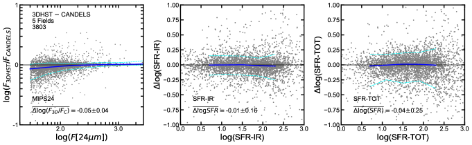
Figure D1.— Comparison of MIPS 24 $\mu$m fluxes and SFRs between the CANDELS (this work) and 3D-HST catalogs (Momcheva et al. 2016) in the 5 fields of the CANDELS survey. From left-to-right, comparison of the MIPS24 fluxes, IR-based SFRs and total (UV+IR) SFRs. The y-axis shows differences in 3D-HST minus CANDELS values. The comparison is restricted to galaxies detected above SNR$=$5 in MIPS24 in both catalogs. The blue lines show the running median and $\pm$1$\sigma$ scatter of the distribution whose average values are indicated in the bottom-left corner. The values in each panel have been corrected by a constant offset derived from the average running median. Overall, we find a good agreement in the fluxes and SFRs between the two catalogs. The CANDELS MIPS24 fluxes are only marginally brighter than the 3D-HST by $0.05$ dex. Such difference has little impact on the two SFRs which exhibit offsets of 0.01 and 0.04 dex, respectively.

Figure D1 shows the comparison of the MIPS 24 $\mu$m fluxes and SFRs (IR and total) between the CANDELS and 3D-HST catalogs. The blue and cyan lines indicate the running median and 1$\sigma$ percentiles. The values in each panel have been normalized by applying a constant offset (indicated in the bottom-left corner) determined from the average value of the running median. Overall, the comparison suggests that the values in the CANDELS and 3D-HST catalogs are quite consistent. The CANDELS MIPS24 fluxes are slightly brighter than the 3D-HST by 0.05 dex. This small difference is the same in the 5 cosmological fields, which suggest that the origin could be a small systematic difference in the photometric zero-points or perhaps in the value of the aperture correction. Interestingly, despite the small offset in the MIPS24 photometry, the IR-based SFRs are in excellent agreement with a median difference of just $\Delta$SFR$=-0.01$ dex. The $\sim$0.12 dex scatter in the comparison of IR-SFRs is also quite small compared for example to the 0.3 dex scatter in the comparison of stellar masses shown in § 5.3. Such small scatter is probably caused by small differences in the MIPS flux, redshift or the dust emission templates. Likewise, the comparison of total (UV+IR) SFRs shows an excellent agreement with an average offset of $\Delta$SFR$=-0.03$ dex and a slightly larger scatter of 0.21 dex. The increased scatter relative to the IR-SFRs comparison is likely caused by additional random differences in the UV-SFRs which are based on the different optical-to-NIR SED fitting of each work.

The L18 catalog aims to provide self-consistent far-IR to sub-mm photometry for galaxies in the GOODS-N region. As such, it is primarily selected in the far-IR, with the majority of the sources detected in a merged MIPS 24 + VLA 20cm catalog. Most of these sources have NIR counterparts, primarily in IRAC and K-band, which are used to crossmatch to other optical/NIR catalogs, such as the 3D-HST, for the purpose of obtaining optical-to-NIR photometry and photometric redshifts for each far-IR source. To first order, the L18 IR photometric measurements are similar to ours. They are both based on PSF fitting point-like sources using positional priors from other bands with higher spatial resolution. As appendix D.1, these priors help reduce the confusion effects due to crowding. The primary difference between the L18 and CANDELS methods is the choice of the detection priors. For any given band, we chose priors from the previous, shorter wavelength band with better resolution (e.g., MIPS24 priors for PACS100), while L18 use the full SEDs at shorter wavelengths to predict the fluxes of all the possible counterparts and, based on those, choose only the priors that are likely to be detected.

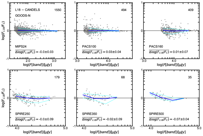
Figure D2.— Comparison of mid-to-far IR fluxes between the CANDELS (this work) and the Liu et al. (2018) catalogs in the GOODS-N field. From left-to-right and top-to-bottom, the panels show the comparison of the MIPS24, PACS100, PACS160, SPIRE250, SPIRE350 and SPIRE500 fluxes. The y-axis shows differences in L18 minus CANDELS values. The comparison is restricted to galaxies detected above SNR$=$5 in each band in both catalogs (see Table D1). The blue lines show the running median and $\pm$1$\sigma$ scatter of the distribution whose average values are indicated in the bottom-left corner. The values in each panel have been corrected by a constant offset derived from the average running median. The declining sensitivity and spatial resolution with increasing wavelength of the bands leads to fewer detections, larger scatter and some outliers likely caused by differences in the deblending of particularly crowded sources. Nonetheless, we find an overall good agreement in all bands with systematic offsets smaller than $\sim 0.1$ dex and a scatter that is roughly consistent with photometric uncertainties.

This “informed” choice of priors can ease the confusion around particularly crowded sources or can help find sources with peculiar SEDs (e.g., those detected in SPIRE but not in PACS). Nonetheless, as discussed in appendix D.1, the multiplicity in our sequential crossmatching method is very small (1:1 for MIPS and PACS and 3 or 2:1 for SPIRE) compared to that of a direct match from F160W or IRAC to SPIRE, where the multiplicity can be as high as 20 or 30. Thus, we expect that the bulk of the detections and IR fluxes in both catalogs to be in good agreement. The L18 catalog contains $\sim$3300 sources over a sligthly larger area of GOODS-N than that covered in the CANDELS survey. We crossmatch both catalogs within a 0$\farcs$5 radius and we sucessfully identify all the L18 sources that already had 3D-HST priors.

Figure D2 shows the photometric comparison between the six mid-to-far IR bands in common between the two catalogs. Each panel shows only galaxies detected at SNR$>5$ in both catalogs (see Table D1). As in Figure D1, the values have been corrected by a constant average offset determined from the running median (blue line). Overall, the photometry in the two catalogs exhibits a good agreement with only small systematic offsets ($\lesssim$0.03 dex in all bands but SPIRE500) and a typical scatter roughly consistent with the expected photometric uncertainties. Owing to its higher sensitivity and spatial resolution, the comparisons in the MIPS and PACS bands span a broader dynamical range ($\sim$1-1.5 dex) and include more galaxies, which leads a more homogeneous and smoother distribution. In SPIRE, however, both the dynamical range and the number of detections are smaller. Nonetheless, the bulk of the galaxies exhibit a good agreement with a scatter smaller than 0.1 dex.

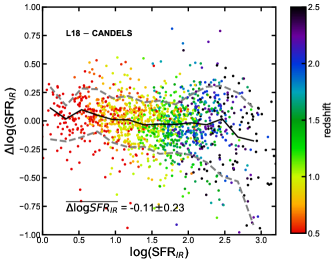
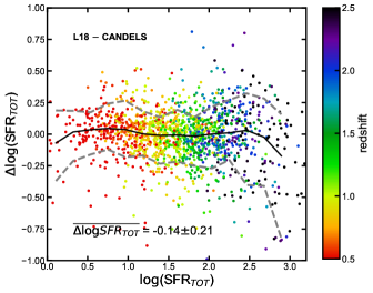
Figure D3.— Comparison of the IR-based SFRs (left) and total UV+IR SFRs (right) in the CANDELS (this work) and the Liu et al. (2018) catalogs in the GOODS-N field, color coded by redshift. The y-axis shows differences in L18 minus CANDELS values. The comparison is restricted to galaxies detected above SNR$=$5 in MIPS24 (the deepest band) in both catalogs. The black and grey lines show the running median and $\pm$1$\sigma$ scatter of the distribution whose average values are indicated in the bottom-left corner. The values in each panel have been corrected by a constant offset derived from the average running median. The CANDELS IR- and total- SFRs are only marginally larger than those in L18 by approximately constant values of 0.1 and 0.14 dex. There is no evidence for significant trends with SFR or redshift which appear somtimes due to strong features in the dust emission templated used in the IR-SED modeling. The scatter in the comparisons, $\lesssim 0.25$ dex, is consistent or even better than the typical 0.3 dex. Thus, we conclude that, overall, there is a good agreement betwee the CANDELS and L18 SFRs.

In addition to the far-IR photometry, we also compare the IR-based SFRs derived from the fitting of the full IR SEDs. This comparison depends on additional factors such as the number photometric fluxes in the IR SED, or the set of dust emission templates used for the fitting. The IR SEDs in L18 include a few more bands in the sub-mm and radio. However, those detections are restricted to only a few IR bright objects. Thus, the bulk of the sample has a similar SEDs in both catalogs. As for the fitting templates, L18 uses the Magdis et al. (2012) library plus 2 additional AGN models, while we use a combination of 3 libraries (see appendix D.2). Despite these differences, Figure D3 shows an excellent agreement in the SFRs with only a small average offset of $-0.1$ dex and a scatter of 0.21 dex, which is consistent with the typical uncertainties in these modeling-dependent comparisons. Furthermore, there is no evidence for any strong systematic offset with redshift. This is relevant because some dust emission templates exhibit strong spectral features, such as the PAH emission, that could bias the fit of some bands at specific redshifts. Lastly, the right panel of Figure D3 shows the comparison of the total (UV+IR) SFRs. We find again a good agreement with a similar average offset and scatter. This suggests that the impact of the UV-SFRs in the total SFRs of these IR bright galaxies is only minor and therefore small fluctuations in their values have a negligible impact in the comparison.

D.4. SFR catalogs and far-IR photometric flags

Table D5Description of the SFR catalog

Column No. Column Title Description 1 id Object identifier 2 z Photometric redshift used in the IR SED fitting, corresponds to zbest in the redshift catalog $3-16$ Flux, Flux_Err Flux and flux error in each filter. Filters are included in order: MIPS 24 and 70 $\mu$m, PACS 100 and 160$\mu$m and SPIRE 250, 350 and 500 $\mu$m [$\mu$Jy]. Galaxies without IR detections have upper limits in MIPS24 with Flux = 20 - 70 [$\mu$Jy] (see Table D1) and Flux_Err = 0. Upper limits in MIPS24 are used to estimate upper limits in SFR-IR, indicated with negative values. 17 SFR${}_{\rm total}^{\rm ladder}$ Use as default SFR. Best estimate of the total SFR: either SFR_IR+SFR${}_{\rm UV}^{\rm obs}$ for IR detected sources or SFR${}_{\rm UV}^{\rm corr}$ for the rest. 18 SFR_ladder_type Type of SFR indicators used in SFR${}_{\rm total}^{\rm ladder}$: 1 for SFR${}_{\rm total}^{\rm ladder}$ = SFR${}_{\rm IR}^{\rm fit}$ + SFR${}_{\rm UV}^{\rm obs}$ 2 for SFR${}_{\rm total}^{\rm ladder}$ = SFR${}_{\rm IR}^{\rm W11}$ + SFR${}_{\rm UV}^{\rm obs}$ 3 for SFR${}_{\rm total}^{\rm ladder}$ = SFR${}_{\rm UV}^{\rm corr}$ 19 SFR${}_{\rm UV}^{\rm corr}$ UV-based star formation rate corrected for extinction using the IRX-$\beta_{\rm UV}$ relations. This value is a weighted average of SFR${}_{\rm UV}^{\rm corr}$(160) and SFR${}_{\rm UV}^{\rm corr}$(280) 20 SFR${}_{\rm UV}^{\rm corr}$_Err Uncertainty in the UV-based star formation rate corrected for extinction. 21 SFR_IR IR-based star formation rate. This value is equal to: SFR_IR = SFR${}_{\rm IR}^{\rm fit}$ when SFR_ladder_type=1. SFR_IR = SFR${}_{\rm IR}^{\rm W11}$ when SFR_ladder_type=2. SFR_IR = -SFR${}_{\rm IR}^{\rm W11}$ when SFR_ladder_type=3 (based on upper limits in MIPS24). 22 SFR${}_{\rm UV}^{\rm obs}(160)$ UV-based star formation rate not corrected for extinction determined from the UV luminosity at 160 nm. 23 SFR${}_{\rm UV}^{\rm obs}(280)$ UV-based star formation rate not corrected for extinction determined from the UV luminosity at 280 nm.. 24 $\beta_{\rm UV}$ UV slope 25 $A_{\rm UV}(160)$ UV attenuation derived from the IRX-$\beta_{\rm UV}$ calibration for SFR${}_{\rm UV}^{\rm obs}$(160) 26 $A_{\rm UV}(280)$ UV attenuation derived from the IRX-$\beta_{\rm UV}$ calibration for SFR${}_{\rm UV}^{\rm obs}$(280) 27 $A$(V) Optical attenuation in the V-band derived from $A_{\rm UV}$ by assuming a Calzetti et al. (2000) attenuation law. 28 SFR${}_{\rm IR}^{\rm W11}$ IR-based star formation rate derived from the MIPS 24$\mu$m flux following (Wuyts et al. 2011b). 29 SFR${}_{\rm UV}^{\rm corr}(160)$ UV-based star formation rate corrected for extinction using the IRX-$\beta_{\rm UV}$ relations determined from the UV luminosity at 160 nm. 30 SFR${}_{\rm UV}^{\rm corr}(280)$ UV-based star formation rate corrected for extinction using the IRX-$\beta_{\rm UV}$ relations determined from the UV luminosity at 280 nm.

Table D6Description of the SFR Flag catalogs

Column No. Column Title Description 1 id Object identifier in the F160W catalog 2 MIPS_ID_order ID of the MIPS24 counterpart in the catalog from Pérez-Gonález et al. (2018) Multiple F160W counterparts can be associated with this source the order of likelihood is indicated with _1,_2, etc. 3 MIPS_discriminator Criteria used to determine the likelihood order of the F160W counterparts to a MIPS source: mips24, irac3.6, irac8.0, dist There is only one counterpart within 2$\farcs$5 (mips24), or the primary counterpart in the brightest this IRAC band or it is the closest in coordinates (dist) 4–9 Flux, Flux_Err Flux and flux error in the MIPS24, IRAC80, IRAC36 filters. In units of $\mu$Jy. 10 MIPS_distance Distance between the F160W source and the closest MIPS source in arcsec. 11 MIPS_order Likelihood of being the F160W source being true counterpart of the MIPS source. From 1 to N, with 1 being the highest. 12 MIPS_n_counterparts Number of F160W counterparts candidates for the closest MIPS source within 2$\farcs$5. 13 MIPS24_snr_cuts Flag regarding the SNR cuts applied in MIPS24: 0 no-flux, 1 flux $>$ SNR limit, -1 flux $<$ SNR limit. Only sources with flag ¿ 0 are included in table D5. 14–18 N_F160W_MIPS24_PSF Number of F160W counterparts within 1, 0.5, 0.25, 2, 3 times the size of the MIPS24 PSF (2$\farcs$0) around the MIPS24 primary. 19–23 N_F160W_MIPS24_WCS Number of F160W counterparts within 1, 0.5, 0.25, 2, 3 times the size of the WCS accuracy of the MIPS24 mosaic (2$\farcs$0)around the MIPS24 primary. 24–28 N_MIPS24_MIPS24_PSF Number of MIPS24 counterparts within 1, 0.5, 0.25, 2, 3 times the size of the MIPS24 PSF (2$\farcs$0) around the MIPS24 primary. 29–33 N_MIPS24_MIPS24_WCS Number of MIPS24 counterparts within 1, 0.5, 0.25, 2, 3 times the size of the WCS accuracy of the MIPS24 mosaic (2$\farcs$0) around the MIPS24 primary. 34–38 N_IRAC36_MIPS24_PSF Number of IRAC36 counterparts within 1, 0.5, 0.25, 2, 3 times the size of the MIPS24 PSF (2$\farcs$0) around the MIPS24 primary. 39–43 N_IRAC36_MIPS24_WCS Number of IRAC36 counterparts within 1, 0.5, 0.25, 2, 3 times the size of the WCS accuracy of the MIPS24 mosaic (2$\farcs$0) around the MIPS24 primary. 1 id Object identifier in the F160W catalog 2 PACS_ID_order ID of the PACS counterpart in the catalog from Pérez-Gonález et al. (2008,2010) Multiple F160W counterparts can be associated with this source the order of likelihood is indicated with _1,_2, etc. 3 PACS_discriminator Criteria used to determine the likelihood order of the F160W counterparts to a PACS source: pacs160, pacs100, mips24, irac3.6, irac8.0, dist There is only one counterpart within 3$\farcs$0 (pacs160/pac100), or the primary counterpart in the brightest this MIPS/IRAC band or it is the closest in coordinates (dist) 4–13 Flux, Flux_Err Flux and flux error in the PACS160, PACS100, MIPS24, IRAC80, IRAC36 filters. In units of $\mu$Jy. 14 PACS_distance Distance between the F160W source and the closest PACS source within 3$\farcs$0. 15 PACS_order Likelihood of being the F160W source being true counterpart of the PACS source. From 1 to N, with 1 being the highest. 16 PACS_n_counterparts Number of F160W counterparts candidates for the closest PACS source (IN WHICH RADIUS). 17 PACS100_snr_cuts Flag regarding the SNR cuts applied in PACS100: 0 no-flux, 1 flux $>$ SNR limit, -1 flux $<$ SNR limit. Only sources with flag ¿ 0 are included in table D5. 18 PACS160_snr_cuts Flag regarding the SNR cuts applied in PACS160: 0 no-flux, 1 flux $>$ SNR limit, -1 flux $<$ SNR limit. Only sources with flag ¿ 0 are included in table D5. 19–28 N_F160W_PACS_PSF Number of F160W counterparts within 1, 0.5, 0.25, 2, 3 times the size of the PACS100 and PACS160 PSF (4$\farcs$5/7$\farcs$0) around the PACS primary. 29–38 N_F160W_PACS_WCS Number of F160W counterparts within 1, 0.5, 0.25, 2, 3 times the size of the WCS accuracy of the PACS100 and PACS160 mosaics (2$\farcs$0/2$\farcs$5) around the PACS primary. 39–48 N_PACS_PACS_PSF Number of PACS counterparts within 1, 0.5, 0.25, 2, 3 times the size of the PACS100 and PACS160 PSF (4$\farcs$5/7$\farcs$0) around the PACS primary. 49–58 N_PACS_PACS_WCS Number of PACS counterparts within 1, 0.5, 0.25, 2, 3 times the size of the WCS accuracy of the PACS100 and PACS160 mosaics (2$\farcs$0/2$\farcs$5) around the PACS primary. 59–68 N_MIPS24_PACS_PSF Number of MIPS24 counterparts within 1, 0.5, 0.25, 2, 3 times the size of the PACS100 and PACS160 PSF (4$\farcs$5/7$\farcs$0) around the PACS primary. 69–78 N_MIPS24_PACS_WCS Number of MIPS24 counterparts within 1, 0.5, 0.25, 2, 3 times the size of the WCS accuracy of the PACS100 and PACS160 mosaics (2$\farcs$0/2$\farcs$5) around the PACS primary. 79–88 N_IRAC36_PACS_PSF Number of IRAC36 counterparts within 1, 0.5, 0.25, 2, 3 times the size of the PACS100 and PACS160 PSF (4$\farcs$5/7$\farcs$0) around the PACS primary. 89–98 N_IRAC36_PACS_WCS Number of IRAC36 counterparts within 1, 0.5, 0.25, 2, 3 times the size of the WCS accuracy of the PACS100 and PACS160 mosaics (2$\farcs$0/2$\farcs$5) around the PACS primary. 1 id Object identifier in the F160W catalog 2 SPIRE_ID_order ID of the SPIRE counterpart in the catalog from Pérez-Gonález et al. (2008,2010) Multiple F160W counterparts can be associated with this source the order of likelihood is indicated with _1,_2, etc. 3 SPIRE_discriminator Criteria used to determine the likelihood order of the F160W counterparts to a SPIRE source: spire500, spire350, spire250, pacs160, pacs100, mips24, irac3.6, irac8.0, dist There is only one counterpart within 9$\farcs$0 (spire500,350,250), or the primary counterpart in the brightest this PACS/MIPS/IRAC band or it is the closest in coordinates (dist) 4–19 Flux, Flux_Err Flux and flux error in the PACS160, PACS100, MIPS24, IRAC80, IRAC36 filters. In units of $\mu$Jy. 20 SPIRE_distance Distance between the F160W source and the closest SPIRE source in arcsec. 21 SPIRE_order Likelihood of being the F160W source being true counterpart of the SPIRE source. From 1 to N, with 1 being the highest. 22 SPIRE_n_counterparts Number of F160W counterparts candidates for the closest SPIRE source within 9$\farcs$0. 23 SPIRE250_snr_cuts Flag regarding the SNR cuts applied in SPIRE250: 0 no-flux, 1 flux $>$ SNR limit, -1 flux $<$ SNR limit. Only sources with flag ¿ 0 are included in table D5. 24 SPIRE350_snr_cuts Flag regarding the SNR cuts applied in SPIRE350: 0 no-flux, 1 flux $>$ SNR limit, -1 flux $<$ SNR limit. Only sources with flag ¿ 0 are included in table D5. 25 SPIRE500_snr_cuts Flag regarding the SNR cuts applied in SPIRE500: 0 no-flux, 1 flux $>$ SNR limit, -1 flux $<$ SNR limit. Only sources with flag ¿ 0 are included in table D5. 26–30 N_F160W_SPIRE_PSF Number of F160W counterparts within 1, 0.5, 0.25, 2, 3 times the size of the SPIRE250, SPIRE 350 and SPIRE500 PSF (11$\farcs$0/11$\farcs$0/17$\farcs$0) around the SPIRE primary. 41–55 N_F160W_SPIRE_WCS Number of F160W counterparts within 1, 0.5, 0.25, 2, 3 times the size of the WCS accuracy of the SPIRE250, SPIRE 350 and SPIRE500 mosaics (9$\farcs$0/9$\farcs$0/15$\farcs$0) around the SPIRE primary. 56–70 N_SPIRE_SPIRE_PSF Number of SPIRE counterparts within 1, 0.5, 0.25, 2, 3 times the size of the SPIRE250, SPIRE 350 and SPIRE500 PSF (11$\farcs$0/11$\farcs$0/17$\farcs$0) around the SPIRE primary. 71–85 N_SPIRE_SPIRE_WCS Number of SPIRE counterparts within 1, 0.5, 0.25, 2, 3 times the size of the WCS accuracy of the SPIRE250, SPIRE 350 and SPIRE500 mosaics (9$\farcs$0/9$\farcs$0/15$\farcs$0) around the SPIRE primary. 86–100 N_PACS_SPIRE_PSF Number of PACS counterparts within 1, 0.5, 0.25, 2, 3 times the size of the SPIRE250, SPIRE 350 and SPIRE500 PSF (11$\farcs$0/11$\farcs$0/17$\farcs$0) around the SPIRE primary. 101–115 N_PACS_SPIRE_WCS Number of PACS counterparts within 1, 0.5, 0.25, 2, 3 times the size of the WCS accuracy of the SPIRE250, SPIRE 350 and SPIRE500 mosaics (9$\farcs$0/9$\farcs$0/15$\farcs$0) around the SPIRE primary. 116–130 N_MIPS_SPIRE_PSF Number of MIPS counterparts within 1, 0.5, 0.25, 2, 3 times the size of the SPIRE250, SPIRE 350 and SPIRE500 PSF (11$\farcs$0/11$\farcs$0/17$\farcs$0) around the SPIRE primary. 131–145 N_MIPS_SPIRE_WCS Number of MIPS counterparts within 1, 0.5, 0.25, 2, 3 times the size of the WCS accuracy of the SPIRE250, SPIRE 350 and SPIRE500 mosaics (9$\farcs$0/9$\farcs$0/15$\farcs$0) around the SPIRE primary. 146–160 N_IRAC36_SPIRE_PSF Number of IRAC36 counterparts within 1, 0.5, 0.25, 2, 3 times the size of the SPIRE250, SPIRE 350 and SPIRE500 PSF (11$\farcs$0/11$\farcs$0/17$\farcs$0) around the SPIRE primary. 161–175 N_IRAC36_SPIRE_WCS Number of IRAC36 counterparts within 1, 0.5, 0.25, 2, 3 times the size of the WCS accuracy of the SPIRE250, SPIRE 350 and SPIRE500 mosaics (9$\farcs$0/9$\farcs$0/15$\farcs$0) around the SPIRE primary.

This section describes the content of the FIR photometry and SFR catalogs for all sources in the 5 CANDELS fields. Table D5 contains the FIR fluxes, dust attenuations and different SFR tracers computed following the methods described in § 5.4 and appendix D.1 . In addition Table D6, provides FIR photometric and proximity flags that can be used to clean the catalog or to apply more restrictive conditions on the sources with FIR detections.

Note that, while in Table D5 there is only one possible F160W counterpart to each detection in a FIR band, the catalog described in Table D6 list all the possible F160W counterparts to a given FIR source (MIPS, PACS and SPIRE) indicating their likelihood (from 1 to N) of being the primary counterpart of the IR detection. Only the F160W sources with the maximum likelihood (e.g., MIPS_order=1) have IR fluxes in Table D5. The total number of F160W counterparts to a given IR source as well as their distances such source and their respective IRAC fluxes are also indicated.

In addition to the F160W multiplicity for a given FIR source, the catalog lists the multiplicity of that source in all other mid-to-far IR bands up to itself. These multiplicities are computed for several cross-match radius relative to the typical spatial resolution of the FIR band (e.g., radius of 0.5, 1, 2 or 3$\times$ the FWHM of the PSF). For the example, the MIPS flag catalog includes the multiplicities of F160W, IRAC and MIPS sources within different radius. The PACS flag catalog includes multiplicities of F160W, IRAC, MIPS and PACS sources, etc. The values in the flag catalogs provide a quick a simple way to find relative isolated FIR sources, or to identify FIR sources in crowded environments which might lead to some contamination in the photometry.

References

- Acquaviva et al. (2011) Acquaviva, V., Gawiser, E., & Guaita, L. 2011, ApJ, 737, 47
- Alexander et al. (2003) Alexander, D. M., Bauer, F. E., Brandt, W. N., et al. 2003, AJ, 126, 539
- Arnouts & Ilbert (2011) Arnouts, S., & Ilbert, O. 2011, LePHARE: Photometric Analysis for Redshift Estimate, Astrophysics Source Code Library
- Ashby et al. (2015) Ashby, M. L. N., Willner, S. P., Fazio, G. G., et al. 2015, ApJS, 218, 33
- Ashby et al. (2013) —. 2013, ApJ, 769, 80
- Atek et al. (2010) Atek, H., Malkan, M., McCarthy, P., et al. 2010, ApJ, 723, 104
- Barden et al. (2012) Barden, M., Häußler, B., Peng, C. Y., et al. 2012, MNRAS, 422, 449
- Barger et al. (2008) Barger, A. J., Cowie, L. L., & Wang, W.-H. 2008, ApJ, 689, 687
- Barro et al. (2014) Barro, G., Faber, S. M., Pérez-González, P. G., et al. 2014, ApJ, 791, 52
- Barro et al. (2011) Barro, G., Pérez-González, P. G., Gallego, J., et al. 2011, ApJS, 193, 30
- Bell et al. (2003) Bell, E. F., McIntosh, D. H., Katz, N., et al. 2003, ApJS, 149, 289
- Bell et al. (2005) Bell, E. F., Papovich, C., Wolf, C., et al. 2005, ApJ, 625, 23
- Bell et al. (2012) Bell, E. F., van der Wel, A., Papovich, C., et al. 2012, ApJ, 753, 167
- Berta et al. (2011) Berta, S., Magnelli, B., Nordon, R., et al. 2011, A&A, 532, A49
- Bertin (2010) Bertin, E. 2010, SWarp: Resampling and Co-adding FITS Images Together, Astrophysics Source Code Library
- Bertin & Arnouts (1996) Bertin, E., & Arnouts, S. 1996, A&AS, 117, 393
- Bezanson et al. (2016) Bezanson, R., Wake, D. A., Brammer, G. B., et al. 2016, ApJ, 822, 30
- Bolzonella et al. (2000) Bolzonella, M., Miralles, J.-M., & Pelló, R. 2000, A&A, 363, 476
- Bouwens et al. (2016) Bouwens, R. J., Oesch, P. A., Labbé, I., et al. 2016, ApJ, 830, 67
- Brammer et al. (2014) Brammer, G., Kelly, P., Rodney, S., et al. 2014, The Astronomer’s Telegram, 5728
- Brammer et al. (2015) Brammer, G., Ryan, R., & Pirzkal, N. 2015, Source-dependent master sky images for the WFC3/IR grisms, Tech. rep.
- Brammer et al. (2008) Brammer, G. B., van Dokkum, P. G., & Coppi, P. 2008, ApJ, 686, 1503
- Brammer et al. (2012) Brammer, G. B., van Dokkum, P. G., Franx, M., et al. 2012, ApJS, 200, 13
- Brammer et al. (2011) Brammer, G. B., Whitaker, K. E., van Dokkum, P. G., et al. 2011, ApJ, 739, 24
- Bruzual & Charlot (2003) Bruzual, G., & Charlot, S. 2003, MNRAS, 344, 1000
- Buat et al. (2005) Buat, V., Iglesias-Páramo, J., Seibert, M., et al. 2005, ApJ, 619, L51
- Buat et al. (2012) Buat, V., Noll, S., Burgarella, D., et al. 2012, A&A, 545, A141
- Buat et al. (2007) Buat, V., Takeuchi, T. T., Iglesias-Páramo, J., et al. 2007, ApJS, 173, 404
- Calzetti et al. (2000) Calzetti, D., Armus, L., Bohlin, R. C., et al. 2000, ApJ, 533, 682
- Capak et al. (2004) Capak, P., Cowie, L. L., Hu, E. M., et al. 2004, AJ, 127, 180
- Casey et al. (2014) Casey, C. M., Scoville, N. Z., Sanders, D. B., et al. 2014, ApJ, 796, 95
- Cava et al. (2015) Cava, A., Pérez-González, P. G., Eliche-Moral, M. C., et al. 2015, ApJ, 812, 155
- Chabrier (2003) Chabrier, G. 2003, PASP, 115, 763
- Chapman et al. (2005) Chapman, S. C., Blain, A. W., Smail, I., et al. 2005, ApJ, 622, 772
- Charlot & Fall (2000) Charlot, S., & Fall, S. M. 2000, ApJ, 539, 718
- Chary & Elbaz (2001) Chary, R., & Elbaz, D. 2001, ApJ, 556, 562
- Cooper et al. (2011) Cooper, M. C., Aird, J. A., Coil, A. L., et al. 2011, ApJS, 193, 14
- Cowie et al. (2004) Cowie, L. L., Barger, A. J., Hu, E. M., et al. 2004, AJ, 127, 3137
- Daddi et al. (2004) Daddi, E., Cimatti, A., Renzini, A., et al. 2004, ApJ, 617, 746
- Daddi et al. (2007) Daddi, E., Dickinson, M., Morrison, G., et al. 2007, ApJ, 670, 156
- Daddi et al. (2005) Daddi, E., Renzini, A., Pirzkal, N., et al. 2005, ApJ, 626, 680
- Dahlen et al. (2013) Dahlen, T., Mobasher, B., Faber, S. M., et al. 2013, ApJ, 775, 93
- Dale et al. (2009) Dale, D. A., Cohen, S. A., Johnson, L. C., et al. 2009, ApJ, 703, 517
- Dale & Helou (2002) Dale, D. A., & Helou, G. 2002, ApJ, 576, 159
- Dickinson et al. (2003) Dickinson, M., Bergeron, J., Casertano, S., et al. 2003, Great Observatories Origins Deep Survey (GOODS) Validation Observations, Spitzer Proposal
- Draine & Li (2007) Draine, B. T., & Li, A. 2007, ApJ, 657, 810
- Duncan et al. (2014) Duncan, K., Conselice, C. J., Mortlock, A., et al. 2014, MNRAS, 444, 2960
- Elbaz et al. (2011) Elbaz, D., Dickinson, M., Hwang, H. S., et al. 2011, A&A, 533, A119
- Erb et al. (2010) Erb, D. K., Pettini, M., Shapley, A. E., et al. 2010, ApJ, 719, 1168
- Fazio et al. (2004) Fazio, G. G., Ashby, M. L. N., Barmby, P., et al. 2004, ApJS, 154, 39
- Ferreras et al. (2009) Ferreras, I., Pasquali, A., Malhotra, S., et al. 2009, ApJ, 706, 158
- Finkelstein et al. (2015) Finkelstein, S. L., Ryan, Jr., R. E., Papovich, C., et al. 2015, ApJ, 810, 71
- Fontana et al. (2000) Fontana, A., D’Odorico, S., Poli, F., et al. 2000, AJ, 120, 2206
- Foreman-Mackey et al. (2013) Foreman-Mackey, D., Hogg, D. W., Lang, D., et al. 2013, PASP, 125, 306
- Franx et al. (2008) Franx, M., van Dokkum, P. G., Schreiber, N. M. F., et al. 2008, ApJ, 688, 770
- Frayer et al. (2006) Frayer, D. T., Huynh, M. T., Chary, R., et al. 2006, ApJ, 647, L9
- Galametz et al. (2013) Galametz, A., Grazian, A., Fontana, A., et al. 2013, ApJS, 206, 10
- Giallongo et al. (2008) Giallongo, E., Ragazzoni, R., Grazian, A., et al. 2008, A&A, 482, 349
- Giavalisco et al. (2004) Giavalisco, M., Ferguson, H. C., Koekemoer, A. M., et al. 2004, ApJ, 600, L93
- Gonzaga & et al. (2012) Gonzaga, S., & et al. 2012, The DrizzlePac Handbook
- Grazian et al. (2015) Grazian, A., Fontana, A., Santini, P., et al. 2015, A&A, 575, A96
- Grazian et al. (2017) Grazian, A., Giallongo, E., Paris, D., et al. 2017, A&A, 602, A18
- Griffin et al. (2010) Griffin, M. J., Abergel, A., Abreu, A., et al. 2010, A&A, 518, L3
- Grogin et al. (2011) Grogin, N. A., Kocevski, D. D., Faber, S. M., et al. 2011, ApJS, 197, 35
- Gunn & Stryker (1983) Gunn, J. E., & Stryker, L. L. 1983, ApJS, 52, 121
- Guo et al. (2015) Guo, Y., Ferguson, H. C., Bell, E. F., et al. 2015, ApJ, 800, 39
- Guo et al. (2013) Guo, Y., Ferguson, H. C., Giavalisco, M., et al. 2013, ApJS, 207, 24
- Heckman et al. (1998) Heckman, T. M., Robert, C., Leitherer, C., et al. 1998, ApJ, 503, 646
- Hsu et al. (2019) Hsu, L.-T., Lin, L., Dickinson, M., et al. 2019, ApJ, 871, 233
- Huertas-Company et al. (2015) Huertas-Company, M., Gravet, R., Cabrera-Vives, G., et al. 2015, ApJS, 221, 8
- Ilbert et al. (2009) Ilbert, O., Capak, P., Salvato, M., et al. 2009, ApJ, 690, 1236
- Ilbert et al. (2010) Ilbert, O., Salvato, M., Le Floc’h, E., et al. 2010, ApJ, 709, 644
- Kajisawa et al. (2009) Kajisawa, M., Ichikawa, T., Tanaka, I., et al. 2009, ApJ, 702, 1393
- Kajisawa et al. (2011) —. 2011, PASJ, 63, 379
- Kartaltepe et al. (2010) Kartaltepe, J. S., Sanders, D. B., Le Floc’h, E., et al. 2010, ApJ, 709, 572
- Kennicutt (1998) Kennicutt, Jr., R. C. 1998, ARA&A, 36, 189
- Koekemoer et al. (2011) Koekemoer, A. M., Faber, S. M., Ferguson, H. C., et al. 2011, ApJS, 197, 36
- Kong et al. (2004) Kong, X., Charlot, S., Brinchmann, J., et al. 2004, MNRAS, 349, 769
- Kriek et al. (2015) Kriek, M., Shapley, A. E., Reddy, N. A., et al. 2015, ApJS, 218, 15
- Kriek et al. (2009) Kriek, M., van Dokkum, P. G., Franx, M., et al. 2009, ApJ, 705, L71
- Krist (1995) Krist, J. 1995, in Astronomical Society of the Pacific Conference Series, Vol. 77, Astronomical Data Analysis Software and Systems IV, ed. R. A. Shaw, H. E. Payne, & J. J. E. Hayes, 349
- Kron (1980) Kron, R. G. 1980, ApJS, 43, 305
- Labbé et al. (2006) Labbé, I., Bouwens, R., Illingworth, G. D., et al. 2006, ApJ, 649, L67
- Labbé et al. (2005) Labbé, I., Huang, J., Franx, M., et al. 2005, ApJ, 624, L81
- Labbé et al. (2013) Labbé, I., Oesch, P. A., Bouwens, R. J., et al. 2013, ApJ, 777, L19
- Laidler et al. (2007) Laidler, V. G., Papovich, C., Grogin, N. A., et al. 2007, PASP, 119, 1325
- Lee et al. (2012) Lee, K.-S., Ferguson, H. C., Wiklind, T., et al. 2012, ApJ, 752, 66
- Leitherer et al. (2014) Leitherer, C., Ekström, S., Meynet, G., et al. 2014, ApJS, 212, 14
- Liu et al. (2018) Liu, D., Daddi, E., Dickinson, M., et al. 2018, ApJ, 853, 172
- Lutz et al. (2011) Lutz, D., Poglitsch, A., Altieri, B., et al. 2011, A&A, 532, A90
- Magdis et al. (2012) Magdis, G. E., Daddi, E., Béthermin, M., et al. 2012, ApJ, 760, 6
- Magnelli et al. (2009) Magnelli, B., Elbaz, D., Chary, R. R., et al. 2009, A&A, 496, 57
- Magnelli et al. (2013) Magnelli, B., Popesso, P., Berta, S., et al. 2013, A&A, 553, A132
- Marchesini et al. (2009) Marchesini, D., van Dokkum, P. G., Förster Schreiber, N. M., et al. 2009, ApJ, 701, 1765
- McLure et al. (2018) McLure, R. J., Dunlop, J. S., Cullen, F., et al. 2018, MNRAS, 476, 3991
- Merlin et al. (2016) Merlin, E., Bourne, N., Castellano, M., et al. 2016, A&A, 595, A97
- Merlin et al. (2015) Merlin, E., Fontana, A., Ferguson, H. C., et al. 2015, A&A, 582, A15
- Meurer et al. (1999) Meurer, G. R., Heckman, T. M., & Calzetti, D. 1999, ApJ, 521, 64
- Meurer et al. (1997) Meurer, G. R., Heckman, T. M., Lehnert, M. D., et al. 1997, AJ, 114, 54
- Mobasher et al. (2015) Mobasher, B., Dahlen, T., Ferguson, H. C., et al. 2015, ApJ, 808, 101
- Momcheva et al. (2016) Momcheva, I. G., Brammer, G. B., van Dokkum, P. G., et al. 2016, ApJS, 225, 27
- Mortlock et al. (2015) Mortlock, A., Conselice, C. J., Hartley, W. G., et al. 2015, MNRAS, 447, 2
- Muzzin et al. (2013) Muzzin, A., Marchesini, D., Stefanon, M., et al. 2013, ApJ, 777, 18
- Narayanan et al. (2018) Narayanan, D., Conroy, C., Davé, R., et al. 2018, ApJ, 869, 70
- Nayyeri et al. (2017) Nayyeri, H., Hemmati, S., Mobasher, B., et al. 2017, ApJS, 228, 7
- Noeske et al. (2007) Noeske, K. G., Weiner, B. J., Faber, S. M., et al. 2007, ApJ, 660, L43
- Nordon et al. (2013) Nordon, R., Lutz, D., Saintonge, A., et al. 2013, ApJ, 762, 125
- Oke (1974) Oke, J. B. 1974, ApJS, 27, 21
- Oliver et al. (2012) Oliver, S. J., Bock, J., Altieri, B., et al. 2012, MNRAS, 424, 1614
- Overzier et al. (2010) Overzier, R. A., Heckman, T. M., Schiminovich, D., et al. 2010, ApJ, 710, 979
- Overzier et al. (2011) Overzier, R. A., Heckman, T. M., Wang, J., et al. 2011, ApJ, 726, L7
- Papovich et al. (2001) Papovich, C., Dickinson, M., & Ferguson, H. C. 2001, ApJ, 559, 620
- Papovich et al. (2015) Papovich, C., Labbé, I., Quadri, R., et al. 2015, ApJ, 803, 26
- Papovich et al. (2006) Papovich, C., Moustakas, L. A., Dickinson, M., et al. 2006, ApJ, 640, 92
- Papovich et al. (2007) Papovich, C., Rudnick, G., Le Floc’h, E., et al. 2007, ApJ, 668, 45
- Pérez-González et al. (2013) Pérez-González, P. G., Cava, A., Barro, G., et al. 2013, ApJ, 762, 46
- Pérez-González et al. (2010) Pérez-González, P. G., Egami, E., Rex, M., et al. 2010, A&A, 518, L15+
- Pérez-González et al. (2005) Pérez-González, P. G., Rieke, G. H., Egami, E., et al. 2005, ApJ, 630, 82
- Pérez-González et al. (2008) Pérez-González, P. G., Rieke, G. H., Villar, V., et al. 2008, ApJ, 675, 234
- Pettini et al. (1998) Pettini, M., Kellogg, M., Steidel, C. C., et al. 1998, ApJ, 508, 539
- Poglitsch et al. (2010) Poglitsch, A., Waelkens, C., Geis, N., et al. 2010, A&A, 518, L2
- Pope et al. (2008) Pope, A., Bussmann, R. S., Dey, A., et al. 2008, ApJ, 689, 127
- Popping et al. (2017) Popping, G., Decarli, R., Man, A. W. S., et al. 2017, ArXiv e-prints
- Rawle et al. (2016) Rawle, T. D., Altieri, B., Egami, E., et al. 2016, MNRAS
- Reddy et al. (2010) Reddy, N. A., Erb, D. K., Pettini, M., et al. 2010, ApJ, 712, 1070
- Reddy et al. (2018) Reddy, N. A., Shapley, A. E., Sanders, R. L., et al. 2018, ApJ, 869, 92
- Reddy et al. (2006) Reddy, N. A., Steidel, C. C., Erb, D. K., et al. 2006, ApJ, 653, 1004
- Reddy et al. (2008) Reddy, N. A., Steidel, C. C., Pettini, M., et al. 2008, ApJS, 175, 48
- Rieke et al. (2009) Rieke, G. H., Alonso-Herrero, A., Weiner, B. J., et al. 2009, ApJ, 692, 556
- Riess et al. (2007) Riess, A. G., Strolger, L.-G., Casertano, S., et al. 2007, ApJ, 659, 98
- Rodríguez-Muñoz et al. (2019) Rodríguez-Muñoz, L., Rodighiero, G., Mancini, C., et al. 2019, MNRAS, 485, 586
- Rothberg et al. (2016) Rothberg, B., Kuhn, O., Edwards, M. L., et al. 2016, in Proc. SPIE, Vol. 9906, Ground-based and Airborne Telescopes VI, 990622
- Rujopakarn et al. (2013) Rujopakarn, W., Rieke, G. H., Weiner, B. J., et al. 2013, ApJ, 767, 73
- Salmon et al. (2015) Salmon, B., Papovich, C., Finkelstein, S. L., et al. 2015, ApJ, 799, 183
- Santini et al. (2015) Santini, P., Ferguson, H. C., Fontana, A., et al. 2015, ApJ, 801, 97
- Schreiber et al. (2015a) Schreiber, C., Pannella, M., Elbaz, D., et al. 2015a, A&A, 575, A74
- Schreiber et al. (2015b) —. 2015b, A&A, 575, A74
- Scoville et al. (2016) Scoville, N., Sheth, K., Aussel, H., et al. 2016, ApJ, 820, 83
- Skelton et al. (2014) Skelton, R. E., Whitaker, K. E., Momcheva, I. G., et al. 2014, ApJS, 214, 24
- Skrutskie et al. (2006) Skrutskie, M. F., Cutri, R. M., Stiening, R., et al. 2006, AJ, 131, 1163
- Speagle et al. (2014) Speagle, J. S., Steinhardt, C. L., Capak, P. L., et al. 2014, ApJS, 214, 15
- Stefanon et al. (2017) Stefanon, M., Yan, H., Mobasher, B., et al. 2017, ArXiv e-prints
- Straatman et al. (2014) Straatman, C. M. S., Labbé, I., Spitler, L. R., et al. 2014, ApJ, 783, L14
- Straatman et al. (2016) Straatman, C. M. S., Spitler, L. R., Quadri, R. F., et al. 2016, ApJ, 830, 51
- Symeonidis et al. (2008) Symeonidis, M., Willner, S. P., Rigopoulou, D., et al. 2008, MNRAS, 385, 1015
- Tal et al. (2014) Tal, T., Dekel, A., Oesch, P., et al. 2014, ApJ, 789, 164
- Treu et al. (2015) Treu, T., Schmidt, K. B., Brammer, G. B., et al. 2015, ApJ, 812, 114
- Trump et al. (2013) Trump, J. R., Konidaris, N. P., Barro, G., et al. 2013, ApJ, 763, L6
- van der Wel et al. (2012) van der Wel, A., Bell, E. F., Häussler, B., et al. 2012, ApJS, 203, 24
- van der Wel et al. (2014) van der Wel, A., Franx, M., van Dokkum, P. G., et al. 2014, ApJ, 788, 28
- Wang et al. (2016) Wang, T., Elbaz, D., Schreiber, C., et al. 2016, ApJ, 816, 84
- Whitaker et al. (2014) Whitaker, K. E., Franx, M., Leja, J., et al. 2014, ApJ, 795, 104
- Whitaker et al. (2012) Whitaker, K. E., Kriek, M., van Dokkum, P. G., et al. 2012, ApJ, 745, 179
- Whitaker et al. (2011) Whitaker, K. E., Labbé, I., van Dokkum, P. G., et al. 2011, ApJ, 735, 86
- Wiklind et al. (2008) Wiklind, T., Dickinson, M., Ferguson, H. C., et al. 2008, ApJ, 676, 781
- Williams et al. (1996) Williams, R. E., Blacker, B., Dickinson, M., et al. 1996, AJ, 112, 1335
- Williams et al. (2009) Williams, R. J., Quadri, R. F., Franx, M., et al. 2009, ApJ, 691, 1879
- Wirth et al. (2015) Wirth, G. D., Trump, J. R., Barro, G., et al. 2015, AJ, 150, 153
- Wirth et al. (2004) Wirth, G. D., Willmer, C. N. A., Amico, P., et al. 2004, AJ, 127, 3121
- Witt & Gordon (2000) Witt, A. N., & Gordon, K. D. 2000, ApJ, 528, 799
- Wolf et al. (2001) Wolf, C., Dye, S., Kleinheinrich, M., et al. 2001, A&A, 377, 442
- Wolf et al. (2003) Wolf, C., Meisenheimer, K., Rix, H.-W., et al. 2003, A&A, 401, 73
- Wuyts et al. (2012) Wuyts, S., Förster Schreiber, N. M., Genzel, R., et al. 2012, ApJ, 753, 114
- Wuyts et al. (2011a) Wuyts, S., Förster Schreiber, N. M., Lutz, D., et al. 2011a, ApJ, 738, 106
- Wuyts et al. (2013) Wuyts, S., Förster Schreiber, N. M., Nelson, E. J., et al. 2013, ApJ, 779, 135
- Wuyts et al. (2011b) Wuyts, S., Förster Schreiber, N. M., van der Wel, A., et al. 2011b, ApJ, 742, 96
- Wuyts et al. (2008) Wuyts, S., Labbé, I., Schreiber, N. M. F., et al. 2008, ApJ, 682, 985