The Casimir pressure between metallic plates out of thermal equilibrium: Proposed test for the relaxation properties of free electrons

Abstract

We propose a test on the role of relaxation properties of conduction electrons in the Casimir pressure between two parallel metal-coated plates kept at different temperatures. It is shown that for sufficiently thick metallic coatings the Casimir pressure and pressure gradient are determined by the mean of the equilibrium contributions calculated at temperatures of the two plates and by the term independent on separation. Numerical computations of the nonequilibrium pressures are performed for two parallel Au plates of finite thickness as a function of separation and temperature of one of the plates using the plasma and Drude models for extrapolation of the optical data of Au to low frequencies. The obtained results essentially depend on the extrapolation used. Modifications of the CANNEX setup, originally developed to measure the Casimir pressure and pressure gradient in thermal equilibrium, are suggested, which allow different temperatures of one of the plates. Computations of the nonequilibrium pressure and pressure gradient are performed for a realistic experimental configuration. According to our results, even with only a 10 K difference in temperature between the plates, the experiment could discriminate between different theoretical predictions for the total pressure and its gradient, as well as for the contributions to them due to nonequilibrium, at high confidence.

I Introduction

Physical phenomena caused by quantum fluctuations of the electromagnetic field attract much attention in both fundamental physics and its applications 1 ; 2 . One of the most striking macroscopic effects of this kind is the Casimir force 3 resulting from the zero-point and thermal fluctuations. This force manifests itself in many branches of physics ranging from atomic physics, condensed matter physics to elementary particle physics, gravitation and cosmology 4 , and is actively considered to be used in the next generation of microdevices with reduced dimensions 5 ; 6 ; 7 ; 8 ; 9 ; 10 ; 11 .

The theory of the Casimir force was developed by Lifshitz 12 for the case of two thick parallel plates (semispaces) of equal temperature in thermal equilibrium with an environment. In the framework of this theory the Casimir free energy of a fluctuating field and the force per unit area of the plates (i.e., the Casimir pressure) are expressed via the frequency-dependent dielectric permittivities of plate materials 4 ; 12 . Over a long period of time, the comparison between experiment and theory remained solely qualitative. Only during the last 15 years sufficiently precise measurements have been performed which allow reliable quantitative comparison between the measurement data and theoretical predictions 4 ; 13 . The results of this comparison are commonly considered as puzzling. It turned out that the Lifshitz theory is in agreement with the experimental data for metallic test bodies only under the condition that the relaxation properties of free electrons are ignored in calculations. This was confirmed by several experiments performed in two experimental groups using quite different laboratory setups (see Refs. 4 ; 13 for a review and Refs. 13 ; 14 ; 15 ; 16 ; 17 ; 18 for more recent results). As a practical matter, this means that the low-frequency response of a metal to the fluctuating electromagnetic field should be described by the lossless dielectric permittivity of the plasma model rather than by the permittivity of the lossy Drude model, which correctly describes the reaction of metals to conventional (real) fields. Moreover, for metallic plates with perfect crystal lattices the Lifshitz theory was found to be in agreement with thermodynamics only when using the plasma model, and to violate the third law of the thermodynamics (the Nernst heat theorem) when the Drude model is used 4 ; 13 ; 18a ; 18b ; 18c .

Another phenomenon caused by quantum fluctuations is the radiative heat transfer between two metallic bodies at different temperatures 19 ; 20 ; 21 ; 22 ; 23 . The first attack to the problem of generalized Casimir force acting between two media varying in temperature and separated by a gap was undertaken in Ref. 24 . The Casimir-Polder atom-plate force and the Casimir force between metallic plates out of thermal equilibrium were studied in Refs. 25 ; 26 . The complete theory of the Casimir interaction out of thermal equilibrium, covering the plate-plate, plate-rarefied body, and atom-plate configurations, was developed in Ref. 27 . At a later time this theory was generalized to the systems of two or more bodies of arbitrary shape kept at different temperatures which may be also different from the temperature of the environment 28 ; 29 ; 30 ; 31 ; 32 ; 33 ; 34 ; 35 ; 36 ; 37 . The radiative heat transfer at nonequilibrium was also investigated in connection with the van der Waals friction force between moving bodies 38 . Apart from the semiclassical Lifshitz theory, where the electromagnetic field is quantized but the material of the test bodies is described by a classical dielectric function, the Casimir effect out of equilibrium was also examined using a stochastic equation for the density of Brownian charges moving on the background of a uniform electroneutralizing charge 40 .

Most of the calculations considering radiative heat transfer and nonequilibrium Casimir forces between metallic surfaces performed up to date assume that the response of metal to a low-frequency fluctuating field is described by the Drude dielectric function taking into account the relaxation properties of conduction electrons. To our knowledge, there are only two papers 40a ; 41 , directed to the resolution of a puzzle in the comparison between theory and experiment mentioned above, where the radiative heat transfer was calculated using different types of response functions of a metal. It was found 40a ; 41 that the power of the heat transfer depends on the type of response function, but available measurement data are not sufficient for making convincing conclusions. According to the general theory developed in Ref. 27 , the nonequilibrium Casimir force consists of three contributions: the first one is expressed via the equilibrium Casimir forces at two different temperatures, the second one is antisymmetric under the interchange of temperatures (both of the two are separation-dependent), and the third one which does not depend on separation between the plates. In Ref. 42 a difference-force measurement was proposed which allows reliable discrimination between theoretical predictions for the antisymmetric contribution to the nonequilibrium Casimir force given by the Drude and plasma models. This test requires the measurement of small forces of the order of 1 fN, just as in Refs. 18 ; 43 , and it is not realized experimentally so far (note that difference force measurement of the equilibrium Casimir forces at different temperatures was suggested in Ref. 46a ).

In this paper, we propose another experimental possibility to discriminate between two different theoretical approaches in the nonequilibrium Casimir force using a modified setup of the CANNEX test of the quantum vacuum (Casimir And Non-Newtonian force EXperiment) 44 ; 45 ; 46 . We calculate the nonequilibrium Casimir pressure in the configuration of two parallel plates, each of which consists of a sufficiently thick Au layer deposited on a dielectric substrate. The thicknesses of the Au layers are chosen to be larger than the characteristic wavelengths contributing to the thermal effect in the Casimir force. It is assumed also that the upper plate is kept at the laboratory temperature, whereas the temperature of the lower plate is varied through some range. In this case, the contribution to the Casimir pressure, which is antisymmetric under the interchange of the plate temperatures, is equal to zero to a high accuracy. As a result, only two other contributions, which have been screened out in the setup of Ref. 42 , determine the total result. Thus, our proposal is alternative to that one of Ref. 42 . What is more, it relates to separations from 4 to $10~{}\mu$m, whereas the differential measurements of Ref. 42 should be performed at separations below $1~{}\mu$m.

Computations of the Casimir pressure at nonequilibrium conditions are made using the optical data for Au extrapolated down to zero frequency either by the Drude or by the plasma model for the plates of finite thickness. The pressure is found as a function of separation between the plates and of the temperature of the lower plate. It is shown that the computational results obtained using the Drude and plasma extrapolations can easily be discriminated over wide ranges of separations and temperatures.

Additional computations of both the Casimir pressure and its gradient are performed in the modified configuration of the CANNEX test of the quantum vacuum where, without sacrifice of precision, the temperature of the lower plate can be increased by up to 10 K with respect to the temperature of the upper plate. It is shown that even at such a small temperature difference the theoretical predictions using the Drude and plasma model extrapolations can be reliably discriminated over the separation range from 4 to $10~{}\mu$m. In so doing, measurements of the pressure gradient provide a test for the first contribution to the nonequilibrium Casimir interaction expressed via the equilibrium terms at two different temperatures, whereas measurements of the pressure suggest a test for the additional terms independent of separation.

The paper is organized as follows. In Sec. II we summarize main results for the out-of-equilibrium Casimir pressure in the form convenient for computations. Section III contains computational results for the nonequilibrium Casimir pressure in the system of two Au plates obtained using the Drude and plasma model extrapolations of the optical data. In Sec. IV we briefly describe the modified CANNEX setup and perform computations of the nonequilibrium Casimir pressure and pressure gradient in the experimental configuration. Section V contains our conclusions and discussion.

II The Casimir pressure between two parallel plates kept at different temperatures

Keeping in mind further applications of the CANNEX setup, we consider the upper plate (1) as consisting of a thick dielectric substrate having the dielectric permittivity $\varepsilon_{1}(\omega)$ and a metallic layer of thickness $d_{1}$ having the dielectric permittivity $\varepsilon_{m}(\omega)$ deposited on the lower surface. The temperature of the upper plate is $T_{1}$. In a similar way, the lower plate (2) consists of a thick dielectric substrate having the dielectric permittivity $\varepsilon_{2}(\omega)$ coated by a metallic layer of thickness $d_{2}$ with dielectric permittivity $\varepsilon_{m}(\omega)$ deposited on the top of it. The lower plate is kept at the temperature $T_{2}$. It is separated by a distance $a$ from the upper one.

For this case the Casimir pressure acting on the inside faces of the plates can be found in Refs. 27 ; 31 (here we use the negative sign for attractive pressures)

$$P(a,T_{1},T_{2})=\frac{1}{2}[P_{\rm eq}(a,T_{1})+P_{\rm eq}(a,T_{2})]$$

$$~{}~{}~{}~{}~{}~{}~{}+\Delta P_{\rm neq}(a,T_{1},T_{2})+\frac{2\sigma}{3c}(T_{1}^{4}+T_{2}^{4}),$$ (1)

where $P_{\rm eq}$ is the standard equilibrium Casimir pressure at the respective temperature, $\Delta P_{\rm neq}$ is the term antisymmetric under the interchange of temperatures, and $\sigma$ is the Stefan-Boltzmann constant.

An explicit expression for $P_{\rm eq}$, convenient for numerical computations, is given by 4

$$P_{\rm eq}(a,T_{j})=-\frac{k_{B}T_{j}}{8\pi a^{3}}\sum_{l=0}^{\infty}{\vphantom{\sum}}^{\prime}\int_{\zeta_{l}^{(j)}}^{\infty}y^{2}dy$$

$$~{}~{}~{}~{}~{}~{}\times\sum_{\alpha}\left[\frac{e^{y}}{R_{\alpha}^{(1)}(i\zeta_{l}^{(j)}\!\!,y)R_{\alpha}^{(2)}(i\zeta_{l}^{(j)}\!\!,y)}-1\right]^{-1}\!.$$ (2)

Here, $k_{B}$ is the Boltzmann constant, $j=1,\,2$, and the prime on the summation sign divides the term with $l=0$ by 2. $\zeta_{l}^{(j)}$ with $l=0,\,1,\,2,\,\ldots$ are the dimensionless Matsubara frequencies connected with the dimensional ones by

$$\zeta_{l}^{(j)}=\frac{\xi_{l}^{(j)}}{\omega_{c}}\equiv\frac{2a\xi_{l}^{(j)}}{c}=\frac{4\pi ak_{B}T_{j}l}{\hbar c}$$ (3)

and $y=2a(k_{\bot}^{2}+{\xi_{l}^{(j)}}^{2}/c^{2})^{1/2}$, where $k_{\bot}$ is the magnitude of the wave-vector projection on the plane of plates.

The reflection coefficients on the upper ($n=1$) and lower ($n=2$) plates for two independent polarizations of the electromagnetic field, transverse magnetic ($\alpha={\rm TM}$) and transverse electric ($\alpha={\rm TE}$), defined at the purely imaginary Matsubara frequencies are given by

$$R_{\alpha}^{(n)}(i\zeta_{l}^{(j)}\!\!,y)=\frac{r_{\alpha}(1,\varepsilon_{m,l}^{(j)})+r_{\alpha}(\varepsilon_{m,l}^{(j)},\varepsilon_{n,l})e^{-2d_{n}k(\varepsilon_{m,l}^{(j)})}}{1+r_{\alpha}(1,\varepsilon_{m,l}^{(j)})r_{\alpha}(\varepsilon_{m,l}^{(j)},\varepsilon_{n,l})e^{-2d_{n}k(\varepsilon_{m,l}^{(j)})}}.$$ (4)

Here, $\varepsilon_{m,l}^{(j)}\equiv\varepsilon_{m}(i\omega_{c}\zeta_{l}^{(j)}),\quad\varepsilon_{n,l}\equiv\varepsilon_{n}(i\omega_{c}\zeta_{l}^{(j)})$, and

$$k(\varepsilon)=\frac{1}{2a}\sqrt{(\varepsilon-1){\zeta_{l}^{(j)}}^{2}+y^{2}}.$$ (5)

The reflection coefficients on the boundary planes between vacuum and Au and between Au and the dielectric substrates of the upper and lower plates entering Eq. (4) are defined by

$$r_{\rm TM}(\varepsilon,\tilde{\varepsilon})=\frac{\tilde{\varepsilon}k(\varepsilon)-\varepsilon k(\tilde{\varepsilon})}{\tilde{\varepsilon}k(\varepsilon)+\varepsilon k(\tilde{\varepsilon})},$$

$$r_{\rm TE}(\varepsilon,\tilde{\varepsilon})=\frac{k(\varepsilon)-k(\tilde{\varepsilon})}{k(\varepsilon)+k(\tilde{\varepsilon})}.$$ (6)

In so doing the dielectric substrates are assumed to be infinitely thick. Note that with respect to the reflectivity properties of dielectric substrates this assumption is valid if the substrate thickness is larger than $2~{}\mu$m 47 . In the proposed experiment, the dielectric substrates are much thicker (see Sec. IVA). Furthermore, as shown in Sec. IVB, with the actual experimental thicknesses of Au layers $d_{1}$ and $d_{2}$ the dielectric parts of the plates do not contribute to the results [in situations when the finite thickness of the dielectric substrates is essential for the calculation of reflection coefficients, one should use the well known generalization 51T ; 51R of Eq. (6) which has the same form as Eq. (4)].

The term $\Delta P_{\rm neq}$ in Eq. (1) can be most conveniently expressed in terms of the dimensionless integration variables $u=\omega/\omega_{c}$ and $t=k_{\bot}c/\omega$. Introducing these variables in the respective expressions of Refs. 27 ; 31 , one obtains

$$\Delta P_{\rm neq}(a,T_{1},T_{2})=\frac{\hbar c}{64\pi^{2}a^{4}}\int_{0}^{\infty}\!\!\!\!\!u^{3}du\left[n(u,T_{1})-n(u,T_{2})\right]$$

$$~{}~{}~{}~{}~{}~{}\times\sum_{\alpha}\left[\int_{0}^{1}t\sqrt{1-t^{2}}dt\frac{\left|R_{\alpha}^{(2)}(u,t)\right|^{2}-\left|R_{\alpha}^{(1)}(u,t)\right|^{2}}{|D_{\alpha}(u,t)|^{2}}\right.$$ (7)

$$~{}~{}~{}~{}~{}~{}~{}-2\int_{1}^{\infty}t\sqrt{t^{2}-1}e^{-u\sqrt{t^{2}-1}}dt\left.\frac{{\rm Im}R_{\alpha}^{(1)}(u,t){\rm Re}R_{\alpha}^{(2)}(u,t)-{\rm Re}R_{\alpha}^{(1)}(u,t){\rm Im}R_{\alpha}^{(2)}(u,t)}{|D_{\alpha}(u,t)|^{2}}\vphantom{\int_{0}^{1}\frac{\left|R_{\alpha}^{(2)}(u,t)\right|^{2}-\left|R_{\alpha}^{(1)}(u,t)\right|^{2}}{|D_{\alpha}(u,t)|^{2}}}\right].$$

Here, we have introduced the following notations:

$$n(u,T_{j})=\left[\exp\left(\frac{\hbar\omega_{c}u}{k_{B}T_{j}}\right)-1\right]^{-1},$$ (8)

$$D_{\alpha}(u,t)=1-R_{\alpha}^{(1)}(u,t)R_{\alpha}^{(2)}(u,t)\exp(iu\sqrt{1-t^{2}}).$$

Note that the first term in the square brackets in Eq. (7) results from the propagating waves and contains the contribution independent on $a$. The second term results from the evanescent waves. Note also that although Eq. (7) assumes temperature-independent dielectric permittivity of a metal $\varepsilon_{m}$, it can be applied to metals described by the Drude model (see Sec. III), where the temperature dependence of the relaxation parameter makes only a minor impact on the computational results 42 .

The reflection coefficients on the upper and lower plates at real frequencies in terms of the new variables $u$ and $t$ take the form

$$R_{\alpha}^{(j)}(u,t)=\frac{r_{\alpha}(1,\varepsilon_{m})+r_{\alpha}(\varepsilon_{m},\varepsilon_{j})e^{2id_{j}k(\varepsilon_{m})}}{1+r_{\alpha}(1,\varepsilon_{m})r_{\alpha}(\varepsilon_{m},\varepsilon_{j})e^{2id_{j}k(\varepsilon_{m})}},$$ (9)

where $\varepsilon_{m}\equiv\varepsilon_{m}(\omega)=\varepsilon_{m}(\omega_{c}u),\quad\varepsilon_{j}\equiv\varepsilon_{j}(\omega)=\varepsilon_{j}(\omega_{c}u)$ and

$$k(\varepsilon)=\frac{u}{2a}\sqrt{\varepsilon-t^{2}}.$$ (10)

The reflection coefficients $r_{\alpha}(1,\varepsilon_{m})$ and $r_{\alpha}(\varepsilon_{m},\varepsilon_{j})$ entering Eq. (9) are again expressed via Eq. (6) where the quantity $k(\varepsilon)$ is now defined by Eq. (10) and all dielectric permittivities are taken along the real frequency axis as functions of $u$.

Laboratory test bodies are usually placed in an environment with some temperature $T_{3}$. This results in additional external pressures on their outside surfaces depending on the reflectivity properties of these surfaces and the temperature of the environment. Assuming that the external surfaces of dielectric substrates are blackened, the total pressure on plate $i$ is given by 31

$$P_{\rm tot}^{(i)}(a,T_{1},T_{2},T_{3})=P(a,T_{1},T_{2})-\frac{2\sigma}{3c}(T_{i}^{4}+T_{3}^{4}),$$ (11)

where $P(a,T_{1},T_{2})$ is given by Eq. (1).

If the temperature of the environment is the same as the one of the upper plate, i.e., $T_{3}=T_{1}$, one obtains different total pressures acting on the upper

$$P_{\rm tot}^{(1)}(a,T_{1},T_{2})=P(a,T_{1},T_{2})-\frac{4\sigma}{3c}T_{1}^{4}$$

$$~{}~{}~{}~{}=\frac{1}{2}[P_{\rm eq}(a,T_{1})+P_{\rm eq}(a,T_{2})]$$ (12)

$$~{}~{}~{}~{}+\Delta P_{\rm neq}(a,T_{1},T_{2})+\frac{2\sigma}{3c}(T_{2}^{4}-T_{1}^{4}),$$

and lower plates

$$P_{\rm tot}^{(2)}(a,T_{1},T_{2})=P(a,T_{1},T_{2})-\frac{2\sigma}{3c}(T_{2}^{4}+T_{1}^{4})$$ (13)

$$~{}~{}~{}~{}=\frac{1}{2}[P_{\rm eq}(a,T_{1})+P_{\rm eq}(a,T_{2})]+\Delta P_{\rm neq}(a,T_{1},T_{2}).$$

In the next section, as a model example, we calculate the out-of-thermal equilibrium Casimir pressure between two gold plates of equal thicknesses $d_{1}=d_{2}$ kept at temperatures $T_{1}$ and $T_{2}$ separated by a gap of width $a$. This simple configuration can be described as a particular case of the above formulas with $\varepsilon_{1}=\varepsilon_{2}=1$. As a consequence, from Eq. (9) one obtains

$$R_{\alpha}^{(1)}(u,t)=R_{\alpha}^{(2)}(u,t)$$ (14)

and from Eq. (7) arrives at $\Delta P_{\rm neq}(a,T_{1},T_{2})=0$. Then Eqs. (12) and (13) result in

$$P_{\rm tot}^{(1)}(a,T_{1},T_{2})=\frac{1}{2}[P_{\rm eq}(a,T_{1})+P_{\rm eq}(a,T_{2})]$$

$$~{}~{}~{}~{}~{}~{}~{}+\frac{2\sigma}{3c}(T_{2}^{4}-T_{1}^{4}),$$ (15)

$$P_{\rm tot}^{(2)}(a,T_{1},T_{2})=\frac{1}{2}[P_{\rm eq}(a,T_{1})+P_{\rm eq}(a,T_{2})],$$ (16)

i.e., the pressure of the lower plate is expressed exclusively in terms of the equilibrium pressures at two different temperatures. Note that Eqs. (15) and (16) are proven under the condition that the upper plate is in thermal equilibrium with the environment at temperature $T_{1}$, whereas the lower plate is not.

III Computational results for gold plates

Here, we perform numerical computations of the pressures $P_{\rm tot}^{(1,2)}(a,T_{1},T_{2})$ acting on two Au plates kept at temperatures $T_{1}$ and $T_{2}$ using Eqs. (15) and (16). For simplicity we take $d_{1}=d_{2}=1~{}\mu$m, i.e., much larger than the penetration depths of electromagnetic fluctuations in Au. Then the computational results do not depend on the thickness of plates. Extrapolations of the optical data of Au to zero frequency are made by means of the Drude and the plasma models. Both extrapolations were used extensively in calculations of the Casimir force (see Sec. I).

The most standard source of optical data is Ref. 48 . An extrapolation of these data taking into account the relaxation of conduction electrons under the influence of an external electromagnetic field is made by means of the lossy Drude model

$$\varepsilon_{D}(\omega)=1-\frac{\omega_{p}^{2}}{\omega[\omega+i\gamma(T)]},$$ (17)

where $\hbar\omega_{p}=9.0~{}$eV is the plasma frequency and $\hbar\gamma(T)=0.035~{}$eV is the relaxation parameter of Au at $T=T_{1}=300~{}$K.

By putting $\gamma(T)=0$ in Eq. (17) one obtains the lossless plasma model

$$\varepsilon_{p}(\omega)=1-\frac{\omega_{p}^{2}}{\omega^{2}},$$ (18)

which is commonly used in the frequency region of infrared optics where $\omega\gg\gamma(T)$ and the relaxation properties do not play any role. As to the Casimir forces in thermal equilibrium, caused by the fluctuating fields, it was found, however (see Sec. I), that for agreement with experimental data and with the principles of thermodynamics one should use the extrapolation of the optical data down to zero frequency by means of Eq. (18) rather than Eq. (17). Detailed information concerning both extrapolations can be found in Refs. 4 ; 13 .

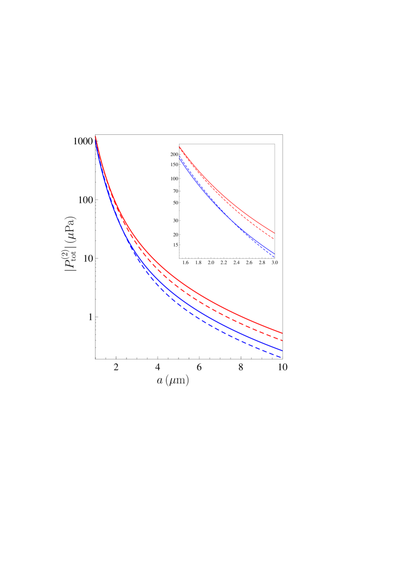
Figure 1: The magnitude of the total (Casimir) pressure on the lower Au plate kept at $T_{2}=500~{}$K is shown as a function of separation. The upper plate is kept at the temperature of the environment $T_{1}=300~{}$K. The top and bottom solid lines are computed using extrapolations of the optical data to low frequencies by means of the plasma and Drude models, respectively. The top and bottom dashed lines present the same quantity in the same way, but in thermal equilibrium $T_{1}=T_{2}=300~{}$K. The region near an intersection of the solid and dashed bottom lines is shown in more detail in an inset.

Now we use the resulting dielectric permittivities of Au along the imaginary frequency axis to calculate the Casimir pressure out of thermal equilibrium. We first consider the pressure $P_{\rm tot}^{(2)}$ acting on the lower Au plate kept at temperature $T_{2}$, which does not contain the separation-independent term. In order to clearly demonstrate the effect of thermal nonequilibrium, we choose $T_{1}=300~{}$K (as in the environment) and a rather large $T_{2}=500~{}$K. In Fig. 1 we plot the resulting magnitude of the (negative) nonequilibrium Casimir pressure as a function of separation, computed with the plasma (top solid line) and Drude (bottom solid line) models for extrapolation of the optical data of Au. As a comparison, we also plot the corresponding results for the equilibrium case ($T_{1}=T_{2}=300~{}$K) as the dashed lines, again using the plasma (top line) and Drude (bottom line) extrapolations, respectively.

As is seen in Fig. 1, the magnitudes of the Casimir pressure out of thermal equilibrium are larger than in equilibrium if the plasma model extrapolation is used. If, however, the Drude model extrapolation is used in computations, the bottom solid and dashed lines intersect, i.e., at short separations the magnitude of the nonequilibrium Casimir pressure is smaller than of the equilibrium one. To demonstrate this effect more clearly, we show the relevant separation range 1.5–$3~{}\mu$m in the inset. It is seen that if the Drude model is used an intersection between the solid and dashed lines takes place at $a\approx 2.3~{}\mu$m. As can be seen in Fig. 1, thermal nonequilibrium has a strong impact on the magnitude of the Casimir pressure.

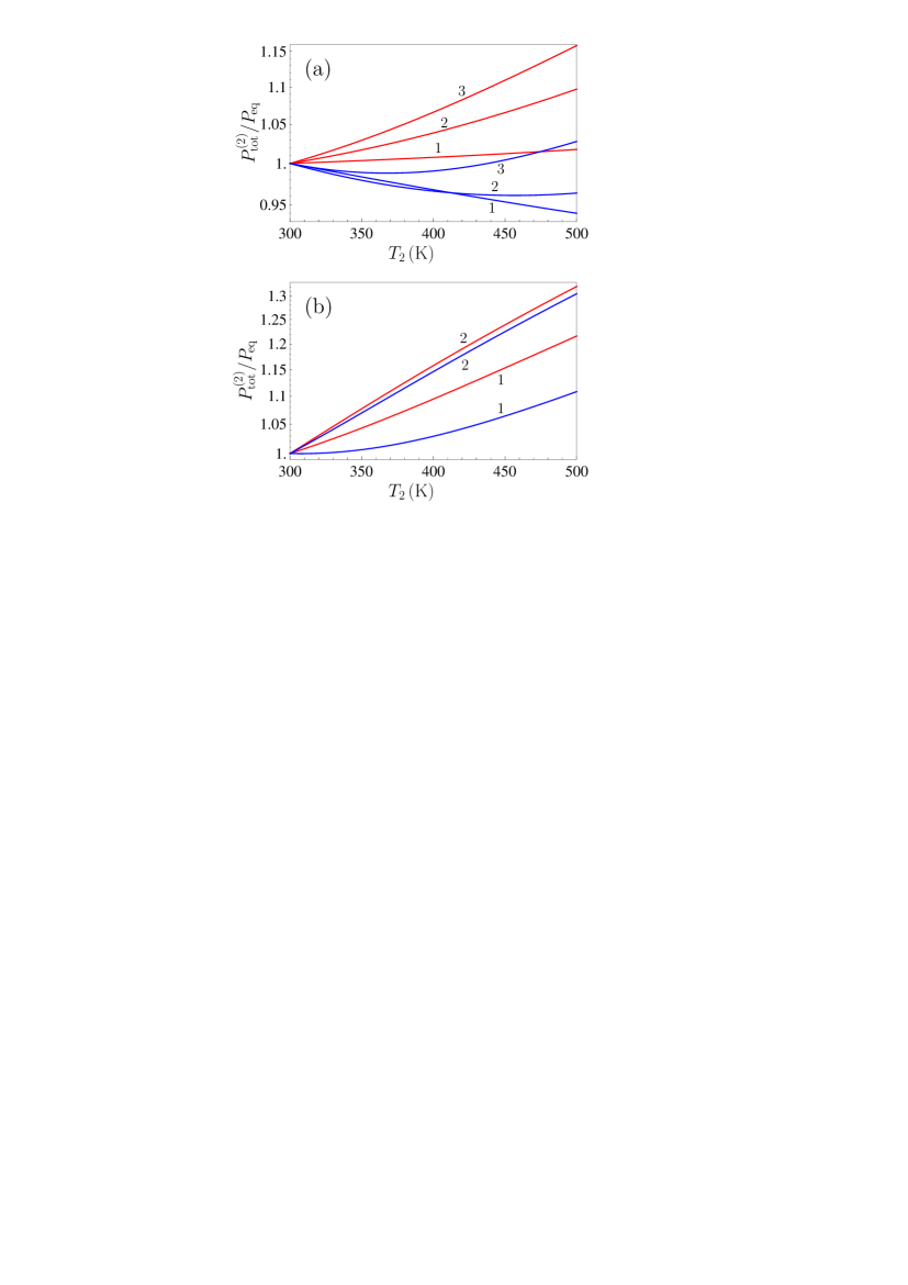
Figure 2: The total (Casimir) pressure on the lower Au plate, where the upper plate is kept at the temperature of the environment $T_{1}=300~{}$K, normalized by the Casimir pressure at thermal equilibrium, is shown by the pairs of lines labeled (a) 1, 2, and 3 and (b) 1 and 2 as a function of temperature $T_{2}$ of the lower plate. The pairs of lines are computed at separations between the plates (a) $a=1$, 2, and $2.5~{}\mu$m for the pairs labeled 1, 2, and 3 and (b) $a=3$ and $5~{}\mu$m for the pairs labeled 1 and 2, respectively. In each pair the top and bottom lines are computed using extrapolations of the optical data to low frequencies by means of the plasma and Drude models, respectively.

Now we calculate the nonequilibrium Casimir pressure $P_{\rm tot}^{(2)}$ as a function of the temperature $T_{2}$ of the lower plate with fixed $T_{1}=300~{}$K. The computational results are normalized by the Casimir pressure at equilibrium, $P_{\rm\!eq}$, computed at $T_{1}=T_{2}=300~{}$K and are shown in Fig. 2. The three pairs of lines labeled 1, 2, and 3 in Fig. 2(a) are plotted at separations $a=1$, 2, and $2.5~{}\mu$m, respectively. In so doing, the top line in each pair is computed using the plasma model extrapolation and the bottom one using the Drude model extrapolation. In a similar way, in Fig. 2(b) the two pairs of lines labeled 1 and 2 are plotted at $a=3$ and $5~{}\mu$m, and the top and bottom lines in each pair are computed using the plasma and Drude models, respectively.

As is seen in Fig. 2, the ratio $P_{\rm tot}^{(2)}/P_{\rm\!eq}$ monotonously increases with $T_{2}$ if the plasma model is used in computations. If, however, the Drude model is used, the quantity $P_{\rm tot}^{(2)}/P_{\rm\!eq}$ is nonmonotonous with increase of $T_{2}$ [see the bottom lines in Fig. 2(a)]. At all separations and temperatures there are significant differences between the computational results obtained using the plasma and Drude extrapolations of the optical data [note that although at $a=5~{}\mu$m the two solid lines labeled 2 in Fig. 2(b) deviate by only 1–2%, the theoretical predictions of the Lifshitz theory combined with either the Drude or the plasma models for both $P_{\rm tot}^{(2)}$ and $P_{\rm eq}$ differ by almost a factor of two].

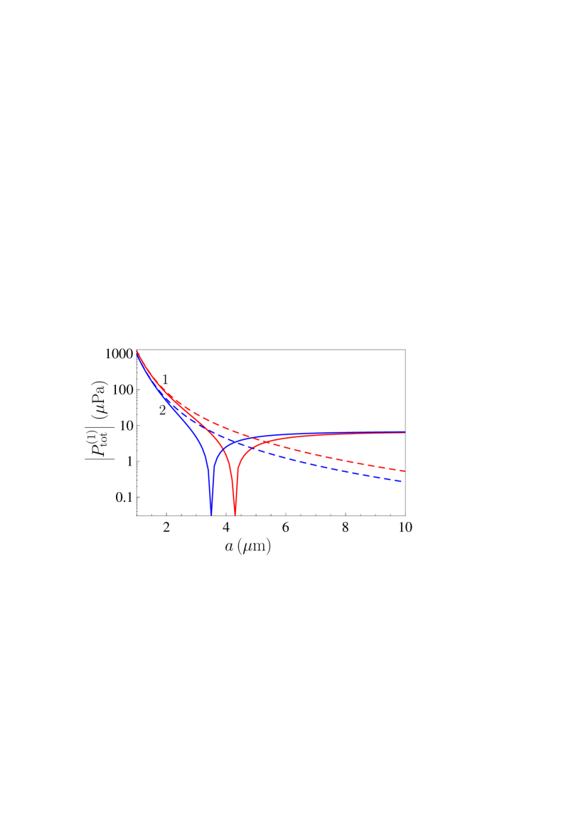
Figure 3: The magnitude of the total pressure on the upper plate in the configuration of two Au plates kept at $T_{1}=300~{}$K and $T_{2}=500~{}$K is shown as a function of separation by the two solid lines 1 and 2 computed using extrapolations of the optical data to low frequencies by means of the plasma and Drude models, respectively. The dashed lines 1 and 2 show the magnitude of the Casimir pressure on the lower Au plate computed using the plasma and Drude models.

Next, we consider the pressure on the upper plate which is in equilibrium with the environment at temperature $T_{1}$. It is given by Eq. (15). We put $T_{1}=300~{}$K equal to the temperature of the environment and $T_{2}=500~{}$K. The computational results as a function of separation are shown in Fig. 3 by the solid lines labeled 1 and 2, which are computed using extrapolations of the optical data by means of the plasma and Drude models, respectively. For comparison purposes, the dashed lines 1 and 2 show the magnitudes of the total pressure on the lower plate computed by Eq. (16) using the same respective extrapolations of the optical data (these dashed lines were already presented as the respective solid lines in Fig. 1). Note that for the upper plate the nonequilibrium pressure changes its sign from attractive to repulsive. This happens due to the presence of the last term on the right-hand side of Eq. (15). Thus, for each of the solid lines 1 and 2 in Fig. 3 the range of separations to the left of the respective minimum corresponds to the attraction (the force is negative), and to the right of the respective minimum corresponds to repulsion (the force is positive). The values of separation distances separating the ranges of attraction and repulsion are $a\approx 4.3$ and $3.5~{}\mu$m when the plasma and the Drude model extrapolations are used in computations, respectively.

IV Experimental test capable of discriminating between different theoretical approaches

In this section we suggest minor modifications in the experimental setup of the CANNEX test of the quantum vacuum, which was originally suggested for observation of thermal effects in the equilibrium Casimir force at large separations and constraining Yukawa-type corrections to Newton’s gravitational law and parameters of hypothetical particles 44 ; 45 ; 46 . We demonstrate that with these modifications CANNEX is most useful for a measurement of the nonequilibrium pressure considered in Secs. II and III and for a conclusive discrimination between different theoretical approaches to the account of free charge carriers.

IV.1 The modified CANNEX setup

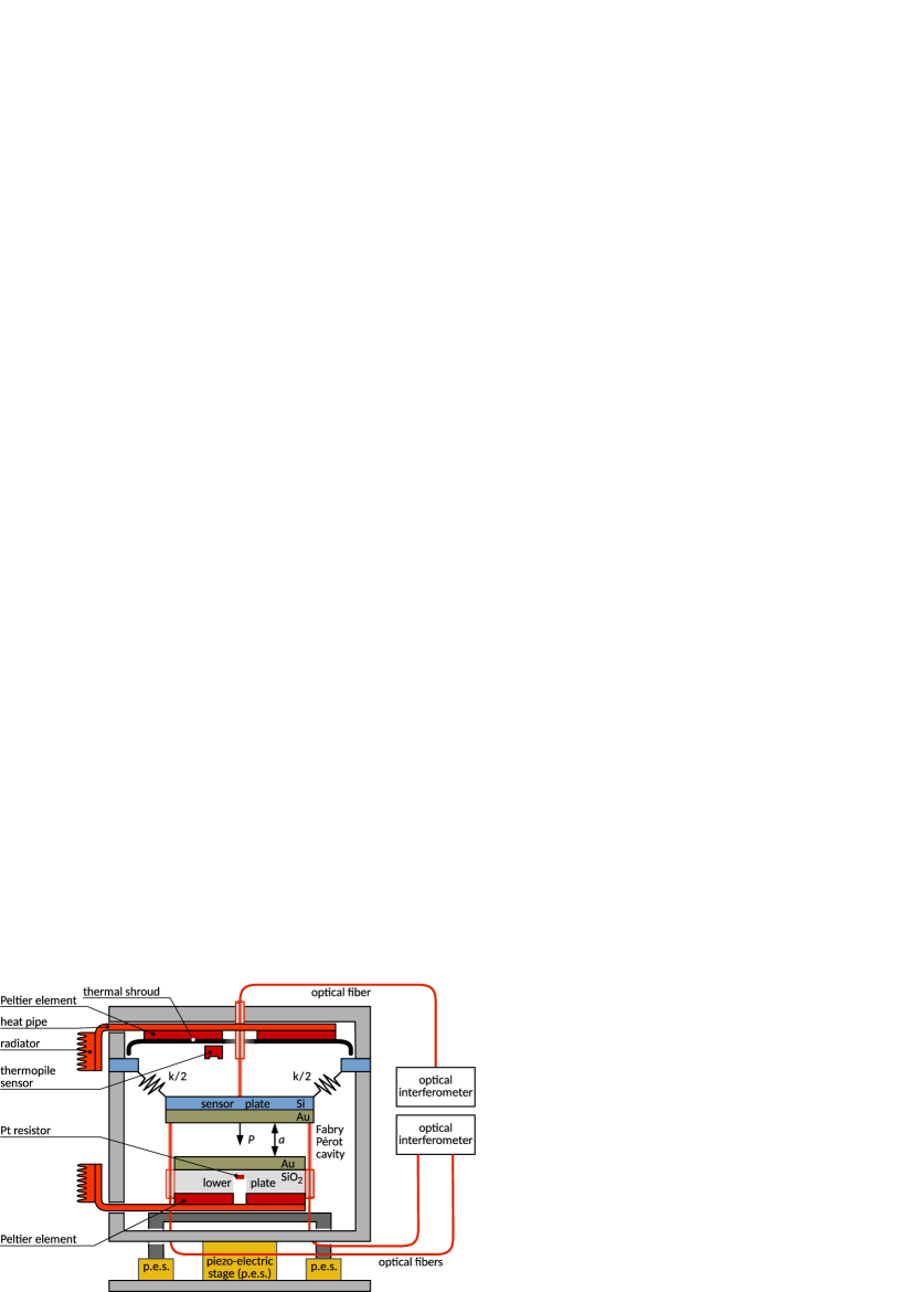
Figure 4: Simplified schematic of the modified experimental setup of the CANNEX test that allows for different temperatures on the sensor (upper) and lower plates by means of accurate feedback-controlled heating and cooling (see the text for further discussion). Shown not to scale.

CANNEX is an experimental setup for simultaneous measurements of the Casimir pressure and its gradient on the upper one of two parallel plates at separations from 3 or 4 to $15~{}\mu$m. The schematic of the setup is presented in Fig. 4. The upper (sensor) plate is a disc of $R=5.742$ mm radius consisting of a Si substrate of $100~{}\mu$m thickness and an Au film of thickness $d=200$ nm deposited on its bottom surface. The system of a sensor plate attached to three springs (only two of them are shown symbolically) is characterized by the elastic constant $k$ and effective mass $m_{\rm eff}$, and has the resonance frequency $\omega_{0}=(k/m_{\rm eff})^{1/2}$ 44 . The lower plate is formed by a vertical SiO₂ cylinder of 6 mm height coated with $1~{}\mu$m of Au. The entire setup is placed in a vacuum chamber (see Refs. 45 ; 46 for more details).

The pressure applied to the upper plate, as well as its gradient, are detected interferometrically in the experiment. Pressures are sensed by monitoring changes in the extension of the sensor’s springs, $\Delta a=\pi R^{2}P/k$. Pressure gradients are measured using a phase-locked loop that detects the shift $\Delta\omega$ of the resonance frequency under the influence of the total (Casimir) force 4 ; 13 ; 14 ; 45 . For this purpose, the lower three interferometers (again, only two of them are shown in the simplified scheme of Fig. 4) are used. The latter also monitor the separation distance $a$ at different positions around the rim of the lower plate, thereby allowing for an accurate determination and control of parallelism. As a result of several improvements in the setup suggested in Ref. 46 , sensitivities of the setup relative to the pressure and pressure gradient measurements will be improved to 1 nPa and 1 mPa/m, respectively.

In addition to the recent proposal 46 , we now present another modification of the CANNEX setup, allowing to increase the temperature of the lower plate by 10 K with no loss in the sensitivity. In fact, the improved sensitivities mentioned above require a temperature stability of the sensor better than $1\,$mK. For this reason, only the temperature of the lower plate may be varied, while the sensor plate has to be kept stable in temperature. This can practically be achieved by the thermal measurement and control scheme sketched in Fig. 4. The upper half of the sensor plate is connected radiatively to a thermal shroud mounted on a Peltier element. In order to monitor the sensor’s temperature, a contactless thermopile sensor is placed above the upper plate. On the lower side, the temperature of the fixed SiO₂ plate is measured near its surface via an embedded platinum resistor, and controlled by Peltier elements at its base.

At a controlled temperature of $T_{1}=300\,$K of the sensor plate and entire setup (which is the temperature of an environment), and a temperature $T_{2}=310~{}$K of the lower plate, the net radiative input to the sensor plate is just $129~{}\mu$W, thanks to the low thermal emission and absorption coefficient of gold ($\sim\,0.02$). The resulting temperature gradient over the thickness of the sensor is negligible. Moreover, as Si is almost transparent at wavelengths larger than the bandgap ($1.1~{}\mu$m) but has an emissivity of around 0.7 49 , the thermal shroud can be in perfect thermal contact with the sensor. Keeping the sensor at $T=T_{1}$ thus requires the shroud temperature to be roughly 301 mK below $T_{1}$. Excess heat can always be eliminated via heat pipes and radiators that interact with the inner wall of the vacuum chamber (not shown), which is temperature controlled with a precision of $1~{}$mK as well.

IV.2 Computational results in the experimental configuration

Now we compute the nonequlibrium total pressure and pressure gradient on the upper plate for the experimental parameters listed above including the values of temperature $T_{1}=300~{}$K and $T_{2}=310~{}$K, i.e., a rather moderate change, as compared to the equilibrium situation. It turns out, however, that this change is quite sufficient in order to observe the role of nonequilibrium in the measured quantities as well as to discriminate between different theoretical approaches to the description of relaxation using the CANNEX setup.

We start with the computation of the pressure gradient which is not sensitive to the presence of the third (separation-independent) term on the right-hand side of Eq. (12)

$${P_{\rm tot}^{(1)}}^{\,\prime}(a,T_{1},T_{2})=\frac{1}{2}[P_{\rm eq}^{\,\prime}(a,T_{1})+P_{\rm eq}^{\,\prime}(a,T_{2})]$$

$$~{}~{}~{}~{}~{}~{}~{}+\Delta P_{\rm neq}^{\,\prime}(a,T_{1},T_{2}).$$ (19)

Direct computations using Eqs. (7)–(10) show that although the parallel plates of CANNEX are dissimilar, with the experimental parameters $d_{1}=200$ nm and $d_{2}=1~{}\mu$m the contribution of the term $\Delta P_{\rm neq}^{\,\prime}$ on the right-hand side of Eq. (19) is by more than four orders of magnitude less than the contribution of the first term. This is explained by the fact that the thicknesses $d_{1}$ and $d_{2}$ are larger than the thermal wavelength contributing to $\Delta P_{\rm neq}^{\,\prime}$. Thus, in the experimental configuration the gradient of the total pressure on the upper plate can be computed by the equation

$${P_{\rm tot}^{(1)}}^{\,\prime}(a,T_{1},T_{2})=\frac{1}{2}[P_{\rm eq}^{\,\prime}(a,T_{1})+P_{\rm eq}^{\,\prime}(a,T_{2})],$$ (20)

where from Eq. (2) one obtains

$$P_{\rm eq}^{\,\prime}(a,T_{j})=\frac{k_{B}T_{j}}{8\pi a^{4}}\sum_{l=0}^{\infty}{\vphantom{\sum}}^{\prime}\int_{\zeta_{l}^{(j)}}^{\infty}y^{3}dy$$

$$~{}\times\sum_{\alpha}\left[\frac{e^{y}}{R_{\alpha}^{(1)}(i\zeta_{l}^{(j)}\!\!,y)R_{\alpha}^{(2)}(i\zeta_{l}^{(j)}\!\!,y)}-1\right]^{-2}\frac{e^{y}}{R_{\alpha}^{(1)}(i\zeta_{l}^{(j)}\!\!,y)R_{\alpha}^{(2)}(i\zeta_{l}^{(j)}\!\!,y)}.$$ (21)

Here, the reflection coefficients are defined in Eqs. (4)–(6).

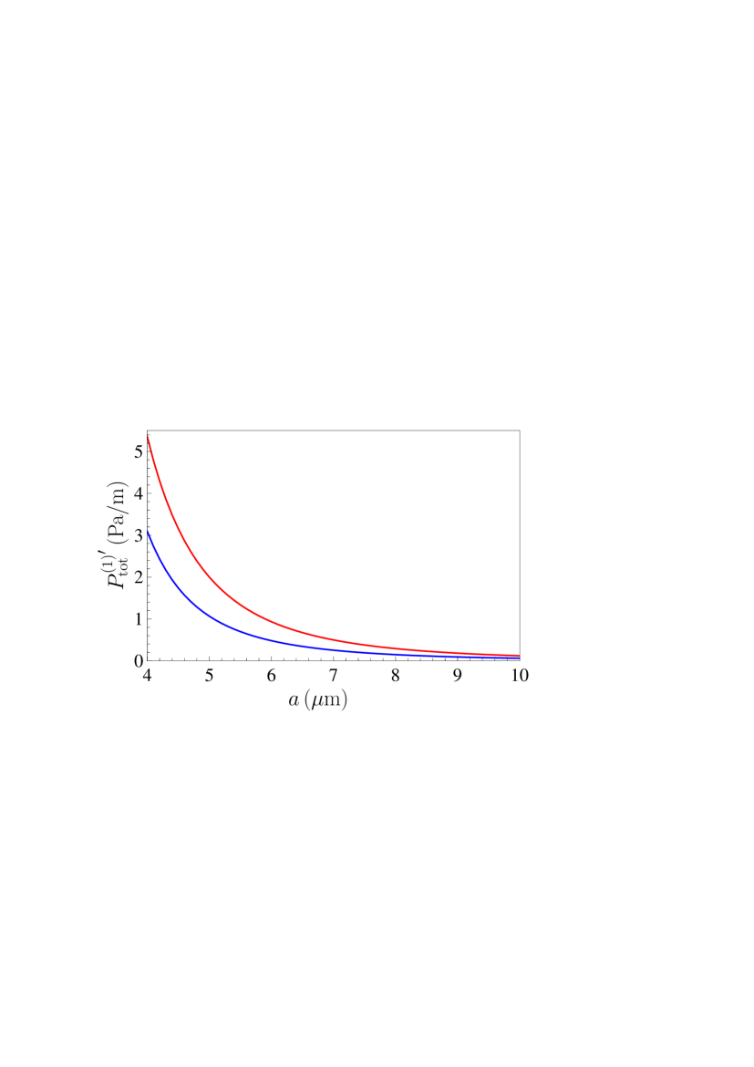
Figure 5: The gradient of the total pressure for the experimental parameters of CANNEX applied to the upper plate kept at $T_{1}=300~{}$K while the lower plate is heated to $T_{2}=310~{}$K is shown as a function of separation by the top and bottom lines computed using the extrapolations of the optical data to low frequencies by means of the plasma and Drude models, respectively.

In Fig. 5, we present computational results for the gradient of the total pressure applied to the upper plate for the experimental configuration. The top and bottom lines are obtained when the extrapolation of optical data of Au to low frequencies is performed by means of the plasma and Drude models, respectively. Note that with the experimental thicknesses $d_{1}$ and $d_{2}$ of the Au layers indicated above, the dielectric parts of the plates do not contribute to the result. As is seen in Fig. 5, within the separation region from 4 to $9~{}\mu$m the differences in the two theoretical predictions exceed the experimental sensitivity in measurements of the pressure gradient by a factor of $2\times 10^{3}$ to $10^{2}$. This means that the alternative theoretical approaches to the calculation of the pressure gradient can be easily discriminated in the experiment under consideration.

Now we discuss whether it is possible to discriminate the contribution due to different temperatures of the plates in the measurement results for the total nonequilibrium pressure gradient ${P_{\rm tot}^{(1)}}^{\,\prime}(a,T_{1},T_{2})$ given by Eq. (20). For this purpose we consider the differential pressure gradient

$${P_{\rm diff}^{(1)}}^{\,\prime}(a,T_{1},T_{2})={P_{\rm tot}^{(1)}}^{\,\prime}(a,T_{1},T_{2})-P_{\rm eq}^{\,\prime}(a,T_{1}),$$ (22)

where $T_{1}=300~{}$K, $T_{2}=310~{}$K.

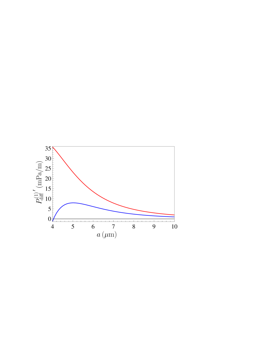
Figure 6: The differential gradient of the total pressure for the experimental parameters of CANNEX applied to the upper plate kept at $T_{1}=300~{}$K while the lower plate is heated to $T_{2}=310~{}$K is shown as a function of separation by the top and bottom lines computed using the extrapolations of the optical data to low frequencies by means of the plasma and Drude models, respectively.

The computational results for the quantity ${P_{\rm diff}^{(1)}}^{\,\prime}$ are shown in Fig. 6 as functions of separation. The top and bottom lines are computed using the plasma and Drude extrapolations of the optical data of Au to low frequencies, respectively. According to Sec. IV.A, the experimental sensitivity with respect to the difference of two pressure gradients is 2 mPa/m. As is seen in Fig. 6, the differential pressure gradients shown by the bottom line computed using the Drude extrapolation exceed the experimental sensitivity by up to a factor 4. However, the differential pressure gradients computed using the plasma extrapolation (the top line) exceed the experimental sensitivity by up to a factor 18. Thus, even for only 10 K temperature difference between the plates both the effect of nonequlibrium and the type of theoretical approach used for its description can be reliably determined.

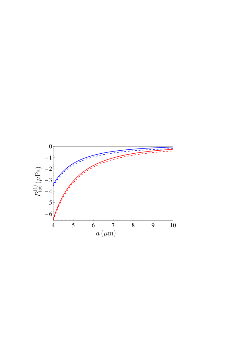
Figure 7: The total pressure for the experimental parameters of CANNEX applied to the upper plate kept at $T_{1}=300~{}$K while the lower plate is heated to $T_{2}=310~{}$K is shown as a function of separation by the top and bottom solid lines computed using the extrapolations of the optical data to low frequencies by means of the Drude and plasma models, respectively. Similar results computed with omitted separation-independent term are shown by the top and bottom dashed lines.

Now we return to the nonequlibrium total pressure given by Eq. (12) and consider potentialities of CANNEX as a test for the presence of separation-independent contributions. First, we calculate the pressure applied to the upper plate kept at $T_{1}=300~{}$K while the lower plate is kept at $T_{2}=310~{}$K. The computational results as functions of separation are shown in Fig. 7 where the top and bottom solid lines are computed using the Drude and plasma extrapolations of the optical data to low frequencies, respectively. Taking into account that the sensitivity of the CANNEX setup to pressure measurements is equal to 1 nPa, the alternative theoretical predictions can be easily discriminated experimentally over the entire separation range from 4 to $10~{}\mu$m shown in Fig. 7. The dashed lines in Fig. 7 show the respective computational results with omitted separation-independent term in Eq. (12). The difference between the solid and neighboring dashed lines is equal to $0.14~{}\mu$Pa and, thus, can be observed in the CANNEX experiment.

As is seen in Fig. 7, the presence of a separation-independent term in Eq. (15) does not lead to some qualitative changes in the total pressure. To demonstrate the role of this term in more detail, we consider the differential pressure applied to an upper plate

$$P_{\rm diff}^{(1)}(a,T_{1},T_{2})=P_{\rm tot}^{(1)}(a,T_{1},T_{2})-P_{\rm eq}(a,T_{1}).$$ (23)

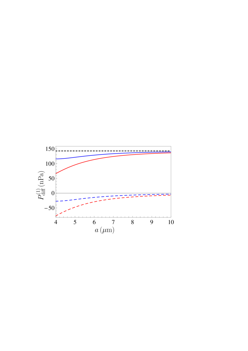
Figure 8: The differential pressure for the experimental parameters of CANNEX applied to the upper plate kept at $T_{1}=300~{}$K while the lower plate is heated to $T_{2}=310~{}$K is shown as a function of separation by the top and bottom solid lines computed using the extrapolations of the optical data to low frequencies by means of the Drude and plasma models, respectively. Similar results computed with the same parameters but omitted separation-independent term are shown by the top and bottom dashed lines for which $P_{\rm diff}<0$. The separation-independent contribution to the nonequilibrium pressure is indicated by the short-dashed line.

The computational results for the quantity $P_{\rm diff}^{(1)}$ are shown as functions of separation by the top and bottom solid lines in Fig. 8 obtained using the Drude and plasma models, respectively. The top and bottom dashed lines show the negative values of $P_{\rm diff}$, which would be obtained from $P_{\rm diff}^{(1)}$ using the Drude and plasma models, but with omitted constant term on the right-hand side of Eq. (15). The value of this term is indicated by the short-dashed line at the top of Fig. 8. The sensitivity of the CANNEX test to pressure differences $P_{\rm diff}$ is twice the one to pressure, i.e., 2 nPa. This means that differences between the top and bottom solid (dashed) lines in Fig. 8, as well as differences between the solid and dashed lines, can be easily discriminated by comparing the measurement results with theory. Because of this, the CANNEX test should be capable not only to discriminate between two different approaches to describe the relaxation properties of conduction electrons in nonequilibrium situations, but to validate or disprove the presence of separation-independent terms in the nonequlibrium Casimir pressure as well.

V Conclusions and discussion

In the foregoing we have proposed a novel test on the role of relaxation properties of free electrons in the out-of-equilibrium Casimir pressure between two parallel metal-coated plates kept at different temperatures – one of which is equal to the ambient temperature. It is shown that if the metallic coatings are sufficiently thick, the nonequilibrium pressures are determined by the mean of the equilibrium contributions calculated at two different temperatures and the term independent on separation between the plates. In this situation the temperature-antisymmetric contribution to the pressure is equal to zero with a high degree of accuracy. Thus, the proposed test represents an alternative to the previous suggestion 42 , which is directed to testing the role of relaxation properties in the latter, antisymmetric, contribution. In doing so, the other two contributions to the nonequlibrium pressure considered by us are screened out in Ref. 42 .

To demonstrate the role of the relaxation properties of conduction electrons in a nonequilibrium situation, computations of the Casimir pressure as a function of separation were performed for two parallel Au plates of finite thickness, where the upper plate is kept at ambient temperature $T_{1}=300~{}$K, and the temperature of the lower plate is $T_{2}=500~{}$K. The ratio of the Casimir pressures for thermal nonequilibrium and equilibrium was also investigated as a function of temperature of the lower plate varying from 300 to 500 K. In all cases computations have been made by using the extrapolations of the optical data of Au to low frequencies by means of both the plasma and Drude models. It was shown that the use of different extrapolations leads to markedly different theoretical predictions.

Furthermore, the experimental configuration of the CANNEX test, originally intended to measure the Casimir pressure and pressure gradient in the plane-parallel geometry in thermal equilibrium, was modified to allow for different temperatures on the two plates while preserving high experimental sensitivities. The nonequilibrium pressure, pressure gradient and contributions to these quantities due to different temperatures of the lower plate were computed in the experimental configuration using both the plasma and Drude models for extrapolations of the optical data to low frequencies. It was shown that even with a rather small difference of 10 K between the temperatures of the upper and lower plates, theoretical predictions for the total nonequilibrium pressure and pressure gradient, as well as for the terms independent on separation and contributions due to different temperatures, computed using the plasma and Drude models, can be reliably discriminated taking into account the experimental sensitivities.

Thus, the modified CANNEX test could be helpful in the resolution of the Casimir puzzle actively discussed in the literature for the last two decades. The situation in this problem is really challenging. The expression for the Casimir free energy was carefully derived from first principles in case of dissipation using different theoretical approaches including the fluctuation-dissipation theorem 12 ; 53 ; 54 ; 55 ; 56 ; 57 ; 58 . This means that it should be valid also in the case of the Drude model. In spite of this, in many direct measurements of the Casimir force and its gradient performed starting in 2003 (see Refs. 4 ; 13 for a review and more modern experiments 14 ; 15 ; 16 ; 17 ) the predictions of the Lifshitz theory with taken into account dissipation of free electrons were excluded at up to 99% confidence level. The predictions of the same theory with omitted dissipation of free electrons were confirmed. In these experiments, the measurement errors were equal to a fraction of a percent to compare with the difference between two theoretical predictions up to 5%. Based on this, the possible role of some unaccounted systematic effects was underlined by many authors. The situation has been changed after the proposed differential measurement scheme 59 where the predictions of the Lifshitz theory combined with the Drude and plasma models differ by up to a factor of 1000. After performing the respective experiment 18 , the Lifshitz formula combined with the Drude model was excluded with absolute certainty in spite of the fact that it seems to be well justified theoretically. The predictions of the Lifshitz theory combined with the plasma model were again found in good agreement with the measurement data.

A commonly accepted understanding of the roots of the problem is still missing. It is the authors’ opinion that they might go back to the foundations of quantum statistical physics. According to one of the postulates, the responses of a physical system to a real electromagnetic field possessing a nonzero strength and to a fluctuating field characterized by a zero strength but nonzero dispersion are similar. The dielectric response to a real field can be directly measured and is described by the Drude model as it is confirmed by abundant evidence. The dielectric response to a fluctuating field, however, can be observed only indirectly in phenomena such as the Casimir effect. Thus, the above mentioned postulate may be treated as a far reaching extrapolation which requires a reconsideration basing on the experimental results on measuring the Casimir interaction.

To conclude, the CANNEX test, originally proposed to measure the pressure and pressure gradient between parallel flat plates in equilibrium, may provide important additional information regarding the role of relaxation properties of conduction electrons in the out-of-equilibrium Casimir effect.

References

- (1) M. Kardar and R. Golestanian, The “friction” of vacuum and other fluctuation-induced forces, Rev. Mod. Phys. 71, 1233 (1999).
- (2) R. H. French, V. A. Parsegian, R. Podgornik, et al., Long-range interactions in nanoscale science, Rev. Mod. Phys. 82, 1887 (2010).
- (3) H. B. G. Casimir, On the attraction between two perfectly conducting plates, Proc. K. Ned. Akad. Wet. B 51, 793 (1948).
- (4) M. Bordag, G. L. Klimchitskaya, U. Mohideen, and V. M. Mostepanenko, Advances in the Casimir Effect (Oxford University Press, Oxford, 2015).
- (5) H. B. Chan, V. A. Aksyuk, R. N. Kleiman, D. J. Bishop, and F. Capasso, Quantum mechanical actuation of microelectromechanical systems by the Casimir force, Science 291, 1941 (2001).
- (6) R. Esquivel-Sirvent and R. Pérez-Pasqual, Geometry and charge carrier induced stability in Casimir actuated nanodevices, Eur. Phys. J. B 86, 467 (2013).
- (7) W. Broer, G. Palasantzas, J. Knoester, and V. B. Svetovoy, Significance of the Casimir force and surface roughness for actuation dynamics of MEMS, Phys. Rev. B 87, 125413 (2013).
- (8) M. Sedighi, W. H. Broer, G. Palasantzas, and B. J. Kooi, Sensitivity of micromechanical actuation on amorphous to crystalline phase transformations under the influence of Casimir forces, Phys. Rev. B 88, 165423 (2013).
- (9) W. Broer, H. Waalkens, V. B. Svetovoy, J. Knoester, and G. Palasantzas, Nonlinear Actuation Dynamics of Driven Casimir Oscillators with Rough Surfaces, Phys. Rev. Appl. 4, 054016 (2015).
- (10) L. Tang, M. Wang, C. Y. Ng, M. Nikolic, C. T. Chan, A. W. Rodriguez, and H. B. Chan, Measurement of nonmonotonic Casimir forces between silicon nanostructures, Nat. Photonics 11, 97 (2017).
- (11) G. L. Klimchitskaya, V. M. Mostepanenko, V. M. Petrov, and T. Tschudi, Optical Chopper Driven by the Casimir Force, Phys. Rev. Applied 10, 014010 (2018).
- (12) E. M. Lifshitz, The theory of molecular attractive forces between solids, Zh. Eksp. Teor. Fiz. 29, 94 (1955) [Sov. Phys. JETP 2, 73 (1956)].
- (13) G. L. Klimchitskaya, U. Mohideen, and V. M. Mostepanenko, The Casimir force between real materials: Experiment and theory, Rev. Mod. Phys. 81, 1827 (2009).
- (14) C.-C. Chang, A. A. Banishev, R. Castillo-Garza, G. L. Klimchitskaya, V. M. Mostepanenko, and U. Mohideen, Gradient of the Casimir force between Au surfaces of a sphere and a plate measured using an atomic force microscope in a frequency-shift technique, Phys. Rev. B 85, 165443 (2012).
- (15) A. A. Banishev, C.-C. Chang, G. L. Klimchitskaya, V. M. Mostepanenko, and U. Mohideen, Measurement of the gradient of the Casimir force between a nonmagnetic gold sphere and a magnetic nickel plate, Phys. Rev. B 85, 195422 (2012).
- (16) A. A. Banishev, G. L. Klimchitskaya, V. M. Mostepanenko, and U. Mohideen, Demonstration of the Casimir Force Between Ferromagnetic Surfaces of a Ni-Coated Sphere and a Ni-Coated Plate, Phys. Rev. Lett. 110, 137401 (2013).
- (17) A. A. Banishev, G. L. Klimchitskaya, V. M. Mostepanenko, and U. Mohideen, Casimir interaction between two magnetic metals in comparison with nonmagnetic test bodies, Phys. Rev. B 88, 155410 (2013).
- (18) G. Bimonte, D. López, and R. S. Decca, Isoelectronic determination of the thermal Casimir force, Phys. Rev. B 93, 184434 (2016).
- (19) V. B. Bezerra, G. L. Klimchitskaya, V. M. Mostepanenko, and C. Romero, Violation of the Nernst heat theorem in the theory of thermal Casimir force between real metals, Phys. Rev. A 69, 022119 (2004).
- (20) G. L. Klimchitskaya and C. C. Korikov, Analytic results for the Casimir free energy between ferromagnetic metals, Phys. Rev. A 91, 032119 (2015); 92, 029902(E) (2015).
- (21) G. L. Klimchitskaya and V. M. Mostepanenko, Low-temperature behavior of the Casimir free energy and entropy of metallic films, Phys. Rev. A 95, 012130 (2017).
- (22) S. M. Rytov, Theory of Electric Fluctuations and Thermal Radiation (Air Force Cambridge Research Center, Bedford, 1959).
- (23) D. Polder and M. Van Hove, Theory of radiative heat transfer between closely spaced bodies, Phys. Rev. B 4, 3303 (1971).
- (24) J. J. Loomis and H. J. Maris, Theory of heat transfer by evanescent electromagnetic waves, Phys. Rev. B 50, 18517 (1994).
- (25) A. I. Volokitin and B. N. J. Persson, Radiative heat transfer between nanostructures, Phys. Rev. B 63, 205404 (2001).
- (26) A. I. Volokitin and B. N. J. Persson, Resonant photon tunneling enhancement of the radiative heat transfer, Phys. Rev. B 69, 045417 (2004).
- (27) I. A. Dorofeyev, The force of attraction between two solids with different temperatures, J. Phys. A: Math. Gen. 31, 4369 (1998).
- (28) M. Antezza, L. P. Pitaevskii, and S. Stringari, New Asymptotic Behavior of the Surface-Atom Force out of Thermal Equilibrium, Phys. Rev. Lett. 95, 113202 (2005).
- (29) M. Antezza, L. P. Pitaevskii, S. Stringari, and V. B. Svetovoy, Casimir-Lifshitz Force Out of Thermal Equilibrium and Asymptotic Nonadditivity, Phys. Rev. Lett. 97, 223203 (2006).
- (30) M. Antezza, L. P. Pitaevskii, S. Stringari, and V. B. Svetovoy, Casimir-Lifshitz force out of thermal equilibrium, Phys. Rev. A 77, 022901 (2008).
- (31) G. Bimonte, Scattering approach to Casimir forces and radiative heat transfer for nanostructured surfaces out of thermal equilibrium, Phys. Rev. A 80, 042102 (2009).
- (32) R. Messina and M. Antezza, Scattering-matrix approach to Casimir-Lifshitz force and heat transfer out of thermal equilibrium between arbitrary bodies, Phys. Rev. A 84, 042102 (2011).
- (33) M. Krüger, T. Emig, and M. Kardar, Nonequilibrium Electromagnetic Fluctuations: Heat Transfer and Interactions, Phys. Rev. Lett. 106, 210404 (2011).
- (34) G. Bimonte, T. Emig, M. Krüger, and M. Kardar, Dilution and resonance-enhanced repulsion in nonequilibrium fluctuation forces, Phys. Rev. A 84, 042503 (2011).
- (35) M. Krüger, T. Emig, G. Bimonte, and M. Kardar, Nonequilibrium Casimir forces: Spheres and sphere-plate, Europhys. Lett. 95, 21002 (2011).
- (36) R. Messina and M. Antezza, Casimir-Lifshitz force out of thermal equilibrium and heat transfer between arbitrary bodies, Europhys. Lett. 95, 61002 (2011).
- (37) M. Krüger, G. Bimonte, T. Emig, and M. Kardar, Trace formulas for nonequilibrium Casimir interactions, heat radiation, and heat transfer for arbitrary bodies, Phys. Rev. B 86, 115423 (2012).
- (38) R. Messina and M. Antezza, Three-body radiative heat transfer and Casimir-Lifshitz force out of thermal equilibrium for arbitrary bodies, Phys. Rev. A 89, 052104 (2014).
- (39) A. Noto, R. Messina, B. Guizal, and M. Antezza, Casimir-Lifshitz force out of thermal equilibrium between dielectric gratings, Phys. Rev. A 90, 022120 (2014).
- (40) I. Latella, P. Ben-Abdallah, S.-A. Biehs, M. Antezza, and R. Messina, Radiative heat transfer and nonequilibrium Casimir-Lifshitz force in many-body systems with planar geometry, Phys. Rev. B 95, 205404 (2017).
- (41) A. I. Volokitin and B. N. J. Persson, Near-field radiative heat transfer and noncontact friction, Rev. Mod. Phys. 79, 1291 (2007).
- (42) B.-S. Lu, D. S. Dean, and R. Podgornik, Out-of-equilibrium thermal Casimir effect between Brownian conducting plates, Europhys. Lett. 112, 20001 (2015).
- (43) G. Bimonte, A Theory of Electromagnetic Fluctuations for Metallic Surfaces and van der Waals Interaction between Metallic Bodies, Phys. Rev. Lett. 96, 160401 (2006).
- (44) V. B. Bezerra, G. Bimonte, G. L. Klimchitskaya, V. M. Mostepanenko, and C. Romero, Thermal correction to the Casimir force, radiative heat transfer, and an experiment, Eur. Phys. J. C 52, 701 (2007).
- (45) G. Bimonte, Observing the Casimir-Lifshitz force out of thermal equilibrium, Phys. Rev. A 92, 032116 (2015).
- (46) Y.-J. Chen, W. K. Tham, D. E. Krause, D. López, E. Fischbach, and R. S. Decca, Stronger Limits on Hypothetical Yukawa Interactions in the 30–8000 nm Range, Phys. Rev. Lett. 116, 221102 (2016).
- (47) F. Chen, G. L. Klimchitskaya, U. Mohideen, and V. M. Mostepanenko, New Features of the Thermal Casimir Force at Small Separations, Phys. Rev. Lett. 90, 160404 (2003).
- (48) A. Almasi, P. Brax, D. Iannuzzi, and R. I. P. Sedmik, Force sensor for chameleon and Casimir force experiments with parallel-plate configuration, Phys. Rev. D 91,102002 (2015).
- (49) R. Sedmik and P. Brax, Status Report and first Light from Cannex: Casimir Force Measurements between flat parallel Plates, J. Phys.: Conf. Ser. 1138, 012014 (2018).
- (50) G. L. Klimchitskaya, V. M. Mostepanenko, R. I. P. Sedmik, and H. Abele, Prospects for Searching Thermal Effects, Non-Newtonian Gravity and Axion-Like Particles: CANNEX Test of the Quantum Vacuum, Symmetry 11, 407 (2019).
- (51) G. L. Klimchitskaya and V. M. Mostepanenko, Observability of thermal effects in the Casimir interaction with graphene-coated substrates, Phys. Rev. A 89, 052512 (2014).
- (52) M. S. Tomaš, Casimir force in absorbing multilayers, Phys. Rev. A 66, 052103 (2002).
- (53) C. Raabe, L. Knóll, and D.-G. Welsch, Three-dimensional Casimir force between absorbing multilayer dielectrics, Phys. Rev. A 68, 033810 (2003).
- (54) E. D. Palik (ed.), Handbook of Optical Constants of Solids (Academic Press, New York, 1985).
- (55) H. Sugawara, T. Ohkubo, T. Fukushima, and T. Iuchi, Emissivity Measurement of Silicon Semiconductor Wafer near Room Temperature, in: SICE 2003 Annual Conference IEEE Cat. No. 03TH8734, vol. 2, p.2201 (2003).
- (56) I. E. Dzyaloshinskii, E. M. Lifshitz, and L. P. Pitaevskii, The general theory of van der Waals forces, Usp. Fiz. Nauk 73, 381 (1961) [Adv. Phys. 10, 165 (1961)].
- (57) S. J. Rahi, T. Emig, N. Graham, R. L. Jaffe, and M. Kardar, Scattering theory approach to electrodynamic Casimir forces, Phys. Rev. D 80, 085021 (2009).
- (58) F. S. S. Rosa, D. A. R. Dalvit, and P. W. Milonni, Electrodynamic energy absorption and Casimir forces: Uniform dielectric media in thermal equilibrium, Phys. Rev. A 81, 033812 (2010).
- (59) F. Intravaia and R. Behunin, Casimir effect as a sum over modes in dissipative systems, Phys. Rev. A 86, 062517 (2012).
- (60) M. Bordag, Casimir and Casimir-Polder forces with dissipation from first principles, Phys. Rev. A 96, 062504 (2017).
- (61) R. Guérout, G.-L. Ingold, A. Lambrecht, and S. Reynaud, Accounting for Dissipation in the Scattering Approach to the Casimir Energy, Symmetry 10, 37 (2018).
- (62) G. Bimonte, Hide It to See It Better: A Robust Setup to Probe the Thermal Casimir Force, Phys. Rev. Lett. 112, 240401 (2014).