Ramifications of disorder on active particles in one dimension

Abstract

The effects of quenched disorder on a single and many active run-and-tumble particles is studied in one dimension. For a single particle, we consider both the steady-state distribution and the particle’s dynamics subject to disorder in three parameters: a bounded external potential, the particle’s speed, and its tumbling rate. We show that in the case of a disordered potential, the behavior is like an equilibrium particle diffusing on a random force landscape, implying a dynamics that is logarithmically slow in time. In the situations of disorder in the speed or tumbling rate, we find that the particle generically exhibits diffusive motion, although particular choices of the disorder may lead to anomalous diffusion. Based on the single-particle results, we find that in a system with many interacting particles, disorder in the potential leads to strong clustering. We characterize the clustering in two different regimes depending on the system size and show that the mean cluster size scales with the system size, in contrast to non-disordered systems.

1 Introduction

Self-propelled or active particles consume and dissipate energy in order to move persistently. The breaking of time-reversal symmetry by the drive, specially in the vicinity of external boundaries, leads to a plethora of interesting phenomena, distinct from those in equilibrium systems. For example, E. Coli. bacteria swim in circles near planar surfaces [1], and the motion of active particles is generally rectified by asymmetric objects [2, 3]. The latter effect generates currents, which in turn lead to long-range interactions between objects immersed in an active fluid [4]. Closely related is the fact that, in general, the mechanical pressure exerted on confining boundaries does not follow an equation of state and, on the contrary, depends on the details of the interactions with the boundary [5, 6, 7] and its curvature [8, 9].

So far, the bulk of studies have focused on the physics of active systems in the absence of disorder, namely in uniform environments. However, natural environments of many active agents, such as bacteria in the gut or enzymes in the intracellular medium [10], are non-uniform. While several recent studies have considered the effects of disorder on models of flocking [11, 12, 13, 14], comparatively less is known for the simpler case of non-aligning active particles subject to different types of quenched disorder. Such systems are realized experimentally [15] (and of course numerically [16]) using, for example, optical speckle fields or non-smooth substrates.

To this end, in this paper we consider run-and-tumble particles (RTPs) in a one-dimensional (quenched) disordered environment. This model of active particles has the advantage of allowing for exact calculations since one can write explicit expressions for the steady-state distributions and first passage times of non-interacting RTPs [17, 5]. We discuss three types of quenched disorder: in the external potential $V(x)$ which is assumed to be bounded, in the speed of the particles $v(x)$, and in their tumbling rate $\alpha(x)$. The main results are summarized in Table 1.

Most interestingly, a RTP in a bounded random potential is akin to a passive Brownian particle in a random force field. This leads to a strongly localized steady-state probability distribution, with the location of the maximum of the distribution depending on the exact shape of the potential throughout the system. Moreover, it exhibits the so-called Sinai diffusion [18] (reviewed in [19]) with logarithmically slow spreading in time. Interestingly, similar behavior has also been predicted for molecular motors which are stalled by an external force [20, 21]. We remind the reader that in stark contrast, a passive particle in a bounded random potential shows normal diffusion with a steady-state probability distribution which is uniform on large length-scales.

The strong clustering of the probability distribution also has a striking effect on interacting RTPs in the presence of a disordered potential. It is known that in one dimension RTPs with repulsive interactions form clusters of finite size [22, 23]. Here we argue using simplified models that the picture is very different. We analyze the problem in two regimes, defined below, which we refer to as weak and strong disorder. In the weak disorder case, we show that the density-density correlation function decays linearly in space with an amplitude which is linear in the system size. In the strong disorder regime we argue for a power-law distribution of cluster sizes, with the average cluster size scaling as the square root of the system size.

When the disorder enters through the particle’s speed, the steady-state probability distribution is generically uniform on large length-scales and the spreading is diffusive in time. An interesting exception occurs when the speed distribution is singular near zero (see Table 1). Then, the steady-state distribution is peaked at a specific location, with a height which grows as a power law in the system size. The probability distribution in this case spreads with anomalous time exponents.

Finally, for a disordered tumbling rate, the steady-state probability distribution is flat and the spreading is generically diffusive. Similar to the speed disorder, the spreading is anomalous when the tumbling distribution decays to zero with fat tails for large values of $\alpha$ (see Table 1).

The paper is organized as follows: we first consider a single particle in Section 2, deriving the steady-state distributions in Section 2.1 and dynamical properties in Section 2.2. The results of Section 2 are summarized in Table 1. Next, we turn to the many-body case, which we study using simplified models in Section 3. The discussion is carried for weak disorder in Section 3.1 and strong disorder in Section 3.2. Finally, we conclude and discuss the expected results of the disorder on higher dimensional systems and other active models in Section 4.

Disordered	Steady-state distribution,	Mean-square displacement
parameter	for a given realization of disorder
$V(x)$	$\frac{1}{1-\left(\frac{\mu}{v}\right)^{2}\left(\partial_{x}V\right)^{2}}\times$	$\overline{\left<x^{2}\right>}\sim\log^{4}\left(t\right)$
	$\exp\left(-\frac{\alpha\mu}{v^{2}}\intop^{x}\textrm{d}x^{\prime}\,\frac{\left(\partial_{x^{\prime}}V\right)}{1-\left(\frac{\mu}{v}\right)^{2}\left(\partial_{x^{\prime}}V\right)^{2}}\right)$
$v(x)$	$\frac{1}{v(x)}$	$p(v)\underset{v\to 0}{\to}0:$	$\overline{\left<x^{2}\right>}\sim t$
		$p(v)\underset{v\to 0}{\sim}v^{-\beta},\ 0<\beta<1:$	$\overline{\left<x^{2}\right>}\sim t^{1-\beta}$
$\alpha(x)$	const.	$p(\alpha)\underset{\alpha\to\infty}{\sim}0:$	$\overline{\left<x^{2}\right>}\sim t$
		$p(\alpha)\underset{\alpha\to\infty}{\sim}\alpha^{-(1+\mu)},\ 0<\mu<1:$	$\overline{\left<x^{2}\right>}\sim t^{\frac{2\mu}{1+\mu}}$

Table 1: Summary of results for the single particle problem: For each form of disorder, the steady-state distribution is given for a specific realization, along with the scaling of the variance of the probability density in time. The mean-square displacement is averaged both over histories of the dynamics, denoted by $\langle\cdot\rangle$, and over all realizations of the disorder, denoted by $\overline{\,\cdot\,}$.

2 Single-particle problem

We consider a Run-and-Tumble Particle (RTP) in one dimension. The particle moves either to the right or to the left with a speed $v(x)$ and switches direction (tumbles) at rate $\alpha(x)/2$. We allow both the speed and tumbling rate to depend on the position $x$ of the particle. Finally, the particle experiences an external potential $V(x)$. The probability density $P_{+}(x,t)$ ($P_{-}(x,t)$) to find a right (left) moving particle at position $x$ at time $t$ is determined by the Fokker-Planck equation [24, 25, 26]

$$\partial_{t}P_{+}(x,t)= -\partial_{x}\left[v(x)P_{+}(x,t)-\mu(\partial_{x}V)P_{+}(x,t)\right]-\frac{\alpha(x)}{2}\left[P_{+}(x,t)-P_{-}(x,t)\right]\ ,$$

$$\partial_{t}P_{-}(x,t)= -\partial_{x}\left[-v(x)P_{-}(x,t)-\mu(\partial_{x}V)P_{-}(x,t)\right]-\frac{\alpha(x)}{2}\left[P_{-}(x,t)-P_{+}(x,t)\right]\;,$$ (1)

with $\mu$ the mobility of the particle. To avoid trivial trapping, we assume that $v(x)>|\mu\partial_{x}V|$. This condition can be avoided if, in addition, the particle is subject to Brownian noise. The noise can assist the particle in hopping over potentials of arbitrary slope [27]. However, as we discuss in Sec. 4, we do not expect fundamentally new physics in this case, and we thus consider only the technically simpler noiseless situation.

We next consider the effect of disorder on the steady-state distribution in Section 2.1 and on the dynamics in Section 2.2. In each case, we focus on the three different types of disorder: in the potential, the speed and the tumbling rate.

2.1 Steady-state distributions

For the dynamics of Eq. (1), the steady-state distribution can be computed analytically [17, 5]. One starts by defining the total probability density $\rho(x,t)=P_{+}(x,t)+P_{-}(x,t)$ and the polarity $\Delta(x,t)=P_{+}(x,t)-P_{-}(x,t)$. Using Eq. (1), we have

$$\partial_{t}\Delta(x,t)= -\partial_{x}\left[v(x)\rho(x,t)-\mu(\partial_{x}V)\Delta(x,t)\right]-\alpha(x)\Delta(x,t)\ ,$$

$$\partial_{t}\rho(x,t)= -\partial_{x}\left[v(x)\Delta(x,t)-\mu(\partial_{x}V)\rho(x,t)\right]\ .$$ (2)

Assuming that the system is confined, so that there is no particle current in the steady state, one finds for a given realization of $\alpha(x),\,v(x)$ and $V(x)$ that the steady-state density $\rho_{s}(x)$ is given by

$$\rho_{s}(x)=\frac{{\cal N}v(x)}{v^{2}(x)-\mu^{2}\left(\partial_{x}V\right)^{2}}\exp\left(-\intop_{0}^{x}\textrm{d}x^{\prime}\,\frac{\alpha(x^{\prime})\mu\left(\partial_{x^{\prime}}V\right)}{v^{2}(x^{\prime})-\mu^{2}\left(\partial_{x^{\prime}}V\right)^{2}}\right)\ ,$$ (3)

where ${\cal N}$ is a normalization constant set by $\intop\textrm{d}x\,\rho_{s}(x)=1$. Equation (3) allows for variations in the potential $V(x)$, the speed $v(x)$ and the tumbling rate $\alpha(x)$. Figure 1 shows the resulting density if each component acts individually. It is easy to see from the figures that different types of disorder lead to very different behaviors: disorder in the potential has the strong effect of localizing the probability distribution to several locations in space; disorder in the velocity leads to a local modulation of the density which depends on the local velocity; while disorder in the tumbling rate leads to a flat steady-state distribution. In the following, we discuss these three cases in more detail.

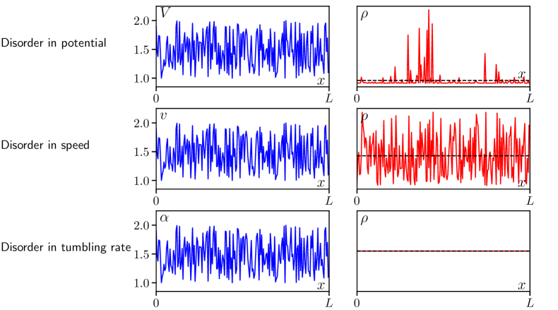
Figure 1: Steady-state distributions (right column) for the disorder profiles shown in the left column (for system size $L=200$). Top row: $v=2$, $\alpha=40$; middle and bottom rows: $V=0$.

2.1.1 Disordered potential

We first consider a disordered potential $V(x)$ while maintaining constant speed $v(x)=v$ and tumbling rate $\alpha(x)=\alpha$. As stated above, we choose the potential such that $|\mu\partial_{x}V|<v$ so that the particle can cross any potential barrier. Let us first rewrite Eq. (3) in terms of $\tilde{V}(x)\equiv\mu V(x)/v$ (so that the force $\partial_{x}\tilde{V}$ is dimensionless), and the inverse run length $g\equiv\alpha/v$, as

$$\rho_{s}\left(x\right)=\frac{{\mathcal{N}_{p}}}{1-\left(\partial_{x}\tilde{V}\right)^{2}}\exp\left(-g\intop_{0}^{x}\textrm{d}y\,\frac{\partial_{y}\tilde{V}}{1-\left(\partial_{y}\tilde{V}\right)^{2}}\right)$$ (4)

with $\mathcal{N}_{p}$ ensuring normalization. We further assume that $V(x)$ has only short-range correlations and denote its correlation length by $\xi$. We can then approximate the integral in Eq. (4) as a sum of independent identically distributed (i.i.d.) random variables

$$\intop_{0}^{x}\textrm{d}y\,\frac{\partial_{y}\tilde{V}}{1-\left(\partial_{y}\tilde{V}\right)^{2}}\approx\sum_{i=1}^{\lfloor x/\xi\rfloor}\eta_{i}\ .$$ (5)

The full justification of the above approximation can be found e.g. in [28]. To discuss the resulting stationary distribution, it is instructive to rewrite Eq. (4) as an equilibrium distribution $\rho_{s}(x)\propto e^{-U(x)}$ with the quasi-potential

$$U(x)\approx\ln\left[1-\left(\partial_{x}\tilde{V}\right)^{2}\right]+g\sum_{i=1}^{\lfloor x/\xi\rfloor}\eta_{i}\ .$$ (6)

Since the sum in Eq. (6) is over i.i.d. random variables, the quasi-potential scales as $U(L)\propto\sqrt{L/\xi}$ by virtue of the central limit theorem, given that the system is large enough $L\gg\xi$. For such systems, the quasi potential is dominated by the sum over the random variables and the logarithmic local term is negligible. At the level of the steady-state distribution, the behavior is thus identical to that of a passive particle in a random force field, with $g\eta_{i}/\xi$ as the random force. For any realization of such a random force, as in Fig. 1 (top row), the particle is strongly localized to the minima of the quasi-potential, which are of order $\sqrt{L}$.

The difference between the passive and active cases is therefore dramatic: an active particle in a bounded random potential is equivalent to a passive particle in a random force field. By contrast, a passive particle in a bounded random potential $V(x)$ does not show localization. The difference due to the activity can be understood intuitively as follows: since RTPs break time reversal symmetry, the particle exerts a net force on a potential lacking inversion symmetry (this effect was used experimentally to propel asymmetric objects through a bacterial bath [29, 30]). Conversely, the external potential exerts a net force on the RTP so that a random potential will effectively lead to a net random force [9]. For example, if we choose a particularly simple realization of the potential, where ratchet potentials of opposing directionality are drawn with equal probability, as illustrated in Fig. 2, the orientation of each ratchet biases the active particle in a particular direction acting as a local force. We note that similar physics applies for other ratchet-like systems [20, 21].

The model of a random walker subject to random forcing is known as the Sinai diffusion problem, and has been studied extensively in the past with many applications [18, 31, 19, 32]. In Section 2.2.1 we show that the equivalence between active particles in a random potential and passive particles in random force field also extends to the particle’s dynamics.

2.1.2 Disordered speed

We now consider systems where the disorder enters only through a space-dependent speed $v(x)$, while the tumbling rate $\alpha$ is constant and there is no external potential. We take $v(x)$ to be a random field taking values in the range $0<v(x)<\infty$, with only short-range correlations and a probability distribution independent of space. For a particular realization of the disorder, Eq. (3) becomes

$$\rho_{s}(x)=\frac{\mathcal{N}_{v}}{v(x)}\ ,$$ (7)

where $\mathcal{N}_{v}$ insures the normalization of the distribution. We note that such systems have been extensively studied in the past [25, 26] and used experimentally to draw patterns using photokinetic bacteria [33, 34].

Evidently, the active particle density is enhanced in places where the speed of the particles is smaller. However, in contrast with the case of a random potential discussed above, the steady-state distribution of the random speed model is a local function of $v(x)$ (whereas Eq. (4) shows that the density is a non-local functional of the potential). The resulting distribution (7), while non-uniform, is therefore not strongly localized in general. The particles show similar statistics as an equilibrium system subject to a random potential, $U(x)=-\ln v(x)$, with a finite variance.

An exception occurs when $v(x)$ takes values arbitrarily close to zero. In particular, consider a probability distribution for $v$ that vanishes as $p(v)\underset{v\to 0}{\sim}v^{-\beta}$ close to $0$. When $0<\beta<1$ the mean of $v^{-1}$ diverges. Then, using standard arguments from Lévy statistics, the largest value of $v^{-1}$ in a system of size $L$ scales as $L^{\frac{1}{1-\beta}}$. The particle becomes localized at the position of the maximal value of $v^{-1}$, with a probability scaling in the same way. Note that the non-uniformity of $\rho_{s}(x)$ is due to the singular distribution of velocities, and is not a cumulative effect of a non-local dependence on $v(x)$.

2.1.3 Disordered tumbling rate

Finally, we consider quenched disorder only in the tumbling rate. We take $\alpha(x)$ to be a random field which takes values in the range $0<\alpha(x)<\infty$ with short-range correlations, independent of space. Then, using Eq. (3) with $\partial_{x}V=0$, $v(x)=v$ we immediately get

$$\rho_{s}(x)=\text{constant}=\frac{1}{L}.$$ (8)

Disorder in $\alpha$ leaves the steady-state distribution flat.

2.2 Dynamics through the mean first passage time

Figure 2: A realization of the ratchet potential used in the numerics. The two possible orientations of each ratchet are chosen with equal probability.

We now turn to analyze the effects of disorder on the dynamics of active particles. This is most easily accomplished by considering the typical, disorder-averaged, mean first passage time (MFPT) for a particle to travel a distance $L$ in either direction starting at an arbitrary point. As we show below, the insights gained by studying the steady-state distribution can also be extended to the dynamics. Specifically, disorder in the potential leads to behavior similar to a random walker on a random forcing energy landscape. We show in Section 2.2.1 that the typical MFPT grows exponentially with $L^{\frac{1}{2}}$. This leads to an ultra-slow diffusive dynamics of the particle with a typical mean-square displacement growing in time as $\ln^{4}(t)$.

In contrast, disorder in the speed or tumbling rate generally leads to a behavior similar to equilibrium dynamics of a random walker in a bounded random potential. The MFPT averaged over the disorder follows a standard diffusion law, and grows as $L^{2}$. As discussed in Section 2.1.2, an exception occurs for a disordered speed distribution in which the mean inverse speed, $\overline{v^{-1}}$, over disorder realizations diverges, and for disordered tumbling rates when the mean tumbling rate $\overline{\alpha}$ diverges. These cases exhibit anomalous behavior, with the disorder-averaged mean-square displacement scaling with a non-trivial power of time.

2.2.1 Disordered potential

We now evaluate the typical MFPT for an active run-and-tumble particle in a random potential with uniform speed and tumbling rate. We consider a particle starting at an arbitrary point, taken to be $x=0$, and exiting either at $x=L$ or $x=-L$. Similar to the calculation for the steady-state distribution, we define the quasi-potential

$$W(x)=\frac{\mu\alpha}{v^{2}}\intop_{-L}^{x}\textrm{d}y\,\frac{\partial_{y}V}{1-\left(\frac{\mu}{v}\right)^{2}\left(\partial_{y}V\right)^{2}}.$$ (9)

Using the derivation presented in Appendix A.1, one finds that in the large $L$ limit the MFPT, up to exponentially smaller corrections in $L$, is given by

$$\left<\tau\right>\underset{L\rightarrow\infty}{\sim}\frac{\intop_{-L}^{0}\textrm{d}x\,\intop_{0}^{L}\textrm{d}y\,\intop_{x}^{y}\textrm{d}z\,Q(x)Q(y)Q(z)\exp\left[-W(x)-W(y)+W(z)\right]}{\intop_{-L}^{L}\textrm{d}u\,Q(u)\exp\left[-W(u)\right]}\ .$$ (10)

Here, $\langle\tau\rangle$ is the MFPT for a given realization of disorder, with the angular brackets denoting an average over histories, $Q(x)$ is a non-vanishing function whose expression is given in Appendix A.1 and, as will become clear, does not influence the leading order behavior.

Since the potential $V(x)$ is assumed to have short-range correlations, $W(x)$ is a sum of i.i.d. random variables. Note that since the integrand in $W(x)$ is anti-symmetric with respect to inverting $\partial_{y}V(x)$ to $-\partial_{y}V(x)$, the average of $W(x)$ over the realizations of the disorder vanishes. The central limit theorem then gives the behavior of $W(x)$ in the large $L$ limit: the distribution of $W(x)$ converges asymptotically to a Gaussian distribution, whose variance scales as $\sqrt{L/\xi}$, with $\xi$ being the correlation length of $V(x)$, as before. In the large $L$ limit, the MFPT is therefore dominated by the exponential term and can be evaluated using a saddle-point approximation. One then finds

$$\ln\langle\tau\rangle\underset{L\rightarrow\infty}{\sim}-\min_{x\in[-L,0],y\in[0,L],\,z\in[x,y]}\left[W(x)+W(y)-W(z)\right]+\min_{u\in[-L,L]}\left[W(u)\right]\ .$$ (11)

Even if the MFPT (11) has a non-trivial dependance on the potential, it is clear that its asymptotic behavior in the large $L$ limit is of the order of the largest difference of the effective potential $W(x)$ in the $[-L,L]$ interval.

Note that for a given realization of the disorder, the MFPT is controlled by an exponentially large quantity in the potential difference. Therefore, there is a difference between the average MFPT and the typical one. The latter is of interest and is encoded in the disorder average of $\ln\langle\tau\rangle$ given in Eq. (11). This gives

$$\overline{\ln\left<\tau\right>}\underset{L\rightarrow\infty}{\sim}A\sqrt{L}\ ,$$ (12)

where $A$ is a constant that depends on the details of the potential $W(x)$.

The above result indicates that the mean-square displacement of an active particle on a random potential behaves as

$$\overline{\langle x^{2}(t)\rangle}\underset{t\rightarrow\infty}{\propto}\ln^{4}(t)$$ (13)

where $x(t)$ is the displacement at time $t$. This indicates that the dynamics of the active particle on a one dimensional random potential energy landscape is an ultra-slow Sinai diffusion. Indeed, at the exponential level, the MFPT of the two models is identical. We verify this prediction numerically in Fig. 3 for the random ratchet model illustrated in Fig. 2: the disorder-averaged mean-square displacement as a function of time for active RTP on a disordered random ratchet potential agrees with Eq. (13) in the long-time limit.

It is interesting to ask when the effects of a weak random potential become important. To study this question we appeal to the equilibrium random forcing analogy. In this case, a natural length scale [19] for the crossover is given by $\ell^{*}\simeq D^{2}/\sigma^{2}$ with $D$ the diffusivity of the particle and $\sigma^{2}$ the variance of the random force. Namely, $\overline{f(x)f(x^{\prime})}=\sigma^{2}\delta(x-x^{\prime})$, with $f(x)$ the force at position $x$. In the active case $D=v^{2}/\alpha$, while $\sigma^{2}$ depends on the details of the potential distribution. The value of $\sigma^{2}$, which depends in a non-trivial way on the parameters of the model and cannot be easily evaluated, is a measure of the strength of the ratchet effect for a given disorder distribution. Therefore, as expected, the stronger ratchets lead to shorter crossover lengths (see Fig. 3). Note that the same length scale can be obtained from Eq. (4) by considering the quasi-potential. In analogy with a Boltzmann weight, the temperature scale $T$ is set by the ratio $\sigma\sqrt{L}/D$, where $D=v^{2}/\alpha$. The low temperature regime then corresponds to the strong disorder limit $L\gg\ell^{*}$ while the high temperature limit corresponds to systems where $L\ll\ell^{*}$ and the density profile is to leading order uniform.

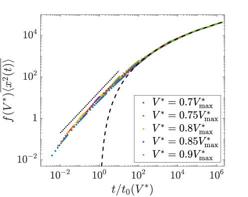
Figure 3: Dynamics of active particles on random ratchet potentials of varying strength. Different plots correspond to ratchets which differ only by their maximal height, $V^{*}$, with a slope ratio of 1:4. Heights are given relative to the maximal ratchet height $V^{*}_{\rm max}$ which imposes a slope $|\mu\partial_{x}V|=v$. Such slope prevents the particle from moving. For each $V^{*}$, 100 RTPs are simulated on a potential of $10^{4}$ ratchets for $10^{7}$ time steps, with unit mobility and speed. The time and mean-square displacement are rescaled by constants so that the data collapse for long times. The dashed line marks the theoretical prediction of Eq. (13) $\overline{\langle x^{2}(t)\rangle}\propto\ln^{4}(t)$, showing good agreement on long times with the numerical data. The dotted line shows the diffusive scaling $\overline{\langle x^{2}(t)\rangle}\propto t$, valid for short times. For stronger $V^{*}$, the numerical curves approach the disorder dominated regime earlier.

2.2.2 Speed disorder

We now turn to the dynamics of active particles in the presence of a spatially varying speed. The difference in steady-state distributions between this case and that of random potentials was already emphasized in Sec. 2.1.2. To proceed, we note, using the results from Appendix A.2, that when the disorder enters through the speed, the MFPT is asymptotically given by

$$\left<\tau\right>\underset{L\rightarrow\infty}{\sim}\frac{\alpha\intop_{-L}^{0}\textrm{d}x\,\,\intop_{-L}^{L}\textrm{d}y\,\intop_{x}^{y}\textrm{d}z\,v^{-1}(x)v^{-1}(y)v^{-1}(z)}{\intop_{-L}^{L}\textrm{d}z\,v^{-1}(w)}\ .$$ (14)

This expression will be analyzed in two distinct cases. In the first, the speed probability density vanishes near $v=0$, while in the second the probability density diverges near $v=0$.

Case I: vanishing probability density near $\mathbf{v=0}$. In this case, the dynamics is diffusive. The denominator of Eq. (14) in the large $L$ limit is well approximated, due to the law of large numbers, by $2L\overline{v^{-1}}$. Then, the disorder average of $\langle\tau\rangle$ can readily be evaluated. The leading order term in the numerator is given by the product of the disorder averages of the inverse speed, scaling as $L^{3}$, with corrections scaling as $L^{2}$. To see this, one defines $v^{-1}=\overline{v^{-1}}+\delta v^{-1}$ and assumes short-range correlations of the deviations $\delta v^{-1}$ in space. This leads to diffusive behavior,

$$\overline{\left<\tau\right>}\underset{L\rightarrow\infty}{\sim}\frac{\alpha}{2}\left(\overline{v^{-1}}\right)^{2}L^{2}\ ,$$ (15)

as verified numerically in Fig. 4.

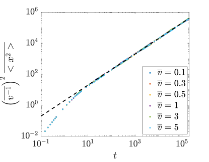
Figure 4: Dynamics of active particles with varying speed, randomly drawn at each point from a uniform distribution in the interval $[0.9\overline{v},1.1\overline{v}]$. The plots are for 100 particles and $10^{8}$ time steps, 1000 realizations of disorder, 6 mean speeds and a unit tumbling rate. The disorder-averaged variance of the probability distribution, rescaled according to Eq. (15), is plotted as a function of time. The dashed line is fitted to diffusive motion, $\overline{\langle x^{2}(t)\rangle}\sim t$.

Case II: diverging probability density near $\mathbf{v=0}$. Here we assume that the probability density near $v=0$ takes the form $p(v)\sim v^{-\beta}$, with $0<\beta<1$. It is well known that slow bonds can lead to anomalous diffusive behavior [35], and a similar phenomenon also occurs here. To evaluate the MFPT (14), we note that the dependence of the denominator on $L$ can be obtained using standard properties of Lévy distributions [19]. The integral of the denominator of Eq. (14) is dominated by the largest value of $v^{-1}$ on the interval of length $L$, denoted by $(v^{*})^{-1}$, which scales as $(v^{*})^{-1}\approx L^{\frac{1}{1-\beta}}$. Similarly, the numerator is dominated by the largest contribution to each of the integrals, scaling as $L^{\frac{3}{1-\beta}}$. The resulting MFPT is then given by

$$\overline{\left<\tau\right>}\underset{L\rightarrow\infty}{\propto}\frac{\alpha}{2}L^{\frac{2}{1-\beta}}\ .$$ (16)

This anomalous diffusion is verified numerically in Fig. 5. Finally, we note that the results suggests that when $\beta=0$, one should expect $\overline{\langle\tau\rangle}\propto L^{2}/\log(L)$.

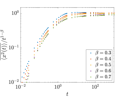
Figure 5: The disorder-averaged spreading for randomly distributed speed (case II), rescaled with time as suggested by Eq. (16). The dynamics of active particles is simulated with speeds varying in space, drawn from the distribution $p(v)\sim v^{-\beta}$ in the interval $[0,1]$, for 100 particles $10^{5}$ time steps, 1000 realizations of disorder, and unit tumbling rate.

2.2.3 Tumbling rate disorder

Finally, let us consider the dynamics of the active particle in the presence of a tumbling rate that varies in space. This was shown in Section 2.1.3 to have no effect on the steady-state distribution, leading to a flat density profile.

Using the results of Appendix A.2, to leading order in $L$ the MFPT is given by

$$\langle\tau\rangle\underset{L\to\infty}{\sim}\frac{1}{v^{2}}\frac{\intop_{-L}^{0}\textrm{d}x\,\intop_{0}^{L}\textrm{d}y\,(y-x)\alpha(x)\alpha(y)}{\intop_{-L}^{L}\textrm{d}z\,\alpha(w)}\ .$$ (17)

As in the case of the speed disorder, we distinguish here between two limits.

Case I: probability density with a finite mean. Here, we can use an integration by part to transform Eq. (17) into

$$\langle\tau\rangle\underset{L\to\infty}{\sim}\frac{1}{v^{2}}\frac{\intop_{-L}^{0}\textrm{d}x\,\intop_{0}^{L}\textrm{d}y\,\left(\alpha(x)\intop_{y}^{L}\textrm{d}z\,\alpha(z)+\alpha(y)\intop_{-L}^{x}\textrm{d}z\,\alpha(z)\right)}{\intop_{-L}^{L}\textrm{d}z\,\alpha(w)}\ .$$ (18)

Then using the law of large numbers and arguments almost identicals to those leading to Eq. (15), we find that the MFPT is given by

$$\overline{\left<\tau\right>}\underset{L\rightarrow\infty}{\sim}\frac{\overline{\alpha}}{2v^{2}}L^{2}\ .$$ (19)

Namely, the dynamics is diffusive, as verified numerically in Fig. 6.

Case II: probability density with a diverging mean. To evaluate the expression for the MFPT (17), we use the arguments presented in Case II of the speed disorder, taking $p(\alpha)\sim\alpha^{-(1+\mu)}$ for large $\alpha$ with $0<\mu<1$. Doing so, we find that the denominator scales as $L^{1/\mu}$ while the numerator as $L^{1+2/\mu}$. This leads to

$$\overline{\langle\tau\rangle}\underset{L\rightarrow\infty}{\propto}\frac{1}{2v^{2}}L^{1+1/\mu}\ ,$$ (20)

a result verified numerically in Fig. 7.

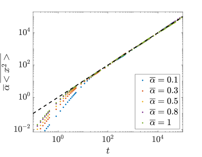
Figure 6: Dynamics of active particles with a random tumbling rate varying in space (case I). The tumbling rate is drawn from a uniform distribution in $[0,2\overline{\alpha}]$, for 100 particles, $10^{8}$ time steps, 1000 realizations of disorder, 5 mean tumbling rates, and a unit speed. The disorder-averaged variance of the probability distribution, rescaled according to Eq. (19), is plotted as a function of time. The curves are fitted with diffusive dynamics, i.e. $\overline{\langle x^{2}(t)\rangle}\sim t$.

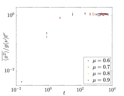
Figure 7: The disorder-averaged spreading for a disordered tumbling rate (case II), rescaled by time according to Eq. (20). Here $\nu=2\mu/(1+\mu)$, and the rescaling factor $g(\nu)$ is chosen so that the curves asymptotically approach the same value. The dynamics of active particles is simulated with a random tumbling rate varying in space, drawn from the distribution $p(\alpha)\sim\alpha^{-(1+\mu)}$ for $\alpha\in(0,\infty)$, for 100 particles, $10^{6}$ time steps, 1000 realizations of disorder, and unit speed.

3 Many RTPs in a disordered potential

As shown in the previous section, a RTP in a disordered potential behaves as a random walker on a random-forcing energy landscape. This implies that the particle feels an effective potential whose depth grows as $\sqrt{L}$ with the system size $L$. In this section we consider the consequences of this fact for the many-body problem with a finite density of particles, for both interacting and non-interacting RTPs. Recall that for a single RTP in a disordered potential, there is a length scale $\ell^{*}$ (see Sec. 2.2.1), below which the motion is diffusive and above which the motion is logarithmically slow. Accordingly, the discussion that follows is carried out separately for systems for which $L<\ell^{*}$, referred to as weak disorder, and with $L>\ell^{*}$, referred to as strong disorder.

Most strikingly, we find that the presence of disorder promotes order in these systems. In the case of weak disorder, the two-point correlation function is shown, using numerics and a simplified theory, to decay linearly in space with an amplitude scaling linearly with the system size $L$. In the case of strong disorder with no interactions, as expected, the particles accumulate around a single minimum leading to a correlation function which decays over a finite distance. For the interacting case, it is well known that in the absence of disorder RTPs in one dimension only exhibit clusters of finite extent [22, 23]. In contrast, here we find that the cluster size distribution is distributed as a power-law with a mean cluster size which scales as $\sqrt{L}$.

3.1 Weak disorder

As explained above, we start by considering systems for which $L<\ell^{*}$. In this limit, the density profile of the system is expected to be approximately uniform with small fluctuations. Recalling that RTPs on a random potential are equivalent to Brownian particles on a random forcing energy landscape, we consider the simplified free energy functional

$$\mathcal{F}=\intop\textrm{d}x\,\left[\frac{K}{2}\left(\partial_{x}\phi\right)^{2}+\frac{u}{2}\phi^{2}(x)+\phi(x)U(x)\right]\;.$$ (21)

Here, the field $\phi(x)$ represents the density fluctuations from the mean value; $K$ accounts for interactions; $u$ contains both the leading order interaction and entropic contributions; while $U(x)$ is a random potential with the statistics of a random forcing energy landscape,

$$\begin{cases}\overline{U(x)}=0,\\ \overline{U(x)U(y)}=\frac{\sigma^{2}}{2}(x+y-|x-y|)\;.\end{cases}$$ (22)

Throughout this section, we use the convention $f_{q}=\frac{1}{\sqrt{L}}\int_{0}^{L}\textrm{d}x\,f(x)e^{-iqx}$ for the Fourier transform of any function $f(x)$ defined on the interval $[0,L]$, e.g. with $\phi_{q}$ as the Fourier component $q$ of the density deviation field.

To characterize the effects of disorder, we focus on the disorder-averaged structure factor

$$\overline{S(q)}=\overline{\langle\phi_{q}\phi_{-q}\rangle}\,,$$ (23)

with the overline, as before, denoting the average over disorder realizations and the brackets indicating averages over the probability distribution governed by the Boltzmann weight from Eq. (21). Since this weight is Gaussian, one can easily calculate exactly the disorder-averaged structure factor: The partition function $\mathcal{Z}$ for a given realization of the disorder is given by

$$\ln\mathcal{Z}=\underset{q}{\sum}\,\left[\frac{1}{2u}\frac{U_{q}U_{-q}}{\left(1+\frac{K}{u}q^{2}\right)}-\ln\left(Kq^{2}+u\right)\right]\ ,$$ (24)

where $U_{q}$ are the Fourier modes of the random potential. To compute the structure factor we first evaluate

$$\langle\phi_{q}\phi_{-q}\rangle_{c}=\frac{\delta}{\delta U_{q}}\frac{\delta}{\delta U_{-q}}\ln\mathcal{Z}\ ,$$ (25)

with $\langle\phi_{q}\phi_{-q}\rangle_{c}=\langle\phi_{q}\phi_{-q}\rangle-\langle\phi_{q}\rangle\langle\phi_{-q}\rangle$ the connected correlation function. Then, noting that

$$\langle\phi_{q}\rangle=\frac{1}{u}\frac{U_{q}}{\left(1+\frac{K}{u}q^{2}\right)}\ ,$$ (26)

we arrive at the two-point correlation function for a given realization of disorder as

$$S(q)=\frac{1}{u\left(1+\frac{K}{u}q^{2}\right)}\left[1+\frac{1}{u}\frac{U_{q}U_{-q}}{\left(1+\frac{K}{u}q^{2}\right)}\right]\ .$$ (27)

After averaging over realizations of disorder, we obtain

$$\overline{S(q)}=\frac{1}{u\left(1+\frac{K}{u}q^{2}\right)}\left[1+\frac{1}{u}\frac{\overline{U_{q}U_{-q}}}{\left(1+\frac{K}{u}q^{2}\right)}\right].$$ (28)

Using Eq. (22) to compute the correlation $\overline{U_{q}U_{-q}}$, we finally get for $q\neq 0$

$$\overline{S(q)}=\frac{1}{u\left(1+\frac{K}{u}q^{2}\right)}+\frac{2\sigma^{2}}{q^{2}u^{2}(1+{\frac{K}{u}q^{2}})^{2}}.$$ (29)

To leading order in the $q\rightarrow 0$ limit, one finds $\overline{S(q)}\propto q^{-2}$ signalling that there are long-range correlations in the system. Note that this behavior is a consequence of the correlations in the potential, which are manifested even in the non-interacting case $K=0$, with $u$ accounting for purely entropic contributions. In real space, Eq. (29) gives the asymptotic behavior for large $r$

$$\overline{S(r)}=\frac{1}{L}\intop_{0}^{L}\textrm{d}x\,\overline{\langle\phi(x)\phi(x+r)\rangle}\propto L\left(1-A\frac{r}{L}\right),$$ (30)

with $A$ an amplitude. The $\big{(}\frac{r}{L}\big{)}$ decay of Eq. (30) shows that the correlations decay linearly with a scale proportional to the system size – a result reminiscent of a phase separated system. This suggests that a macroscopic number of particles accumulate around the deepest part of the potential.

Note that for $r=0$, we find that $\frac{1}{L}\int_{0}^{L}\textrm{d}x\,\overline{\phi^{2}(x)}\propto L$. This relation suggests a non-trivial scaling of the typical magnitude of the density fluctuations. To understand this scaling we note that the interaction term $\frac{u}{2}\phi^{2}(x)$ in the free energy accounts for repulsion between the particles and is balanced by the term $\phi(x)U(x)$, which tends to gather particles at the minimum of the potential. This minimum scales as $\sqrt{L}$, and so the typical magnitude of the density fluctuations in the dense phase scales in the same way.

We now compare the field-theoretic result with numerical simulations of RTPs in the ratchet potential of Fig. 2. We simulate, at the same average density of $\rho_{0}=0.25$, both non-interacting particles and particles interacting via a short-range pairwise harmonic repulsion $U_{r}(\Delta)=\frac{k}{2}(1-\Delta)^{2}$ if $\Delta<1$ and $U_{r}=0$ otherwise, with $\Delta$ the inter-particle separation. The results are presented in Fig. 8. As predicted by the field theory, we find, for both interacting and non-interacting particles, that the structure factor diverges as $q^{-2}$ at small $q$. For each case, two different sizes are plotted in Fig. 8 to check that the scaling of the structure factor with $L$ is consistent with the one given in Eq. (29).

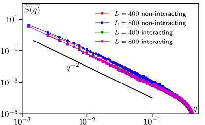
Figure 8: Structure factor in the weak disorder case, with ratchets of height $V^{*}=0.58V^{*}_{\rm max}$. $V^{*}_{\rm max}$ is defined as the potential height which creates a slope $|\mu\partial_{x}V|=v$ which stops the particle. Interacting particles experience a short-range interaction of strength of $k=10$. The average density $\langle\rho\rangle=0.25$ is simulated on a ring of length $L=800$, with particles of unit speed, tumbling rate, and mobility.

3.2 Strong disorder

Here we consider the strong disorder limit where the system size obeys $L\gg\ell^{*}$, with $\ell^{*}$ the crossover length scale between the standard and ultra-slow diffusive regimes. Since numerical simulations proved prohibitively slow in this regime, we employ simple heuristic arguments building on the analogy between RTPs in a random potential and Brownian particles in a random forcing energy landscape. As we argue, unlike the weak disorder limit, the phenomenology is now very different between interacting and non-interacting particles.

For the non interacting case, there is no bound on the maximal density at each point in space. At low enough temperatures $T\ll\sigma L^{\frac{1}{2}}$, non-interacting particles can all collapse around the location of the global minimum of $U$ (as defined in Eq. (6)), and the fluctuations are expected to be confined to a finite region around it. This leads to the expected behavior of the density-density correlation function

$$\overline{{\cal S}(r)}=\frac{1}{L}\intop_{0}^{L}\textrm{d}x\,\overline{\langle\rho(x)\rho(x+r)\rangle}\sim Lf(r),$$ (31)

where $\rho(r)$ is the density at $r$, and $f(r)$ is a function that decays on a length scale independent of the length $L$. As stated above, in the strong disorder regime, the convergence to the steady state proved too slow to obtain numerical results. We therefore use the analogy derived in section 2.1.1 between active particles in a random potential and passive particles in a random forcing energy landscape. To this end, we use a potential defined on a lattice, such that the energy difference between adjacent sites is a random variable taking the values $\pm 1$ (in arbitrary units) and therefore corresponds to a random force. For non-interacting Brownian particles in a random-forcing energy landscape, the steady-state distribution is then given by the usual Boltzmann distribution $\rho_{s}(x)\propto e^{-U(x)/T}$, and can readily be evaluated. (Recalling the discussion at the end of Sec. 2.2.1 we note that the strong disorder regime corresponds to low temperatures, and thus the Gaussian form emerging from Eq. (21) is no longer applicable in this limit.) Evaluating the steady-state distribution numerically, we find that as long as the temperature is low enough, the correlation functions indeed behave as expected from Eq. (31) (see Fig. 9). This implies that essentially all the particles collapse near the minimal energy.

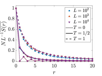
Figure 9: The disorder-averaged two-point function $\overline{S(r)}=L^{-1}\intop_{0}^{x}\textrm{d}x\,\overline{\langle\rho(x)\rho(x+r)\rangle}$ divided by the system size $L$ in real space, with periodic boundary conditions. To verify the scaling of Eq. (31), the correlation function is rescaled by $L$ and plotted for different system sizes and temperatures of the random forcing equilibrium model. Since for non-interacting particles the overall density $\rho_{0}$ enters as a trivial $\rho_{0}^{2}$ factor, we take $N$ such that $NL^{-1}\overline{S(r)}$ so that it is unity at $r=0$. Note that the oscillations in the $T=0$ curves are due to degenerate minima.

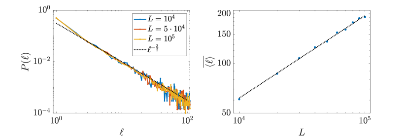
Figure 10: Left: Distribution of cluster sizes for for interacting RTPs, with the same mean density as Fig. 9 and different system sizes. The distribution is extracted from $10^{3}$ disorder realizations of the random forcing energy landscape. The curves are fitted with a probability distribution, scaling as $\ell^{-\frac{3}{2}}$. Right: Average cluster size as a function of the system size, plotted along with the theoretical prediction of Eq. (33), $\overline{\langle\ell\rangle}\propto\sqrt{L}$.

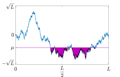
Figure 11: Particles with hard-core repulsion filling a realization of the random forcing energy landscape, at $T=0$. The particles occupy all energies up to the chemical potential, $\mu$, which controls the mean density, here set to $\langle\rho\rangle=0.4$.

We again employ the analogy to Brownian particles in a random forcing potential to understand the case of interacting RTPs. For simplicity we assume that the particles are on a lattice with hard-core interactions. Such particles can be treated as non-interacting Fermions with a chemical potential $\mu$ setting their overall number. Clusters are defined as sequences of particles with no vacancies and the distribution of cluster sizes is shown in Fig. 10 (left). (Since the overall energy scale, set by the chemical potential, is much larger than the effective temperature we consider the zero temperature limit of this model.) Interestingly, the domain size distribution, $P(\ell)$ behaves as a power-law

$$P(\ell)\sim\frac{1}{\ell^{3/2}}\;,$$ (32)

implying that the average domain size in the system grows as

$$\langle\ell\rangle\sim\sqrt{L}\;,$$ (33)

as verified in Fig. 10 (right). The origin of the power-law distribution of cluster sizes can be understood by considering Fig. 11, in which the chemical potential, controlling the filled locations on the lattice, is marked explicitly for a given realization of the disorder. It is clear that the size of a cluster is dictated by the statistics of first return of a random walk, starting and ending at the chemical potential, which is indeed governed by Eq. (32).

We end this section by noting that it is straightforward to numerically obtain the two-point correlation function, $\overline{{\cal S}(r)}$ (see Fig. 12). Simple theoretical arguments using the self-similarity of the Brownian motion show that for a fixed particle density, the two-point correlation function is a function of $\big{(}\frac{r}{L}\big{)}$. However, we have not been able to obtain explicit analytical expressions for this functional form. The problem is related to statistics of extrema of random walks (see for example [36, 37] where the problem is properly defined but still unsolved) and is beyond the scope of this manuscript.

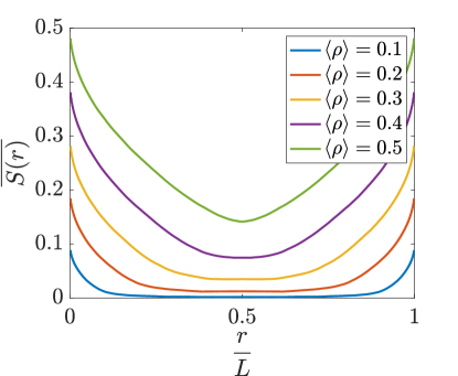
Figure 12: The disorder-averaged two-point function $\overline{S(r)}=L^{-1}\intop_{0}^{x}\textrm{d}x\,\overline{\langle\rho(x)\rho(x+r)\rangle}$ in real space, with periodic boundary conditions. The curves correspond to different average densities, $\langle\rho\rangle$.

4 Summary

In this paper we studied active particles in disordered one-dimensional environments. Considering the effects of three types of disorder (in the external potential, the speed, and the tumbling rate), we derived the steady-state distributions and dynamical properties for a single run-and-tumble particle. In the case of potential disorder, we also consider the many-body case with either interacting or non-interacting particles.

In the single-particle problem, the most striking manifestation of disorder was obtained for random potentials: The active particles were shown to exhibit ultra-slow Sinai diffusion at long times, a behavior analogous to passive random walkers on a random forcing energy landscape. In the paper, we considered run-and-tumble particles with no translational diffusion and were therefore restricted to potentials with limited slope. If translational diffusion is allowed, the particles can hop across steep local barriers, as recently analyzed in Ref. [27]. Using these results, it is easy to see that a local forcing is still present in this case when the barrier lacks an inversion symmetry. Therefore, the conclusion drawn from the case analyzed in the bulk of this paper remains unchanged. Similarly, any 1d active particle model where ratchet currents are generated should exhibit the same phenomenology.

For disordered speed and tumbling rate, we have shown that, as long as the mean tumbling rate and the mean inverse speed are finite, the active particles exhibit ordinary diffusion. If, on the other hand, these averages diverge, the diffusion of the particles becomes anomalous.

In the many-body problem, we also found that a random potential leads to striking effects. The disorder-averaged structure factor was evaluated in the weak disorder regime using a field theory and was shown to diverge as $q^{-2}$ at small wave vectors. In the strong disorder regime, the phenomenology is different. Using the passive random forcing model, we found that while non-interacting particles all aggregate at a particular locus, interacting particles form much wider clusters, with the average cluster width scaling as the square root of the system size.

It should be noted that while the paper deals only with one dimensional disordered systems, it offers a hint on the dynamics in higher dimensions. As the arguments presented above are rather general, we expect that our results can be extrapolated to higher dimensions. In two-dimensional random potential models, for example, circulation currents would appear [38] due to the effective random forces induced by the potential. In this case, the disorder-averaged spreading should follow the random forcing diffusive scaling, $\overline{\langle x^{2}\rangle}\sim t/\ln{(t)}$. Furthermore, in the case of a disordered speed or tumbling rate, we expect results similar to those found for one dimension to persist in higher dimensions.

Acknowledgments: YBD, EW & YK acknowledge support from the Israel Science Foundation. YBD, EW, YK & MK were also supported by an NSF5-BSF grant (DMR-170828008).

Appendix A Computation of the mean first passage time

The mean first passage time (MFPT) $\langle\tau\rangle$ of particles absorbing at a distance $L$ from the origin can be computed exactly. In Section A.1 the calculation is done for the random potential, and for both the cases of random speed and tumbling rate in Section A.2. For completeness, the derivation is presented without assuming much background.

A.1 Random potential

In this section, the MFPT is computed for a quenched-disordered potential, as defined in Section 2.1.1. We introduce the MFPT $\tau_{+}(x)$ (resp. $\tau_{-}(x)$) of a particle initially located at position $x$ and moving in the right (resp. left) direction. As expected, the long time scale behavior of the two expressions, which is of interest, will be the same, resulting in a single expression for the MFPT irrespective of the initial condition.

The calculation is done by employing the backward Fokker-Planck equation [28]. To this end, we consider the backward evolution of the probability density $P_{\pm}(x^{\prime},t;x,0)$ of particles reaching $X=x^{\prime}$ at time $t$, initially starting at $X=x$ moving respectively to the right or to the left [39]

$$\partial_{t}P_{+}\left(x^{\prime},t;x,0\right)= \left[v-\mu\left(\partial_{x}V\right)\right]\partial_{x}P_{+}\left(x^{\prime},t;x,0\right)-\frac{\alpha}{2}\left(P_{+}\left(x^{\prime},t;x,0\right)-P_{-}\left(x^{\prime},t;x,0\right)\right)\ ,$$

$$\partial_{t}P_{-}\left(x^{\prime},t;x,0\right)= \left[-v-\mu\left(\partial_{x}V\right)\right]\partial_{x}P_{-}\left(x^{\prime},t;x,0\right)+\frac{\alpha}{2}\left(P_{+}\left(x^{\prime},t;x,0\right)-P_{+}\left(x^{\prime},t;x,0\right)\right)\ .$$ (A.1)

These equations are solved with the absorbing boundary conditions, $P_{+}(x^{\prime},t;L,0)=P_{-}(x^{\prime},t;-L,0)=0$. For compactness, time can be rescaled using the inverse tumbling rate and length can be rescaled by the factor $\frac{v\alpha}{2}$. In these non-dimensional units, we denote $\left(-\mu\partial_{x}V\right)$ by $\varphi(x)$. Equations (A.1) can then be written in the dimensionless form

$$\partial_{t}P_{+}\left(x^{\prime},t;x,0\right)= \left(1+\varphi\left(x\right)\right)\partial_{x}P_{+}\left(x^{\prime},t;x,0\right)-\left(P_{+}\left(x^{\prime},t;x,0\right)-P_{-}\left(x^{\prime},t;x,0\right)\right)\ ,$$

$$\partial_{t}P_{-}\left(x^{\prime},t;x,0\right)= \left(-1+\varphi\left(x\right)\right)\partial_{x}P_{-}\left(x^{\prime},t;x,0\right)+\left(P_{+}\left(x^{\prime},t;x,0\right)-P_{-}\left(x^{\prime},t;x,0\right)\right)\ .$$ (A.2)

The probability that a particle is not absorbed in a time interval $t$, $G\left(x,t\right)$, conditioned that it was initially positioned at $X=x$, is given by the spatial integral over its final position [28]

$$G_{\pm}\left(x,t\right)\equiv\intop_{-L}^{L}\textrm{d}x^{\prime}\,P_{\pm}\left(x^{\prime},t;x,0\right)\ ,$$ (A.3)

with the initial condition $G_{\pm}\left(x,0\right)=1$ for $-L<x<L$. Integrating Eq. (A.2) over $x^{\prime}$ shows that $G_{\pm}\left(x,t\right)$ satisfy the backward Fokker-Planck equations

$$\partial_{t}G_{+}\left(x,t\right)= \left(1+\varphi\left(x\right)\right)\partial_{x}G_{+}\left(x,t\right)-\left(G_{+}\left(x,t\right)-G_{-}\left(x,t\right)\right)\ ,$$

$$\partial_{t}G_{-}\left(x,t\right)= \left(-1+\varphi\left(x\right)\right)\partial_{x}G_{-}\left(x,t\right)+\left(G_{+}\left(x,t\right)-G_{-}\left(x,t\right)\right)\ .$$ (A.4)

The functions $G_{\pm}\left(x,t\right)$ give the probability that absorption of the particle happens after time $t$, and are related to the probability densities $\rho_{\pm}(\tau)$ of the first passage time through

$$G_{\pm}\left(x,t\right)=\intop_{t}^{\infty}\rm{d}\tau\,\rho_{\pm}(\tau)\;,$$ (A.5)

which gives after differentiation $\rho_{\pm}(t)=-\partial_{t}G\left(x,t\right)$. The latter relation can be eventually used to compute the MFPT through

$$\tau_{\pm}\left(x\right)= -\intop_{0}^{\infty}{\rm d}t\,t\partial_{t}G_{\pm}\left(x,t\right)$$

$$= \intop_{0}^{\infty}{\rm d}t\,G_{\pm}\left(x,t\right)\ .$$ (A.6)

Thus, integrating Eq. (A.4) over time, the MFPTs $\tau_{\pm}\left(x\right)$ are shown to obey the following backward stationary Fokker-Planck equations

$$\left(1+\varphi\left(x\right)\right)\partial_{x}\tau_{+}\left(x\right)-\left(\tau_{+}\left(x\right)-\tau_{-}\left(x\right)\right) =-1\ ,$$

$$\left(-1+\varphi\left(x\right)\right)\partial_{x}\tau_{-}\left(x\right)+\left(\tau_{+}\left(x\right)-\tau_{-}\left(x\right)\right) =-1\ .$$ (A.7)

Equation (A.7) can be solved using the boundary conditions $\tau_{+}(L)=\tau_{-}(-L)=0$, which mean that a particle starting on the boundary with its velocity pointing outwards is immediately absorbed. We choose to skip the lengthy calculations and give directly the general expressions for $\tau_{\pm}(x)$. As we are interested in the time required for a particle to travel a distance of $L$, we only consider particles starting at $x=0$, with equal probability of moving to the left or to the right. For convenience we define the function

$$\psi(x)=\exp\left(\,\intop_{-L}^{x}\textrm{d}y\,\frac{\varphi(y)}{1-\varphi^{2}(y)}\right)\ .$$ (A.8)

The mean first passage time $\langle\tau\rangle$ is then computed as

$$\langle\tau\rangle= \frac{1}{2}\bigg{[}\tau_{+}\left(0\right)+\tau_{-}\left(0\right)\bigg{]}$$ (A.9a)

$$= \left\{\psi\left(0\right)\left[\intop_{-L}^{L}\textrm{d}z\,\frac{\psi\left(z\right)}{1-\varphi^{2}\left(z\right)}\right]\right.$$ (A.9b)

$$-\psi\left(L\right)\left[\intop_{-L}^{L}\frac{\textrm{d}y}{\psi\left(y\right)}\frac{2}{1-\varphi^{2}\left(y\right)}\right]\left[\intop_{-L}^{0}\textrm{d}z\,\frac{\psi\left(z\right)}{1-\varphi^{2}\left(z\right)}\right]$$ (A.9c)

$$+\frac{1}{2}\psi\left(0\right)\left[\intop_{-L}^{L}\textrm{d}y\,\frac{{\rm sgn}(y)}{\psi\left(y\right)}\frac{2}{1-\varphi^{2}\left(y\right)}\right]\left[\intop_{-L}^{L}\textrm{d}z\,\frac{\psi\left(z\right)}{1-\varphi^{2}\left(z\right)}\right]$$ (A.9d)

$$-\frac{1}{2}\psi\left(0\right)\left[\intop_{-L}^{L}\textrm{d}y\,\frac{{\rm sgn}(y)}{1-\varphi^{2}\left(y\right)}\left(\varphi\left(y\right)-\intop_{-L}^{y}\textrm{d}z\,\frac{\psi\left(z\right)}{\psi\left(y\right)}\frac{2}{1-\varphi^{2}\left(z\right)}\right)\right]$$ (A.9e)

$$+\frac{1}{2}\psi\left(0\right)\psi\left(L\right)\left[\intop_{-L}^{L}\textrm{d}y\,\frac{{\rm sgn}(y)}{1-\varphi^{2}\left(y\right)}\left(\varphi\left(y\right)-\intop_{-L}^{y}\textrm{d}z\,\frac{\psi\left(z\right)}{\psi\left(y\right)}\frac{2}{1-\varphi^{2}\left(z\right)}\right)\right]$$ (A.9f)

$$+\psi\left(0\right)\psi\left(L\right)\left[\intop_{0}^{L}\frac{\textrm{d}z}{\psi\left(w\right)}\frac{2}{1-\varphi^{2}\left(w\right)}\right]\left[\intop_{-L}^{0}\frac{\textrm{d}y}{1-\varphi^{2}\left(y\right)}\left(\varphi\left(y\right)-\intop_{-L}^{y}\textrm{d}z\,\frac{\psi\left(z\right)}{\psi\left(y\right)}\frac{2}{1-\varphi^{2}\left(z\right)}\right)\right]$$ (A.9g)

$$\left.-\psi\left(0\right)\psi\left(L\right)\left[\intop_{-L}^{0}\frac{\textrm{d}z}{\psi\left(w\right)}\frac{2}{1-\varphi^{2}\left(w\right)}\right]\left[\intop_{0}^{L}\frac{\textrm{d}y}{1-\varphi^{2}\left(y\right)}\left(\varphi\left(y\right)-\intop_{-L}^{y}\textrm{d}z\,\frac{\psi\left(z\right)}{\psi\left(y\right)}\frac{2}{1-\varphi^{2}\left(z\right)}\right)\right]\right\}$$ (A.9h)

$$\times\left\{\psi\left(0\right)\left[\psi\left(L\right)\left[\intop_{-L}^{L}\frac{du}{\psi\left(u\right)}\frac{2}{1-\varphi^{2}\left(u\right)}+1\right]+1\right]\right\}^{-1}\,.$$ (A.9i)

Note that the seemingly asymmetric expression of $\langle\tau\rangle$ is due to the definition of $\psi(x)$ in Eq. (A.8).

A.2 Random speed and tumbling rate

To compute the MFPT for models of random speed or tumbling rate, we follow the method detailed in the random potential case A.1. As $v(x)$ or $\alpha(x)$ are no longer constants, the computation is done with dimensional quantities, leading to the following set of equations

$$v(x)\partial_{x}\tau_{+}\left(x\right)-\frac{\alpha(x)}{2}\bigg{[}\tau_{+}\left(x\right)-\tau_{-}\left(x\right)\bigg{]} =-1\ ,$$

$$-v(x)\partial_{x}\tau_{-}\left(x\right)+\frac{\alpha(x)}{2}\bigg{[}\tau_{+}\left(x\right)-\tau_{-}\left(x\right)\bigg{]} =-1\ .$$ (A.10)

Solving these equations, the MFPT reads

$$\langle\tau\rangle= \frac{1}{2}\bigg{[}\tau_{+}\left(0\right)+\tau_{-}\left(0\right)\bigg{]}$$ (A.11a)

$$= \Bigg{[}\ \intop_{-L}^{L}\frac{\textrm{d}x}{v\left(x\right)}+\intop_{-L}^{0}\textrm{d}x\,\frac{\alpha\left(x\right)}{v\left(x\right)}\intop_{x}^{L}\frac{\textrm{d}y}{v\left(y\right)}+\intop_{0}^{L}\textrm{d}x\,\frac{\alpha\left(x\right)}{v\left(x\right)}\intop_{-L}^{x}\frac{\textrm{d}y}{v\left(y\right)}$$ (A.11b)

$$+\intop_{-L}^{0}\textrm{d}x\,\frac{\alpha\left(x\right)}{v\left(x\right)}\intop_{0}^{L}\textrm{d}y\,\frac{\alpha\left(y\right)}{v\left(y\right)}\intop_{x}^{y}\frac{\textrm{d}z}{v\left(z\right)}\Bigg{]}$$ (A.11c)

$$\times\left[2+\intop_{-L}^{L}\textrm{d}z\,\frac{\alpha\left(w\right)}{v\left(w\right)}\right]^{-1}\ .$$ (A.11d)

As there are no exponential terms in this result, the dominating term in the large length scale limit is found by analyzing the large $L$ behavior and is that of Eq. (A.11c). This result is used in the main text for random speed 2.2.2 and random tumbling rate 2.2.3.

References

- [1] Paul D Frymier, Roseanne M Ford, Howard C Berg, and Peter T Cummings. Three-dimensional tracking of motile bacteria near a solid planar surface. Proceedings of the National Academy of Sciences, 92(13):6195–6199, 1995.
- [2] Peter Galajda, Juan Keymer, Paul Chaikin, and Robert Austin. A wall of funnels concentrates swimming bacteria. Journal of bacteriology, 189(23):8704–8707, 2007.
- [3] J Tailleur and ME Cates. Sedimentation, trapping, and rectification of dilute bacteria. EPL (Europhysics Letters), 86(6):60002, 2009.
- [4] Y Baek, AP Solon, X Xu, N Nikola, and Y Kafri. Generic long-range interactions between passive bodies in an active fluid. Physical review letters, 120(5):058002, 2018.
- [5] AP Solon, Y Fily, A Baskaran, ME Cates, Y Kafri, M Kardar, and J Tailleur. Pressure is not a state function for generic active fluids. Nature Physics, 11:673–678, 2015.
- [6] G Junot, G Briand, R Ledesma-Alonso, and O Dauchot. Active versus passive hard disks against a membrane: mechanical pressure and instability. Physical Review Letters, 119(2):028002, 2017.
- [7] Ydan Ben Dor, Yariv Kafri, and Julien Tailleur. Forces in dry active matter. arXiv preprint arXiv:1811.08829, 2018.
- [8] Y Fily, A Baskaran, and MF Hagan. Dynamics of self-propelled particles under strong confinement. Soft Matter, 10(30):5609, 2014.
- [9] N Nikola, A P Solon, Y Kafri, M Kardar, J Tailleur, and Vouturiez R. Active particles with soft and curved walls: Equation of state, ratchets, and instabilities. Physical Review Letters, 117:098001–5, 2016.
- [10] Hari S Muddana, Samudra Sengupta, Thomas E Mallouk, Ayusman Sen, and Peter J Butler. Substrate catalysis enhances single-enzyme diffusion. Journal of the American Chemical Society, 132(7):2110–2111, 2010.
- [11] Oleksandr Chepizhko, Eduardo G Altmann, and Fernando Peruani. Optimal noise maximizes collective motion in heterogeneous media. Physical review letters, 110(23):238101, 2013.
- [12] John Toner, Nicholas Guttenberg, and Yuhai Tu. Swarming in the dirt: Ordered flocks with quenched disorder. Physical review letters, 121(24):248002, 2018.
- [13] John Toner, Nicholas Guttenberg, and Yuhai Tu. Hydrodynamic theory of flocking in the presence of quenched disorder. Physical Review E, 98(6):062604, 2018.
- [14] Rakesh Das, Manoranjan Kumar, and Shradha Mishra. Polar flock in the presence of random quenched rotators. Physical Review E, 98(6):060602, 2018.
- [15] Giorgio Volpe, Giovanni Volpe, and Sylvain Gigan. Brownian motion in a speckle light field: tunable anomalous diffusion and selective optical manipulation. Scientific reports, 4:3936, 2014.
- [16] M Paoluzzi, R Di Leonardo, and L Angelani. Run-and-tumble particles in speckle fields. Journal of Physics: Condensed Matter, 26(37):375101, 2014.
- [17] C Van den Broeck and P Hänggi. Activation rates for nonlinear stochastic flows driven by non-gaussian noise. Physical Review A, 30(5):2730, 1984.
- [18] Yakov Grigor’evich Sinai. Limit behaviour of one-dimensional random walks in random environments. Teoriya Veroyatnostei i ee Primeneniya, 27(2):247–258, 1982.
- [19] J-Ph Bouchaud, A Comtet, A Georges, and P Le Doussal. Classical diffusion of a particle in a one-dimensional random force field. Annals of Physics, 201(2):285–341, 1990.
- [20] Yariv Kafri, David K Lubensky, and David R Nelson. Dynamics of molecular motors and polymer translocation with sequence heterogeneity. Biophysical journal, 86(6):3373–3391, 2004.
- [21] Thomas Harms and Reinhard Lipowsky. Driven ratchets with disordered tracks. Physical review letters, 79(15):2895, 1997.
- [22] ME Cates and J Tailleur. Motility-induced phase separation. Annual Review of Condensed Matter Physics, 6(1):219–244, 2015.
- [23] J Tailleur and ME Cates. Statistical mechanics of interacting run-and-tumble bacteria. Physical review letters, 100(21):218103, 2008.
- [24] HC Berg. Random walks in biology. Princeton University Press, 1993.
- [25] MJ Schnitzer. Theory of continuum random walks and application to chemotaxis. Physical Review E, 48(4):2553, 1993.
- [26] J Tailleur and ME Cates. Statistical mechanics of interacting run-and-tumble bacteria. Physical Review Letters, 100(21):218103, 2008.
- [27] E Woillez, Y Zhao, Y Kafri, V Lecomte, and J Tailleur. Activated escape of a self-propelled particle from a metastable state.
- [28] Crispin W Gardiner. Handbook of stochastic methods for physics, chemistry and the natural sciences, volume 25. 1986.
- [29] R Di Leonardo, L Angelani, D Della Arciprete, G Ruocco, V Iebba, S Schippa, MP Conte, F Mecarini, F De Angelis, and E Di Fabrizio. Bacterial ratchet motors. Proceedings of the National Academy of Sciences, 107(21):9541–9545, 2010.
- [30] A Sokolov, MM Apodaca, BA Grzybowski, and IS Aranson. Swimming bacteria power microscopic gears. Proceedings of the National Academy of Sciences, 107(3):969–974, 2010.
- [31] Bernard Derrida. Velocity and diffusion constant of a periodic one-dimensional hopping model. Journal of statistical physics, 31(3):433–450, 1983.
- [32] Pierre Le Doussal, Cécile Monthus, and Daniel S Fisher. Random walkers in one-dimensional random environments: exact renormalization group analysis. Physical Review E, 59(5):4795, 1999.
- [33] Giacomo Frangipane, Dario Dell’Arciprete, Serena Petracchini, Claudio Maggi, Filippo Saglimbeni, Silvio Bianchi, Gaszton Vizsnyiczai, Maria Lina Bernardini, and Roberto Di Leonardo. Dynamic density shaping of photokinetic e. coli. Elife, 7:e36608, 2018.
- [34] Jochen Arlt, Vincent A Martinez, Angela Dawson, Teuta Pilizota, and Wilson CK Poon. Dynamics-dependent density distribution in active suspensions. Nature communications, 10(1):2321, 2019.
- [35] S Alexander, J Bernasconi, WR Schneider, and R Orbach. Excitation dynamics in random one-dimensional systems. Reviews of Modern Physics, 53(2):175, 1981.
- [36] Anthony Perret, Alain Comtet, Satya N Majumdar, and Gregory Schehr. Near-extreme statistics of brownian motion. Physical review letters, 111(24):240601, 2013.
- [37] Satya N Majumdar, Philippe Mounaix, and Gregory Schehr. On the gap and time interval between the first two maxima of long random walks. Journal of Statistical Mechanics: Theory and Experiment, 2014(9):P09013, 2014.
- [38] Oleksandr Chepizhko and Fernando Peruani. Diffusion, subdiffusion, and trapping of active particles in heterogeneous media. Physical review letters, 111(16):160604, 2013.
- [39] Kanaya Malakar, V Jemseena, Anupam Kundu, K Vijay Kumar, Sanjib Sabhapandit, Satya N Majumdar, S Redner, and Abhishek Dhar. Steady state, relaxation and first-passage properties of a run-and-tumble particle in one-dimension. Journal of Statistical Mechanics: Theory and Experiment, 2018(4):043215, 2018.