PointHop: An Explainable Machine Learning Method for Point Cloud Classification

Abstract

An explainable machine learning method for point cloud classification, called the PointHop method, is proposed in this work. The PointHop method consists of two stages: 1) local-to-global attribute building through iterative one-hop information exchange, and 2) classification and ensembles. In the attribute building stage, we address the problem of unordered point cloud data using a space partitioning procedure and developing a robust descriptor that characterizes the relationship between a point and its one-hop neighbor in a PointHop unit. When we put multiple PointHop units in cascade, the attributes of a point will grow by taking its relationship with one-hop neighbor points into account iteratively. Furthermore, to control the rapid dimension growth of the attribute vector associated with a point, we use the Saab transform to reduce the attribute dimension in each PointHop unit. In the classification and ensemble stage, we feed the feature vector obtained from multiple PointHop units to a classifier. We explore ensemble methods to improve the classification performance furthermore. It is shown by experimental results that the PointHop method offers classification performance that is comparable with state-of-the-art methods while demanding much lower training complexity.

Figure 1: Comparison of existing deep learning methods and the proposed PointHop method. Top: Point cloud data are fed into deep neural networks in the feedforward pass and errors are propagated in the backward direction. This process is conducted iteratively until convergence. Labels are needed to update all model parameters. Bottom: Point cloud data are fed into the PointHop system to build and extract features in one fully explainable feedforward pass. No labels are needed in the feature extraction stage (i.e. unsupervised feature learning). The whole training of PointHop can be efficiently performed on a single CPU at much lower complexity than deep-learning-based methods.

I Introduction

Three dimensional (3D) object classification and recognition is one of the fundamental problems in multimedia and computer vision. 3D objects can be represented in different forms, one of which is the point cloud model. Point cloud models are popular due to easy access and complete description in the 3D space. It has been widely studied in the research community. Most state-of-the-art methods extract point cloud features by building deep neural networks and using backpropagation to update model parameters iteratively. However, deep networks are difficult to interpret. Their training cost is so high that the GPU resource is inevitable. Furthermore, the requirement of extensive data labeling adds another burden. All these concerns impede reliable and flexible applications of the deep learning solution in 3D vision. To address these issues, we propose an explainable machine learning method, called the PointHop method, for point cloud classification in this work.

A 3D object can be represented in one of the following four forms: a voxel grid, a 3D mesh, multi-view camera projections, and a point cloud. With proliferation of deep learning, many deep networks have been designed to process different representations, e.g., [1, 2, 3, 4]. Voxel grids use occupancy cubes to describe 3D shapes. Some methods [5, 6] extend the 2D convolution to the 3D convolution to process the 3D spatial data. Multi-view image data are captured by a set of cameras from different angles. A weight-shared 2D convolutional neural network (CNN) is applied to each view, and results from different views are fused by a view aggregation operation in [7, 8]. Feng et al. [8] proposed a group-view CNN (GVCNN) for 3D objects, where discriminability of each view is learned and used in the 3D representation. The 3D mesh data contains a collection of vertices, edges and faces. The MeshNet [9] treats faces of a mesh as the basic unit and extracts their spatial and structural features individually to offer the final semantic representation. By considering multimodal data, Zhang et al. [10] proposed a hypergraph-based inductive learning method to recognize 3D objects, where complex correlation of multimodal 3D representations is explored.

A point cloud is represented by a set of points in the 3D coordinates. Among the above-mentioned four forms, point clouds are easiest to acquire since they can be directly obtained by the LiDAR and the RGB-D sensors. Additionally, the point cloud data has more complete description of 3D objects than other forms. Because of these properties, point clouds are deployed in various applications ranging from 3D environment analysis [11, 12] to autonomous driving [13, 14, 15]. They have attracted increasing attention from the research community in recent years.

State-of-the-art point cloud classification and segmentation methods are based on deep neural networks. Points in a point cloud are irregular and unordered so they cannot be easily handled by regular 2D CNNs. To address this problem, PointNet [16] uses multi-layer perceptrons (MLPs) to extract features for each point separately. Then, it is followed by a symmetric function to accumulate all point features. Subsequent methods, including [17, 18, 19], focus on effectively processing the information of neighboring points jointly rather than individually. PointNet++ [17] utilizes the PointNet in sampled local regions and aggregates features hierarchically. DGCNN [18] builds dynamic connections among points in their feature level and updates point features based on their neighboring points in the feature space.

Although deep-learning-based methods provide good classification performance, their working principle is not transparent. Furthermore, they demand huge computational resources (e.g., long training time even with GPUs). Since it is challenging to deploy them in mobile or terminal devices, their applicability to real world problems is hindered. To address these shortcomings, we propose a new and explainable learning method, called the PointHop method, for point cloud data recognition. PointHop is mathematically transparent. We compare PointHop with deep-learning-based methods in Fig. 1. PointHop requires only one forward pass to learn parameters of the system. Furthermore, its feature extraction is an unsupervised procedure since no class labels are needed in this stage.

The PointHop method consists of two stages: 1) local-to-global attribute building through iterative one-hop information exchange, and 2) classification and ensembles. In the attribute building stage, we address the problem of unordered point cloud data using a space partitioning procedure and developing an effective and robust descriptor that characterizes the relationship between a point and its one-hop neighbor in a PointHop unit.

When we put multiple PointHop units in cascade, the attributes of a point will grow by taking its relationship with one-hop neighbor points into account iteratively. Furthermore, to control the rapid dimension growth of the attribute vector associated with a point, we use the Saab transform to reduce the attribute dimension in each PointHop unit. In the classification and ensemble stage, we feed the feature vector obtained from multiple PointHop units to a classifier, such as the support vector machine (SVM) classifier [20] and the random forest (RF) classifier [21] to get classification result. Furthermore, we explore ensemble methods to improve the final classification performance. Extensive experiments are conducted on the ModelNet40 dataset to evaluate the performance of the PointHop method. We also compare PointHop with state-of-the-art deep learning methods. It is observed that PointHop can achieve comparable performance on 3D shape classification task with much lower training complexity. For example, the training process takes of PointHop less than 20 minutes with CPU while the training of deep learning methods takes several hours even with GPU.

The rest of this paper is organized as follows. Related work is reviewed in Section II. Details of the proposed PointHop method are presented in Section III. Experimental results are shown in Section IV. Finally, concluding remarks are given in Section V.

II Review of Related Work

II-A Feedforward-designed CNNs (FF-CNNs)

Deep learning is a black-box tool while its training cost is extremely high. To unveil its mystery and reduce its complexity, a sequence of research work has been conducted by Professor Kuo and his students at the University of Southern California in the last five years, including [22, 23, 24, 25, 26, 27]. These prior arts lay the foundation for this work.

Specifically, Kuo pointed out the sign confusion problem arising from the cascade of hidden layers in CNNs and argued the need of nonlinear activation to eliminate this problem in [22]. Furthermore, Kuo [25] interpreted the all filters in one convolutional layer form a subspace so that each convolutional layer corresponds to a subspace approximation to the input. However, the analysis of subspace approximation is still complicated due to the existence of nonlinear activation. It is desired to solve the sign confusion problem with other means. The Saak transform [25, 23] and the Saab transform [27] were proposed to achieve two objectives simultaneously; namely, avoiding sign confusion and preserving the subspace spanned by the filters fully.

One important advantage of the Saak and the Saab transforms is that their transform kernels (or filters) can be mathematically derived using the principal component analysis (PCA) [28]. Multi-stage Saab and Saak filters can be derived in an unsupervised and feedforward manner without backpropagation. Generally speaking, the Saab transform is more advantageous than the Saak transform since the number of Saab filters is only one half of the Saak filters. Besides interpreting the cascade of convolutional layers as a sequence of approximating spatial-spectral subspaces, Kuo et al. [27] explained the fully connected layers as a sequence of “label-guided least-squared regression” processes. As a result, one can determine all model parameters of CNNs in a feedforward one-pass fashion. It is called the feedforward-designed CNNs (FF-CNNs). No backpropagation is applied in this design at all. More recently, an ensemble scheme was introduced in [26] to enhance the performance of FF-CNNs. FF-CNNs was only tested on the MNIST and the CIFAR-10 datasets in [27]. It is not trivial to generalize it to the point cloud classification problem since points in a point cloud are irregular and unordered.

II-B Point Cloud Processing Methods

A point cloud is represented by a set of points with 3D coordinates $\{x,y,z\}$. It is the most straightforward format for 3D object representation since it can be acquired by the LiDAR and the RGB-D sensors directly. Point clouds have drawn a lot of attention since they have a wide range of applications ranging from AR/VR to autonomous driving. Extracting features of point clouds effectively is a key step to 3D object recognition.

Traditionally, point cloud features are handcrafted for specific tasks. The statistical attributes are encoded into point features, which are often invariant under shape transformation. Kernel signature methods were used to model intrinsic local structures in [29, 30, 31]. The point feature histogram was introduced in [32] for point cloud registration. It was proposed in [33] to project 3D models into different views for retrieval. Multiple features can be combined to meet the need of several tasks.

With the advancement of deep learning, deep networks have been employed for point cloud classification. The PointNet [16] used deep neural networks to process point clouds with a spatial transform network and a symmetry function so as to achieve permutation invariance. On the other hand, the local geometric information is vital to 3D object description. This is however ignored by PointNet. Effective utilization of the local information became the focus of recent deep learning work on this topic. For instance, PointNet++ [17] applied the PointNet structure in local point sets with different resolutions and, then, accumulated local features in a hierarchical architecture. The PointCNN [34] used the $\chi$-Conv to aggregate features in each local pitch and adopted a hierarchical network structure similar to typical CNNs. As to 3D object detection, the Frustum-PointNet [35] converted 2D detection results into 3D frustums and, then, employed the PointNet blocks to segment out proposals as well as estimate 3D locations. The VoxelNet [36] partitioned an outdoor scene into voxel grids, where inside points of each cube were gathered together to form regional features. Finally, the 3D convolution was used to get 3D proposals. However, the training of deep networks is computationally expensive, which imposes severe constraints on their applicability on mobile and/or terminal devices.

III Proposed PointHop System

The source point cloud model typically contains a large number of points of high density, and its processing is very time-consuming. We can apply random sampling to reduce the number of points with little degradation in classification performance. As shown in Fig. 2, an exemplary point cloud model of 2,048 points is randomly sampled and represented by four different point numbers. They are called the random dropout point (DP) models. A model with more sampled points provides higher representation accuracy at the cost of higher computational complexity. We will use the DP model as the input to the proposed PointHop system, and show the classification accuracy as a function of the point numbers of a DP model in Sec. IV.

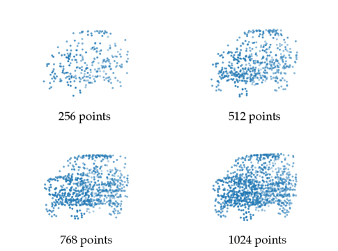
Figure 2: Random sampling of a point cloud of 2,048 points into simplified models of (a) 256 points, (b) 512 points, (c) 768 points and (d) 1,024 points. They are called the random dropout point (DP) models and used as the input to the PointHop system.

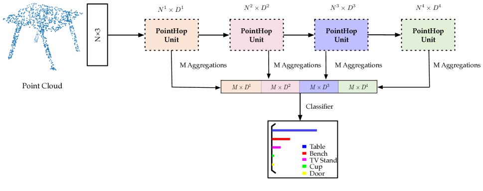
Figure 3: An overview of the PointHop method. The input point cloud has $N$ points with 3 coordinates $(x,y,z)$. It is fed into multiple PointHop units in cascade and their outputs are aggregated by $M$ different schemes to derive features. All features are cascaded for object classification.

A point cloud of $N$ points is defined as ${\bf P}=\{{\bf p}_{1},\cdots,{\bf p}_{N}\}$, where ${\bf p}_{n}\in\mathbb{R}^{3}$, $n=1,\cdots,N$. There are two distinct properties of the point cloud data:

• unordered data in the 3D space
  Being different from images where pixels are defined in a regular 2D grid, a point cloud contains a set of points in the 3D space without a specific order.

• disturbance in scanned points
  For the same 3D object, Different point sets can be acquired with uncertain position disturbance because of different scanning methods applied to the surface of the same object or at different times using the same scanning method.

An overview of the proposed PointHop method is shown in Fig. 3. It takes point cloud, ${\bf P}$, as the input and outputs the corresponding class label. It consists of two stages: 1) local-to-global attribute building through multi-hop information exchange, and 2) classification and ensembles. They will be elaborated in Secs. III-A and III-B, respectively.

III-A Local-to-Global Attribute Building

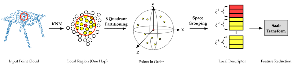
Figure 4: Illustration of the PointHop Unit. The red point is the center point while the yellow points represent its $K$ nearest neighbor points.

In this subsection, we examine the evolution of attributes of a point in ${\bf P}$. Initially, the attributes of a point are its 3D coordinates. Then, we use the attributes of a point and its neighboring points within one-hop distance to build new attributes. Since the new attributes take the relationship between multiple points into account, the dimension of attributes grow. To control the rapid growth of the dimension, we apply the Saab transform for dimension reduction. All these operations are conducted inside a processing unit called the PointHop unit.

The PointHop unit is shown in Fig. 4. It consists of two modules:

1. Constructing a local descriptor with attributes of one-hop neighbors
   The construction takes issues of unordered 3D data and disturbance of scanned points into account to ensure that the local descriptor is robust. The attributes of a point evolve from a low dimensional vector into a high dimensional one through this module.

2. Using the Saab transform to reduce the dimension of the local descriptor
   The Saab transform is used to reduce the dimension of the expanded attributes so that the dimension grows at a slower rate.

For each point in ${\bf P}$, ${\bf p}_{c}=(x_{c},y_{c},z_{c})$, we search its $K$ nearest neighbor points in ${\bf P}$, including itself, where the distance is measured by the Euclidean norm. They form a local region:

$$KNN({\bf p}_{c})=\{{\bf p}_{c1},\cdots,{\bf p}_{cK}\},\quad{\bf p}_{c1},\cdots,{\bf p}_{cK}\in{\bf P}.$$ (1)

For each local region centered at ${\bf p}_{c}$, we treat ${\bf p}_{c}$ as a new origin and partition it into eight quadrants $\xi^{j}$, $j=1,\cdots,8$ based on the value of each coordinate (i.e., greater or less than that of ${\bf p}_{c}$).

We compute the centroid of attributes of points at each quadrant via

$${\bf a}_{c}^{j}=\frac{1}{K_{j}}\sum_{i=1}^{K_{j}}t_{ci}^{j}{{\bf a}_{ci}},\quad,j=1,\cdots,8,$$ (2)

where ${\bf a}_{ci}$ is the attribute vector of point ${\bf p}_{ci}$ and

$$t_{ci}^{j}=\left\{\begin{array}[]{rcl}1,&{x_{ci}\in\xi^{j}},\\ 0,&{x_{ci}\notin\xi^{j}},\end{array}\right.$$ (3)

is the coefficient to indicate whether point $x_{ci}$ is in quadrant $\xi^{j}$ and $K_{j}$ is the number of KNN points in quadrant $\xi^{j}$. Finally, all centroids of attributes ${\bf a}_{c}^{j}$, $j=1,\cdots,8$, are concatenated to form a new descriptor of sampled point ${\bf p}_{c}$:

$${\bf a}_{c}=Concat\{{\bf a}_{c}^{j}\}_{j=1}^{8}.$$ (4)

This descriptor is robust with respect to disturbance in positions of acquired points because of the averaging operation in each quadrant. We use the 3D coordinates, $(x,y,z)$, as the initial attributes of a point. It is called the 0-hop attributes. The dimension of 0-hop attributes is 3. The local descriptor as given in Eq. (4) has a dimension of $3\times 8=24$. We adopt the local descriptor as the new attributes of a point that takes its relationship with its KNN neighbors into account. It is called the 1-hop attributes. Note that the 0-hop attributes can be generalized to $(x,y,z,r,g,b)$ for point clouds with color information $(r,g,b)$ at each point.

If ${\bf p}_{B}$ is a member in $KNN({\bf p}_{A})$, we call that ${\bf p}_{B}$ is a 1-hop neighbor of ${\bf p}_{A}$. If ${\bf p}_{C}$ is a 1-hop neighbor of ${\bf p}_{B}$ and ${\bf p}_{B}$ is a 1-hop neighbor of ${\bf p}_{A}$, we call ${\bf p}_{C}$ is a 2-hop neighbor of ${\bf p}_{A}$ if ${\bf p}_{C}$ is not a 1-hop neighbor of ${\bf p}_{A}$. The dimension of the attribute vector of each point grows from 3 to 24 due to the change of local descriptors from 0-hop to 1-hop. We can build another local descriptor based on the 1-hop attributes of each point. The descriptor defines the 2-hop attributes of dimension $24\times 8=192$. The $n$-hop attributes characterize the relationship of a point with its $m$-hop neighbors, $m\leq n$.

As $n$ becomes larger, the $n$-hop attributes offer a larger coverage of points in a point cloud model, which is analogous to a larger receptive field in deeper layers of CNNs. Yet, the dimension growing rate is fast. It is desired to reduce the dimension of the $n$-hop attribute vector first before reaching out to neighbors of the $(n+1)$-hop. The Saab transform [27] is used to reduce the attribute dimension of each point. A brief review of the Saab transform is given in the Appendix.

Each PointHop unit has one-stage Saab transform. For $L$ PointHop units in cascade, we need $L$-stage Saab transforms. We set $L=4$ in the experiments. Each Saab transform contains three steps: 1) DC/AC separation, 2) PCA and 3) bias addition. The number of AC Saab filters is determined by the energy plot of PCA coefficients as shown in Fig. 5. We choose the knee location of the curve as indicated by the red point in each subfigure.

The system diagram of the proposed PointHop method is shown in Fig. 3. It consists of multiple PointHop units. Four PointHop units are shown in the figure. For the $i$th PointHop unit output, we use $N^{i}\times D^{i}$ to characterize its two parameters; namely, it has $N^{i}$ points and each of them has $D^{i}$ attributes.

For the $i$th PointHop unit, we aggregate (or pool) each individual attribute of $N^{i}$ points into a single feature vector. To enrich the feature set, we consider multiple aggregation/pooling schemes such as the max pooling [16], the mean aggregation, the $l_{1}$-norm aggregation and the $l_{2}$-norm aggregation. Then, we concatenate them to obtain a feature vector of dimension $M\times D^{i}$, where $M$ is the number of attribute aggregation methods, for the $i$th PointHop unit. Finally, we concatenate feature vectors of all PointHop units to form the ultimate feature vector of the whole system.

To reduce computational complexity and speed up the coverage rate, we adopt a spatial sampling scheme between two consecutive PointHop units so that the number of points to be processed is reduced. This is achieved by the farthest point sampling (FPS) scheme [37, 38, 39] since it captures the geometrical structure of a point cloud model better. For a given set of input points, the FPS scheme first selects the point closest to the centroid. Afterwards, it selects the point that has the farthest Euclidean distance to existing points in the selected subset iteratively until the target number is reached. The advantage of the FPS scheme will be illustrated in Sec. IV.

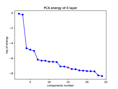
(a) First unit

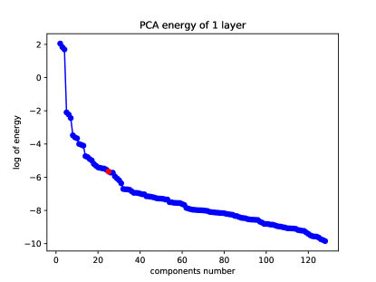
(b) Second unit

(c) Third unit

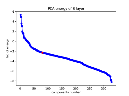
(d) Fourth unit

Figure 5: Determination of the number of Saab filters in each of the PointHop units, where the red dot in each subfigure indicates the selected number of Saab filters.

III-B Classification and Ensembles

Upon obtaining the feature vector, we adopt well known classifiers such as the support vector machine (SVM) and the random forest (RF) classifiers for the classification task. The SVM classifier performs classification by finding gaps that separate different classes. Test samples are then mapped into one of the side of the gap and predicted to be the label of that side. The RF classifier first trains a number of decision trees and each decision tree gives a output. Then, the RF classifier ensembles outputs from all decision trees to give the mean prediction. Both classifiers are mature and easy to use.

Ensemble methods fuse results from multiple weak classifiers to get a more powerful one [40, 41, 26, 42]. Ensembles are adopted in this paper to improve the classification performance furthermore. We consider the following two ensemble strategies.

1. Decision ensemble. Multiple PointHop units are individually used as base classifiers and their decision vectors are concatenated to form a new feature vector for the ensemble classifier.

2. Feature ensemble. Features from multiple PointHop units are cascaded to form the final vector for the classification task.

It is our observation that the second strategy offers better classification accuracy at the cost of a higher complexity if the feature dimension is large. We choose the second strategy for its higher accuracy. With the feature ensemble strategy, it is desired to increase PointHop’s diversity to enrich the feature set. We use the following four schemes to achieve this goal. First, we augment the input data by rotating it with a certain degree. Second, we change the number of Saab filters in each PointHop unit. Third, we change the $K$ value in the KNN scheme. Fourth, we vary the numbers of points in PointHop units.

IV Experimental Results

Feature used

FPS

Pooling

Classifier

Dimension Reduction

Accuracy (%)

All stages

Last stage

Yes

No

Max

Mean

$l_{1}$

$l_{2}$

SVM

Random Forest

PCA

Saab

✓

✓

✓

✓

✓

77.5

✓

✓

✓

✓

✓

77.4

✓

✓

✓

✓

✓

79.6

✓

✓

✓

✓

✓

79.9

✓

✓

✓

✓

✓

78.8

✓

✓

✓

✓

✓

80.2

✓

✓

✓

✓

✓

84.5 (default)

✓

✓

✓

✓

✓

84.8

✓

✓

✓

✓

✓

85.6

✓

✓

✓

✓

✓

✓

85.3

✓

✓

✓

✓

✓

✓

85.7

✓

✓

✓

✓

✓

✓

85.1

✓

✓

✓

✓

✓

✓

✓

✓

86.1

✓

✓

✓

✓

✓

✓

✓

✓

85.6

TABLE I: Results of ablation study with 256 sampled points as the input to the PointHop system.

We conduct experiments on a popular 3D object classification dataset called ModelNet40 [43]. The dataset contains 40 categories of CAD models of objects such as airplanes, chairs, benches, cups, etc. Each initial point cloud has 2,048 points and each point has three Cartesian coordinates. There are 9,843 training samples and 2,468 testing samples.

We adopt the following default setting in our experiments.

• The number of sampled points into the first PointHop unit: 256 points.

• The sampling method from the input point cloud model to that as the input to the first PointHop unit: random sampling.

• The number of $K$ in the KNN: $K=64$.

• The number of PointHop units in cascade: 4.

• The number of Saab AC filters in the $i$th PointHop unit: 15 ($i=1$), 25 ($i=2$), 40 ($i=3$) and 80 ($i=4$).

• The sampling method between PointHop units: Farthest Point Sampling (FPS).

• The number of sampled points in the 2nd, 3rd and 4th PointHop units: 128, 128 and 64.

• The aggregation method: mean pooling.

• The classifier: the random forest classifier.

• Ensembles: No.

This section is organized as follows. First, we conduct an ablation study on an individual PointHop unit and show its robustness against the sampling density variation in Sec. IV-A. Next, we provide results for various ensemble methods in Sec. IV-B. Then, we compare the performance of the proposed PointHop method and other state-of-the-art methods in terms of accuracy and efficiency in Sec. IV-C. After that, we show activation maps of four layers in Sec. IV-D. Finally, we analyze hard samples in Sec. IV-E.

IV-A Ablation Study on PointHop Unit

We show classification accuracy values under various parameter settings in Table I. We see from the table that it is desired to use features from all stages, the FPS between PointHop units, ensembles of all pooling schemes, the random forest classifier and the Saab transform. As shown in the last row, we can reach a classification accuracy of 86.1% with randomly selected 256 points as the input to the PointHop system. The whole training time is 5 minutes only. The FPS not only contributes to higher accuracy but also reduces the computation time dramatically since it can enlarge the receptive field in a faster rate. The RF classifier has a higher accuracy than the SVM classifier. Besides, it is much faster.

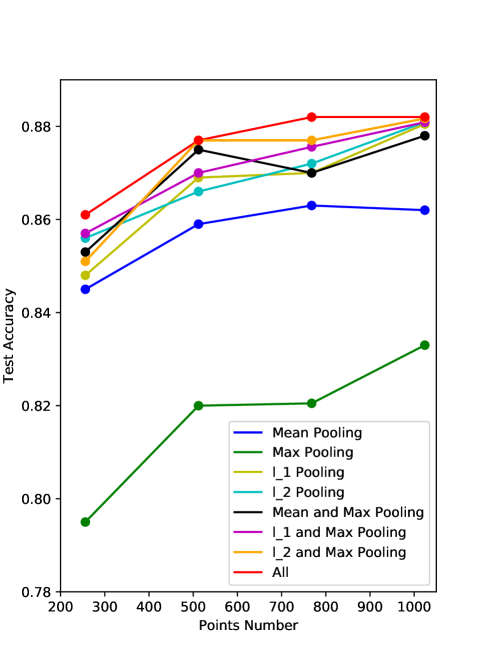
Figure 6: The classification accuracy as a function of the sampled point number of the input model to the PointHop system as well as different pooling methods.

	Setting 1	Setting 2	Setting 3	Setting 4	Setting 5	Ensemble accuracy (%)
HP-A	0°	45°	90°	135°	180°	88.0	88.0
HP-B	(15, 25, 40, 80)	(15, 25, 35, 50)	(18, 30, 50, 90)	(20, 40, 60, 100)	(20, 40, 70, 120)	87.0
HP-C	(64, 64, 64, 64)	(32, 32, 32, 32)	(32, 32, 64, 64)	(96, 96, 96, 96)	(128, 128, 128, 128)	87.8
HP-D	(512, 128, 128, 64)	(512, 256, 128, 64)	(512, 256, 256, 128)	(512, 256, 256, 256)	(512, 128, 128, 128)	86.8

TABLE II: Ensembles of five PointHops with changed hyper-parameter settings and their corresponding classification accuracies.

We study the classification accuracy as a function of the sampled number of all point cloud models as well as different pooling methods in Fig. 6, where the x-axis shows the number of sampled points which is the same in training and testing. Corresponding to Fig. 2, we consider the following four settings: 256 points, 512 points, 768 points and 1,024 points. Different color curves are obtained by different pooling schemes. We compare eight cases: four individual ones, three ensembles of two, and one ensemble of all four. We see that the maximum pooling and the mean pooling give the worst performance. Their ensemble does not perform well, either. The performance gap is small for the remaining five schemes as the point number is 1,024. The ensemble of all pooling schemes given the best results in all four cases. The highest accuracy is 88.2% when we use 768 or 1,024 points with the ensemble of all four pooling schemes.

IV-B Ensembles of PointHop Systems

Under the default setting, we consider ensemble five PointHops with changed hyper-parameters (HP) to increase its diversity. They are summarized in Table II. The hyper parameters of concern include the following four.

• HP-A. We augment each point cloud model by rotating it with 45°four times.

• HP-B. We use different numbers of AC filters in the PointHop units.

• HP-C. We adopt different $K$ values in the KNN query in the PointHop units.

• HP-D. We take point cloud models of different point numbers as the input to the PointHop units in four stages.

For HP-B, HP-C and HP-D, the four numbers in the table correspond to those in the first, second, third and fourth PointHop units, respectively. To get ensemble results of HP-A, we keep HP-B, HP-C and HP-D the same (say, Setting 1). The same procedure applies in getting the ensemble results of HP-B, HP-C and HP-D. Furthermore, we can derive ensemble results of all cases as shown in the last column. We see from the table that the most simple and effective ensemble result is achieved by rotating point clouds, where we can reach the test accuracy of 88%. Thus, we focus on this ensemble method only in later experiments.

IV-C Comparison with State-of-the-Art Methods

We first compare the classification accuracy of the proposed PointHop system with those of several state-of-the-art methods such as PointNet [16], PointNet++ [17], PointCNN [34] and DGCNN [18] in Table III. All of these works (including ours) are based on the model of 1,024 points. The column of “average accuracy” means the average of per-class classification accuracy while the column of “overall accuracy” shows the best result obtained. Our PointHop baseline containing a single model without any ensembles can achieve 88.65% overall accuracy. With ensemble, the overall accuracy is increased to 89.1%. The performance of PointHop is worse than that of PointNet [34] and DGCNN [18] by 0.1% and 3.1%, respectively. On the other hand, our PointHop method performs better than other unsupervised methods such as LFD-GAN [44] and FoldingNet [45].

Method	Feature extraction	Average accuracy (%)	Overall accuracy (%)
PointNet [16]	Supervised	86.2	89.2
PointNet++ [17]		-	90.7
PointCNN [34]		88.1	92.2
DGCNN [18]		90.2	92.2
PointNet baseline (Handcraft, MLP)	Unsupervised	72.6	77.4
LFD-GAN [44]		-	85.7
FoldingNet [45]		-	88.4
PointHop (baseline)		83.3	88.65
PointHop		84.4	89.1

TABLE III: Comparison of classification accuracy on ModelNet40, where the proposed PointHop system achieves 89.1% test accuracy, which is 0.1% less than PointNet [16] and 3.1% less than DGCNN [18].

Next, we compare the time complexity in Table IV. As shown in the table, the training time of the PointHop system is significantly lower than deep-learning-based methods. It takes 5 minutes and 20 minutes in training a PointHop baseline of 256-point and 1,024-point cloud models, respectively, with CPU. Our CPU is Intel(R) Xeon(R) CPU E5-2620 v3 at 2.40GHz. In contrast, PointNet [16] takes more than 5 hours in training using one GTX1080 GPU. Furthermore, we compare the inference time in the test stage. PointNet++ demands 163.2ms in classifying a test sample of 1024 points while our PointHop method only needs 108.4ms. The most time consuming module in the PointHop system is the KNN query that compares the distance between points. It is possible to lower training/testing time even more by speeding up this module.

Method	Total training time	Inference time (ms)	Device
PointNet (1,024 points)	$\sim$ 5 hours	25.3	GPU
PointNet++ (1,024 points)	-	163.2	GPU
PointHop (256 points)	$\sim$ 5 minutes	103	CPU
PointHop (1,024 points)	$\sim$ 20 minutes	108.4	CPU

TABLE IV: Comparison of time complexity between PointNet/PointNet++ and PointHop.

In Fig. 7, we examine the robustness of classification performance with respect to models of four point numbers, i.e., 256, 512, 768 and 1,024. For the first scenario, the numbers in training and testing are the same. It is indicated by DP in the legend. The PointHop method and the PointNet vanilla are shown in violet and yellow lines. The PointHop method with DP is more robust than PointNet vanilla with DP. For the second scenario, we train each method based on 1,024-point models and, then, apply the trained model to point clouds of the same or fewer point numbers in the test. For the latter, there is a point cloud model mismatch between training and testing. We see that the PointHop method is more robust than PointNet++ (SSG) in the mismatched condition. The PointHop method also outperforms DGCNN in the mismatched condition of the 256-point models.

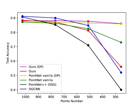
Figure 7: Robustness to sampling density variation: comparison of test accuracy as a function of sampled point numbers of different methods.

IV-D Feature Visualization

The learned features of the first-stage PointHop Unit are visualized in Fig. 8 for six highly varying point cloud models. We show the responses of different channels that are normalized into $[0,1]$ (or from blue to red in color). We see that many common patterns are learned such as corners of tents/lamps and plans of airplanes/beds. The learned features comprise powerful and informative description in the 3D geometric space.

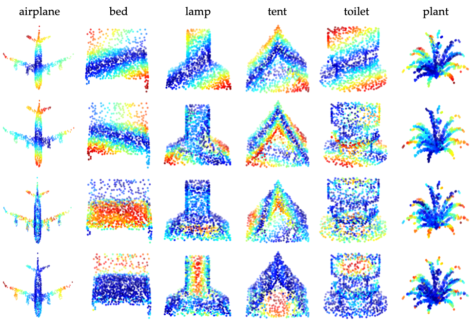
Figure 8: Visualization of learned features in the first-stage PointHop unit.

IV-E Error Analysis

The average accuracy of the PointHop method is worse than PointNet [16] by 1.8%. To provide more insights, we show per-class accuracy on ModelNet40 in Table V. We see that PointHop achieves equal or higher accuracy in 18 classes. On the other hand, it has low accuracy in several classes, including flower-pot (10%), cup (55%), radio (65%) and sink (60%). Among them, the flower pot is the most challenging one.

Network	airplane	bathtub	bed	bench	bookshelf	bottle	bowl	car	chair	cone
PointNet	100.0	80.0	94.0	75.0	93.0	94.0	100.0	97.9	96.0	100.0
PointHop	100.0	94.0	99.0	70.0	96.0	95.0	95.0	97.0	100.0	90.0
	cup	curtain	desk	door	dresser	flower pot	glass box	guitar	keyboard	lamp
PointNet	70.0	90.0	79.0	95.0	65.1	30.0	94.0	100.0	100.0	90.0
PointHop	55.0	85.0	90.7	90.0	83.7	10.0	95.0	99.0	95.0	75.0
	laptop	mantel	monitor	night stand	person	piano	plant	radio	range hood	sink
PointNet	100.0	96.0	95.0	82.6	85.0	88.8	73.0	70.0	91.0	80.0
PointHop	100.0	91.0	98.0	79.1	80.0	82.0	76.0	65.0	91.0	60.0
	sofa	stairs	stool	table	tent	toilet	tv stand	vase	wardrobe	xbox
PointNet	96.0	85.0	90.0	88.0	95.0	99.0	87.0	78.8	60.0	70.0
PointHop	96.0	75.0	85.0	82.0	95.0	97.0	82.0	84.0	70.0	75.0

TABLE V: Comparison of per-class classification accuracy on the ModelNet40.

We conduct error analysis on two object classes, “flower pot” and “cup”, in Figs. 9 (a) and (b), respectively. The total test number of the flower pot class is 20. Eleven, six and one of them are misclassified to the plant, the vase and the lamp classes, respectively. There are only two correct classification cases. We show all point clouds of the flower pot class in Fig. 9 (a). Only the first point cloud has a unique flower pot shape while others have both the flower pot and the plant or are similar to the vase in shape. As to the cup class classification, six are misclassified to the vase class, one misclassified to the bowl class and another one misclassified to the lamp class. There are twelve correct classification results. The errors are caused by shape/functional similarity. To overcome the challenge, we may need to supplement the data-driven approach with the rule-based approach to improve the classification performance furthermore. For example, the height-to-radius ratio of a flower pot is smaller than that of a vase. Also, if the object has a holder, it is more likely to be a cup rather than a vase.

(a) flower pot test samples

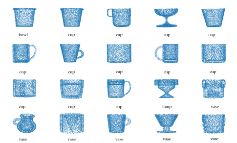
(b) cup test samples

Figure 9: The label under each point cloud is its predicted class. Many flower pots are misclassified to the plant and the vase classes. Also, quite a few cups are misclassified to the vase class.

V Conclusion

An explainable machine learning method called the PointHop method was proposed for point cloud classification in this work. It builds attributes of higher dimensions at each sampled point through iterative one-hop information exchange. This is analogous to a larger receptive field in deeper convolutional layers in CNNs. The problem of unordered point cloud data was addressed using a novel space partitioning procedure. Furthermore, we used the Saab transform to reduce the attribute dimension in each PointHop unit. In the classification stage, we fed the feature vector to a classifier and explored ensemble methods to improve the classification performance. It was shown by experimental results that the training complexity of the PointHop method is significantly lower than that of state-of-the-art deep-learning-based methods with comparable classification performance. We conducted error analysis on hard object classes and pointed out a future research direction for further performance improvement by considering data-driven and rule-based approaches jointly.

Appendix: Saab Transform

The principal component analysis (PCA) is a commonly used dimension reduction technique. The Saab transform uses a specific way to conduct multi-stage PCAs. For an input ${\bf v}=(v_{0},v_{1},\cdots,v_{N-1})^{T}$ of dimension $N$, the one-stage Saab transform can be written as

$$y_{k}=\sum_{n=0}^{N}a_{k,n}v_{n}+b_{k}={{\bf a}^{T}_{k}}{\bf v}+b_{k},\quad k=0,\cdots,K-1$$ (5)

where $y_{k}$ is the $k$th Saab coefficient, ${\bf a}_{k}=(a_{k,0},a_{k,1},\cdots,a_{k,N-1})^{T}$ is the weight vector and $b_{k}$ is the bias term for the $k$th Saab filter. The Saab transform has a particular rule in choosing filter weight ${\bf a}_{k}$ and bias term $b_{k}$.

Let us focus on filter weights first. When $k=0$, the filter is called the DC (direct current) filter, and its filter weight is

$${\bf a}_{0}={\frac{1}{\sqrt{N}}(1,\cdots,1)^{T}}.$$

By projecting input ${\bf v}$ to the DC filter, we get its DC component ${\bf v}_{DC}={\frac{1}{\sqrt{N}}{\sum_{n=0}^{N}}v_{n}}$, which is nothing but the local mean of the input. We can derive the AC component of the input via

$${\bf v}_{AC}={\bf v}-{\bf v}_{DC}.$$

When $k>0$, the filters are called the AC (alternating current) filters. To derive AC filters, we conduct PCA on AC components, ${\bf v}_{AC}$, and choose its first $(K-1)$ principle components as the AC filters ${\bf a}_{k},k=1,\cdots,K-1$. Finally, the DC filter and $K-1$ AC filters form the set of Saab filters.

Next, we discuss the choice of the bias term, $b_{k}$, of the $k$th filter. In CNNs, there is an activation function at the output of each convolutional operation such as the ReLU (Rectified Linear Unit) and the sigmoid. In the Saab transform, we demand that all bias terms are the same so that they contribute to the DC term in the next stage. Besides, we choose the bias large enough to guarantee that the response $y_{k}$ is always non-negative before the nonlinear activation operation. Thus, nonlinear activation plays no role and can be removed. It is shown in [27] that $b_{k}$ can be selected using the following rule:

$$b_{k}=\mbox{constant}\geq{\max\limits_{\bf v}{\left\|{\bf v}\right\|}},\quad k=0,\cdots,N-1.$$

Pixels in images have a decaying correlation structure. The correlation between local pixels is stronger and the correlation becomes weaker as their distance becomes larger. To exploit this property, we conduct the first-stage PCA in a local window for dimension reduction to get a local spectral vector. It will result in a joint spatial-spectral cuboid where the spatial dimension denotes the spatial location of the local window and the spectral dimension provides the spectral components of the corresponding window. Then, we can perform the second-stage PCA on the joint spatial-spectral cuboid. The multi-stage PCA is better than the single-stage PCA since it handles decaying spatial correlations in multiple spatial resolutions rather than in a single spatial resolution.

Min Zhang received her B.E. degree from the School of Science, Nanjing University of Science and Technology, Nanjing, China and her M.S. degree from the Viterbi School of Engineering, University of Southern California, Los Angeles, US, in 2017 and 2019, respectively. She is currently working toward the Ph.D. degree from University of Southern California. Her research interests include pattern recognition and machine learning, image and video processing, object segmentation, detection and tracking.

Haoxuan You received his Bachelor of Engineering degree in Electronics Information Engineering from Xidian University, Xian, China in 2018. He is currently pursuing Ph.D. degree in Computer Science from Columbia University, New York, USA. His research interests lie in computer vision including 3D object recognition, 3D object detection, multimodal learning and machine learning especially hypergraph learning.

Pranav Kadam received the Bachelor of Engineering degree in Electronics and Telecommunication from Savitribai Phule Pune University, Pune, India in 2018. He is currently pursuing M.S. degree in Electrical Engineering with specialization in signal and image processing from University of Southern California, Los Angeles, USA. His research interests include computer vision and applications of machine learning and deep learning techniques in image and video analysis.

Shan Liu is a Distinguished Scientist and General Manager at Tencent where she heads the Tencent Media Lab. Prior to joining Tencent she was the Chief Scientist and Head of America Media Lab at Futurewei Technologies. She was formerly Director of Multimedia Technology Division at MediaTek USA. She was also formerly with MERL, Sony and IBM. Dr. Liu is the inventor of more than 200 US and global patent applications and the author of more than 50 journal and conference articles. She actively contributes to international standards such as VVC, H.265/HEVC, DASH, OMAF, and served as co-Editor of H.265/HEVC v4 and VVC. Dr. Liu obtained her B.Eng. degree in Electronics Engineering from Tsinghua University, Beijing, China and M.S. and Ph.D. degrees in Electrical Engineering from University of Southern California, Los Angeles, USA.

C.-C. Jay Kuo (F’99) received the B.S. degree in electrical engineering from the National Taiwan University, Taipei, Taiwan, in 1980, and the M.S. and Ph.D. degrees in electrical engineering from the Massachusetts Institute of Technology, Cambridge, in 1985 and 1987, respectively. He is currently the Director of the Multimedia Communications Laboratory and a Distinguished Professor of electrical engineering and computer science at the University of Southern California, Los Angeles. His research interests include digital image/video analysis and modeling, multimedia data compression, communication and networking, and biological signal/image processing. He is the coauthor of about 280 journal papers, 940 conference papers and 14 books. Dr. Kuo is a Fellow of the American Association for the Advancement of Science (AAAS) and The International Society for Optical Engineers (SPIE).

References

- [1] C. R. Qi, H. Su, M. Nießner, A. Dai, M. Yan, and L. J. Guibas, “Volumetric and multi-view cnns for object classification on 3d data,” in Proceedings of the IEEE conference on computer vision and pattern recognition, 2016, pp. 5648–5656.
- [2] H. You, Y. Feng, R. Ji, and Y. Gao, “Pvnet: A joint convolutional network of point cloud and multi-view for 3d shape recognition,” in 2018 ACM Multimedia Conference on Multimedia Conference. ACM, 2018, pp. 1310–1318.
- [3] G. Riegler, A. Osman Ulusoy, and A. Geiger, “Octnet: Learning deep 3d representations at high resolutions,” in Proceedings of the IEEE Conference on Computer Vision and Pattern Recognition, 2017, pp. 3577–3586.
- [4] P. Papadakis, I. Pratikakis, T. Theoharis, and S. Perantonis, “Panorama: A 3d shape descriptor based on panoramic views for unsupervised 3d object retrieval,” International Journal of Computer Vision, vol. 89, no. 2-3, pp. 177–192, 2010.
- [5] D. Maturana and S. Scherer, “Voxnet: A 3d convolutional neural network for real-time object recognition,” in 2015 IEEE/RSJ International Conference on Intelligent Robots and Systems (IROS). IEEE, 2015, pp. 922–928.
- [6] A. Brock, T. Lim, J. M. Ritchie, and N. Weston, “Generative and discriminative voxel modeling with convolutional neural networks,” arXiv preprint arXiv:1608.04236, 2016.
- [7] H. Su, S. Maji, E. Kalogerakis, and E. Learned-Miller, “Multi-view convolutional neural networks for 3d shape recognition,” in Proceedings of the IEEE international conference on computer vision, 2015, pp. 945–953.
- [8] Y. Feng, Z. Zhang, X. Zhao, R. Ji, and Y. Gao, “Gvcnn: Group-view convolutional neural networks for 3d shape recognition,” in Proceedings of the IEEE Conference on Computer Vision and Pattern Recognition, 2018, pp. 264–272.
- [9] Y. Feng, Y. Feng, H. You, X. Zhao, and Y. Gao, “Meshnet: Mesh neural network for 3d shape representation,” arXiv preprint arXiv:1811.11424, 2018.
- [10] Z. Zhang, H. Lin, X. Zhao, R. Ji, and Y. Gao, “Inductive multi-hypergraph learning and its application on view-based 3d object classification,” IEEE Transactions on Image Processing, vol. 27, no. 12, pp. 5957–5968, 2018.
- [11] L. Landrieu and M. Simonovsky, “Large-scale point cloud semantic segmentation with superpoint graphs,” in Proceedings of the IEEE Conference on Computer Vision and Pattern Recognition, 2018, pp. 4558–4567.
- [12] M. Angelina Uy and G. Hee Lee, “Pointnetvlad: Deep point cloud based retrieval for large-scale place recognition,” in Proceedings of the IEEE Conference on Computer Vision and Pattern Recognition, 2018, pp. 4470–4479.
- [13] B. Yang, M. Liang, and R. Urtasun, “Hdnet: Exploiting hd maps for 3d object detection,” in Conference on Robot Learning, 2018, pp. 146–155.
- [14] B. Yang, W. Luo, and R. Urtasun, “Pixor: Real-time 3d object detection from point clouds,” in Proceedings of the IEEE Conference on Computer Vision and Pattern Recognition, 2018, pp. 7652–7660.
- [15] A. H. Lang, S. Vora, H. Caesar, L. Zhou, J. Yang, and O. Beijbom, “Pointpillars: Fast encoders for object detection from point clouds,” in Proceedings of the IEEE Conference on Computer Vision and Pattern Recognition, 2019, pp. 12 697–12 705.
- [16] C. R. Qi, H. Su, K. Mo, and L. J. Guibas, “Pointnet: Deep learning on point sets for 3d classification and segmentation,” in Proceedings of the IEEE Conference on Computer Vision and Pattern Recognition, 2017, pp. 652–660.
- [17] C. R. Qi, L. Yi, H. Su, and L. J. Guibas, “Pointnet++: Deep hierarchical feature learning on point sets in a metric space,” in Advances in Neural Information Processing Systems, 2017, pp. 5099–5108.
- [18] Y. Wang, Y. Sun, Z. Liu, S. E. Sarma, M. M. Bronstein, and J. M. Solomon, “Dynamic graph cnn for learning on point clouds,” arXiv preprint arXiv:1801.07829, 2018.
- [19] Y. Shen, C. Feng, Y. Yang, and D. Tian, “Mining point cloud local structures by kernel correlation and graph pooling,” in Proceedings of the IEEE conference on computer vision and pattern recognition, 2018, pp. 4548–4557.
- [20] C. Cortes and V. Vapnik, “Support-vector networks,” Machine learning, vol. 20, no. 3, pp. 273–297, 1995.
- [21] L. Breiman, “Random forests,” Machine learning, vol. 45, no. 1, pp. 5–32, 2001.
- [22] C.-C. J. Kuo, “Understanding convolutional neural networks with a mathematical model,” Journal of Visual Communication and Image Representation, vol. 41, pp. 406–413, 2016.
- [23] Y. Chen, Z. Xu, S. Cai, Y. Lang, and C.-C. J. Kuo, “A saak transform approach to efficient, scalable and robust handwritten digits recognition,” in 2018 Picture Coding Symposium (PCS). IEEE, 2018, pp. 174–178.
- [24] C.-C. J. Kuo, “The cnn as a guided multilayer recos transform [lecture notes],” IEEE signal processing magazine, vol. 34, no. 3, pp. 81–89, 2017.
- [25] C.-C. J. Kuo and Y. Chen, “On data-driven saak transform,” Journal of Visual Communication and Image Representation, vol. 50, pp. 237–246, 2018.
- [26] Y. Chen, Y. Yang, W. Wang, and C.-C. J. Kuo, “Ensembles of feedforward-designed convolutional neural networks,” arXiv preprint arXiv:1901.02154, 2019.
- [27] C.-C. J. Kuo, M. Zhang, S. Li, J. Duan, and Y. Chen, “Interpretable convolutional neural networks via feedforward design,” Journal of Visual Communication and Image Representation, 2019.
- [28] S. Wold, K. Esbensen, and P. Geladi, “Principal component analysis,” Chemometrics and intelligent laboratory systems, vol. 2, no. 1-3, pp. 37–52, 1987.
- [29] J. Sun, M. Ovsjanikov, and L. Guibas, “A concise and provably informative multi-scale signature based on heat diffusion,” in Computer graphics forum, vol. 28, no. 5. Wiley Online Library, 2009, pp. 1383–1392.
- [30] M. M. Bronstein and I. Kokkinos, “Scale-invariant heat kernel signatures for non-rigid shape recognition,” in 2010 IEEE Computer Society Conference on Computer Vision and Pattern Recognition. IEEE, 2010, pp. 1704–1711.
- [31] M. Aubry, U. Schlickewei, and D. Cremers, “The wave kernel signature: A quantum mechanical approach to shape analysis,” in 2011 IEEE international conference on computer vision workshops (ICCV workshops). IEEE, 2011, pp. 1626–1633.
- [32] R. B. Rusu, N. Blodow, Z. C. Marton, and M. Beetz, “Aligning point cloud views using persistent feature histograms,” in 2008 IEEE/RSJ International Conference on Intelligent Robots and Systems. IEEE, 2008, pp. 3384–3391.
- [33] D.-Y. Chen, X.-P. Tian, Y.-T. Shen, and M. Ouhyoung, “On visual similarity based 3d model retrieval,” in Computer graphics forum, vol. 22, no. 3. Wiley Online Library, 2003, pp. 223–232.
- [34] Y. Li, R. Bu, M. Sun, W. Wu, X. Di, and B. Chen, “Pointcnn: Convolution on x-transformed points,” in Advances in Neural Information Processing Systems, 2018, pp. 820–830.
- [35] C. R. Qi, W. Liu, C. Wu, H. Su, and L. J. Guibas, “Frustum pointnets for 3d object detection from rgb-d data,” in Proceedings of the IEEE Conference on Computer Vision and Pattern Recognition, 2018, pp. 918–927.
- [36] Y. Zhou and O. Tuzel, “Voxelnet: End-to-end learning for point cloud based 3d object detection,” in Proceedings of the IEEE Conference on Computer Vision and Pattern Recognition, 2018, pp. 4490–4499.
- [37] I. Katsavounidis, C.-C. J. Kuo, and Z. Zhang, “A new initialization technique for generalized lloyd iteration,” IEEE Signal processing letters, vol. 1, no. 10, pp. 144–146, 1994.
- [38] Y. Eldar, M. Lindenbaum, M. Porat, and Y. Y. Zeevi, “The farthest point strategy for progressive image sampling,” IEEE Transactions on Image Processing, vol. 6, no. 9, pp. 1305–1315, 1997.
- [39] C. Moenning and N. A. Dodgson, “Fast marching farthest point sampling,” University of Cambridge, Computer Laboratory, Tech. Rep., 2003.
- [40] T. G. Dietterich, “Ensemble methods in machine learning,” in International workshop on multiple classifier systems. Springer, 2000, pp. 1–15.
- [41] L. Rokach, “Ensemble-based classifiers,” Artificial Intelligence Review, vol. 33, no. 1-2, pp. 1–39, 2010.
- [42] C. Zhang and Y. Ma, Ensemble machine learning: methods and applications. Springer, 2012.
- [43] Z. Wu, S. Song, A. Khosla, F. Yu, L. Zhang, X. Tang, and J. Xiao, “3d shapenets: A deep representation for volumetric shapes,” in Proceedings of the IEEE conference on computer vision and pattern recognition, 2015, pp. 1912–1920.
- [44] P. Achlioptas, O. Diamanti, I. Mitliagkas, and L. Guibas, “Representation learning and adversarial generation of 3d point clouds,” arXiv preprint arXiv:1707.02392, vol. 2, no. 3, p. 4, 2017.
- [45] Y. Yang, C. Feng, Y. Shen, and D. Tian, “Foldingnet: Point cloud auto-encoder via deep grid deformation,” in Proceedings of the IEEE Conference on Computer Vision and Pattern Recognition, 2018, pp. 206–215.