Alignment between Satellite and Central Galaxies in the Eagle Simulation: Dependence on the Large-Scale Environments

Abstract

The alignment between satellite and central galaxies serves as a proxy for addressing the issue of galaxy formation and evolution and has been investigated abundantly in observations and theoretical works. Most scenarios indicate that the satellites preferentially locate along the major axis of their central galaxy. Recent work shows that the strength of alignment signals depends on large-scale environment in observations. We use the publicly-released data from EAGLE to figure out whether the same effect can be found in the hydrodynamic simulation. We found much stronger environmental dependency of alignment signal in simulation. And we also explore change of alignments to address the formation of this effects.

1 Introduction

The standard $\Lambda$ cold dark matter cosmology suggests a hierarchical scenario of cosmic structure formation. The growth of Gaussian density fluctuations via highly nonlinear and anisotropic gravitational clustering process shape the large scale structure of universe with four distinct environments, i.e. cluster, filament, sheet and void (Jõeveer et al. 1978; Bond et al. 1996). Flowing out of the voids, matter accrete on the sheets, then collapse onto the filaments and finally assemble to form clusters at the intersections of filaments. On smaller scales, dark matter collapses to small halos firstly and then may go through merges with other halos to form larger halo or been captured by larger halos to become their ”sub-halos”, and galaxies are formed in the inner region of these dark matter halos (White & Rees 1978). According to this paradigm, galaxies are not randomly distributed in the universe, but rather show some alignments, i.e. the shape, position , spin etc. tend to have preferential directions (Jing & Suto 2002; Aubert et al. 2004; Bagla & Prasad 2006; Aragón-Calvo et al. 2010; Arieli et al. 2010). Thus, the galaxy alignment could be an indicator for probing the galaxy formation and evolutionary history in the $\Lambda$ CDM universe.

Many observational and theoretical works have confirmed galaxy alignments. Explorations on galaxy alignments in observation started began with the early works Sastry (1968) and Holmberg (1969). The former reported an alignment between satellite galaxies and major axis of central galaxies. But the latter claimed the opposite results that the position vectors of satellite galaxies tend to be perpendicular to the major axis of central galaxies. The disagreement of these two works may partly result from the small survey volume of the galaxy sample, such a defect has been overcome by the emergence of large galaxy surveys, e.g., Sloan Digital Sky Survey (SDSS). Benefited from super-large volume of galaxy sample, studies on central-satellite galaxy alignments has already reached a unified and largely accepted conclusion that the satellites tend to align with the major axis of central galaxy (e.g., Agustsson & Brainerd 2006b; Yang et al. 2006; Brainerd 2005; Agustsson & Brainerd 2010). Following theoretical works by utilizing semi-analytical models, both N-body simulations and hydrodynamical simulations has confirmed such a trend (Agustsson & Brainerd 2006a; Kang et al. 2007; Libeskind et al. 2005, 2007; Codis et al. 2012, 2015). For a full overview on all kinds of issues about galaxy alignments, in which the central-satellite alignment is just one aspect, readers could refer to Schäfer (2009); Joachimi et al. (2015); Kiessling et al. (2015); Kirk et al. (2015).

The central-satellite alignment comes from the combination of smooth mass accretion and mergers of dark matter halos. The anisotropic collapse of dark matter halo will shape its central galaxy with preferential directions Jing & Suto (2002); Schäfer (2009). As a result, the direction of axes, or angular momentum, of central galaxies will relate with their surrounding structures.(Zhang et al. 2013, 2015) On the other hand, as remnants of accreted halos, merger events can be inferred from the position of satellite galaxies. Thereby the alignment between the position of satellite galaxies and direction of large scale structures was also studied (e.g., Tempel et al. 2015). However, detecting these two processes separately could be tough due to sort of ambiguities in defining the shape and direction of large scale structures from observational data, leading to most work focusing on the central-satellite alignments.

In the different structure type of the cosmic web, e.g., cluster, filament, sheet and void, the central-satellite alignment could be quite different, because of either dark matters collapsing via different directions (Codis et al. 2018), or subhaloes (satellite galaxies) being accreted via different paths dictated by large scale structures Libeskind et al. (2014). Accordingly, the shape of central galaxy and the distribution of satellite galaxies may be influenced by the local structure types. Many works found that the shape of dark matter halo, which should be shapely aligned with its central galaxy, is related with local structures (Hahn et al. 2007; Zhang et al. 2009; Forero-romero et al. 2014). Tempel & Libeskind (2013) found that the minor axes of elliptical galaxies are preferentially perpendicular to hosting filaments but the alignment signal is weak in sheets. And the spin axes of spirals align with host filaments, but there is no alignment signal between the spiral spin and the sheet normal vector. Codis et al. (2018) confirmed the same trend and further revealed an alignment flipping phenomenon from high to low redshifts. Some works like Tempel et al. (2015) confirmed that the angular positions of satellite galaxies tend to align with filaments. A further explanation is provided by Libeskind et al. (2015), in which they claimed that the plane of satellite galaxies’ orbit is well aligned with the collapse direction derived from the shear tensor of environmental velocity fields.

Since the large scale structures have influences on both central galaxies and satellite galaxies, we would expect the alignment between them depending on the local cosmic environments. It would be interesting to examine this issue, and recently Wang et al. (2018) have done such exploration. Wang et al. (2018) found environment dependence of the alignment between satellite and central galaxies in the SDSS DR7 data. Following Wang et al. (2018), we would like to examine whether this dependence exists for simulated galaxies in cosmological hydrodynamical simulation, and to explore the possible explanation for this phenomenon.

The paper is organized as follows: we brief firstly the simulation and the galaxy catalogue, definitions of large-scale structure and alignment angles in Section 2. Then the main results are given in Section 3. Finally, we give discussions and conclusions in Section 4.

2 Data and Methodology

In this work, we use the publicly released data from the Evolution and Assembly of Galaxies and their Environments (EAGLE) simulation (Schaye et al. 2015) , which was run using a modified version of the code GADGET 2 (Springel 2005). The cosmology parameters are $\Omega_{m}=0.307,\Omega_{b}=0.04825,\sigma_{8}=0.8288,n_{s}=0.9611,h=0.6777$. We take advantage of the simulation run labelled of “Ref- L100N1504”, i.e., with a box size of $100\rm Mpc$, particles number of $2\times 1504^{3}$ , and softening length of $2.66\rm kpc$. The mass resolutions of gas and dark matter particles are $1.81\times 10^{6}h^{-1}M_{\odot}$ and $9.70\times 10^{6}h^{-1}M_{\odot}$. Stellar particles have variable mass around $7\times 10^{5}h^{-1}M_{\odot}$. More details about EAGLE simulation can be found in Schaye et al. (2015).

2.1 Galaxies Samples

We use five snapshots (z=0,1,2,3,5) from the simulation for data analysis. The dark matter halos are identified by the standard friends-of-friends (FOF) algorithm (Davis et al. 1985). Dark matter particles within a linking length of $0.2$ times of the mean inter particle separation are assigned to the same dark matter halo. Gas and star particles are assigned to the FoF halo where their nearest dark matter particles reside in. The subhaloes are found by the SUBFIND algorithm (Springel et al. 2001; Dolag et al. 2009). We select central-satellite pairs from the $10000$ most massive dark matter halos. In remaining less massive halos, no satellite galaxies could be found due to the small number of star particles. We further place a constrain on the galaxy sample that only galaxies with more than $100$ star particles are taken for analysis, corresponding to stellar mass of $7\times 10^{7}h^{-1}M_{\odot}$. The number of central-satellite galaxy pairs selected is listed in Table 1.

Table 1: Number of central-satellite pairs selected at different redshifts.

z	0	1	2	3	5
pair number	21693	14566	10740	5914	1168

2.2 Characterize The Large Scale Environment

The structure types in the large scale environment, namely cluster, filament, sheet and void, are defined following the same method applied in Hahn et al. (2007), Forero-Romero et al. (2009) and Zhu & Feng (2017). We calculate the three eigenvalues of the Hessian matrix of the tidal field on specific grids

$$T_{i,j}=\frac{\partial^{2}\phi}{\partial{r_{i}}\partial{r_{j}}}$$ (1)

where $\phi$ is the potential there and $i,j$ go from $1$ to $3$ to cover the $3$ directions. For each grid, we count the numbers of eigenvalues above a certain threshold $\lambda_{t}$. If all three eigenvalues are larger than $\lambda_{t}$, the structure type around that point will be tagged cluster. Similarly, we sort out all particle, each with two, one or none eigenvalues larger than the threshold $\lambda_{t}$ corresponding to filament, sheet and void respectively. In many works $\lambda_{t}$ is set to be $0$ (Hahn et al. 2007). However, some works suggest a larger value of $\lambda_{t}$ (Zhu & Feng 2017; Forero-Romero et al. 2009) to avoid producing smaller volume of voids with $\lambda_{t}=0$ than the theoretical prediction. Visually, a reasonable classification of the large scale structure can be given by setting $\lambda=2.0$. Figure 1 displays the matter distribution(left) and corresponding environments(right) in a slice of simulation at redshift $0$, where cells of different structures are assigned with different colors.

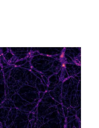
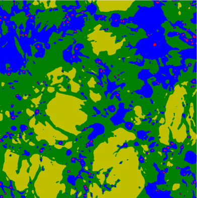
Figure 1: Left figure shows the density field of a slice with volume of $100{\rm Mpc}\times 100{\rm Mpc}\times 60{\rm Kpc}$ at redshift $0$. Right Figure indicate the large scale structure within the same region. Red regions are clusters, greens are filaments, blues are sheets and yellows are voids.

2.3 Characterize The Alignment

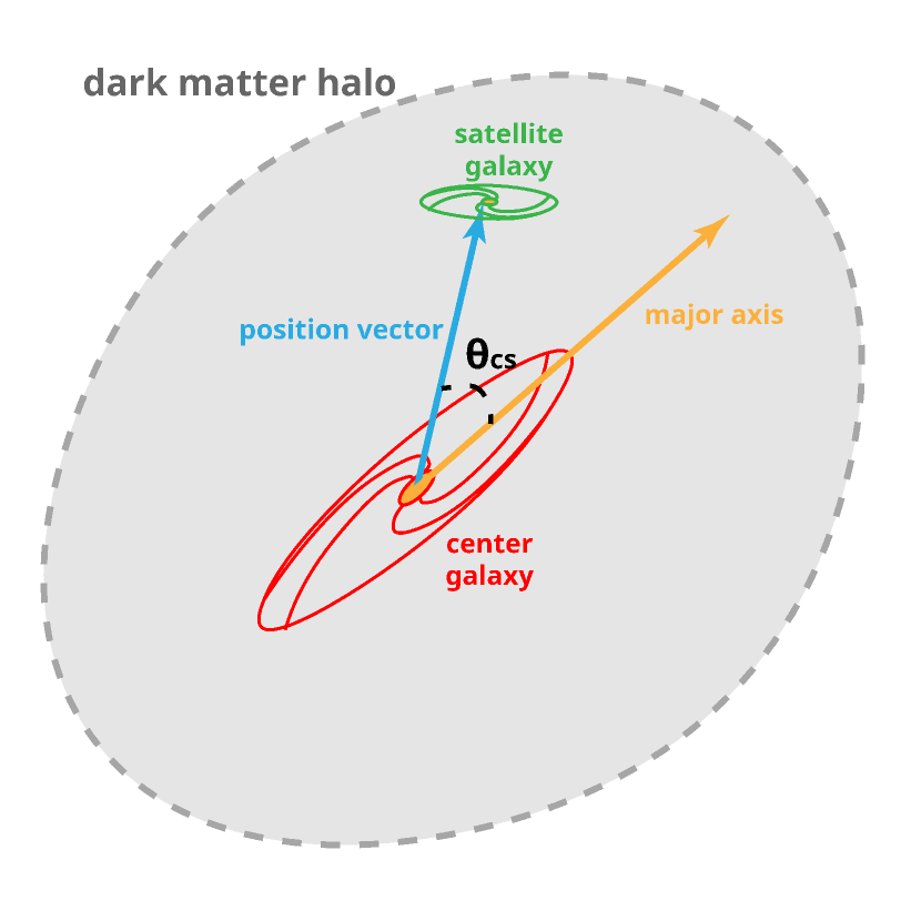
Figure 2: A figure illustrating the central-satellite alignment angle. The red and green ellipse represent the central and satellite galaxies. The yellow vector represents the major axis of center galaxy. The blue vector direct from the center of central galaxy to the center of satellite galaxy. The angular separation between blue and yellow vectors $\theta_{CS}$ is the alignment angle.

In this paper we analyze the alignment angle between the major axis direction of the central galaxy and the position direction of satellites, as illustrated in Figure 2. The red arrow represents the major axis of the central galaxy. The blue arrow represents the direction of the satellite relative to the central of the central galaxy, and $\theta_{CS}$ is the alignment angle. The major axis of the central galaxy is determined by the mass weighted shape matrix whose element is defined as:

$$I_{ij}=\frac{\sum_{k}m_{k}x_{k,i}x_{k,j}}{\sum_{k}m_{k}}$$ (2)

where $m_{k}$ is the mass of the $k\rm th$ star particle in the central galaxy, , $x_{k,i}$ is the coordinate of $k\rm th$ star particle along $i\rm th$ axis ($i$ ranges from $1$ to $3$), and the summation is taken over all the star particles in the central galaxy. Once the shape matrix $I=\{I_{ij},i,j=1,2,3\}$ is obtained, the major axis can be specified by the eigenvector corresponding to the maximum eigenvalue of the shape matrix.

The alignment angle $\theta_{CS}$ ranges from $0^{\circ}$ to $90^{\circ}$, and a relative small value of $\theta<45^{\circ}$ implies preferentially aligned distribution along the major axis of central galaxy. To compare with observations, we project central galaxies and satellites onto a 2-dimensional plane before calculating the alignment angle $\theta_{CS}$. The projection onto the $x-y$ plane can be made simply by setting the $z$ coordinate of all particles to be zero. We also tested projections onto the $x-z$ and $y-z$ plane. No significant differences have been found among the three projecting direction. In the following, results are obtained by projected galaxies on the $x-y$ plane if not specified elsewhere.

3 Results

In this section, we first present the color and mass dependence of central-satellite alignment following the previous works Yang et al. (2006); Wang et al. (2018). Then we check numerically the dependence on various structure types in the cosmic web to test whether we could reproduce Wang et al. (2018)’s results. Finally, we make an attempt to explore the origin of dependency on large scale environment by tracing alignment signal $\theta_{CS}$ through the cosmic time.

3.1 The color and mass dependence of central-satellite alignments

Following Yang et al. (2006) and Wang & Kang (2018), we first check the overall alignment signal. As shown in the first row of Table 2, the mean alignment angle in EAGLE simulation is smaller than Yang et al. (2006) and Wang & Kang (2018), indicating a stronger alignment. According to the previous works e.g. Kang et al. (2007); Faltenbacher et al. (2009), the alignment between subhalo and the major axis of host halo is much stronger than that between satellite galaxies and the major axis of central galaxies. To reproduce the alignment signal inferred from the observations, the misalignment between central galaxy and host halo is necessary inevitably. Wang et al. (2014); Faltenbacher et al. (2009) suggest a misalignment angle around $30^{\circ}$, which has been justified by Dong et al. (2014) using the hydrodynamical cosmological simulation. However, we calculate the misalignment between central galaxy and host halo in the EAGLE’s data, and found that it peaks at about $20^{\circ}$. This could be a reason why the stronger alignment signal has been found in that work. The physics behind such small misalignment might be complex, thus we leave it for future work.

Table 2: Mean alignment angle $\theta_{CS}$ of different (sub-)samples of central-satellites galaxy pairs at redshift $0$ in EAGLE simulation (fourth column), compared with the results in Yang et al. (2006)(second column) and Wang et al. (2018)(third column). Sub samples are divided according to galaxy color. In row $2$ to $3$ only the color of central galaxies is considered. In row $4$ and $5$, we only consider the satellites’ color. In row $6$ to $9$, the sample make constrains on both centrals and satellites. The sample name ’red - blue’ means the galaxy paris have red centrals and blue satellites.

Sample Name	Y06	W18	This Work
all sample	$42.2\pm 0.2^{\circ}$	$42.2\pm 0.06^{\circ}$	$38.1\pm 0.3^{\circ}$
red centrals	$41.5\pm 0.2^{\circ}$	$41.7\pm 0.10^{\circ}$	$38.2\pm 0.3^{\circ}$
blue centrals	$44.5\pm 0.5^{\circ}$	$44.7\pm 0.15^{\circ}$	$38.0\pm 0.7^{\circ}$
red satellites	$41.5\pm 0.3^{\circ}$	$41.5\pm 0.11^{\circ}$	$36.0\pm 0.5^{\circ}$
blue satellites	$43.3\pm 0.3^{\circ}$	$43.2\pm 0.09^{\circ}$	$39.3\pm 0.3^{\circ}$
red - red	$40.8\pm 0.3^{\circ}$	$40.9\pm 0.12^{\circ}$	$36.0\pm 0.5^{\circ}$
red - blue	$42.9\pm 0.3^{\circ}$	$42.6\pm 0.13^{\circ}$	$39.5\pm 0.4^{\circ}$
blue - red	$44.8\pm 0.7^{\circ}$	$45.5\pm 0.31^{\circ}$	$36.6\pm 1.3^{\circ}$
blue - blue	$44.2\pm 0.6^{\circ}$	$44.4\pm 0.20^{\circ}$	$38.4\pm 0.8^{\circ}$

The rest rows of Table 1 show the color dependence of the alignment signal. The color of a galaxy is defined by its magnitude $g-r$. For the probability distribution of $g-r$, there appear two peaks. We use the median value of these two peaks to classify galaxies into the red and blue branches. This method was suggested by Baldry et al. (2004) and has been widely used. In Yang et al. (2006) and Wang & Kang (2018), the red centrals or red satellites have smaller alignment angles. Galaxies in EAGLE are unable to fully reproduce such trends. In our samples, the red satellites align with the centrals’ major axis more strongly, while for the red and blue central galaxies, they have similar alignment signals. However, it is always a challenge to fully recover the alignment dependency on the galaxy color. Our results are quite similar to Dong et al. (2014). Their results also eliminate the differences between blue and red central galaxies. It is basically caused by the fact that relatively more blue central galaxies are produced in the simulation than observation. As displayed in figure 2 and 4 in Trayford et al. (2015), the $g-r$ versus $M_{*}$ or $g-r$ versus $M_{r}$ profile in the EAGLE simulation has similar outer shape and blue peak as GAMA galaxies, but it does not recover the red peak. Thus some central galaxies with the strong alignment are mis-assigned to blue color. Trayford et al. (2015) suggested that the flat slope of red sequence may be attributed to the rapidly decreased stellar metallicity at low mass range, and such decrement may be a resolution issue of the simulation.

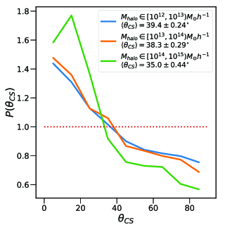
Figure 3: The normalized probability distribution of the alignment angle $\theta_{CS}$. Central-satellite pairs are assigned into $3$ sub samples according to their host halo’s mass, as indicated by the legend. The mean angle for each sub sample is also shown in the legend. The red dotted horizontal line $P=1$ represents a ideal isotropic distribution.

We also check the dependence on the mass of host halo. The probability distribution of the alignment angle $\theta_{CS}$ is shown in Figure 3. The probability distribution is obtain by computing $P(\theta)=N(\theta)/N_{R}(\theta)$. $N(\theta)$ is the number of central-satellite pairs with the alignment angle of $\theta$ in the samples to be studied. $N_{R}(\theta)$ is the number of galaxy pairs with the same $\theta$ in a sample with randomly distributed satellite galaxies. The total number of galaxy pairs of random sample is the same as the simulation sample. Figure 3 shows that the alignment is clearly dependent on the halo mass. Galaxy pairs in the massive halos exhibit stronger alignment. This trends are in agreement with Yang et al. (2006); Kang et al. (2007); Wang et al. (2014); Wang & Kang (2018).

In summary, the EAGLE’s galaxy catalogue reproduces both the mass and color dependence (partly) of alignment in the observations. It also encounters problems like too stronger alignment signal and blue biased central galaxies, but these problems also exist in many other simulations. On the other hand, the overall trend is quite reasonable. Thus the drawback does not border the main part of our work, exploring the environmental effect of large scale structures on the alignment.

3.2 The Environment Influence of the Large Scale Structures

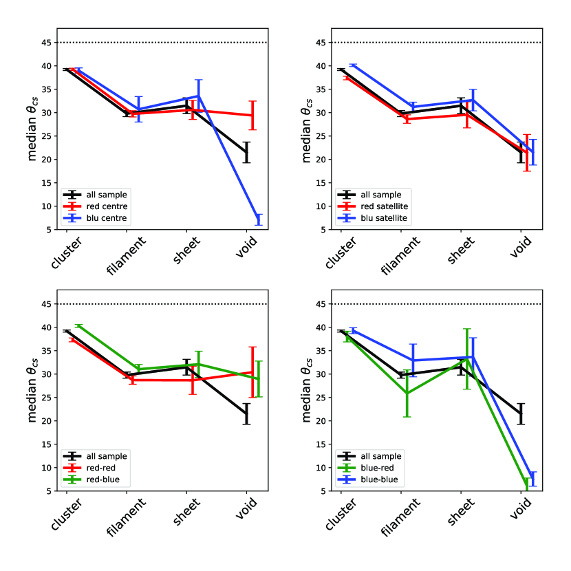
Figure 4: Average alignment angle in different environment at redshift $0$. Galaxy pairs are divided into different catalogues according to the color of central or satellite galaxies. The upper-left panel shows the difference between galaxy pairs with red and blue centrals. The upper-right panel compares the samples with red satellites and blue satellites. The lower left panel shows red centrals - red satellites samples versus red centrals - blue satellite, while the lower right shows blue centrals - red satellites sample versus blue centrals - blue satellites sample. A black solid line indicating the overall trend is shown in all panels. Black dotted line at $\langle\theta\rangle=45^{\circ}$ show the average alignment level of random distribution of satellites. The error bars indicate the Poisson error of mean $\theta_{CS}$. To make the error bars clear, we shift lines a bit horizontally.

Table 3: The mean $\theta_{CS}$ in different environments. Sub-samples are the same as Table 2. For short ”satellite galaxy” is written as ”sat”.

	Cluster	Filament	Sheet	Void
all sample	$39.2\pm 0.2^{\circ}$	$29.8\pm 0.7^{\circ}$	$31.5\pm 1.7^{\circ}$	$21.5\pm 2.2^{\circ}$
red central	$39.3\pm 0.3^{\circ}$	$29.7\pm 0.7^{\circ}$	$30.6\pm 2.0^{\circ}$	$29.4\pm 3.0^{\circ}$
blue central	$39.0\pm 0.6^{\circ}$	$30.7\pm 2.8^{\circ}$	$33.5\pm 1.2^{\circ}$	$7.1\pm 1.2^{\circ}$
red sat	$37.4\pm 0.4^{\circ}$	$28.6\pm 0.9^{\circ}$	$29.5\pm 2.7^{\circ}$	$21.4\pm 4.0^{\circ}$
blue sat	$40.1\pm 0.3^{\circ}$	$31.2\pm 1.0^{\circ}$	$32.7\pm 2.3^{\circ}$	$21.5\pm 2.8^{\circ}$
red - red	$37.3\pm 0.4^{\circ}$	$28.7\pm 0.8^{\circ}$	$28.7\pm 2.8^{\circ}$	$30.4\pm 5.3^{\circ}$
red - blue	$40.3\pm 0.3^{\circ}$	$31.0\pm 1.0^{\circ}$	$32.1\pm 2.7^{\circ}$	$28.9\pm 3.9^{\circ}$
blue - red	$38.0\pm 1.2^{\circ}$	$25.8\pm 4.7^{\circ}$	$33.2\pm 6.6^{\circ}$	$6.1\pm 1.6^{\circ}$
blue - blue	$39.3\pm 0.6^{\circ}$	$32.9\pm 3.5^{\circ}$	$33.6\pm 4.0^{\circ}$	$7.5\pm 1.5^{\circ}$

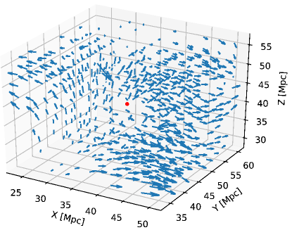
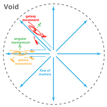
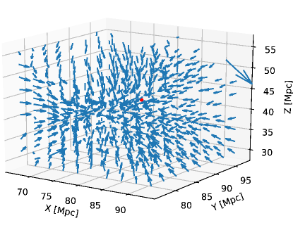
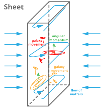
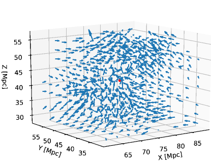
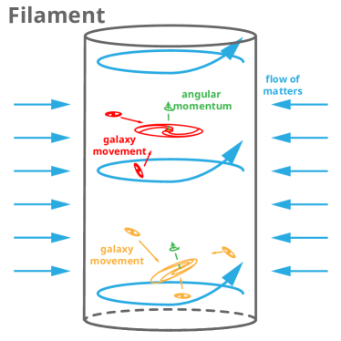
Figure 5: The left column show the velocity field of $10{\rm Mpc}^{3}$ box around center of void, sheet and filament. In the right column, we use cartoons to illustrate the movement of galaxies (red and yellow arrows) and matters in back ground(blue arrows), as well as the possible alignment patterns between central and satellite galaxies. From Top to bottom, each row shows the situation of one environments, i.e., void, sheet and filament. The velocity field of clusters is very messy, thus we don’t show its figures here.

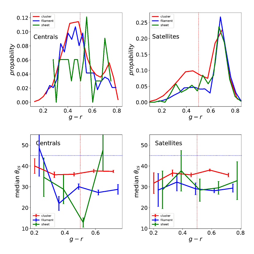
Figure 6: The upper two panels show the distribution of central galaxies’ color (upper left) and satellite galaxies’ color (upper right). Lower panels show the mean alignment angle $\theta_{CS}$ as a function of central galaxies’ color (lower left) and satellite galaxies’ color (lower right). Curves for different sub-samples are distinguished by color as legend shows. Red dotted vertical line shows the division between blue and red galaxies. In lower panels, black dotted horizontal line shows the average alignment angle of random distribution. We don’t show voids galaxies here because there are too less of them. To make the error bars clear, we shift lines a bit horizontally.

To explore the dependence of central-satellite alignment angle on the large-scale environment, we first calculate the median angle in cluster, filament, sheet and void, which is depicted in Figure 4. The exact values of mean angle are given in Table 3.

As shown in Figure 4, the alignment signal are increasing from environments of cluster to filament, sheet, then void. This trend is much more stronger than the results in Wang et al. (2018). Such environmental dependency could be explained by tracing the accretion history in the different large-scale environments (Codis et al. 2012). To illustrate this, we plot Figure 5.

In void, the matters flows radially away from the central region to the surrounding dense region. The velocity field of void in left top subplot of Figure 5 show this trend clearly. During this process, the angular momentum of the gas is thus perpendicular to the radial direction, leading to the axis of the galaxy formed more likely aligning with the same radial direction, as represented by the right top subplot of Figure 5. On the other hand, the galaxies formed in voids always tend to move outward radially, on which the satellite accretions occur. By this way, the alignment of the satellite galaxies is likely to be along the main axis of the central galaxy, producing the stronger alignment signals. Trujillo et al. (2006), Brunino et al. (2007) and Varela et al. (2012) paper found that galaxies at the edge of void have a rotating axis both parallel to the outer boundary of void and perpendicular to the radial direction, which is in agreement with our conclusion.

According to the Zeldovich’s approximation, the gas accretion is always anisotropic and the sheets usually appear firstly during the formation of cosmic web, because there is always one direction along which the matter collapse fastest, corresponding to the maximum eigenvalue of the deformation matrix, so as to form a 2-dimensional pancake firstly, i.e., the sheet structure. While accreted onto sheets from both sides, the gas almost keeps its angular momentum parallel to the plane of sheets. Consequently, the galaxies formed on the sheet are having their angular momentum parallel to the sheet plane, as the middle right subplot of Figure 5 shows. At meanwhile, the major axis could be either perpendicular (red central galaxy middle right subplot of Figure 5) or parallel (orange central galaxy) to the sheet, else lying in an intermediate state between them. However, for the satellite galaxies, the accretion occurs in the sheet plane where the galaxies are assembled. Therefore, the position vectors of the satellite galaxies are possible to be perpendicular to the major axies of the central galaxy, causing the alignment signals to weaken and $\theta_{cs}$ to increase.

Matter in sheets would collapse further and form filaments. Gas swirl around and flow into filaments to form spirals that having angular momentum aligned along the direction of filaments, as bottom subplots of Figure 5 shows. Therefor newly formed galaxies (usually blue disk galaxies) tend to have their major axis perpendicular to filaments (Codis et al. 2015; Welker et al. 2018). Since galaxies form within the cylinder of filament, they gather together via the direction of filament. We check the entering direction of satellites in filaments. In our samples, $60.7\%$ of satellites have their the angles between their position vectors at entering time and the direction of filaments smaller than $60^{\circ}$. Note that $60^{\circ}$ is the mean value of angle separation for satellites with random distribution in 3-D space. Thus satellites enter their host halo in a direction that is perpendicular to the plane of center galaxy. The alignment signal becomes weaker. However, since the shape of center galaxies make change as they also keep accreting gas from filaments, their major axis will be gradually redirected to the direction of filaments. On the other hand, early accreted satellite galaxies will move closer to major axis of center galaxies when they fall closer to them. Because of above two mechanism, old red center galaxies consequently present stronger alignment signal (Yang et al. 2006; Welker et al. 2018).

In clusters, satellites galaxies are more likely come from the conjunct filaments. However, for individual galaxy, surrounding gas is so defused with complex movement that they could be accreted in any direction. Early formed center galaxies may have their satellites and accreted mass via the same direction. Because at early stage of cluster growing, gas may flow in in the same direction as satellites. For those late formed galaxies, position of accreted satellite could be totally irrelevant to incoming gas.

Above descriptions are favored by many works (e.g., Codis et al. 2012, 2015; Welker et al. 2018). They can well explain the influence of large scale structures on galaxies’ central-satellite alignments. However, the alignment signal in simulation is much stronger than that in observations, which indicates that the simulations might have not fully reconstruct the non-linear process and sub-grid physics such as thermal and kinetic feedback.

When we take views from galaxy color, we found that the dependency on large scale environment is not influenced by the color of centrals or satellites. The curves of sub-samples have nearly the same slope as the black curve of the whole sample, while the amplitude shift keeps almost constant in all environment. Only in voids, the $\theta_{CS}$ of blue centrals fall rapidly while that of red centrals become flat. This sudden change may not be reliable, since the number of galaxy pairs in voids is much less then in other environments.

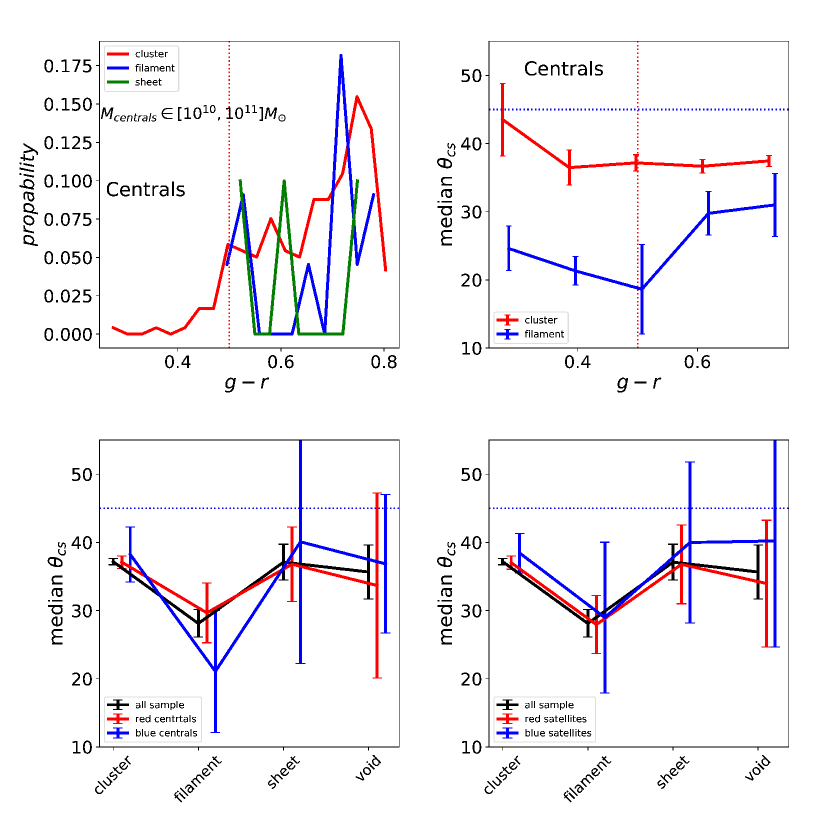
Figure 7: Top left subplot shows the color distribution of central galaxies with mass of $10^{10}\sim 10^{11}{\rm M_{\odot}}$. The pattern is the same as top left subplot of Figure 6. Other subplots show the alignment of galaxy pairs with central galaxies within the same range. Top right subplot show the relation between median alignment angle and color of central galaxies, which is the same as bottom left subplot in Figure 6. The curves for sheet and void galaxies are not shown because the there are few samples. Two bottom subplots shows the alignment-environment relation for galaxies with different colors, which are the same as top rows in Figure 4.

Most parts of these $\theta_{CS}$-environment curves have the same trends as Wang et al. (2018)’s work. In their results, the alignment of blue centrals is strongly dependent on environment, while red centrals does not. For the EAGLE galaxies, blue and red centrals have same $\theta_{CS}$ in clusters, while SDSS DR7 data shows significant discrepancy between red and blue centrals in clusters.

We also investigated the color dependence on the environments. We found a blue biased center galaxy group, as Figure 6 shows. The galaxy color distribution is almost the same in cluster, filament and sheet, except that satellites in clusters have an extra peak in blue region. This distribution is totally different from SDSS data (Wang et al. 2018). In Wang et al. (2018), the probability distribution of central galaxies has its peak at the red part, and the fraction of blue galaxies increases from clusters to sheets. In the lower panels, we found that $\theta_{CS}$ is independent on $g-r$ in clusters. In filaments $\theta_{CS}$ decrease slightly with galaxies’ color. The relation become unstable in sheets due to the limited galaxy number. In Wang & Kang (2018), the alignment-color relation has steady falling trend in all environment, and the slopes are identically the same.

We have found that EAGLE galaxies do not fully recover the color distribution as observations. However we could not say that this is the only reason for the inconsistences of the color dependence of alignment-environment relation between this work and Wang et al. (2018). Guo et al. (2016) claimed that, in EAGLE simulation, the passive fraction of galaxies with mass between $10^{10}$ to $10^{11}{\rm M_{\odot}}$ is quite reasonable compared with observations. Thus we further check the alignment of galaxy pairs with central galaxies within this range. The top left subplot of Figure 7 shows that, for specific central galaxy mass range, the color distribution is much more closer to observations (see Figure 3 in Wang et al. (2018)). But top right subplot tells us the $\theta_{cs}$ - $(g-r)$ relation of this sub-sample is still inconsistent with Wang et al. (2018)’s results. Moreover, the alignment angle is less related with environment for both blue and red galaxies, while in observations blue centrals have stronger alignment signal than reds (Wang et al. 2018). Such differences imply that, even for galaxy catalogue with right color distribution, the alignment - color relation is not well recovered due to some sophisticated sub-grid physics.

3.3 LSE at High Redshift

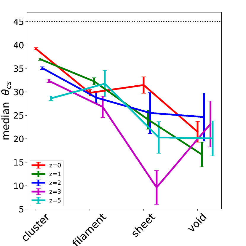
Figure 8: Alignment angle distribution in different environments at different redshifts. Alignment-environment relation curves for different redshifts are distinguished by different color as legend shows. Black dashed line at $\theta_{CS}$ indicates the alignment angle of random distribution. To make the error bars clear, we shift lines a bit horizontally.

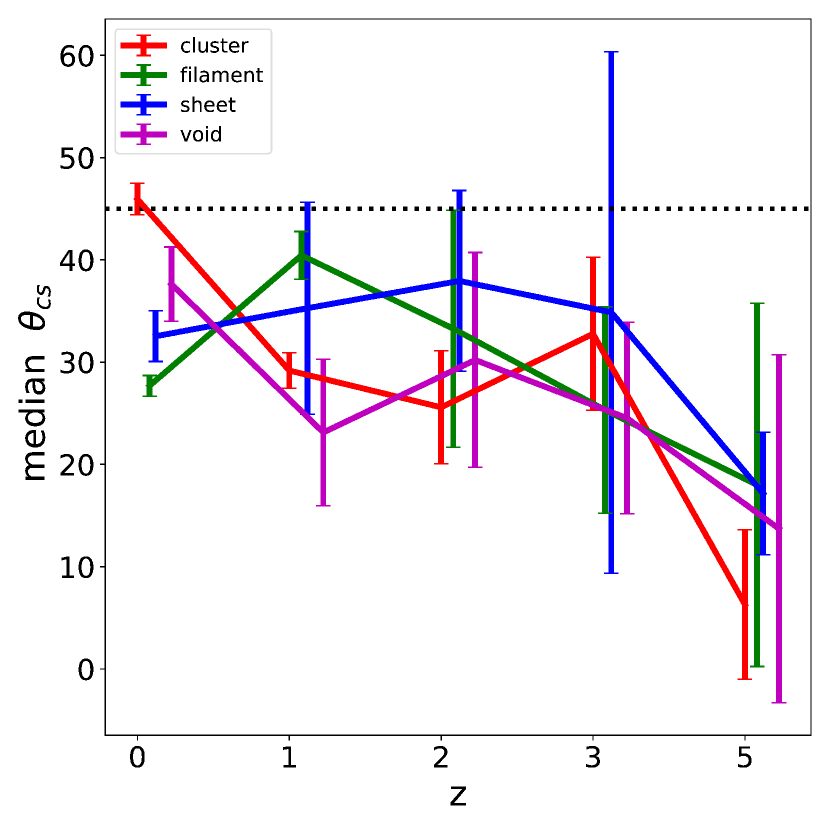
Figure 9: The change of mean alignment angle of galaxies in four dark matter halos. Four halos are selected from different large scale structures, i.e., cluster, filament, sheet and void. Each line shows the statistic of galaxy alignment between one center galaxy and its satellite galaxies. To make the error bars clear, we shift lines a bit horizontally.

In order to investigate the evolution of the alignment angle, we also calculate the alignment angle at higher redshifts, e.g. $z=1,2,3,5$, Figure 8 illustrates the probability distribution of the alignment angle at those redshifts. We found that the alignment-environment correlation exists at all redshifts. The strength of the alignment signal increases from clusters, filaments to sheets then voids. The slopes of those curves at different redshifts are quite close, implying that the difference between structures does not change significantly for a long time. As we have mentioned in section 3.2, the alignment comes from the different mass accretion paths both of central and satellite galaxies. A reasonable scenario is that the mass accretion follows the different paths in the different large scale environments, resulting in the environmental dependency of the alignment. Thus we would expect environmental dependency of alignment at any time that large scale structures exists.

In clusters, central-satellite galaxy pairs show stronger alignment signal at higher redshifts. This evolution trend still exists in filaments, but become merely observed in sheets and voids. It is found that early accreted satellites, in another words, satellites closer to the center galaxies, prefer to align along the galaxies’ major axis (Yang et al. 2006; Faltenbacher et al. 2008; Wang & Kang 2018) . One possible explanation is that the satellites move closer to the major axis after falling into their host halo (Welker et al. 2018) . However our Figure 8 implies another possible routine: early accreted satellites tend to enter their host halos in paths that are closer to the major axis than those entering late. Late accreted satellites dilute alignment signal resulting in increasing average $\theta_{CS}$.

To confirm which process dominates the evolution of central-satellite alignments, we choose 4 central galaxies to trace how the alignment angles of their satellites evolves with redshifts. These four center galaxies are deliberately chosen from the four different structure types. For each central galaxy, we calculate the mean $\theta_{CS}$ of its satellites at each snapshots, then plot $\langle\theta_{CS}\rangle$ versus $z$ in Figure 9. In Figure 9, $\langle\theta_{CS}\rangle$ of cluster galaxies decreases from $z=0$ to $z=5$. It supports our previous assumption that the early accreted satellites was accreted closer to the major axis of central galaxy than the late accreted ones. The filament, sheet and void galaxies do not have monotonic evolution change curves. That is why we did not observe alignment angle weakening with time in other structures except clusters.

4 Conclusion and Discussion

Using data from EAGLE hydrodynamic simulation, we explore the large-scale environment dependence of the alignment angle between central galaxy major axis and satellite galaxy position vector. This is mainly a follow up work of Wang et al. (2018), thus all results are compared with their results based on SDSS observation data. The general conclusions are summarized below:

• In consistent with the results in Wang et al. (2018), the alignment signal between the major axis of central galaxies and the position vector of satellite galaxies in EAGLE simulations exhibits environmental dependence. Average  alignment angle decreases gradually when the environment changes from cluster to filament, sheet and void. However, the amplitude of alignment signal in simulation, as well as the environmental dependency, are much stronger than results extracted from observations. Further improvements on the sub-physics of simulation may overcome this discrepancy. It is also possible that observational contamination dilute the alignment signal.

• We found that EAGLE galaxies don’t recover the dependency of alignment on galaxy color. The fact that EAGLE produces more blue central galaxies than observations takes part of emergence of this bias. However, the trends are not right even for sub-samples with right color distribution. It is possible that the color of both red and blue galaxies is wrongly assigned. To testify it, a through investigation into sub-grid physics is required in future works.

• We found that the influence of large scale structures exists at high redshifts. It demonstrates that the phenomenon of alignments of satellite galaxies is mainly dynamically driven process which is largely determined by the flows of matters.

Comparing with the alignment signal extracted from observations in Wang et al. (2018), there are main two differences in our results: the alignment signal is too strong, and galaxy colors are mis-assigned. However, it is still worthwhile to consider the large scale structure effect on alignment within the scope of simulations. The simulation basically reproduce the trends for overall alignment signal as well as for the dependency on large scale environment. Since the dynamic processes of simulations is promising, we could explore the inner driven for large scale structure dependency. And we confirm that the alignment signal reported in this work and Wang et al. (2018) can be explained by the matter accretion scenario proposed in previous works Codis et al. (2015, 2012); Welker et al. (2018).