FAKIR : An algorithm for revealing the anatomy and pose of statues from raw point sets

Abstract

3D acquisition of archaeological artefacts has become an essential part of cultural heritage research for preservation or restoration purpose. Statues, in particular, have been at the center of many projects. In this paper, we introduce a way to improve the understanding of acquired statues representing real or imaginary creatures by registering a simple and pliable articulated model to the raw point set data. Our approach performs a Forward And bacKward Iterative Registration (FAKIR) which proceeds joint by joint, needing only a few iterations to converge. We are thus able to detect the pose and elementary anatomy of sculptures, with possibly non realistic body proportions. By adapting our simple skeleton, our method can work on animals and imaginary creatures. <ccs2012> <concept> <concept_id>10010147.10010371.10010396</concept_id> <concept_desc>Computing methodologies Shape modeling</concept_desc> <concept_significance>500</concept_significance> </concept> <concept> <concept_id>10010147.10010371.10010396.10010400</concept_id> <concept_desc>Computing methodologies Point-based models</concept_desc> <concept_significance>500</concept_significance> </concept> </ccs2012> [500]Computing methodologies Shape modeling [500]Computing methodologies Point-based models

1 Introduction

With the progress of 3d scanning techniques, it is now common to create digital replicas of artworks, which will remain forever intact, while their real-world counterparts will slowly decay due to time damage or human activity. As part of the automatic processing of scanned statues, it is often necessary to identify the pose and anatomy of the model. Indeed, registering a model to a statue is useful for many applications. For example, one can bring statues to a common pose to better compare their style. It can also serve to combine statue parts to restore broken statue virtually or to animate a statue.

While pose recognition has been efficiently addressed for human models, in particular using Machine Learning algorithms, these methods can only work if the model fits the training dataset of shape models. A challenge of artistic human statues compared to real human scans lies in the difference in aesthetic perception. Indeed many sculptors favored the perceived beauty of their work over the realism of human proportions [Hus55, New34]. As we will see, this has drastic consequences for example-based machine learning algorithms, which fail at adapting to these statues. As for imaginary creatures, no such training database exist. Hence there is a need for simple anatomical models, that can be fitted without requiring an extensive training on various creatures, animals or humans with nonrealistic body proportions.

In this work, we focus on human statues with no or few garments, animals, and imaginary creatures. Furthermore, we consider that the digitized statues are provided as point sets. We propose a method for calibrating and registering a simple articulated model to a point set, which we named Forward And bacKward Iterative Registration (FAKIR). FAKIR works directly on the point cloud, avoiding thus the tedious meshing step. FAKIR iterates between assigning each point to its best corresponding model part and optimizing the anatomical model pose and proportions accordingly, and converges in only a few iterations.

To summarize, our contributions are the following:

• A simple articulated model efficiently representing a statue pose and anatomy.

• An efficient calibration and registration process based on inverse kinematics principles.

2 Related work

Anatomical Model.

Designing anatomical models for human shapes has raised a lot of interest in Computer Graphics. The most common representation consists in a more or less detailed graph of bones such as the ones used in the MakeHuman framework [Bas00], while some methods go beyond this kind of elementary skeleton representation and model every single muscle to increase realism [LGK^∗12]. Due to our nonrealistic context, we will focus here on basic skeletons, which are pliable and efficient enough for our purpose. A skeleton-based model consists of two components: a skeletal structure [BK00] and a representation for the volume surrounding it. This representation can be either mesh surfaces or volumetric primitives. Recent surface-based models [ASK^∗05, PMRMB15, LMR^∗15, HSS^∗09, ZB15] are learned from numerous scans of real people. Among those, SMPL  [LMR^∗15] is a human anatomical mesh model in which a set of parameters control non-rigid deformations resulting from a statistical study on a large number of humans and positions. However, to our knowledge, there is no approach that allows us to position this model from a static point cloud without positioning the model close to the data or without using 2D views and deep learning. It works well for the capture of human motion and shape in a video [ZPBPM17] or images [BKL^∗16, HBL^∗17]. But this model has a poor performance when the data is unrealistic which is common for archaeological statues. Another possible shape representation is based on volumetric primitives, e.g. using medial axis transform (MAT) [Blu67, SCYW16], metaballs [PF01], B-meshes[JLW10] or other primitives [GD96, SBR^∗04, ARM^∗19]. Among these models, the sphere-mesh model [TGB13], a variant of convolution surfaces [BS91], has been introduced for representing mesh models by packing spheres into it and encoding their structure. Conceptually, the sphere-mesh model can be seen as a piecewise linear simplification of the computational geometry skeleton [TDS^∗16]. Although sphere-meshes were developed to extract the shape structure from an input mesh, they can be used to represent an anatomical model by imposing constraints on them. As such, it has been used successfully for representing hand skeletons [TPT16, RTTP17]. This model is light and pliable and we will also rely on it.

Skeleton registration

Registering a model to a shape is an important task which has received much research interest. The goal can be to animate a shape by skeleton rigging and skinning, or to detect human poses. Skeleton rigging can be performed manually [BK00, JLW10], but a few methods have investigated automatic processes. In particular, the Pinocchio algorithm [BP07] adapts a skeleton to a static mesh by defining an objective function and maximizing it. It works by packing spheres into the mesh and by considering their centers, gathered in a graph, as the admissible joint positions. This pre-computation makes the skeleton pose estimation tractable. On points sets, a $\ell^{1}$-medial skeleton could be used [HWCO^∗13] alternatively to sphere-packing, but it is not suitable for noisy or incomplete data, as shown by our experiments. If the input data is dynamic, it is possible to infer, or track, a skeleton from it. Most tracking approaches [SBB10, GSA^∗09, TZMS04] focus on the capture of the positions of the joints, and deduce pose parameters (angles) and intrinsic parameters (e.g. bone lengths) from it. Many of such tracking methods [SHG^∗11, WZC12] start with a calibrated skeleton but the calibration itself can be performed from a depth video and a set of known admissible poses [TPT16, RTTP17, TTR^∗17]. Such methods require a dynamic scene and cannot apply to the static shape rigging problem. It is also possible to rely on a database of people scans to learn the pose and deformation of human bodies using the SMPL model [HLRB12, WHB11, AMX^∗18]. Recently, CNN-based detectors, such as DeepCut[PIT^∗16] and OpenPose[CHS^∗18] were used for 2D joints detection in images or videos. Bogo et al. [BKL^∗16] estimate the 3d human pose and proportions from a single image by fitting a SMPL model to DeepCut estimated joint positions. Using multi-view images over time [HBL^∗17] improves the pose accuracy, however the human proportions remain approximate. Human tracking can also be done without needing a model [BBLR15]. Similarly it is possible to register two models using manifold-harmonics based non rigid registration [LRB^∗16], but this would not help for skeleton-based registration. Learning approaches can also work from a single image [LIPM19, AMB^∗19].

Registering an SMPL skeleton directly to a point cloud has been addressed using deep learning directly on point sets augmented with feature detection [JCZ19], but this method only targets human shapes, which it learns from a database, while our method can work on nonrealistic anatomies and on various animals, as will be demonstrated in our experiments. Deforming a point cloud to match a template mesh has also been tackled using auto-encoders [LSS^∗19], but this requires a full template mesh for each model. Our required skeleton model is much lighter. Finally, recently, the FARM[MMRC20] method builds on the functional map framework to register a parametric model (such as the SMPL one) to a mesh or a point set in a fully automatic way. This approach reaches state of the art results while being the closest in goal to ours, and we will compare to it.

Finally, some methods [HSR^∗09, ZPBPM17, PMPHB17, YZZ^∗19] aim at finding a person’s pose despite its sometimes loose clothing, but this is outside the scope of our paper.

Our registration algorithm makes extensive use of kinematic chains, processing them alternatively forward and backwards. In spirit, this is related to inverse kinematics, and in particular the Fabrik [AL11] and CCD [WC91] algorithms. Indeed, both methods define kinematic chains and compute their transformation from an input pose to a target pose by updating pose parameters one after the other alternatively forward and backward along each chain. However the similarity ends here, since our goal is to estimate not only the pose but also the proportions of the model limbs using data-attachment constraints in a static framework.

3 Anatomy and Pose estimation

3.1 Human model

In our context of artistic statues, it is necessary to devise a human model with few constraints, allowing to fit a sculpture which does not follow the human proportion beauty canons. The existing fully detailed human templates modeling every single limb and muscle in a very realistic way are too constrained for our purpose.

We introduce an anatomical model inspired by the sphere-mesh model [TGB13], already successfully used for hand tracking [TPT16, RTTP17], using only one-dimensional elements. In this model, each bone is represented by a sphere-mesh $B$ corresponding to the envelope of the union of a set of spheres centered on a segment and with a linearly varying radius (Figure 1(b)). Each bone is defined by two end sphere centers $c_{1}$ and $c_{2}$ with associated radii $r_{1}$ and $r_{2}$ respectively. The segment $[c_{1}c_{2}]$ is the medial axis of the bone. For each point $c\in[c_{1}c_{2}]$, the radius of the sphere centered at $c$ is $r(c)=(1-\tau)r_{1}+\tau r_{2}$, with $\tau=\frac{\|c_{1}c\|}{\|c_{1}c_{2}\|}$.

The sphere-mesh model is controlled by the length $l=\|c_{1}c_{2}\|$ and the pair of sphere radii $\mathbf{r}=\{r_{1},r_{2}\}$. Consequently, we denote the sphere-mesh model for one bone as $B(l,\mathbf{r})$. We also denote by $\alpha$ the angle of the conic part of the bone, as illustrated on Figure 1(a). Importantly enough, the bones we are defining do not correspond to anatomical bones, but more to limbs (i.e. it includes a coarse description of the flesh volume around the anatomical bone). By analogy to inverse kinematics, we keep the word bone instead of limb.

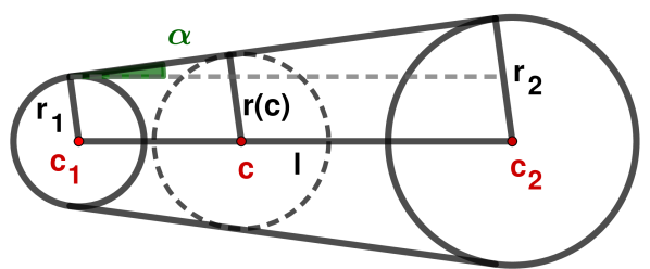
(a) Cross-section of a bone

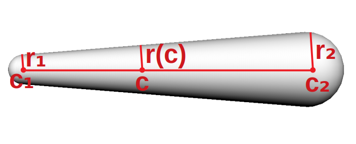
(b) Sphere-mesh of a 3D bone.

Figure 1: The sphere-mesh of a bone is the union of the spheres centered on segment $[c_{1}c_{2}]$, with radius varying linearly between the two extremities of the segment.

With this type of bone element, we construct a simple human body template with a very coarse respect of human proportions as an initial body shape (Figure 2(a)) but we can construct a template for any other animal or imaginary creature (Figure 2(b)) as well. Our human body template contains 22 bones $\{B_{k}\}_{k=1..22}$. Three of those correspond to the pelvis and have no relative motion: their length is fixed up to a common scale parameter that will be determined during the registration, along with the orientation of the triplet. Additionally, a special bone is used to connect the spine bone to the neck, and its length and orientation directly depend on the adjacent spine bone. The other bones have no constraint on their relative proportions. The bones are organized into 5 chains, depicted in different colors in Figure 2. These chains are independent with the only constraint that some extremities must remain anchored to the spine. The orientation of the chains is used to define the predecessor and successor of each bone. The ordering will be reversed to process the chain forward and backward several times during the registration process. Each bone is thus fully defined by its intrinsic parameters (length and two radii) and by its extrinsic parameter (rotation with respect to its predecessor). Because of the simplicity of the sphere-mesh bone model, the distance from a point to the model can be easily computed. In contrast, using a mesh model would make these computations much more demanding.

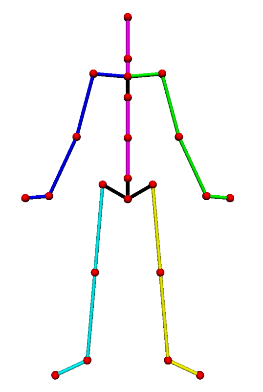
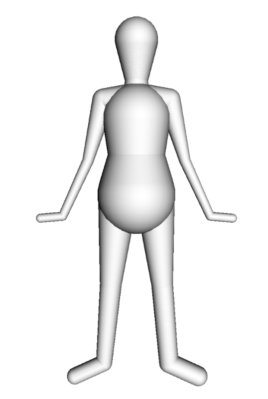
(a) Human model

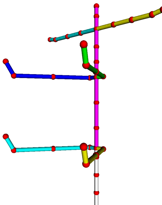
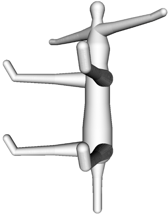
(b) Centaur model

Figure 2: Skeleton and sphere-mesh models for humans and centaurs. For the human model: the bones are organized into 5 chains shown in different colors. $4$ additional bones are drawn in black: the pelvis which is a constrained triplet of bones, and the connection bone between the spine and the neck. Our model can also be adapted to various creatures, even imaginary ones such as a centaur.

3.2 Distance between the model and a point set

To capture the anatomy and the pose of a statue, we need a distance function to measure how the sphere-mesh model fits a point set $P$, even if the points are far from the bones they should be attached to. The sphere-mesh model calibration and registration strives to reduce the distance between the sampled points and their corresponding bones on the sphere-mesh. The problem is that the bone to which a point should be assigned is unknown, especially if the model has not been calibrated beforehand and if it is far from the data. Therefore, the target bone is usually replaced by the closest bone. We assume that the coordinates of the points are provided with a coarse approximation of the oriented normal. This speeds up the registration when the model is not close to the data, but it remains possible to implement our registration algorithm with a simple Euclidean distance from the points to the model.

Distance from a point to one bone.

We start by defining the normal-constrained projection of a sampled point $p$ on a single bone $B$ by using the oriented normal vector $\mathbf{n}_{p}$ to disambiguate the choice between several orthogonal projection possibilities. Given a point $p$ in the ambient space with oriented normal $\mathbf{n}_{p}$, we consider the lines passing through $p$ and orthogonally intersecting the sphere-mesh surface (possibly crossing its interior) at some points.

Whenever it is possible, we select the projection $\tilde{p}$ whose normal $\mathbf{n}_{\tilde{p}}$ has positive scalar product with $\mathbf{n}_{p}$. Considering this normal-constrained orthogonal projection allows for a faster convergence and better results (see the supplementary material for more details). Since each point $p$ has a normal-constrained projection on all the bones, we refer to its normal-constrained projection on bone $B_{k}$ as $\tilde{p}_{k}$. If no subscript is provided, $\tilde{p}$ refers to the normal-constrained projection of $p$ on the closest bone.

Distance from a point set to a sphere-mesh chain.

Given a point set $P$ and a sphere-mesh chain of $K$ bones, we first need to approximate the subset of current points that project on each bone. In the following, we define the point set $P_{k}$ as the subset of points $p\in P$ which are closest to bone $B_{k}$ using the distance $d_{k}=\|p-\tilde{p}_{k}\|,k=1\cdots K$. Once the assignment is computed, the one-bone distance function $E_{k}$ is defined as the sum of squared distances from points of $P_{k}$ to bone $B_{k}$:

$$E_{k}(P_{k},B_{k}(l_{k},\bm{r}_{k}),\bm{\theta}_{k})=\underset{p\in P_{k}}{\sum}\|p-\tilde{p}_{k}\|^{2}$$ (1)

Importantly enough, the subset $P_{k}$ and the one-bone energy $E_{k}$ depend on the position of the initial extremity of the chain of bones involving $B_{k}$, as well as the parameters of the other bones in the chain.

The sum of one-bone distance functions measures the fitness of the model and serves as an objective function that we aim to minimize in order to capture the anatomy and pose of the sphere-mesh that best corresponds to our point set.

$$E=\sum_{k=1}^{K}\sum_{p\in P_{k}}\|p-\tilde{p}_{k}\|^{2}.$$ (2)

In the next sections, we will also be interested in the distance restricted to two adjacent bones $B_{k}$ and $B_{k+1}$, which we call two-bones energy:

$$E_{k,k+1}=\sum_{p\in P_{k}}\|p-\tilde{p}_{k}\|^{2}+\sum_{p\in P_{k+1}}\|p-\tilde{p}_{k+1}\|^{2}.$$ (3)

3.3 FAKIR : Forward And bacKward Iterative Registration

To register our anatomical model, we propose a kinematic approach taking into account the way the model is articulated. Contrarily to many methods that work from videos or multiple views [TPT16, RTTP17], our method requires only one joint center to be close to its optimal position, the rest of the skeleton pose being arbitrary. Inspired by the FABRIK [AL11] and CCD [WC91] algorithms, our registration algorithm successively loops forward and backward through the chains of bones so as to rotate and scale them to match the data, refining the parameters while temporarily fixing the extremities of some bones. Hence our algorithm is named Forward And bacKward Iterative Registration (FAKIR). An originality of our method is that bones are mainly considered by consecutive pairs, which allows for a more robust estimation of the pose and skeleton parameters along a chain. The optimization of the parameters related to bone $B_{k}$ requires that there are relevant points attracting that bone into the data attachment term, which justifies a special order for the optimizations (see the supplementary for details).

Registration process for a chain of bones.

If the parameters of bone $B_{k}$ have not yet been initialized, and that it is close to a subset of points to which it should ideally be associated, the estimation of the one-bone energy is meaningful and the minimization of this energy can be used to initialize the position and radii of that bone with respect to the data. Our algorithm gradually rotates and scales the current bone $B_{k}$ with respect to its predecessor, updating $P_{k}$ after each step, so that $P_{k}$ gradually contains more relevant points. However, if $P_{k}$ is empty, the bone is first rotated around the three axis until some input points are projected onto it to bootstrap the optimization. Once the position of $B_{k}$ has been approximately found, the algorithm turns to the coarse estimation of the position of $B_{k+1}$. All these computations are driven by the minimization of the one-bone energy. However, the one-bone energy alone might be inefficient to approximate the full length of a bone accurately. To alleviate that, in an intertwined manner, a finer local registration is performed each time two consecutive bones $B_{k}$ and $B_{k+1}$ have been processed, by minimizing the two-bone energy. This process optimizes the common joint position and radius while keeping the two other joints fixed. It is the most important component in our algorithm. Once a chain of $K$ bones has been positioned and scaled over its entire length, we repeat the process forward and backward in the chain in order to further refine the joints positions and radii between pairs of consecutive bones, using only two-bone energies optimizations. Extremity bones are optimized based on the one-bone energy after each forward or backward pass. The full process is summarized in Algorithm 1 and illustrated with a chain of three bones in Figure 3.

Notice that if two limbs are aligned, the joint position can not be guessed from the data and it may cause several limbs to be included in a single primitive of our sphere-mesh. To avoid this, very loose constraints on the differences in proportions between consecutive bones can be set.

Algorithm 1 Forward and backward iterative registration

0:  A point set $P$ and a sphere-mesh chain of $K$ bones with one chain extremity close to its optimal position

0:  The registered sphere-mesh chain.

1:  Initialization:

2:  Fix the center of the first extremity of the chain. Rotate the first bone and adjust its radii and length by minimizing the one-bone energy;

3:  for $k:=1$ to $K-1$ do

4:     Consider the pair of bones $B_{k},B_{k+1}$ :

5:     Fix the position of the joint common to $B_{k}$ and $B_{k+1}$;

6:     Alternate between the optimization of $B_{k+1}$’s rotation w.r.t $B_{k}$, optimization of $B_{k+1}$’s intrinsic parameters and update of $P_{k+1}$;

7:     Fix the positions of the 2 joints that $B_{k}$ and $B_{k+1}$ do not share, and free their common joint;

8:     Compute the position and the radius of the common joint by using the two-bones energy.

9:  end for

10:  Compute the length of the last bone and the radius of the last sphere.

11:  Forward and Backward registration loop:

12:  repeat

13:     Reverse the order of the bones in the chain;

14:     for $k:=1$ to $K-1$ do

15:        Consider the pair of bones $B_{k},B_{k+1}$ :

16:        Fix the positions of the 2 joints that $B_{k}$ and $B_{k+1}$ do not share;

17:        Compute the position and the radius of the common joint by using the two-bones energy.

18:     end for

19:     Compute the length of the last bone and the radius of the last sphere with the one-bone energy.

20:  until convergence

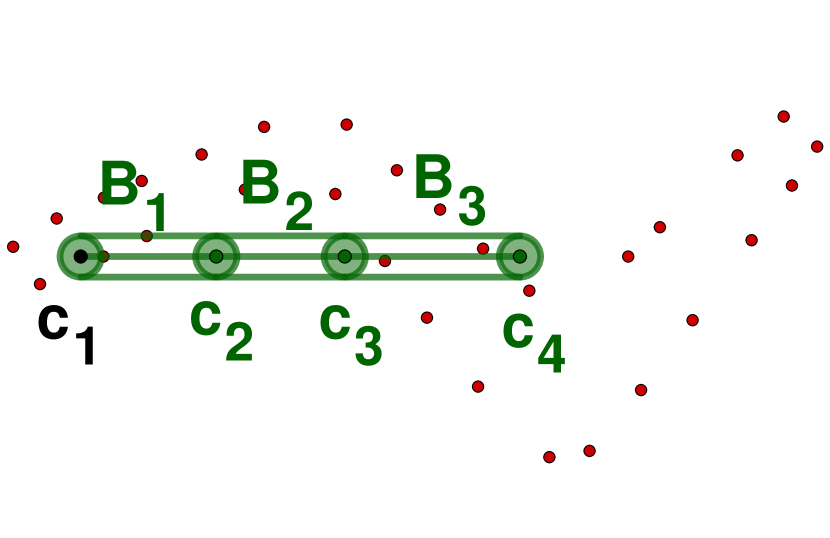
(a)

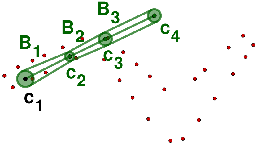
(b)

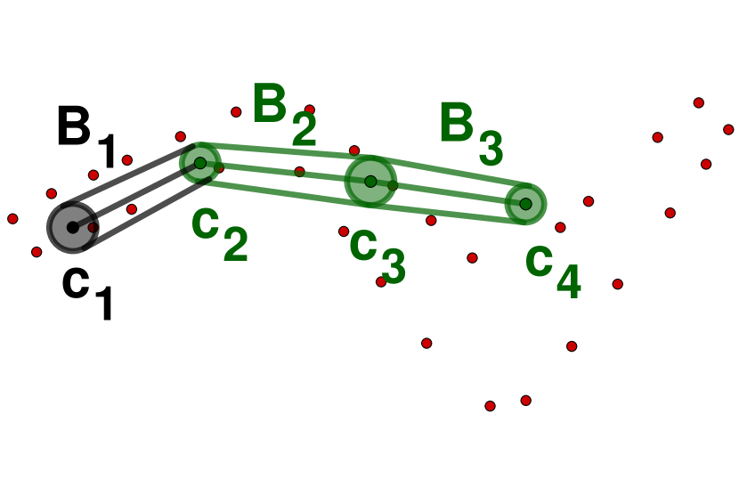
(c)

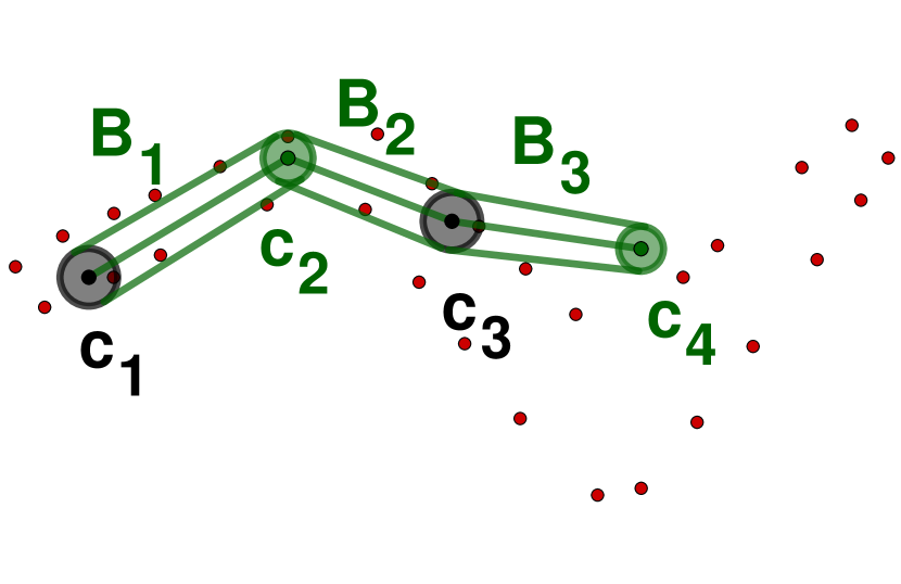
(d)

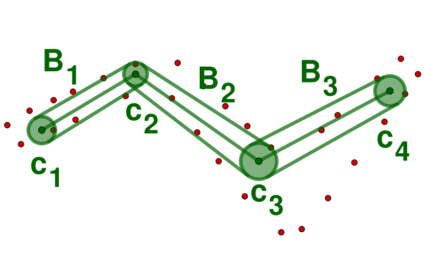
(e)

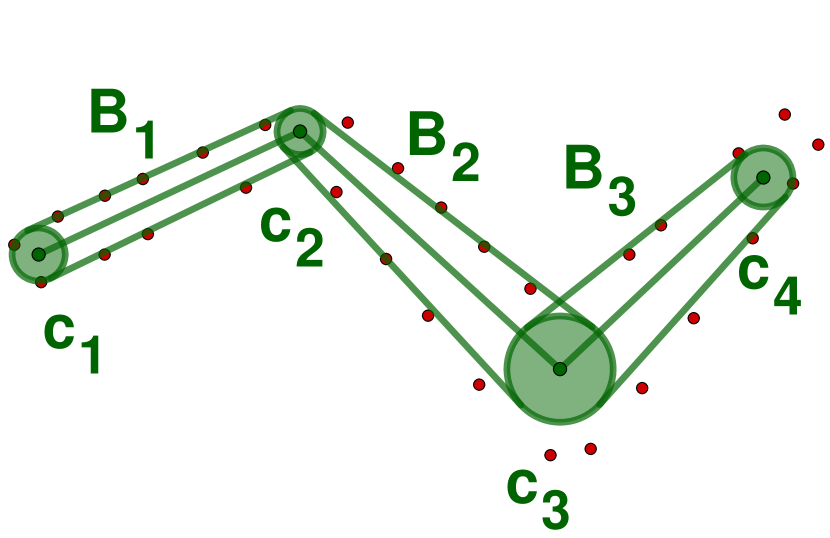
(f)

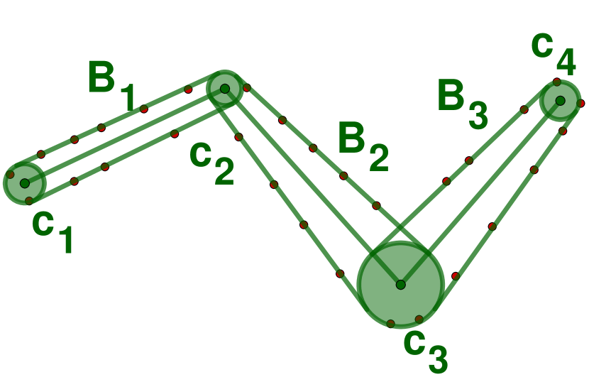
(g)

Figure 3: Overview of the forward and backward iterative registration for a 3-bone chain. From an initial position (a), the chain extremity $c_{1}$ is fixed and the first bone $B_{1}$ is rotated and scaled to roughly calibrate its dimensions and pose through the optimization of the one-bone energy (b); the bone $B_{1}$ is fixed and the parameters of the second bone $B_{2}$ are roughly calibrated in turn (c); joint $c_{2}$ which is common to the first two bones is scaled and its position is optimized, by using the two-bones energy, the other joints being fixed (d); The position and length of the third bone $B_{3}$ are then coarsely calibrated through one-bone optimization and the process continues by alternating single bone optimization and two-bones optimization, until the last bone of the chain (e). After this first coarse calibration forward pass finishes, a backward pass using only two-bone optimizations is performed (f) permitting to refine the pose and skeleton parameters and solve for the chain extremity position. With few forward and backward pass involving two-bone optimization only, the model is registered (g).

Optimization of a single bone

As stated above, the optimization of the one-bone energy is only used for estimating the parameters of the extremities of a chain, or for the very first forward pass in Algorithm 1.

In the single-bone case, the aim is to estimate the 3D rotation of the bone, its length and the radius of its free extremity by minimizing the one-bone energy $E_{k}(P_{k},B_{k}(l_{k},\bf{r}_{k}),\bm{\theta}_{k})$, where $\bm{\theta}_{k}$ are the angles of rotation with respect to the predecessor bone. This optimization is performed using the Levenberg-Marquardt algorithm for each parameter. In particular, the rotation can be decomposed into two rotations around two axes that are orthogonal to $c_{k}c_{k+1}$, indeed the rotation around $c_{k}c_{k+1}$ is not considered since it leaves the bone unchanged. To optimize $\bm{\theta}_{k}$, we iteratively look for the best angle $\bm{\theta}_{k}+\delta\bm{\theta}_{k}$. At a minimum, $\nabla_{\delta\bm{\theta}_{k}}E_{k}(P_{k},B_{k}(l_{r},\bm{r}_{k}),\bm{\theta}_{k}+\delta\bm{\theta}_{k})=\bm{0}$, and the value for $\delta\bm{\theta}_{k}$ follows. The details for the damped least-squares estimation are provided in the supplementary material for all parameters.

Optimization for the joint between two consecutive bones.

The optimization of the position and radius of the joint between two consecutive bones $(B_{k},B_{k+1})$ is performed by optimizing a set of four parameters in a loop (an angle, two lengths and a radius) minimizing the two-bones energy. The two end-sphere centers being fixed ($c_{k}$ and $c_{k+2}$ in Figure 4), we first compute the optimal rotation of the two bones around axis $c_{k}c_{k+2}$. We then optimize the bone lengths $\hat{l}_{k}=l_{k}+\delta l_{k}$ and $\hat{l}_{k+1}=l_{k+1}+\delta l_{k+1}$ and, finally, the radius of the common joint is computed as $\hat{r}_{k+1}=r_{k+1}+\delta r$. The parameters optimization alternates with a recomputation of point sets $P_{k}$ and $P_{k+1}$, which refines the point-to-bone assignment. The optimization is also performed using the Levenberg-Marquardt algorithm (see the supplementary material for details).

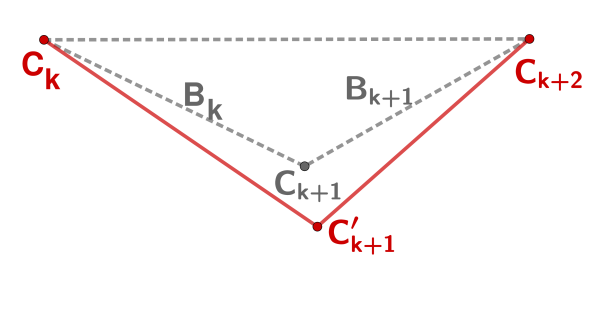
(a) Rotate $B_{k}$ $\cup$ $B_{k+1}$

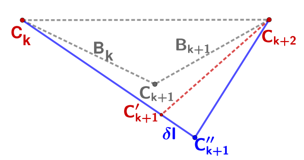
(b) Refine length $l_{k}$ of $B_{k}$

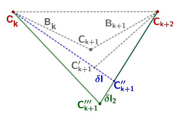
(c) Refine length $l_{k+1}$ of $B_{k+1}$

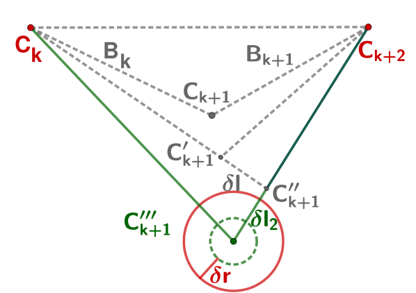
(d) Refine radius $r_{k+1}$

Figure 4: Pairwise Optimization. With fixed extremities $c_{k}$ and $c_{k+2}$, the pair of bones $B_{k}$ and $B_{k+1}$ is first rotated around axis $c_{k}c_{k+2}$. Then the lengths of the bones $B_{k}$ and $B_{k+1}$ and their common radius $r_{k+1}$ are optimized successively. After these updates, the point-to-bone assignment is recomputed. As the process is repeated the distances are more accurate since the point-to-bone assignment becomes more meaningful.

Full Skeleton Registration

The full model corresponds to a tree whose branches are composed of chains. The process of registering each of the chains must be done in such an order that it gradually ensures the relevance of the data attached to each chain. Thus, previously registered chains can be questioned again if their attached points are reassigned to other chains or if they catch new points during the process (see Figure 5).

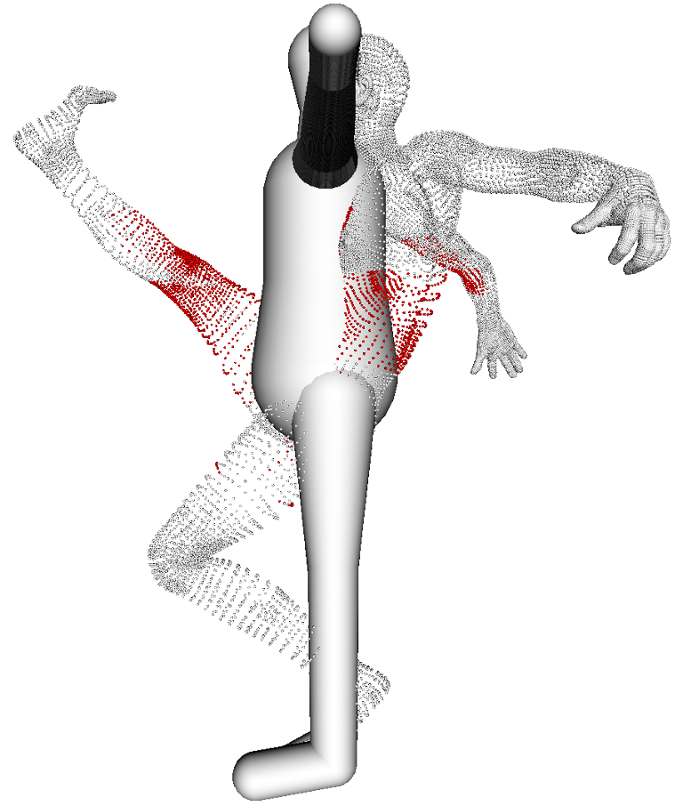
(a) Initialization

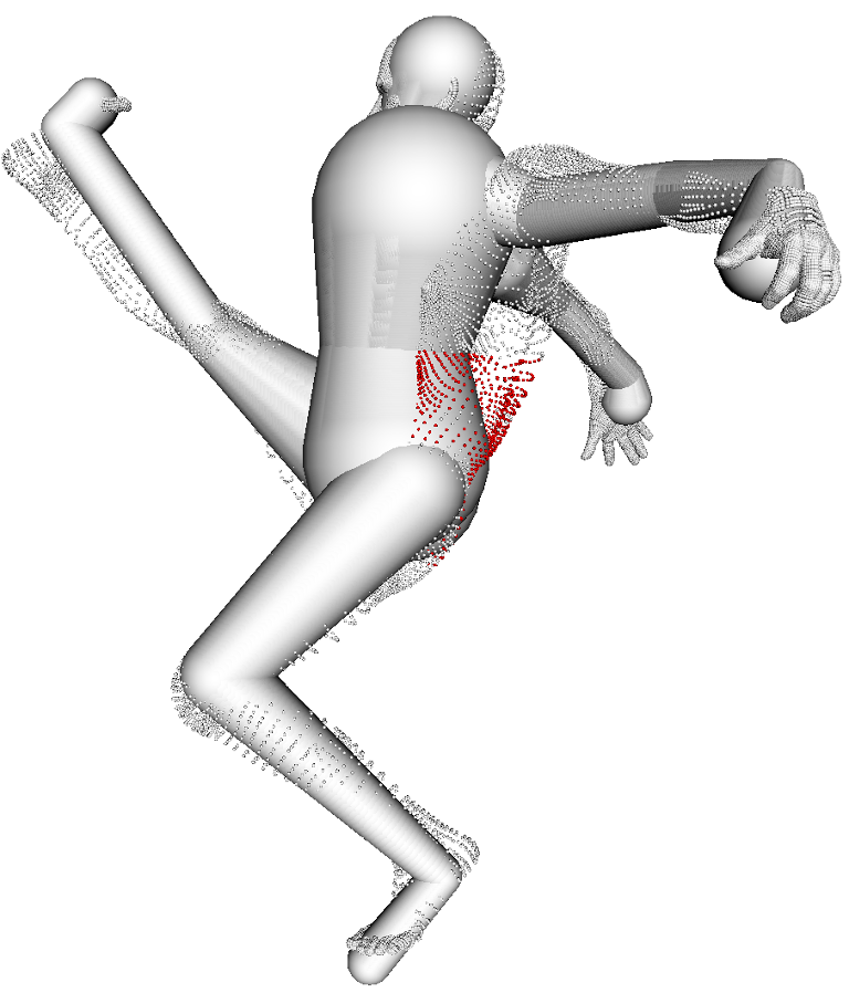
(b) First forward passage

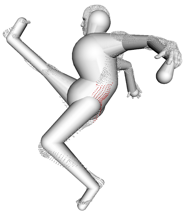
(c) First backward passage

Figure 5: The assigned points for the first spine is showed in red. The spine is first registered with points that are not yet assigned to the legs, which distorts its position. Once the legs are registered, the registration backtracks to the spine and its position can be corrected. The final result is shown on Figure 14.

Our system depends on the initial position of a joint chosen as the root of the skeleton. For example, for human or quadrupeds models, we assume that the pelvis part of our model is initialized near the corresponding part of the point set, which is done manually through a single point and click. Each chain is then registered in turn using FAKIR yielding a registered skeleton both in terms of intrinsic parameters and pose in only a couple of iterations.

For human models, the registration order is the following: first the spine chain is registered, refining the pelvis position and scale during the process, followed by each of the two leg chains and each of the two arm chains. When registering the arms and legs chains, the position for the joint attached to the spine or the pelvis remains fixed. However, after one arm is registered, changing the spine-arm joint position, the spine chain is updated accordingly (and similarly for legs and head), thus the forward and backward chain registration extends to the whole model. This leads to a calibrated and accurately positioned articulated model.

4 Results

In this section, we show the performance of FAKIR both on synthetic data and on point sets resulting from statue digitization. We developed our algorithm in C++, using OpenMP for computing point to bone distances in parallel. All experiments are run on an Intel Core i7-4790K CPU @ 4.00GHz. Normals were computed by using the state of the art approach of Hoppe et al [HDD^∗92].

4.1 Experiments on synthetic data

We first tested our algorithm on synthetic data to provide a quantitative evaluation of the FAKIR performances. We considered a point set of $5k$ points sampled on a sphere-mesh of a 4-bone chain in a specific pose and registered a generic 4-bone chain to it. Although the point set and the initial chain are quite distant from each other, providing an approximate initial position of a single anchor point (one of the extremity) is enough to register accurately the chain. The accuracy of the registration is evaluated as the average distance between the point set and the model.

In the noiseless case, our algorithm takes $7$ iterations to converge to a $0$ distance in $2.37s$, including $0.62s$ for the first forward pass. The distance of the point set to the model with respect to the iterations for larger point sets and increasing noise is shown on Figure 6: the number of points has only a moderate impact on the number of iterations needed to converge (around $7$). When there is noise in the data, the distance also converges in a few iterations independently of the noise, however the distance at convergence is directly correlated to the variance of the noise. As shown by our experiments, FAKIR is rather resilient to even relatively high levels of noise (Gaussian noise in Figure 7 and Poisson noise in Figure 8). Figure 9 shows how FAKIR handles an initial position of the anchor point that is not in the vicinity of its optimal position in the point set. FAKIR can handle initial positions that are moderately far from the true position, but in some cases (last column), the backward optimization of the one-bone energy alone fails to reduce the length of the first bone and the radius of its free extremity degenerates to $0$ instead. This is due to the fact that no point is projected on the spherical free extremity of that bone. This problem could be avoided by adding a bone occupancy term to the one-bone energy. A preferential alternative would be to modify the one-bone energy of the first and last bones by adding a term corresponding to the distance of the free caps to the data points. However, if the initial point is reasonably close to its true position, this problem does not occur. FAKIR is also rather robust to missing data thanks to the iterated forward and backward passes (Figure 10). Naturally when the missing parts are on the first or last bone or when a full bone is missing, the algorithm cannot predict the right length or angle.

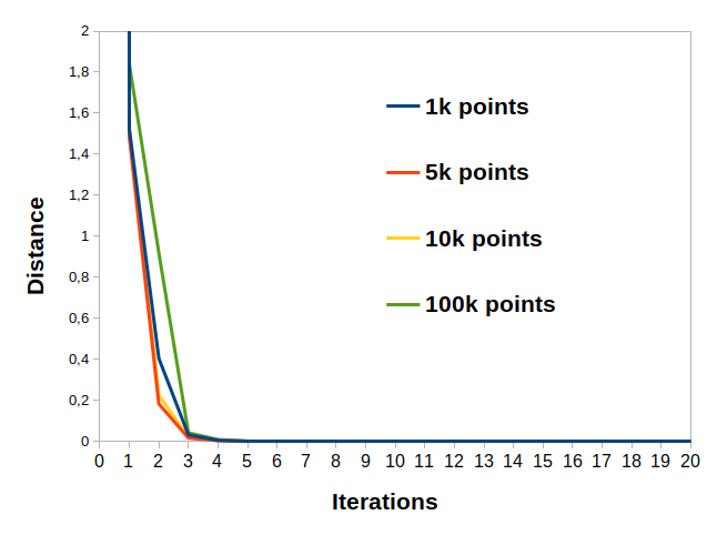
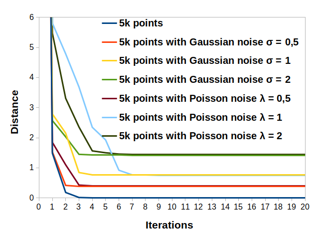
Figure 6: Evolution of the registration distance with the iterations for different number of points in the point set (left image), different levels of Gaussian noise and Poisson noise (right image).

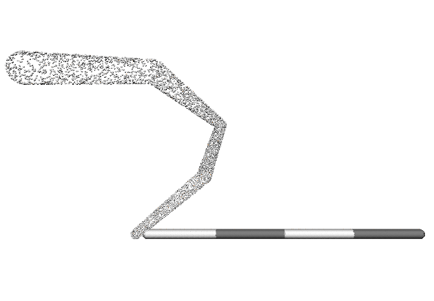
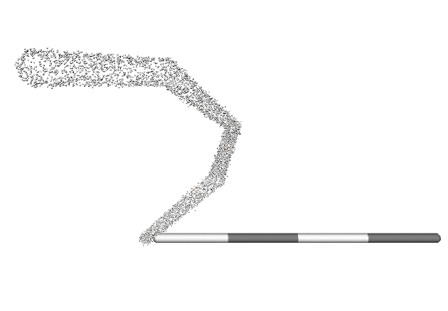
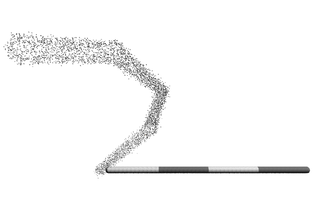
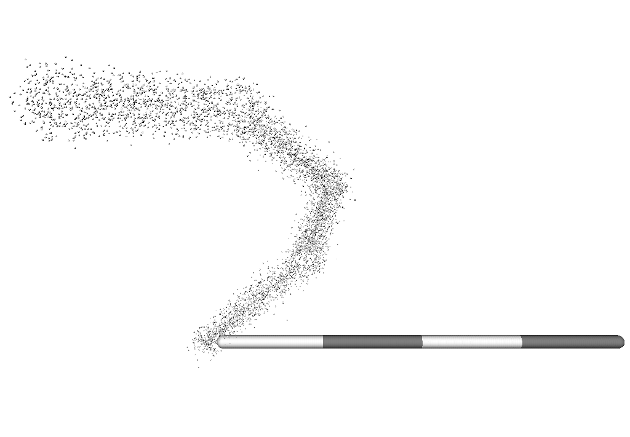
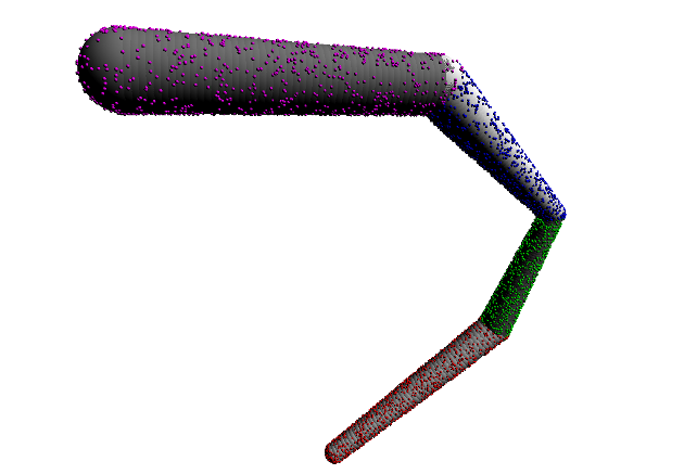
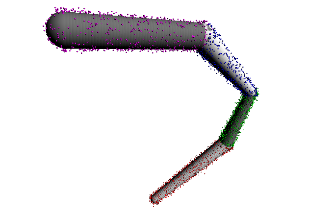
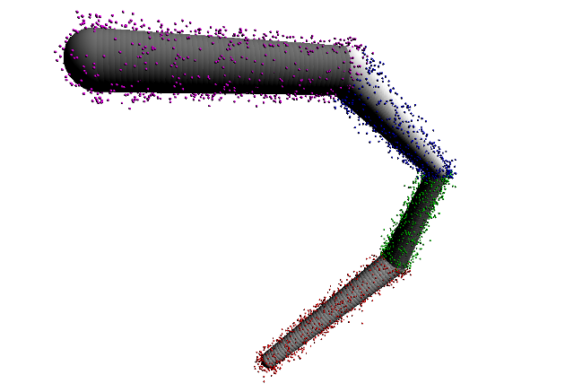
Figure 7: Evaluation of FAKIR with respect to increasing Gaussian noise after $20$ iterations. The first row shows the initial point set and the bottom row shows the registered bone chain. From left to right: without noise, $\sigma=0.5$, $\sigma=1$, and $\sigma=2$. The total groundtruth model length is 140 (All values are given in length units).

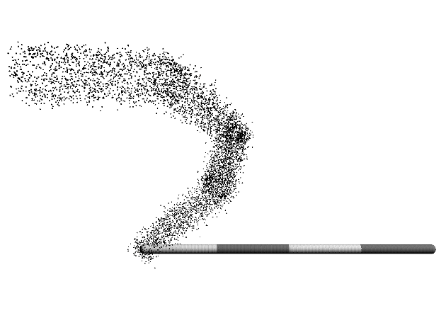
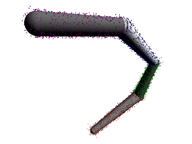
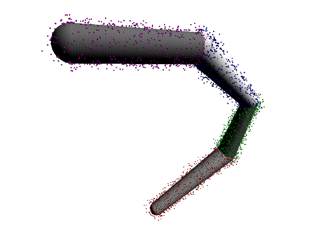
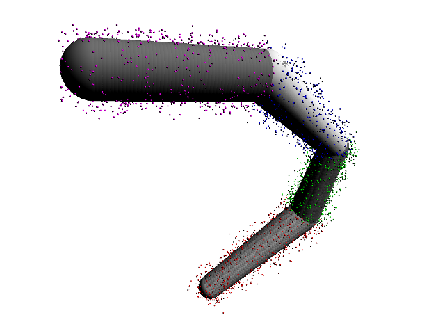
Figure 8: Evaluation of FAKIR with respect to increasing Poisson noise after $20$ iterations. The first row shows the initial point set and the bottom row shows the registered bone chain. From left to right: without noise, $\lambda=0.5$, $\lambda=1$, and $\lambda=2$. The total groundtruth model length is 140 (All values are given in length units).

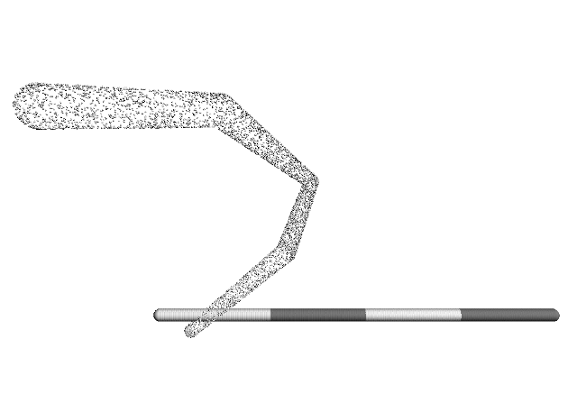
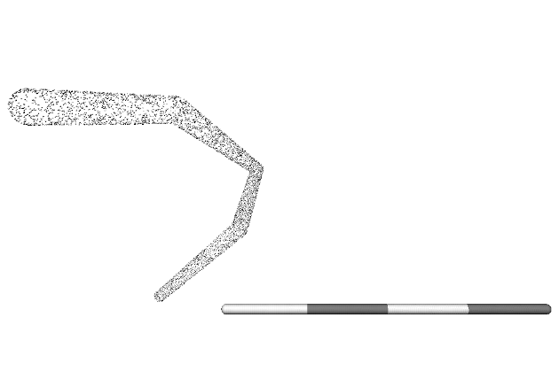
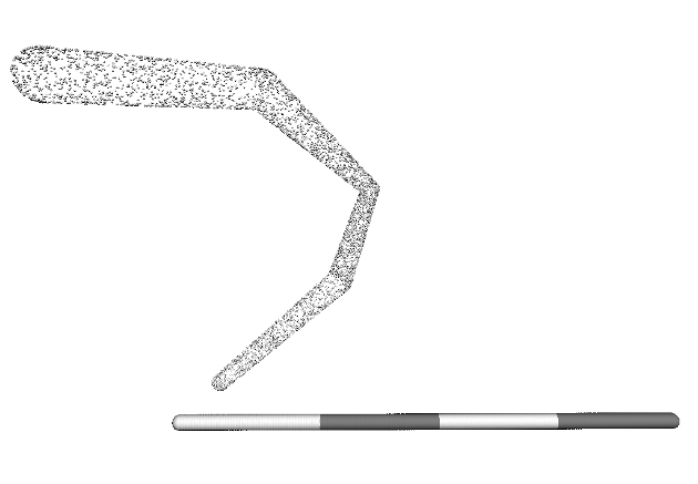
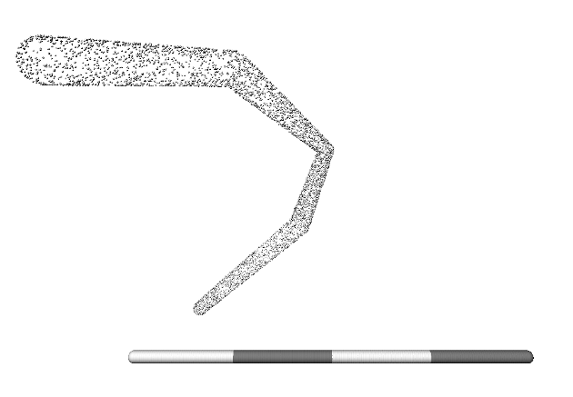
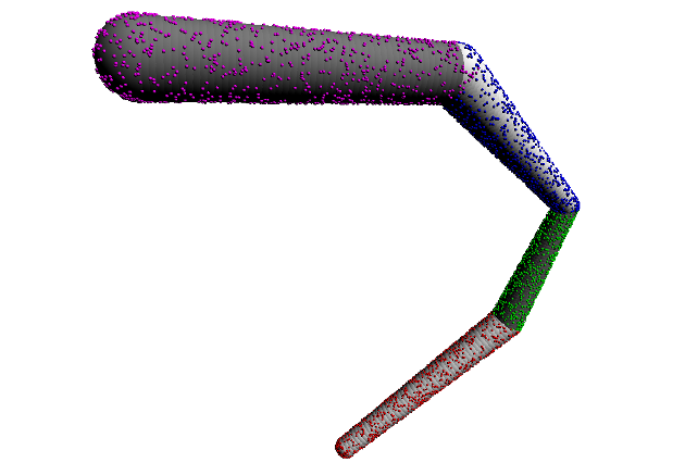
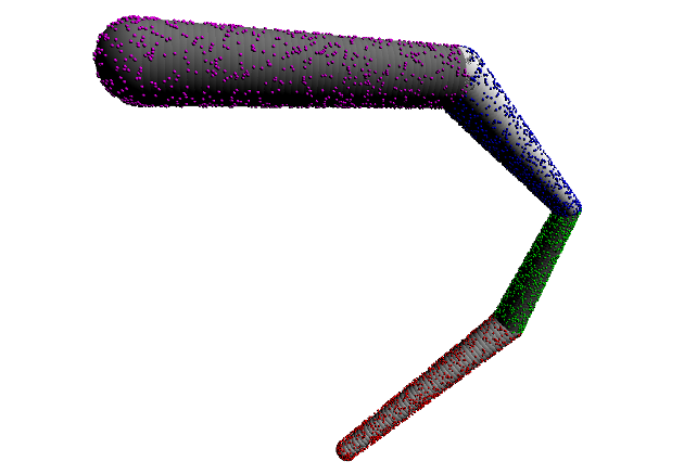
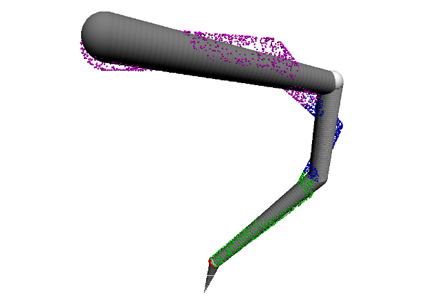
Figure 9: Evaluation of FAKIR with respect to a bad initial anchor point position after $20$ iterations. The first row shows the initial point set and the bottom row shows the registered bone chain. The last column shows that due to a bad initialization, the points (plotted in red) that are affected to the first bone do not bring enough information for the one-bone energy to move the chain extremity. Then, not enough bones remain to approximate the whole point set.

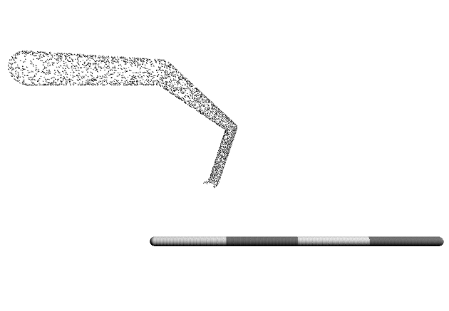
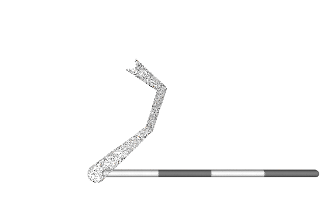
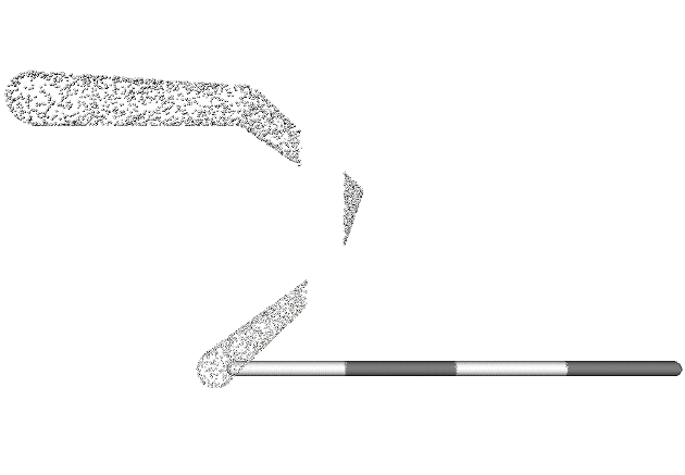
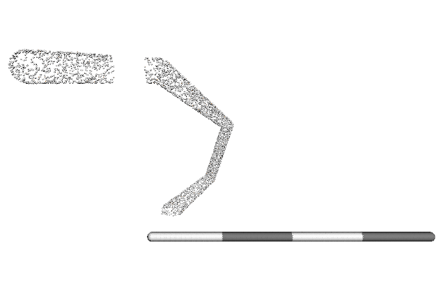
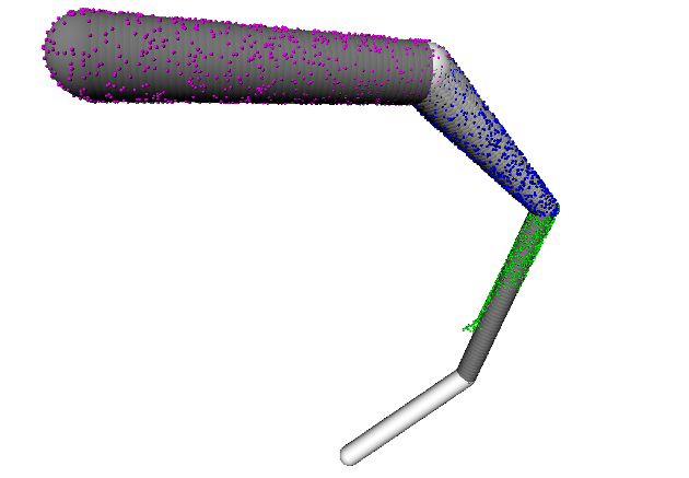
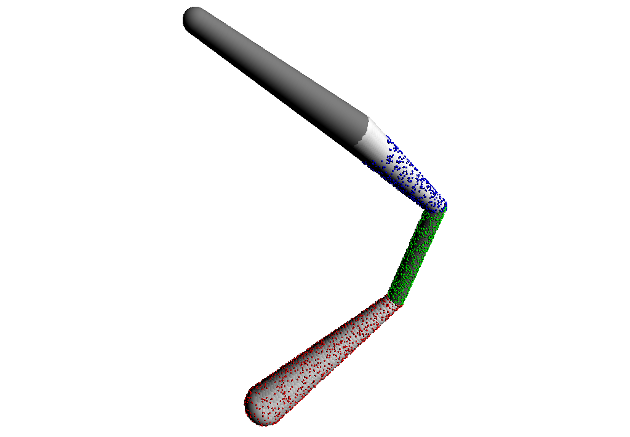
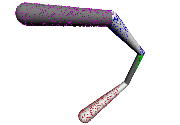
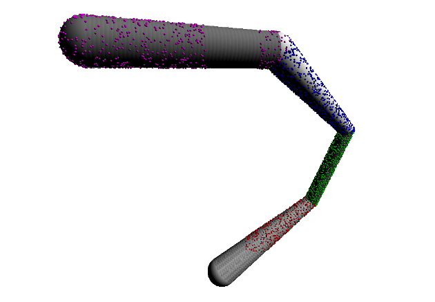
Figure 10: Evaluation of the FAKIR algorithm with respect to missing data after $20$ iterations. The first row shows the initial point set and the bottom row shows the registered bone chain.

4.2 Skeleton registration results on statues

We selected some interesting statues from various sources.

1. Dancer with Crotales, Louvre Museum

2. Dancing Faun, Pompei excavations

3. Aphrodite, Museum of Thorvaldsens

4. Old man walking, Nye Carlsberg Glyptotek

5. Esquiline Venus, Capitoline Museum

6. Old Fisherman Vatican-Louvre, Louvre Museum

7. Venus de Milo: Louvre Museum

8. Mermaid, Royal Bibliotek of Copenhagen

While the ’Dancer with crotales’ is a raw point set. The other 7 models are point sets sampled on meshes extracted from the Sketchfab website. We also use several models from the TOSCA dataset [BBK08], including nonhuman models to show the pliability of our method.

Figure 11 shows our registrations on four statues. The registration algorithm performs well for statues depicting naked characters: in this case, the registration is not hindered by additional clothing or accessories, and the simple sphere-mesh model fits well the data. Even with moderate clothing (Dancer with Crotales) FAKIR recovers the pose of the statue (see also the supplementary for more registration results). FAKIR can also work on incomplete statues on as shown in Figure 12 and on imaginary creature statues (Figure 13). We also demonstrate that FAKIR can work with real human bodies in more complex poses (Figure 14) or animals (Figure 15) from the TOSCA dataset.

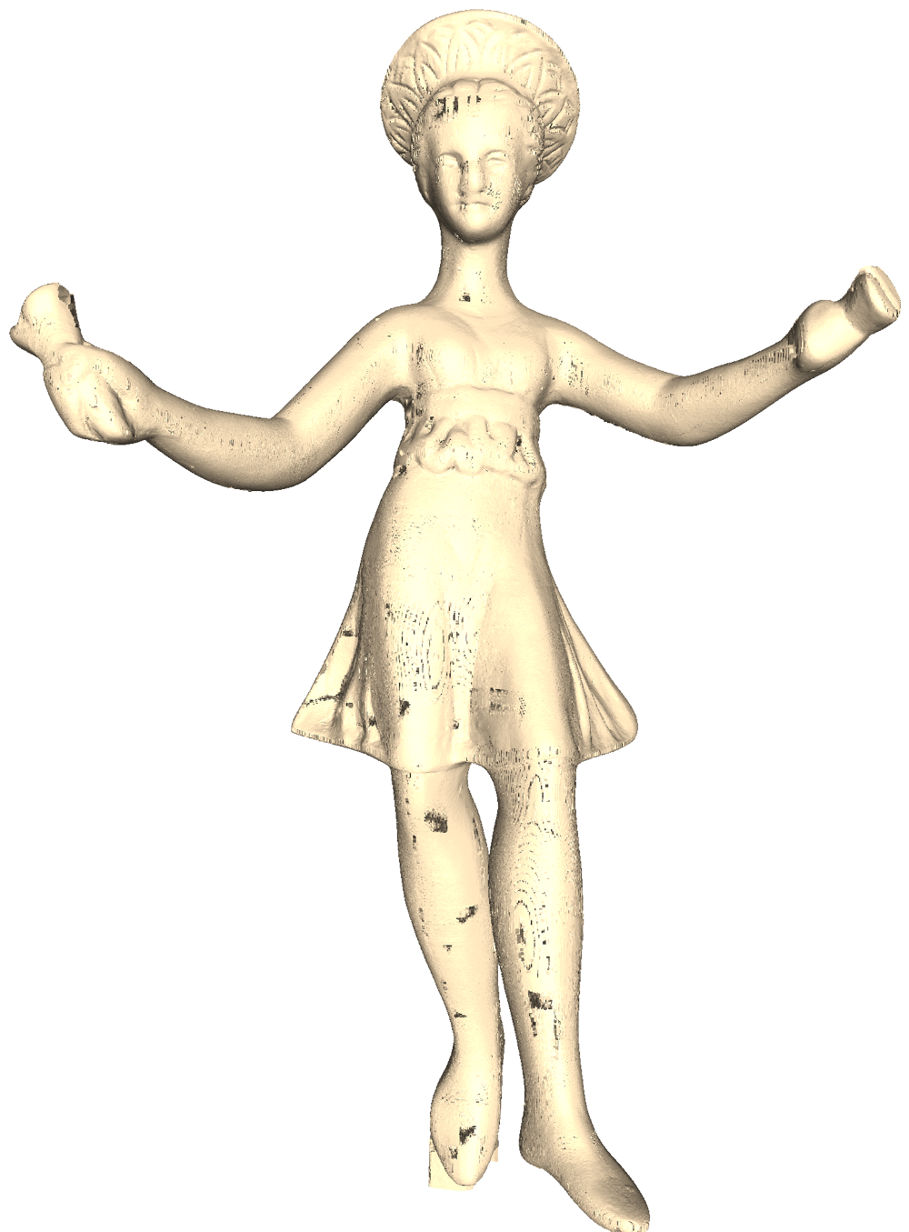
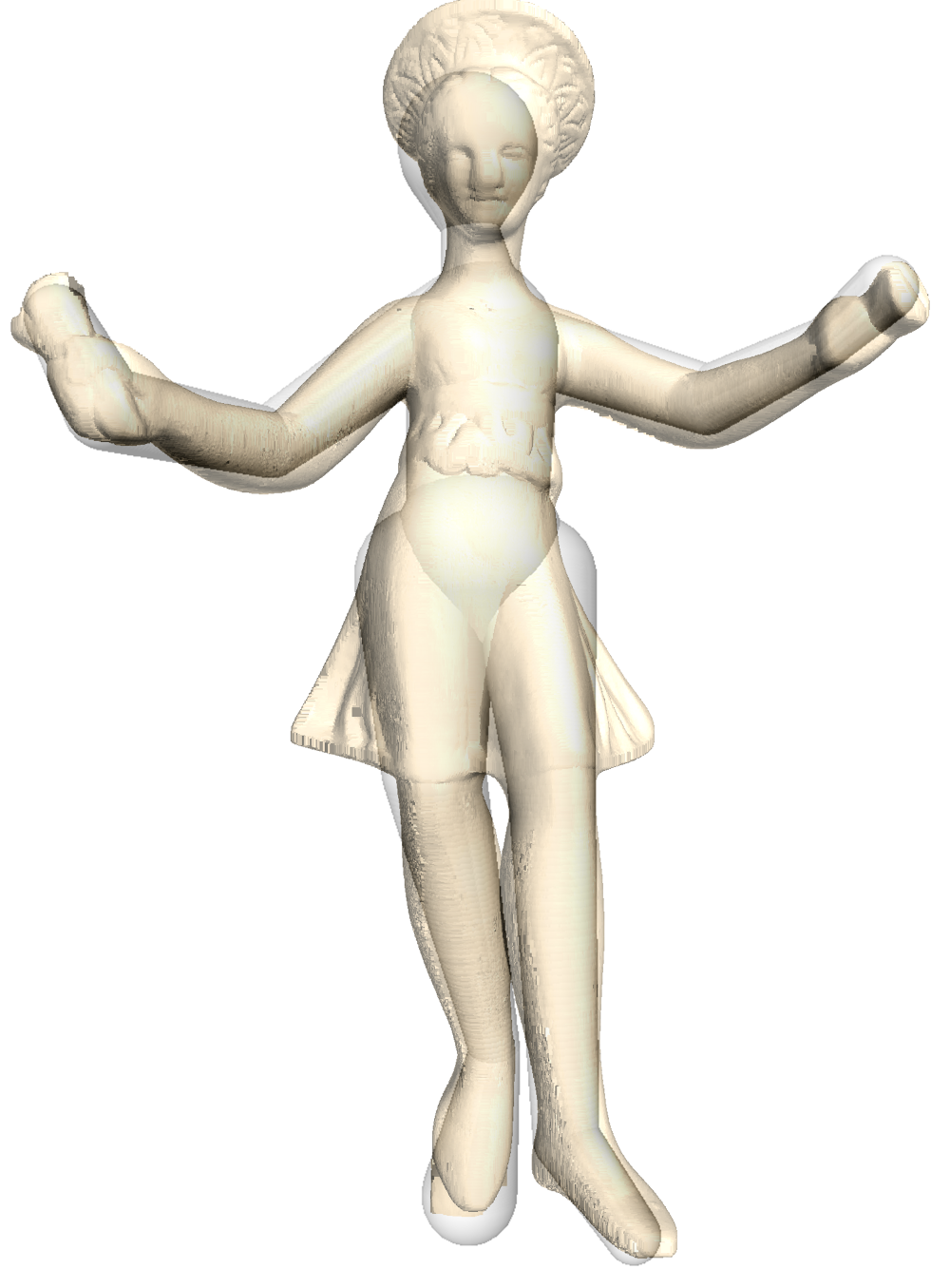
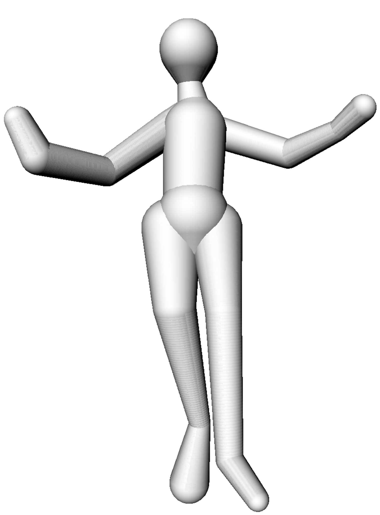
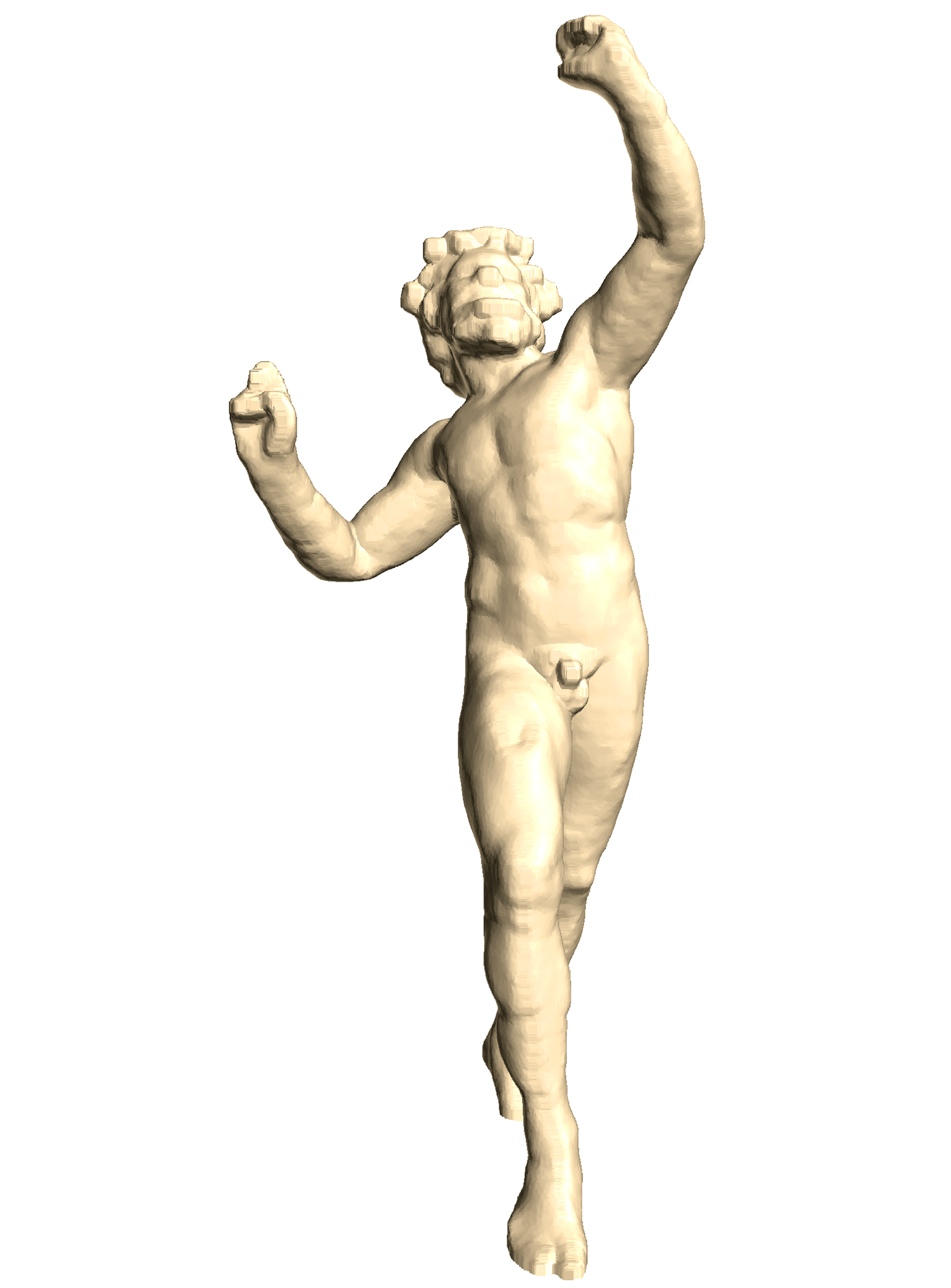
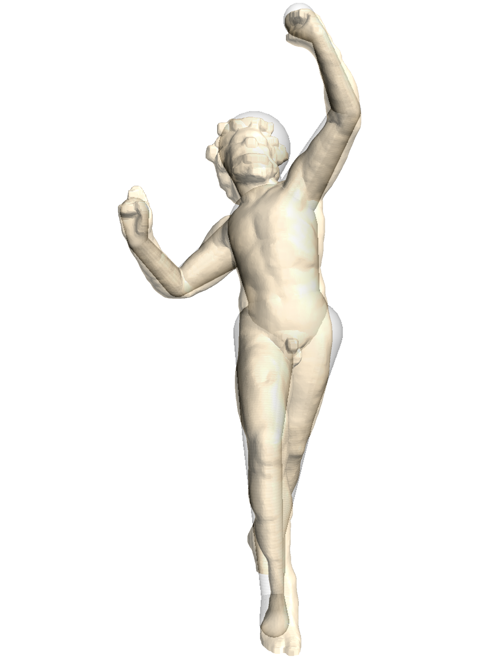
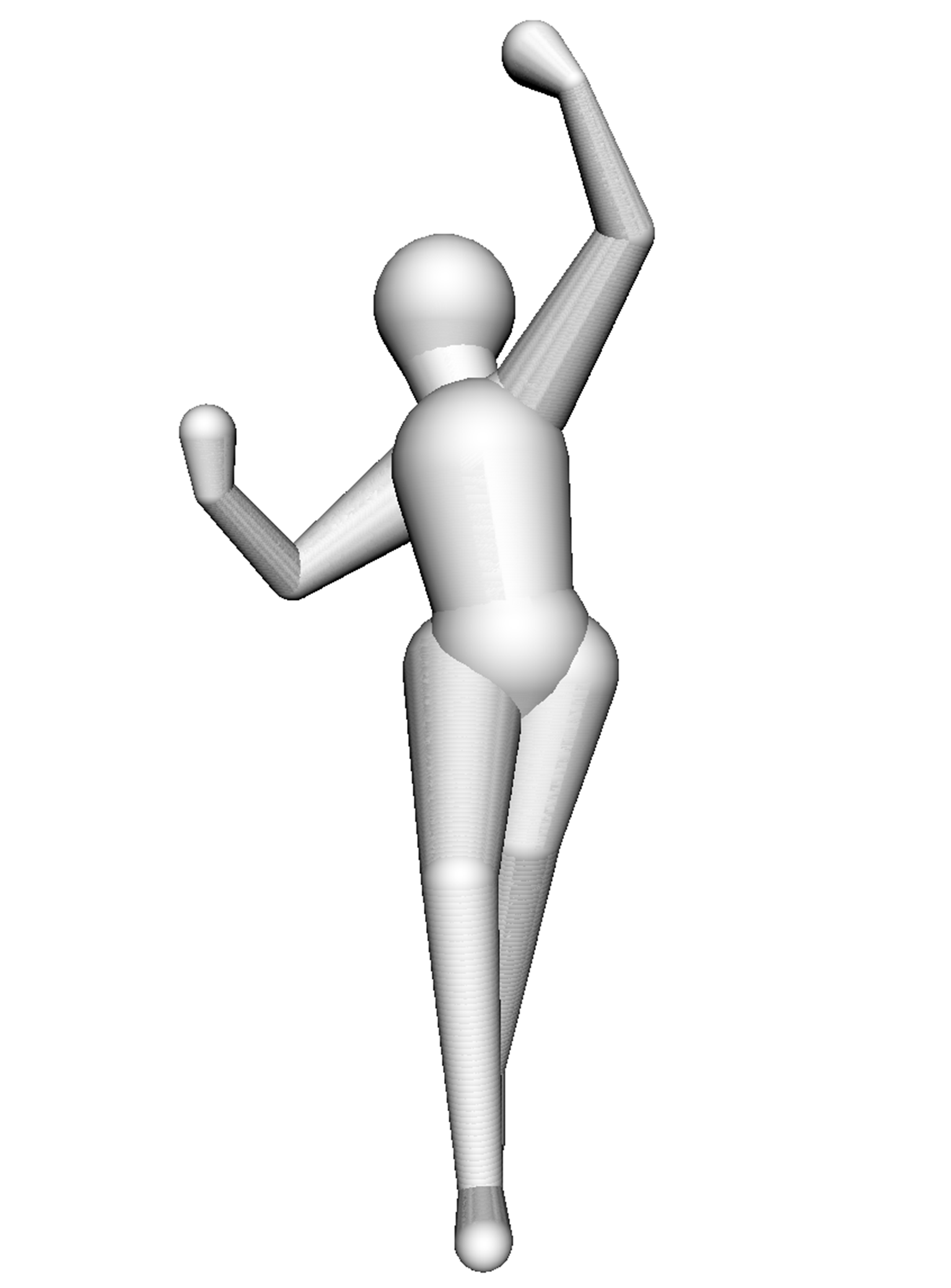
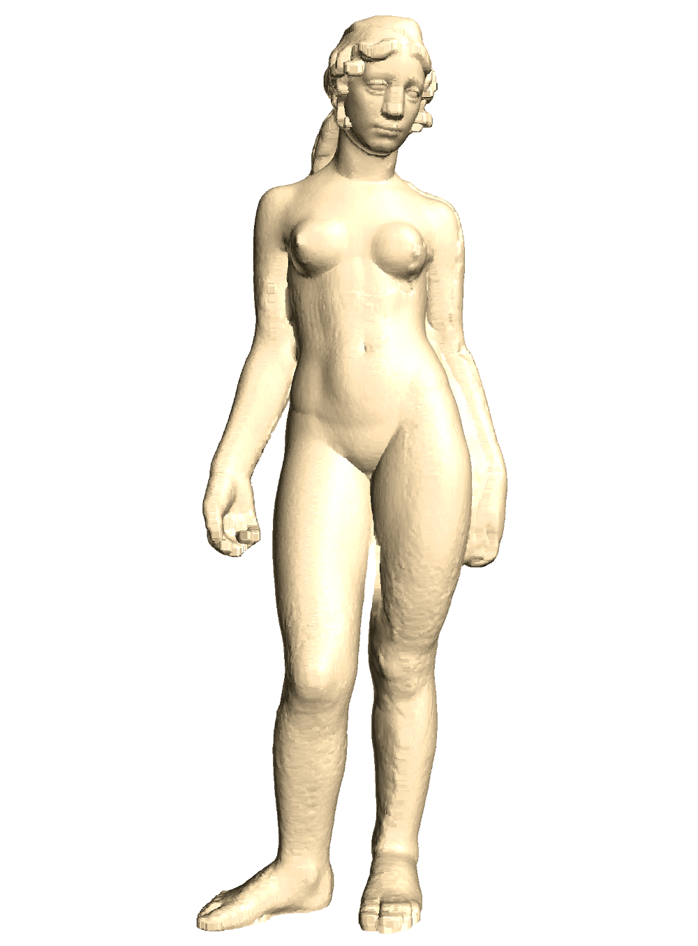
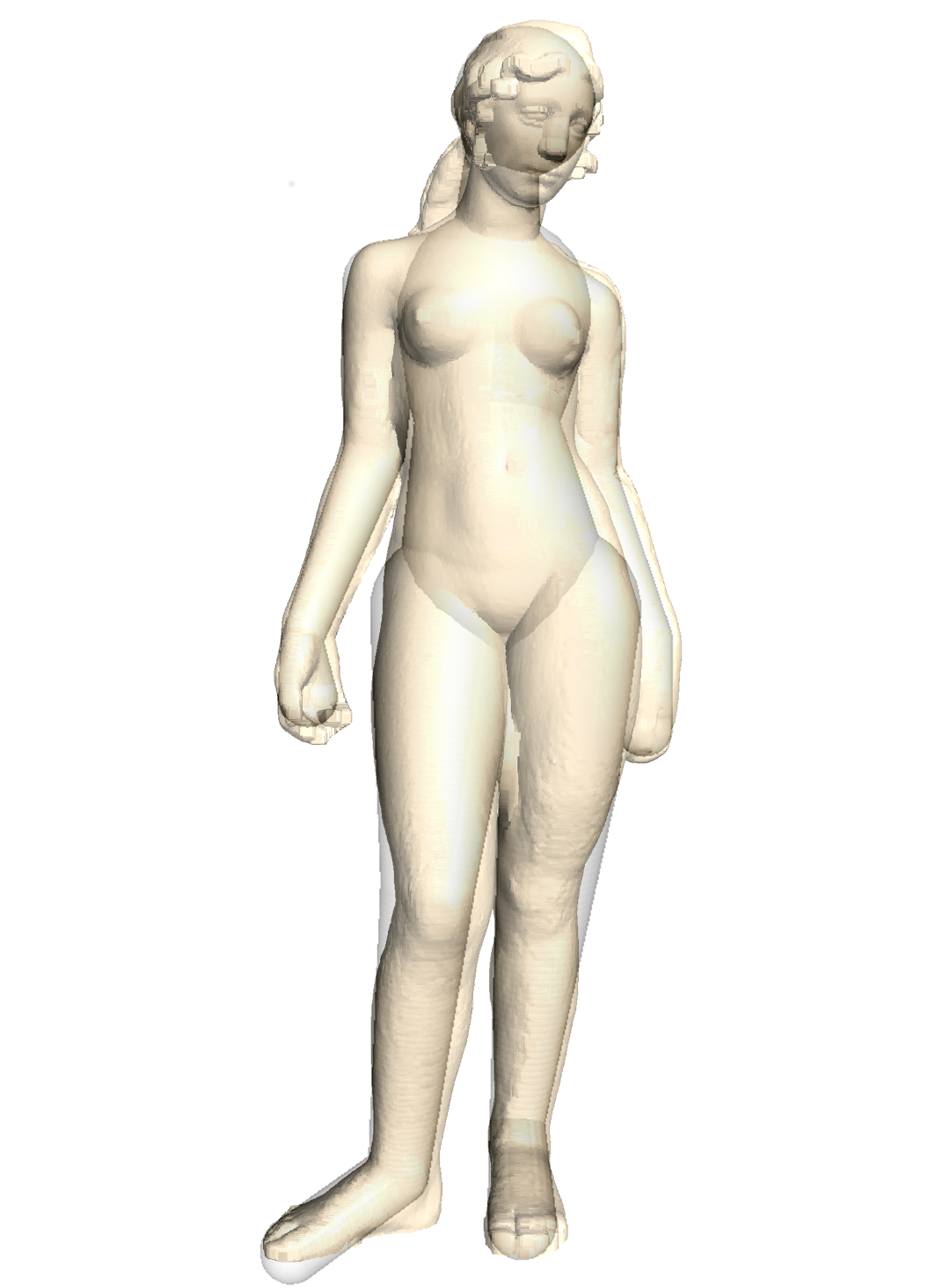
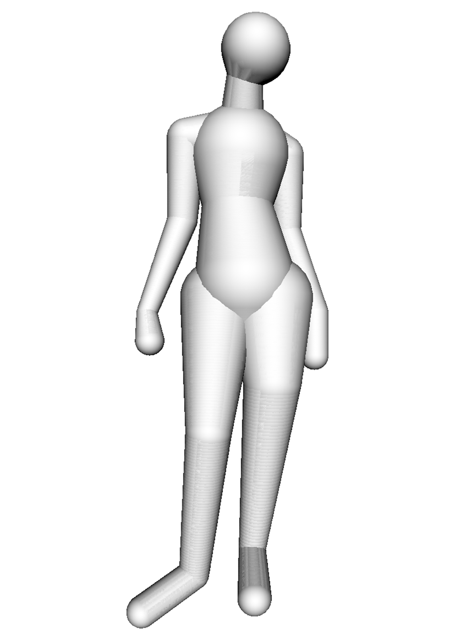
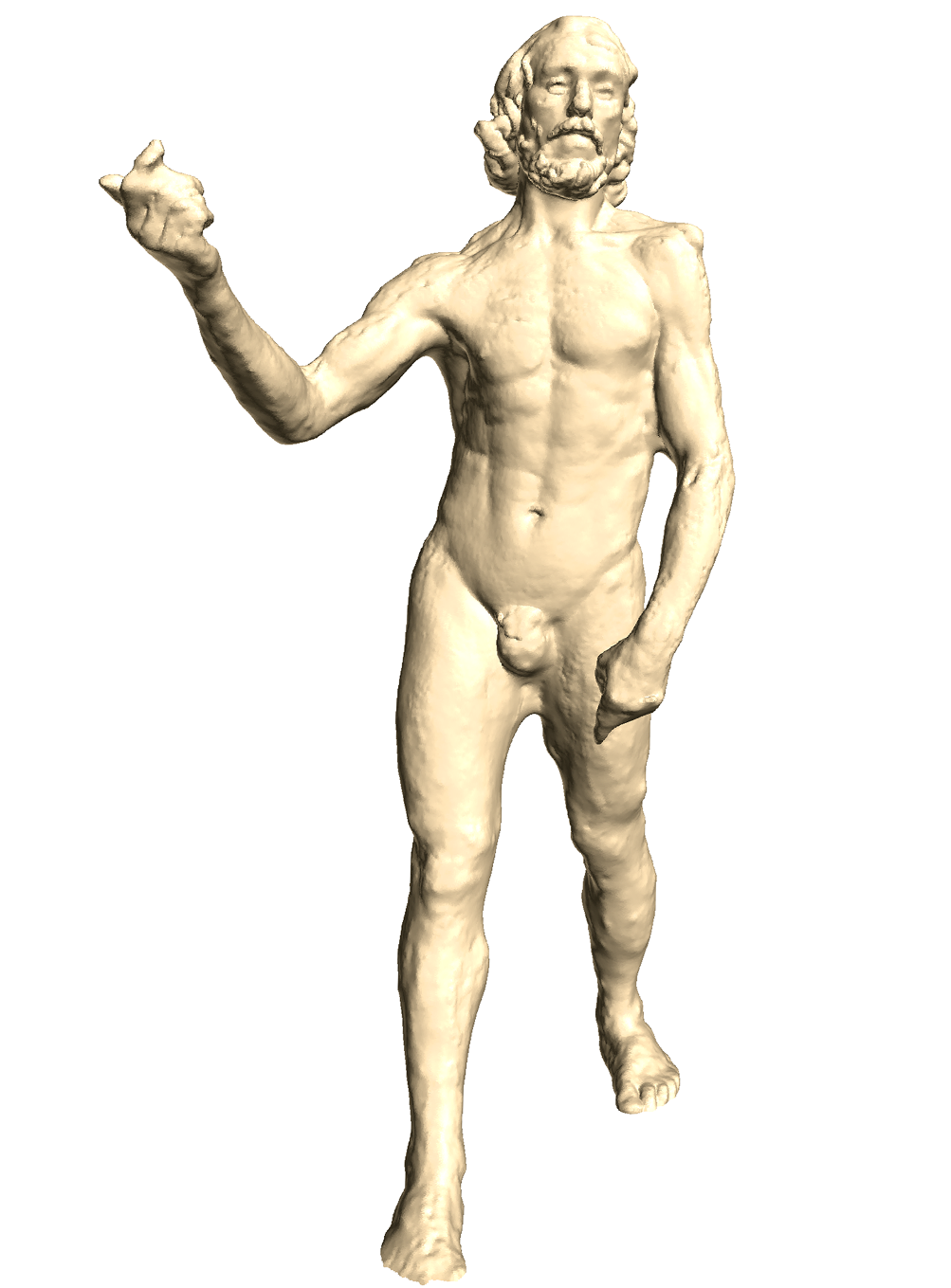
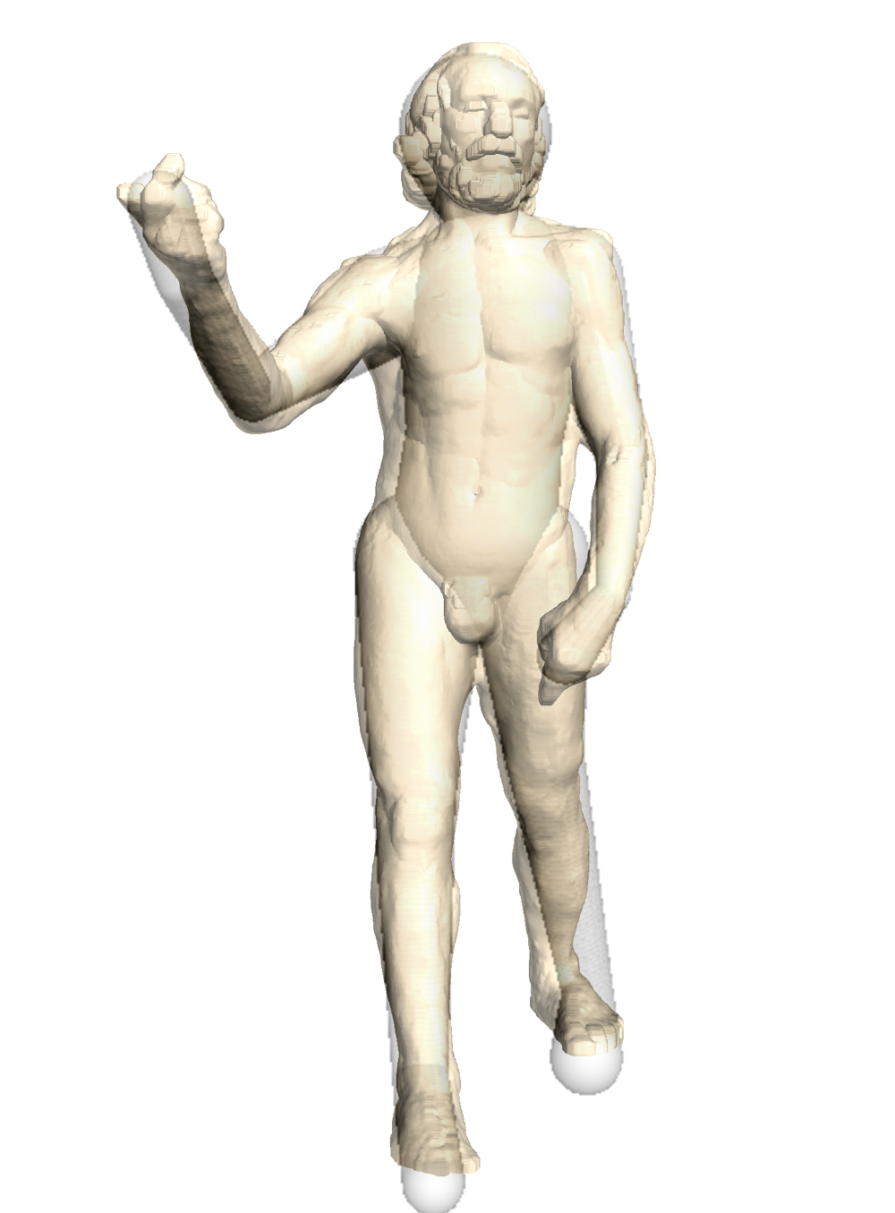
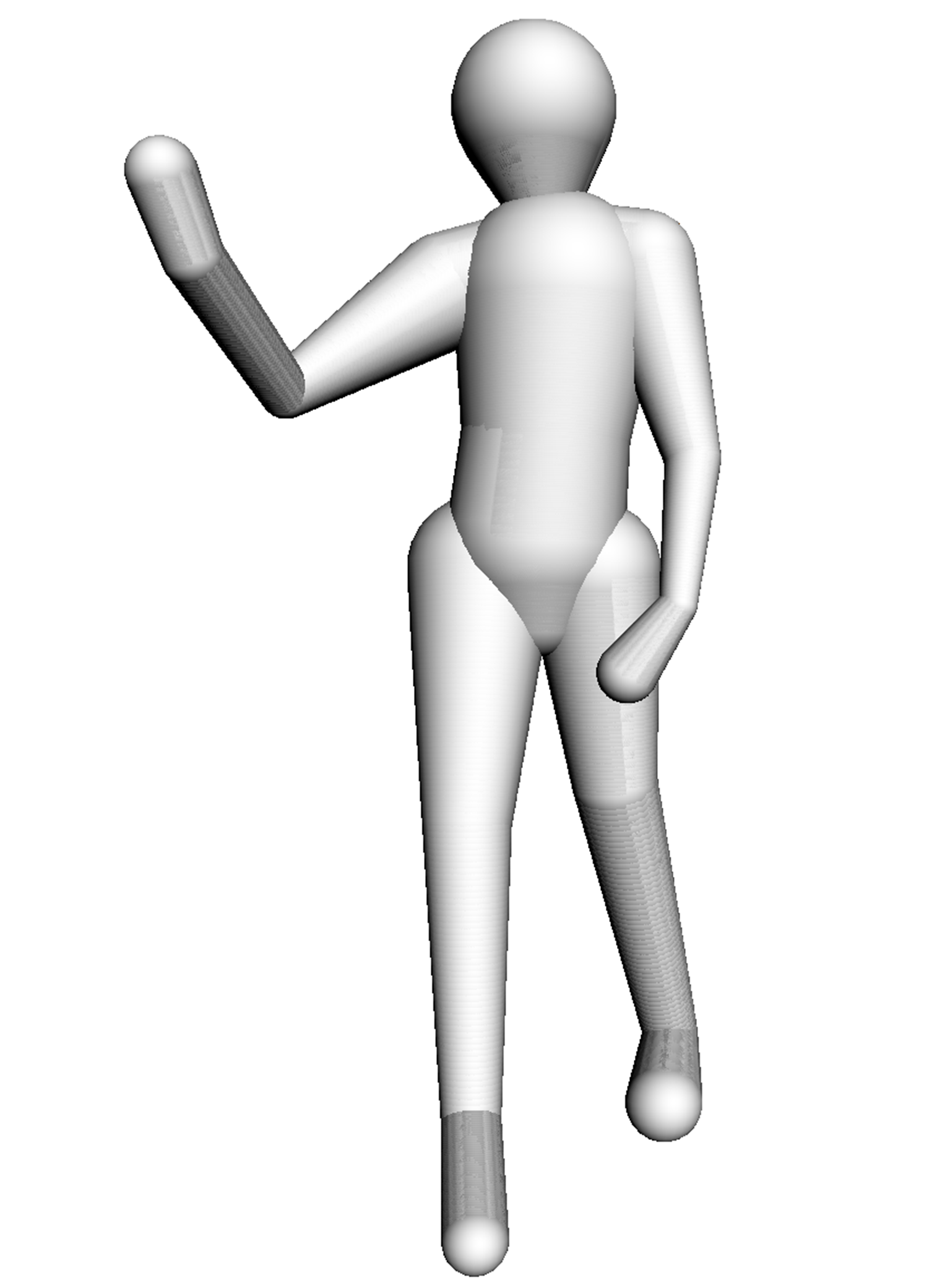
Figure 11: Registration of 4 statues: the Dancer with Crotales (first row), the Dancing Faun (second row), Aphrodite (third row) and the Old Man Walking (fourth row). First column: initial point set, second column: overlay of the registered model and the point cloud, third column: registered model.

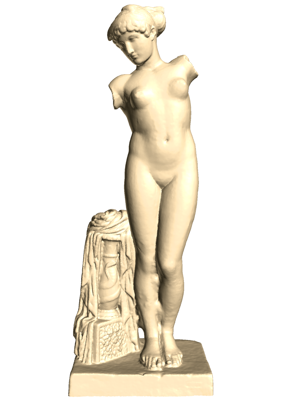
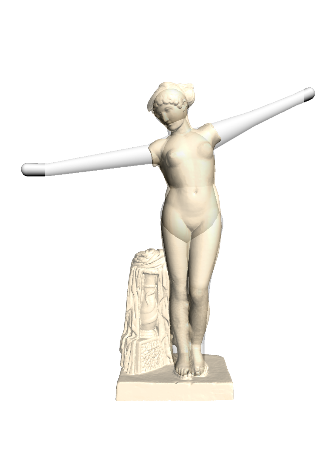
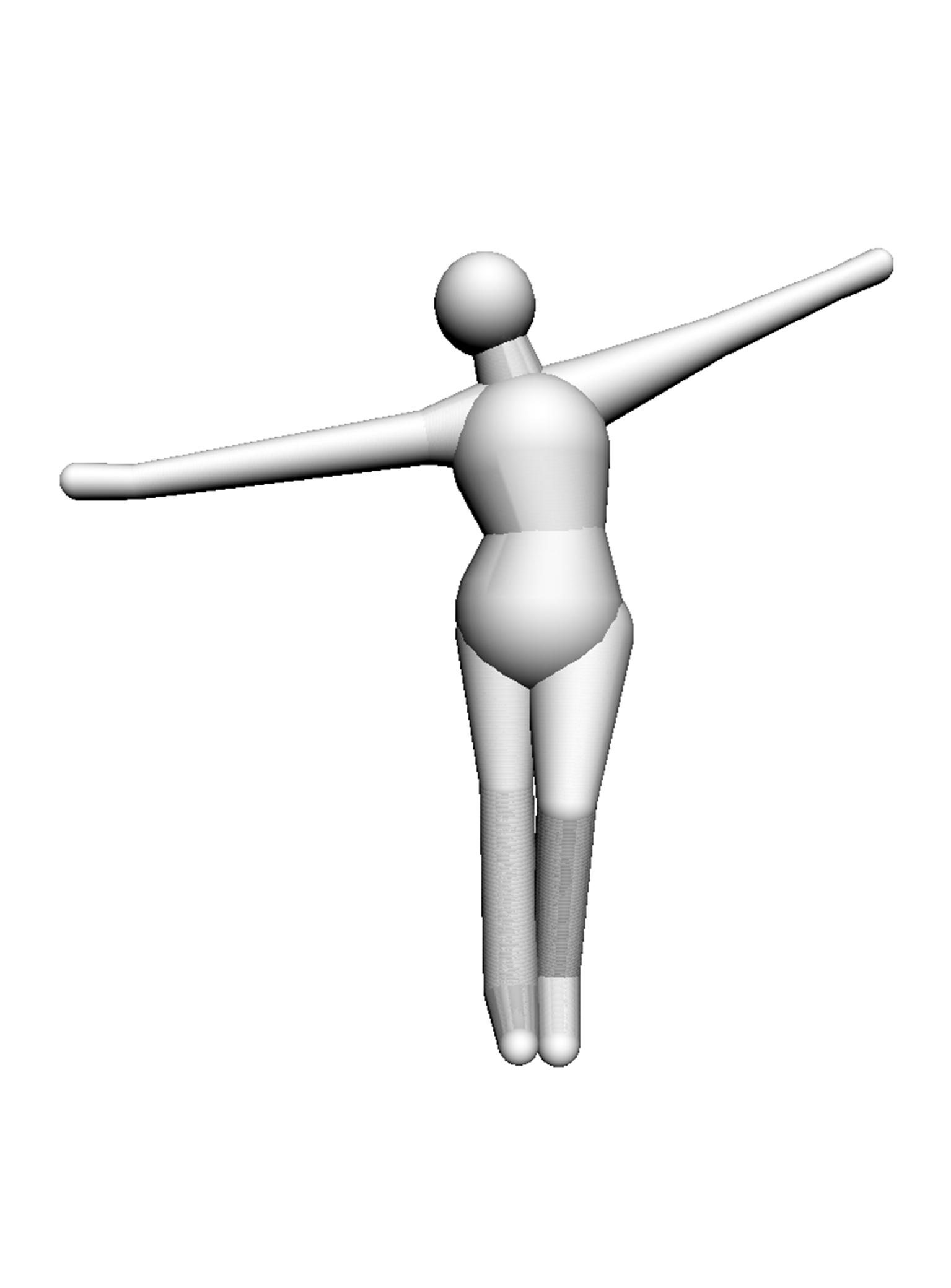
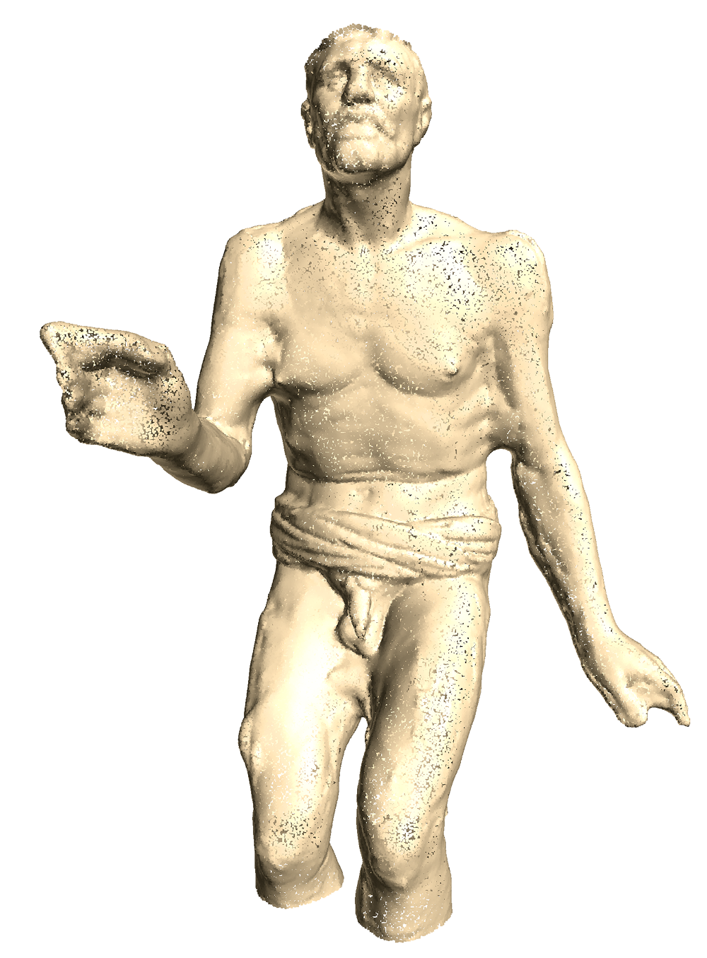
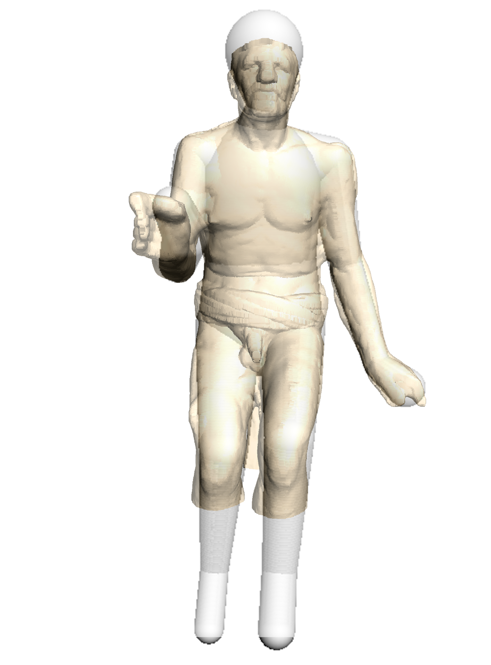
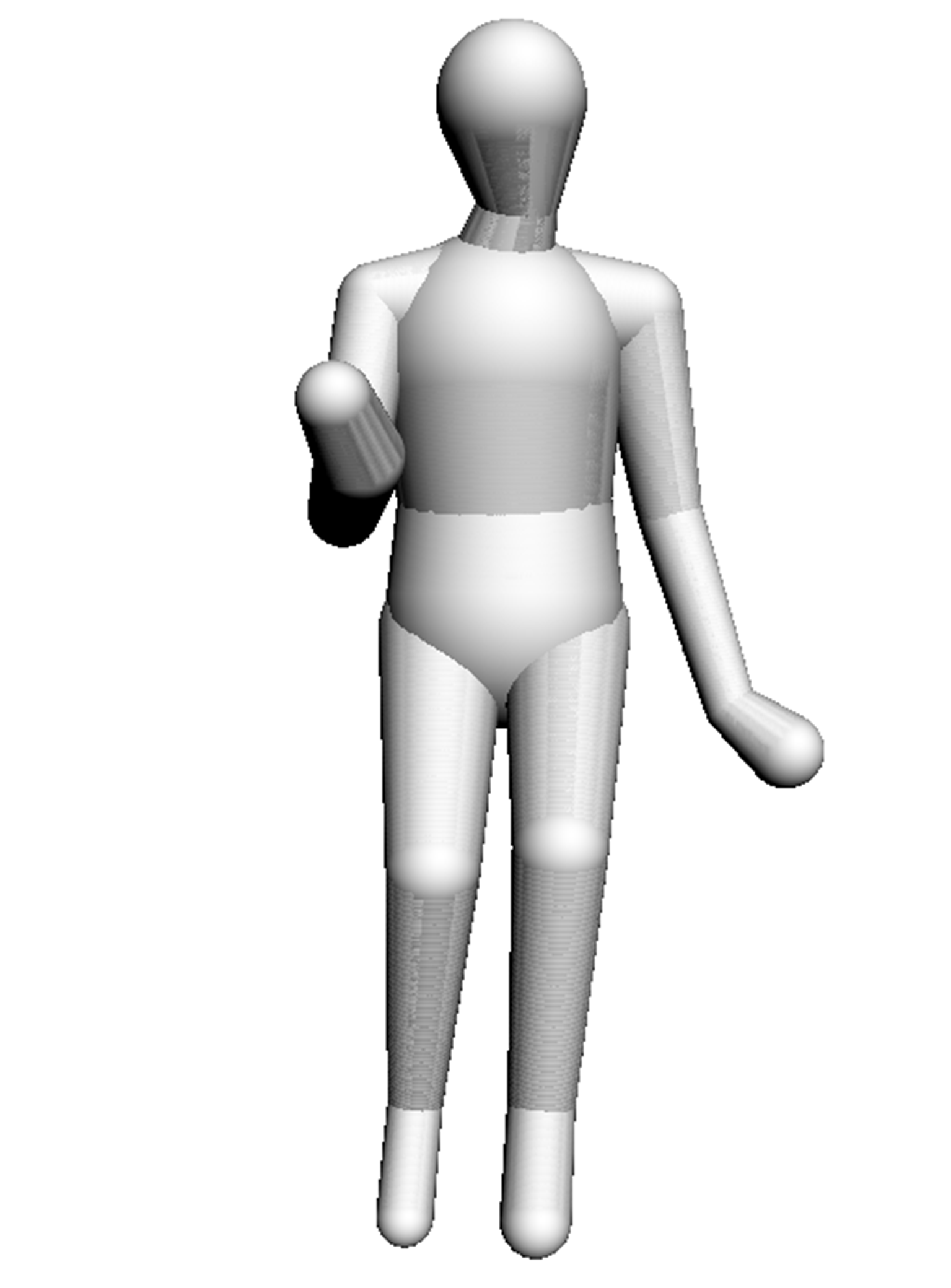
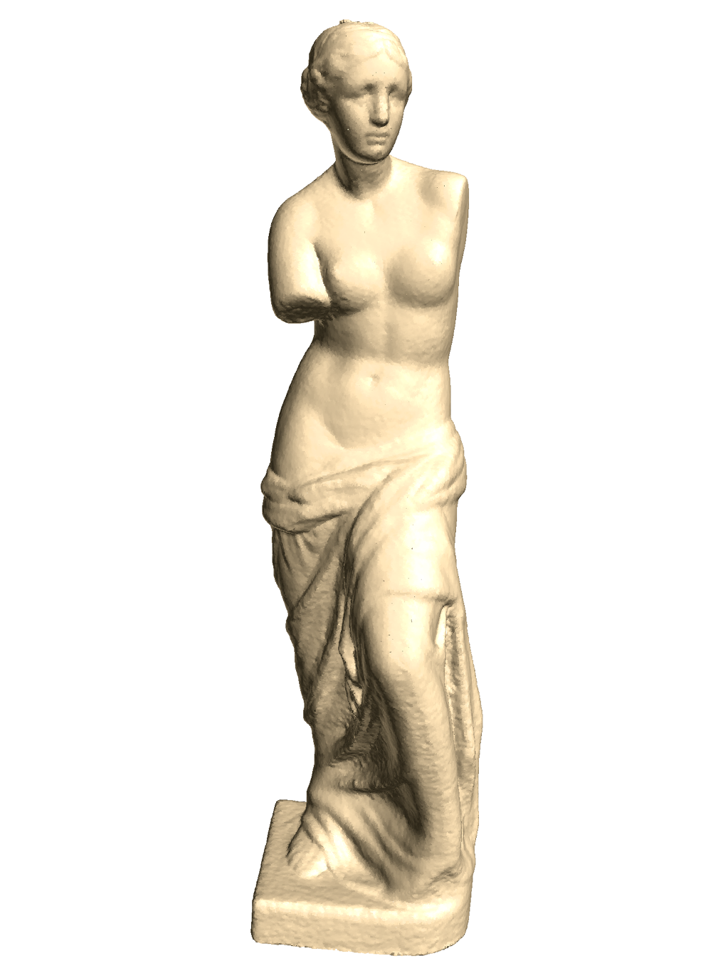
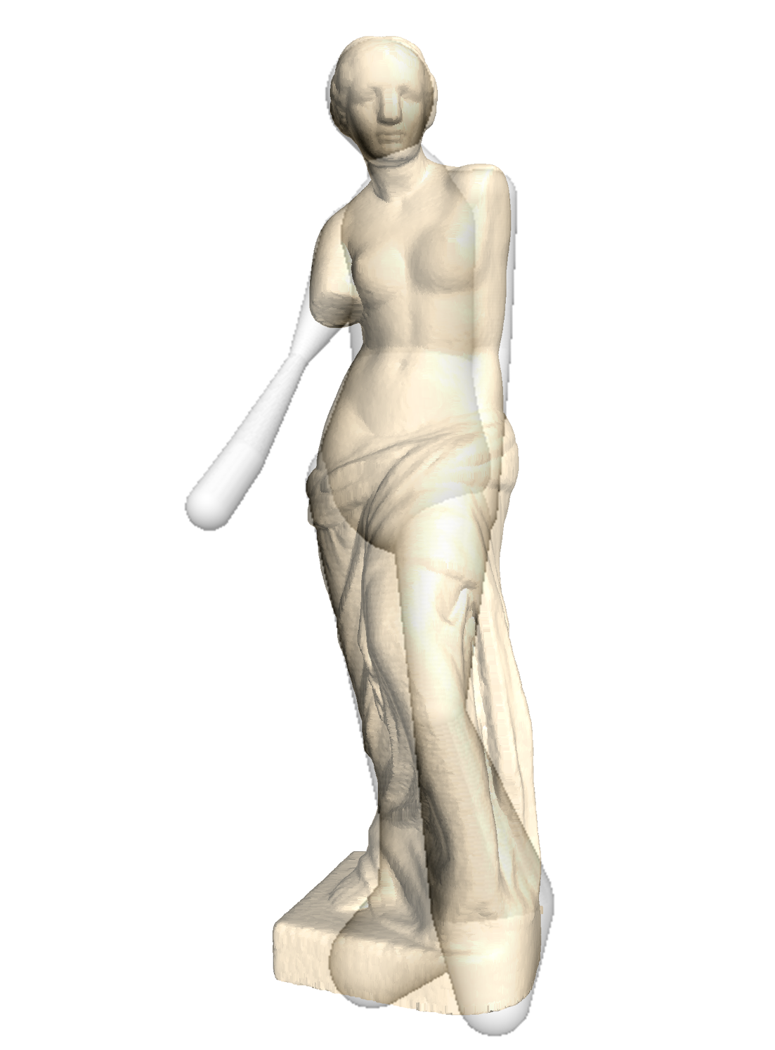
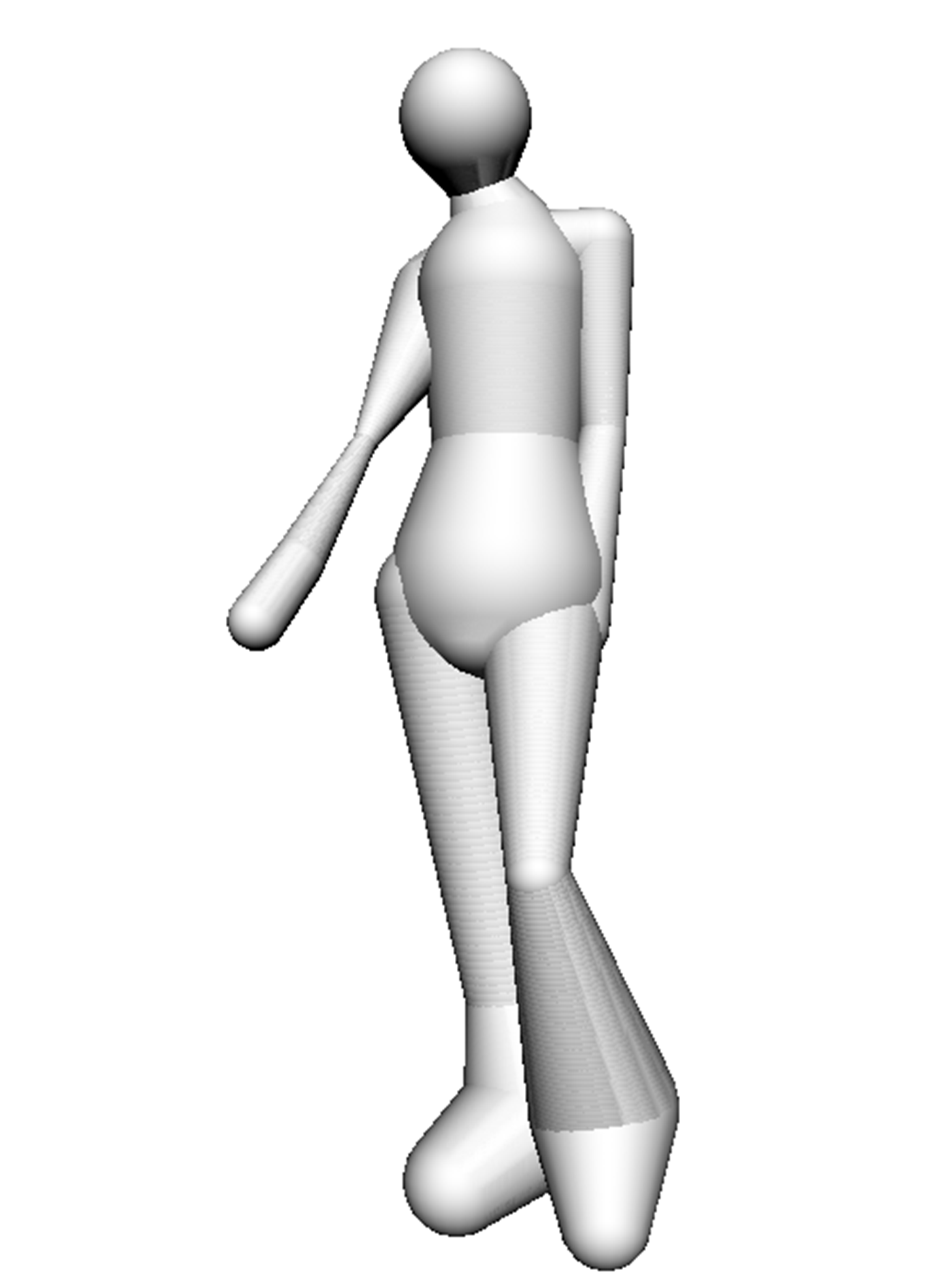
Figure 12: Registration of 3 incomplete statues, Esquiline Venus (first row), Old Fisherman (second row) and Venus de Milo (third row). First column: initial point set, second column: overlay of the registered model and the point set, third column: registered model alone.

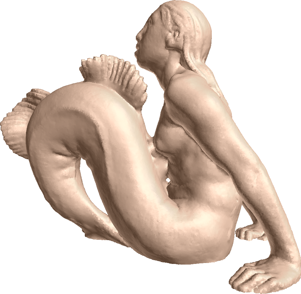
(a) Mermaid statue

(b) Overlayed registered model

(c) Registered model

Figure 13: FAKIR result on the Mermaid statue, the skeleton is a human one but with a single chain instead of two legs.

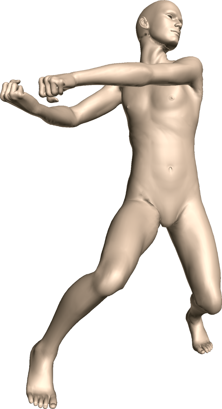
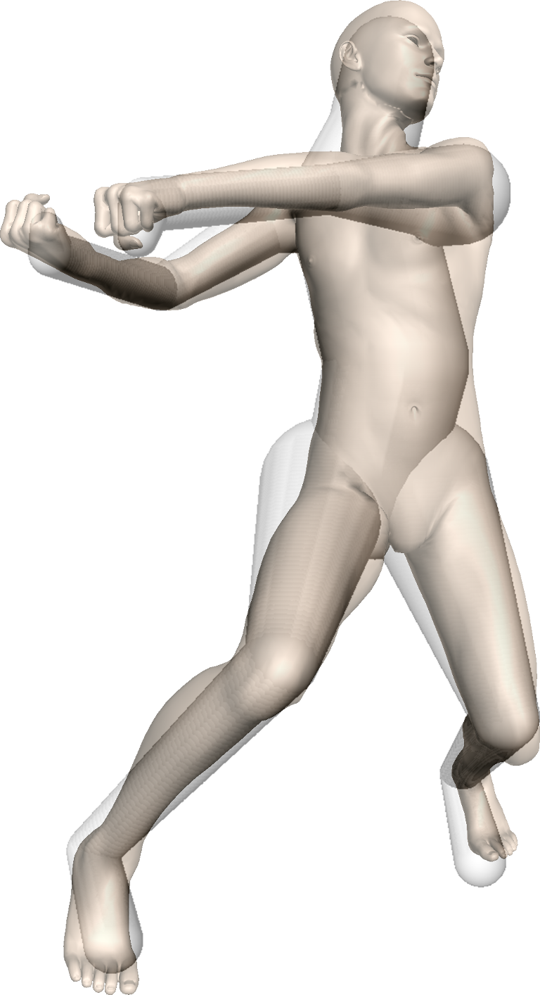
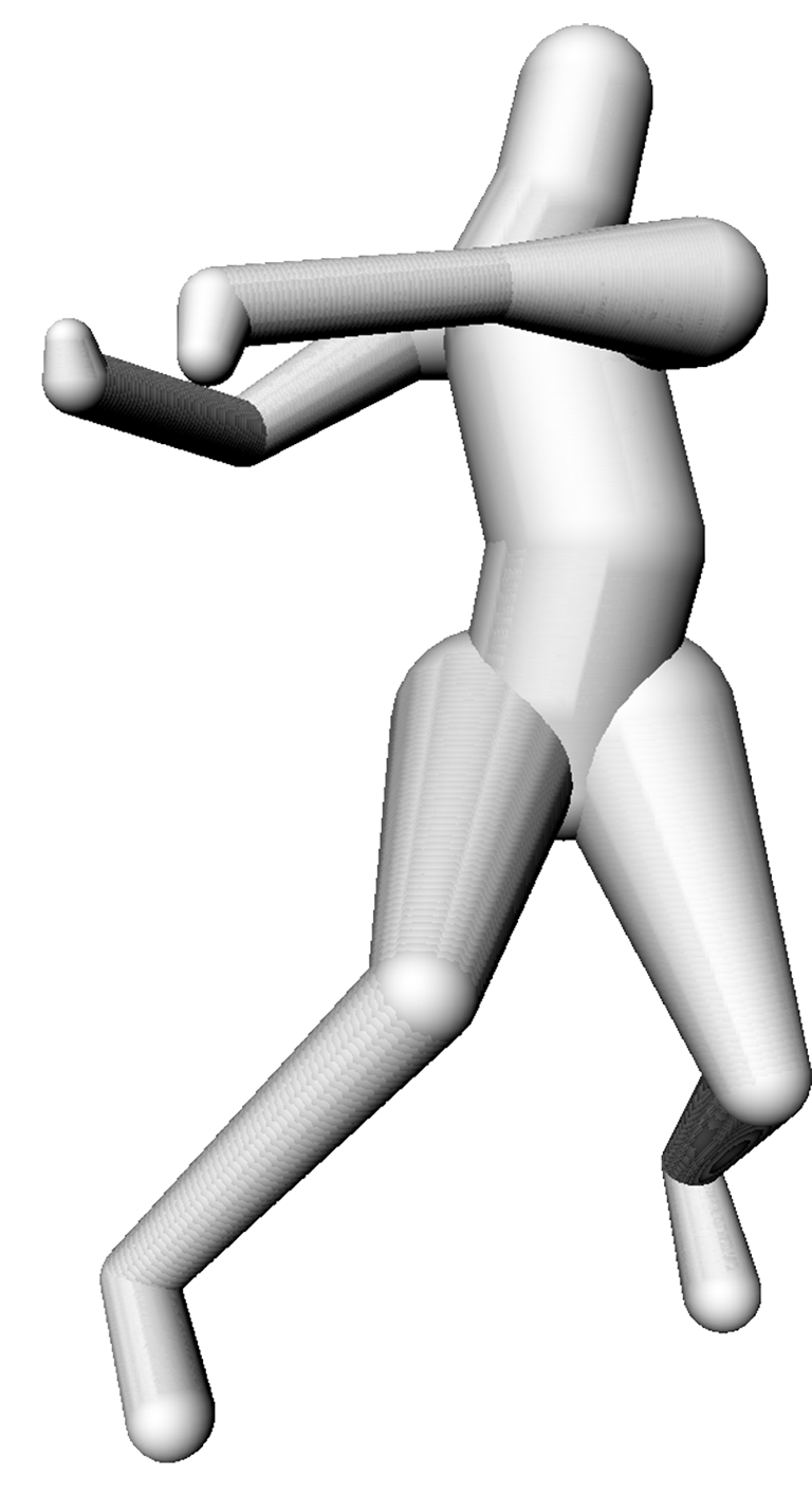
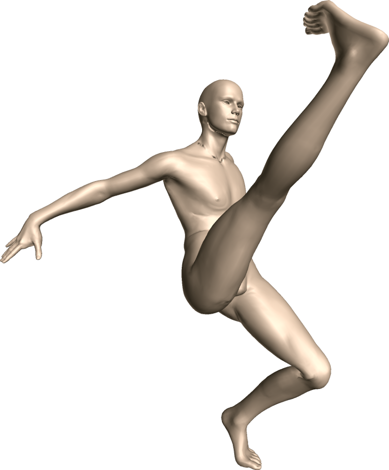
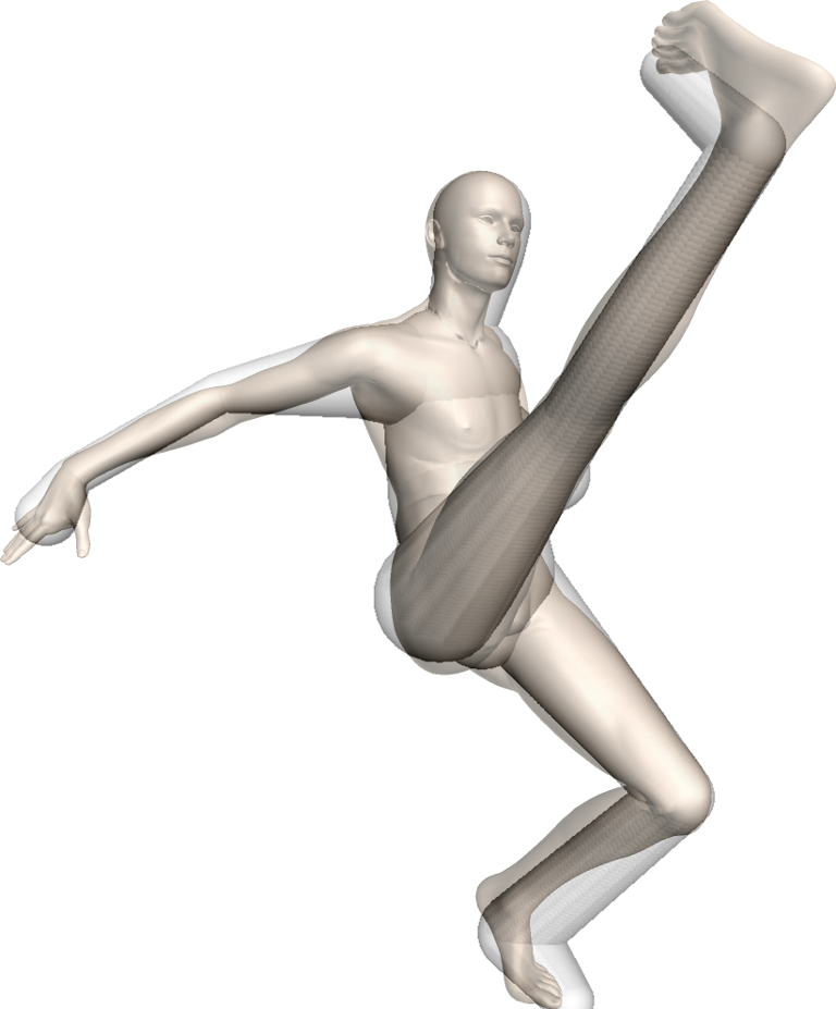
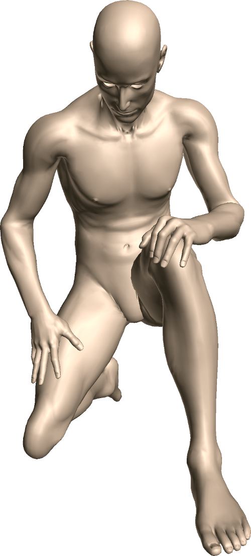
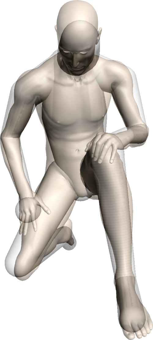
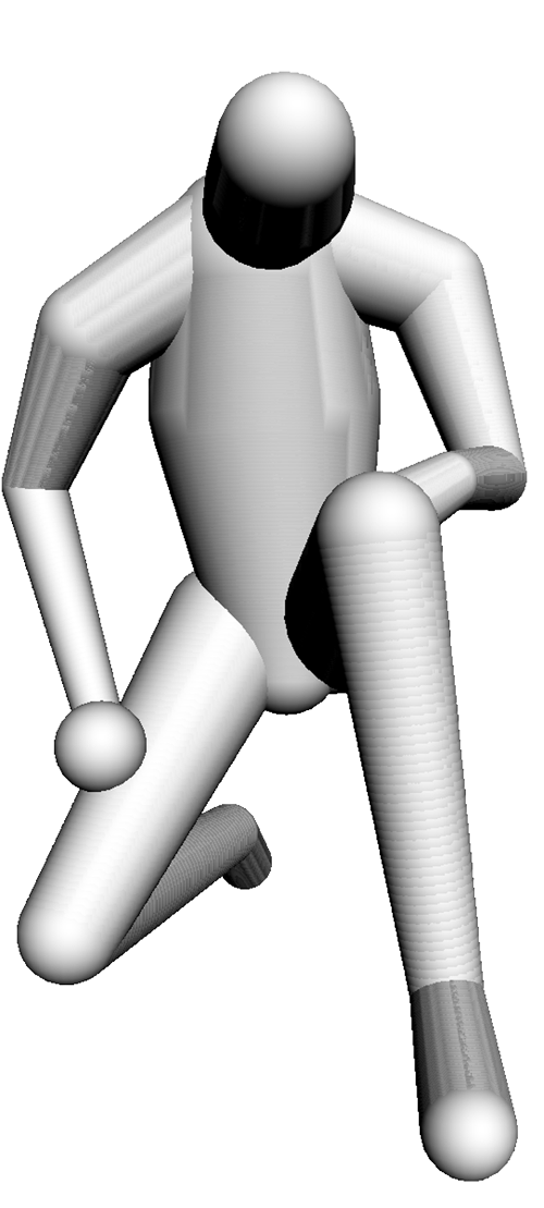
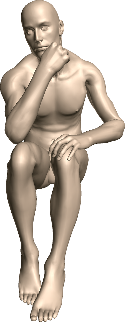
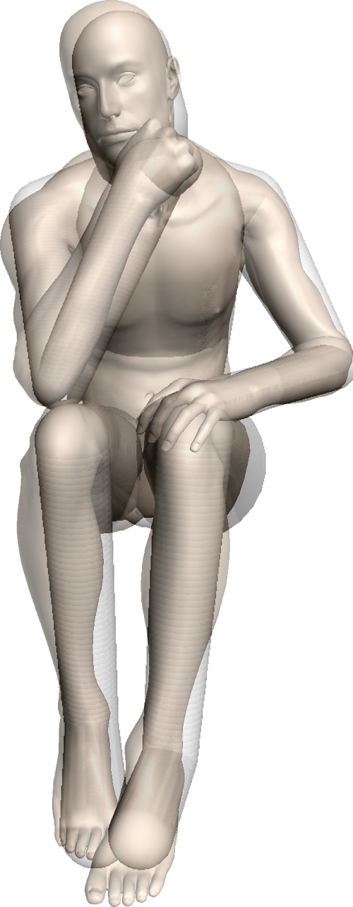
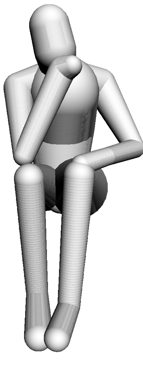
Figure 14: Skeleton registration on human in various poses from the TOSCA dataset.

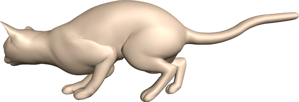
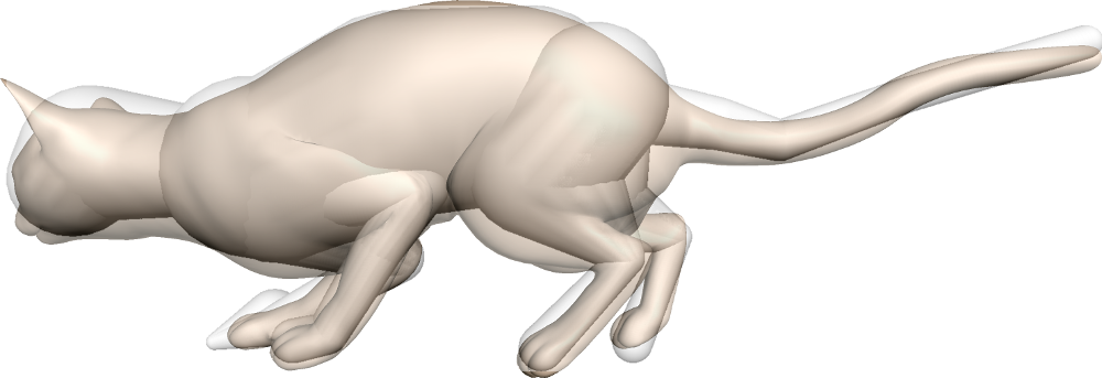
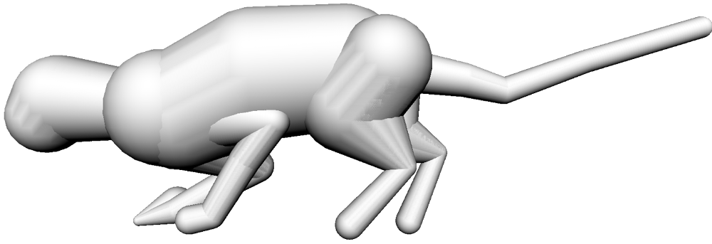
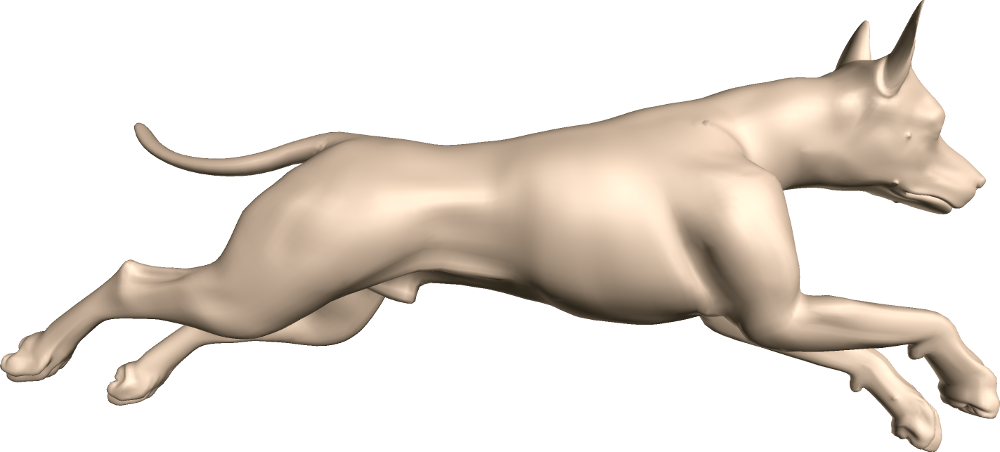
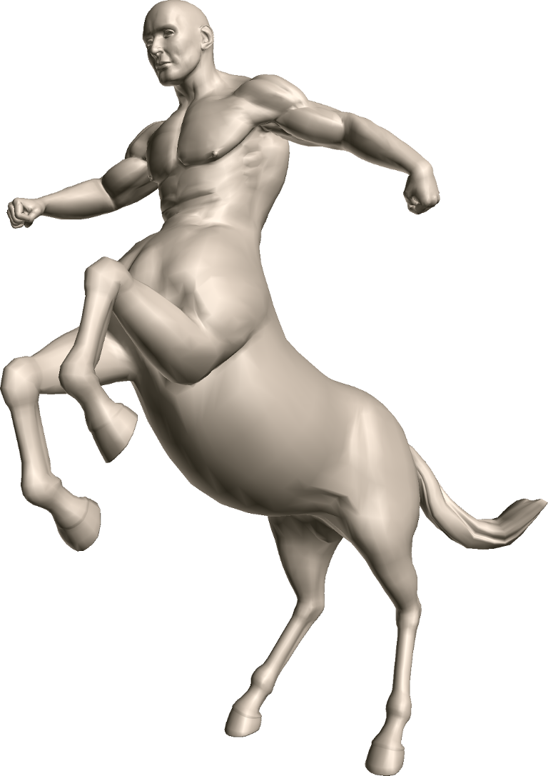
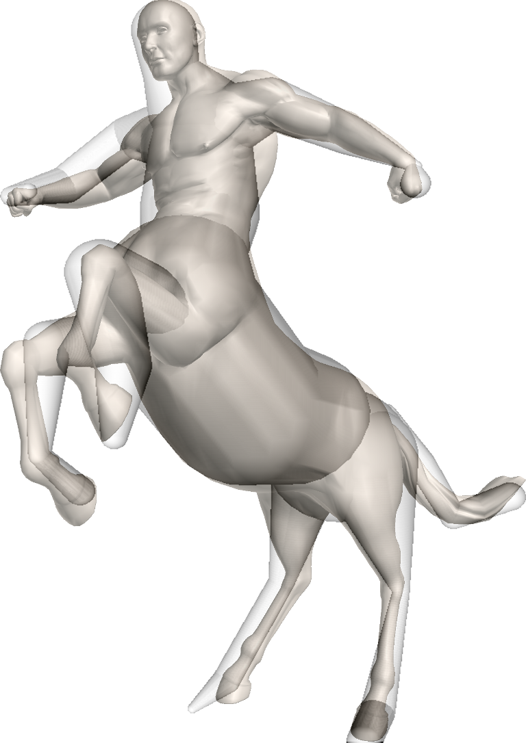
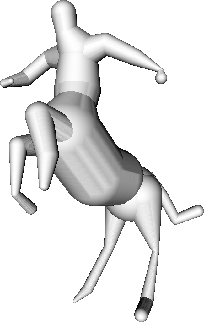
Figure 15: Skeleton registration on different animals from the TOSCA dataset. The skeleton is simply the human skeleton (Figure 2) supplemented with a bone chain for the tail.

While skeleton extraction is a much explored topic in geometry processing, we emphasize that extracting a computational geometry skeleton is very different than extracting an anatomical skeleton [HWCO^∗13, TDS^∗16]. Figure 16 show the $\ell^{1}$-medial skeleton extracted [HWCO^∗13] on the Aphrodite and Danseuse with Crotales point sets – to be compared with our results on Figures 17 and 18. This experiment shows that the geometrical skeleton definition is not enough for our purpose.

(a) Danseuse with crotales

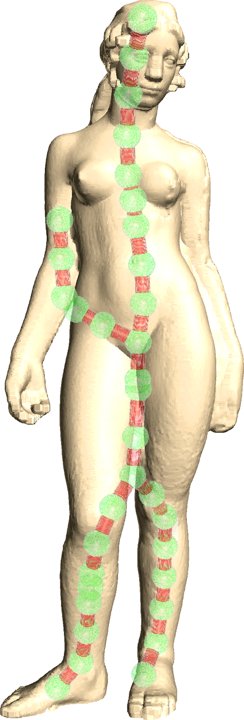
(b) Aphrodite

Figure 16: $\ell^{1}$-medial skeletons [HWCO^∗13] extracted from the Aphrodite and Danseuse with Crotales point sets. To compare to our results on Figures 17 and 18.

We compare FAKIR with Pinocchio [BP07] in Figure 17. The FAKIR algorithm yields a better skeleton registration, in particular for the shoulders and neck bones. As far as computation times are concerned, the Pinocchio method takes about $35s$ for a mesh with $138048$ vertices, which is roughly the same time as the $10$ iterations of FAKIR optimizing not only for the joint positions but also for the bone radii (38s). Furthermore, a single iteration of FAKIR takes 9s and already provides a better result with a much more plausible shoulders location. However it is important to note that the Pinocchio method does not require an initial skeleton position, while our method requires one of the joint to be not far from its optimal position (in this experiment we chose the pelvis joint).

(a) Pinocchio (vanilla)

(b) Pinocchio (our skeleton)

(c) FAKIR (1 iteration)

(d) FAKIR (10 iterations)

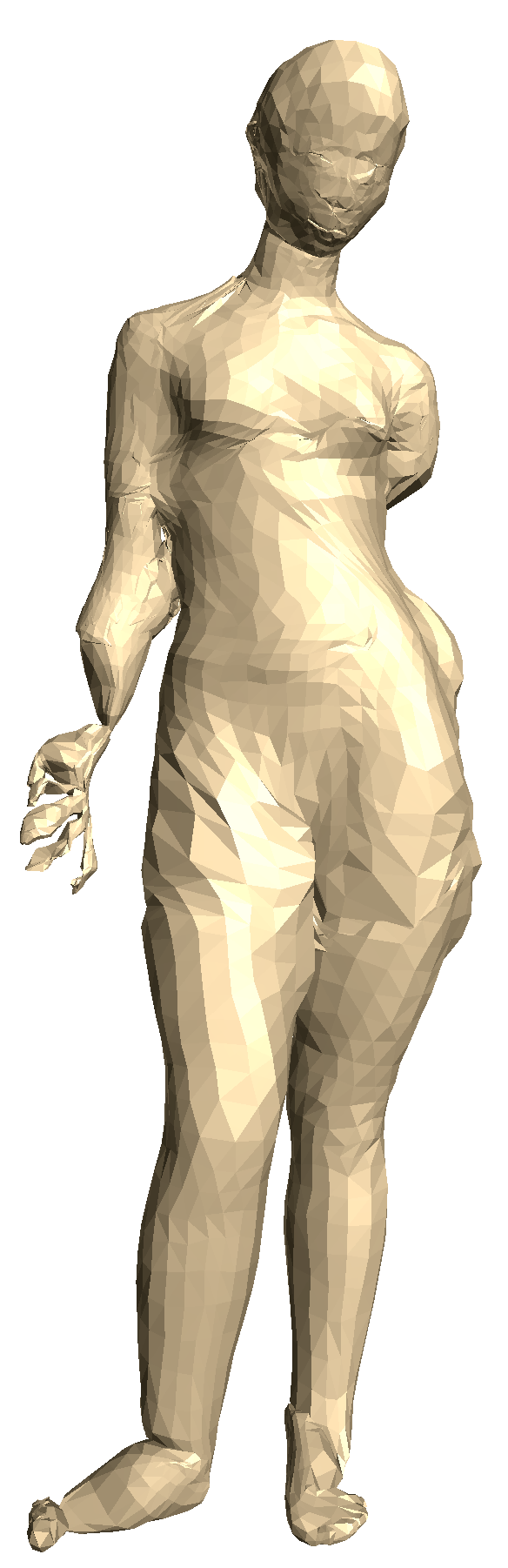
(e) FARM

Figure 17: Comparison with Pinocchio [BP07] and FARM [MMRC20] algorithm on the Aphrodite statue. From left to right: (a) Pinocchio with the Pinocchio-provided initial skeleton (17 bones); (b) Pinocchio with our initial skeleton (22 bones); (c) FAKIR with our initial skeleton after a single forward iteration; (d) FAKIR with our initial skeleton in 10 iterations. Only the skeleton is displayed since the bone radii are not taken into account by Pinocchio. (e) Model reconstructed by the FARM method.

We also compare compare FAKIR with the SMPLify method [BBLR15] (Figure 18). First we compute a front-view rendering of the shape and run DeepCut [PIT^∗16] to estimate the joint position used for SMPLify. The registration is clearly less accurate than ours (Figure 18b). We then extend SMPLify method to multi-view images using epipolar constraints to estimate a 3D joint positions from 2D joint positions obtained by DeepCut before applying SMPLify, which slightly improves the registration (Figure 18c). We also show that our articulated model regression can serve to initialize an SMPL model, leading to a better registration than with DeepCut (Figure 18d). However, the shape estimation of SMPL still cannot fit a statue with non-realistic body proportions.

Finally we compare FAKIR with the FARM method [MMRC20] a fully automatic method for registering an underlying model, such as SMPL, to a point set or a mesh. While this method exhibits excellent results on humanoid shapes, in the case of artistic statues, with irrealistic body proportions (Figure 17) or with moderate garments (Figure 18), it cannot reconstruct a plausible model. Furthermore, scanned statues often exhibit inconsistent topologies, such as an arm glued to the body (Figure 17) which is not handled by the FARM method.

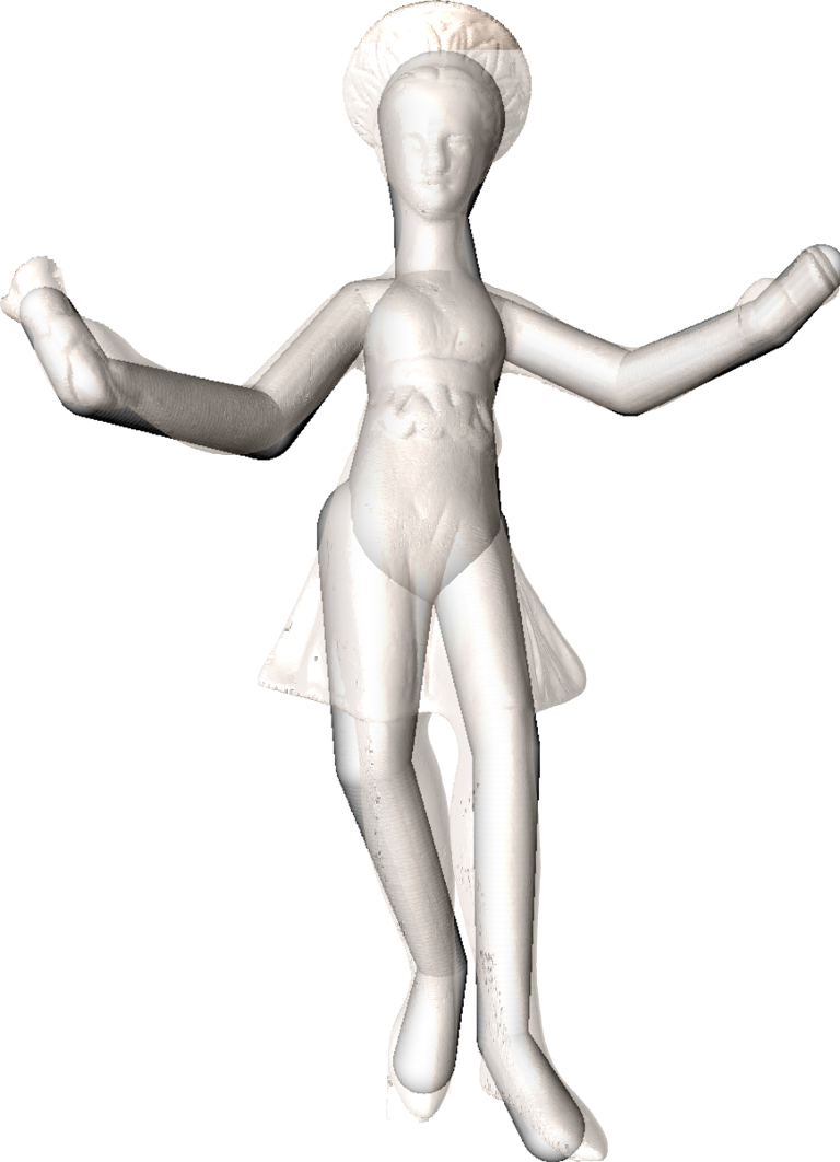
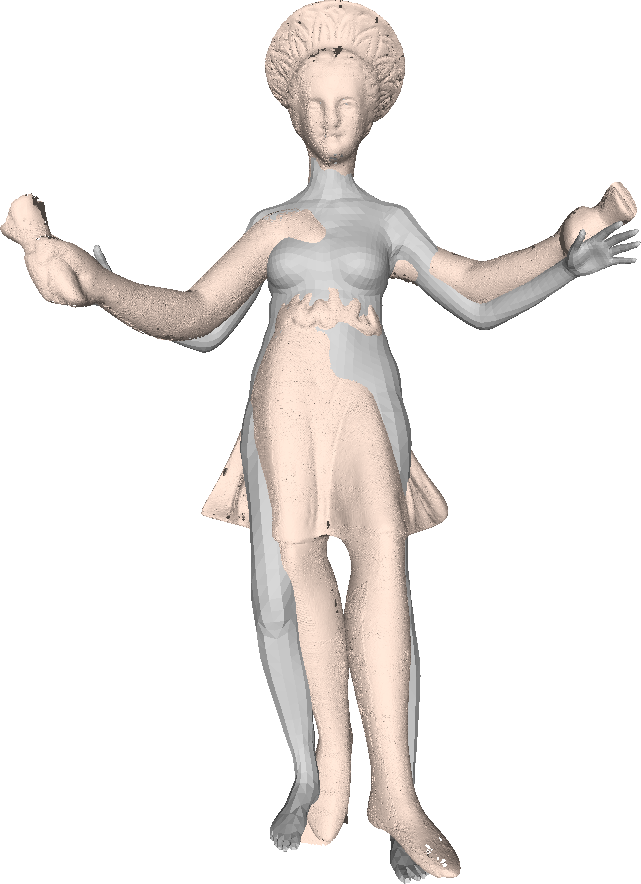
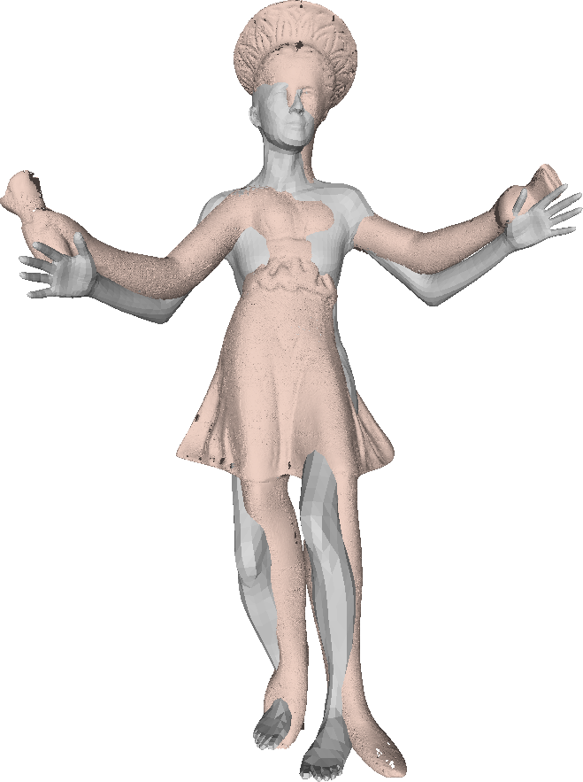
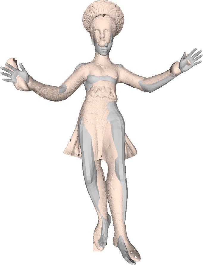
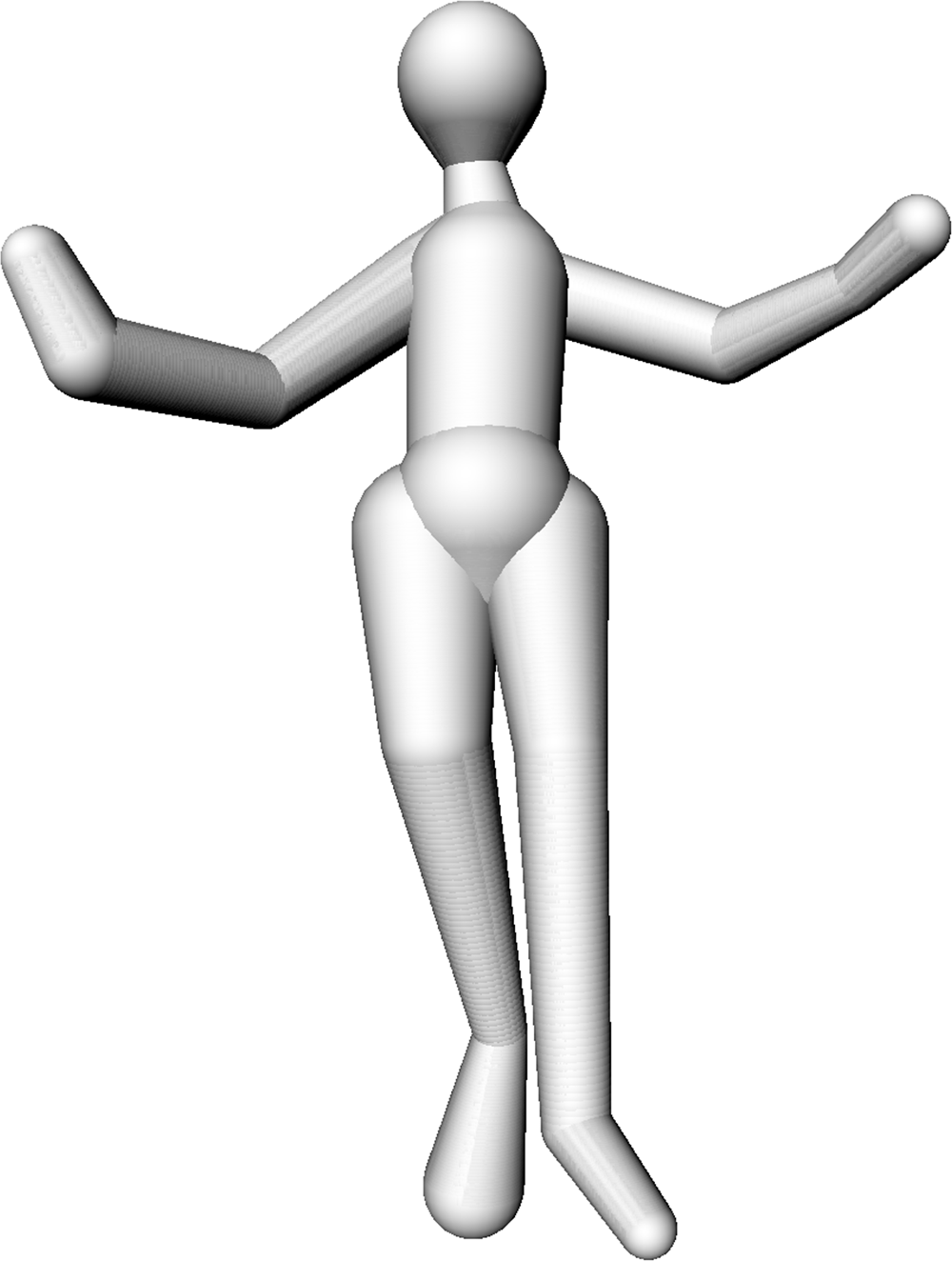
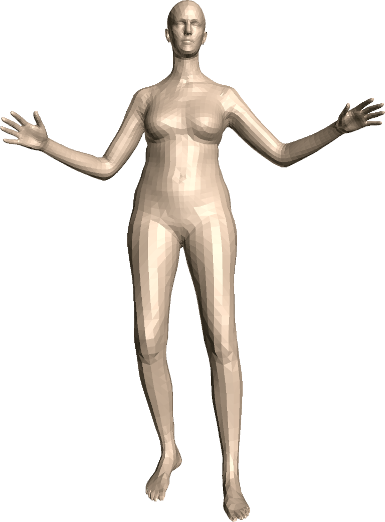
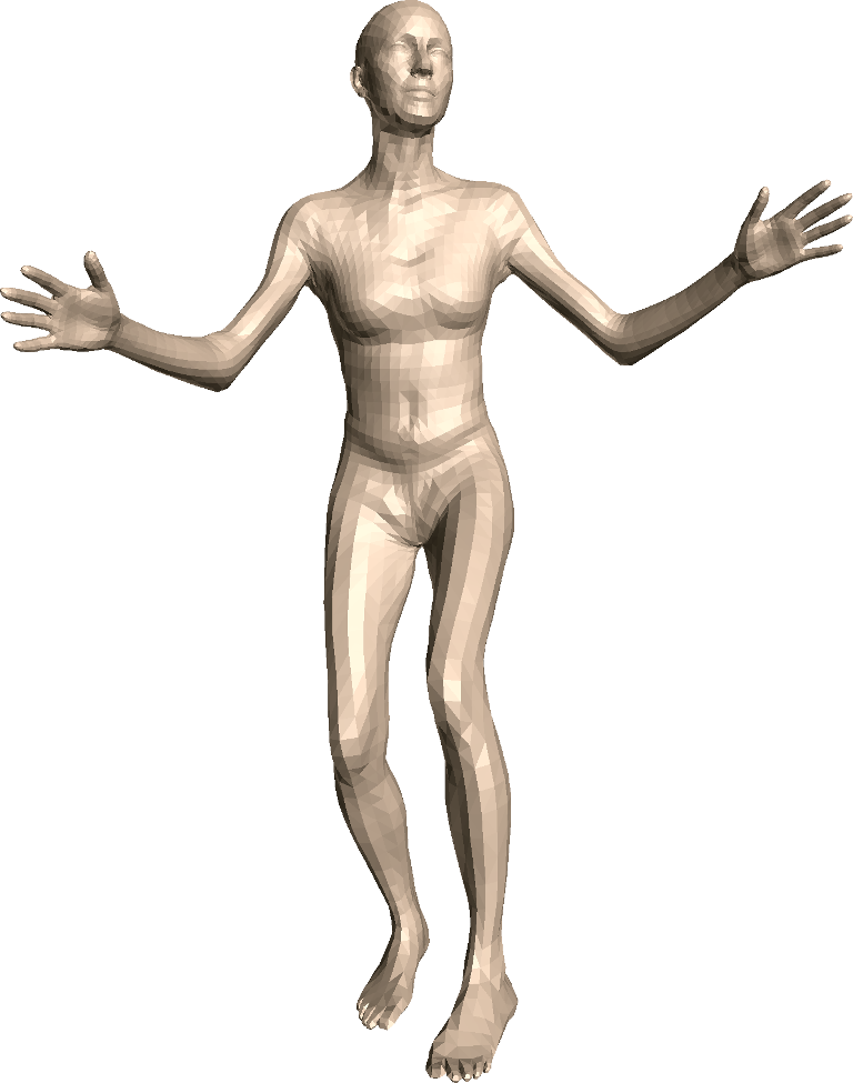
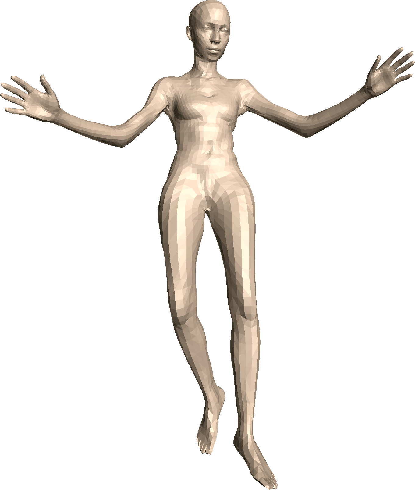
(a) FAKIR	(b) SMPLify + DeepCut 2D	(c) SMPLify + DeepCut 3D	(d) SMPLify + FAKIR	(e) FARM

Figure 18: Comparison with SMPLify on the Danseuse with Crotales. (a) FAKIR registration; (b) SMPLify using DeepCut predicted 3D joint positions on a single rendering; (c) SMPLify using DeepCut predicted 3D joint positions on two rendered views; (d) SMPLify using 3D joint positions estimated by FAKIR; (e) FARM registration. (First row: overlayed registered model; Second row: registered model)

Computation Time

The computational bottleneck of FAKIR lies in the assignment of each point several times during the optimization process. This assignment is updated after each bone parameter change. However, the number of updates is related to the geometry of the surface and not to the number of sample points. Therefore, the overall complexity is linear with respect to the number of points. From an experimental point of view, FAKIR is a reasonably light algorithm: for a point cloud of $10000$ points and the 22-bone human model, the first forward pass of FAKIR takes $2.5s$ and the computation time for one pass decreases to $1s$ in average afterwards.

Limitations

Despite its good results, FAKIR has some limitations. First, if two consecutive bones are aligned, their length estimation is not reliable, since the position of the middle joint is undetermined if no proportion constraint is set on the model. This limitation appears on the Aphrodite left leg (Figure 11). We could also improve registration results by adding constraints of symmetry to the energy functions. However these constraints should be quite loose, because of the unrealistic proportions of artistic statues. Furthermore, failure cases include some misalignments due to a local minimum (one of the arms of the mermaid in Figure 13, the feet of the shape on the top-right of Figure 14 and the back leg of the centaur in Figure 15.) Further local extrinsic refinement would improve the result. In addition, a process of local modification of the skeleton structure could be carried on, followed by an update of its registration. Last, to avoid any manual intervention, we have tested an automatic approach by initializing the pelvis in the center of the bounding box of the points and by orienting it upwards. This initialization is effective for most standing statues (results provided in the supplementary material). Using principal component analysis to initialize the orientation of the body would also improve the registration for classical human poses (e.g. walking, sitting, lying down). However, the handling of the relaxation process at bifurcations could also be improved. Currently, the position of the pelvis is not updated by exploiting the whole information arising from the registration of all the incident branches.

5 Conclusion and perspectives

We introduced a sphere-mesh anatomical model and a combined calibration and registration algorithm to estimate the anatomy and the pose of digitized archaeological statues. Our algorithm is useful when it is not possible to extract a shape template from a statistical analysis of examples representative of the diversity of poses and morphologies. Given the simplicity of our anatomical model, it is very easy to adapt it to many shapes, such as animals or imaginary creatures. While our method already gives good results, a further improvement would be to handle the case of a clothed statue.

Acknowledgments

This work was funded by the e-Roma project from the French Agence Nationale de la Recherche (ANR-16-CE38-0009). The Dancer with crotales model is a point set of the Farman Dataset [DAL^∗11]. The other 8 statues data are sampled on meshes from the Sketchfab website: the Venus de Milo model is courtesy of Sketchfab user "tux", the Dancing Faun model is courtesy of Moshe Caine and the other 5 statues models (Aphrodite, Old Man Walking, Esquiline Venus, Old Fisherman and Mermaid) are courtesy of Geoffrey Marchal. We thank Riccardo Marin for sharing his FARM registration results.

References

- [AL11] Aristidou A., Lasenby J.: FABRIK: A fast, iterative solver for the inverse kinematics problem. Graph. Models 73, 5 (2011), 243–260.
- [AMB∗19] Alldieck T., Magnor M., Bhatnagar B. L., Theobalt C., Pons-Moll G.: Learning to reconstruct people in clothing from a single rgb camera, 2019. arXiv:1903.05885.
- [AMX∗18] Alldieck T., Magnor M., Xu W., Theobalt C., Pons-Moll G.: Video based reconstruction of 3d people models, 2018. arXiv:1803.04758.
- [ARM∗19] Angles B., Rebain D., Macklin M., Wyvill B., Barthe L., Lewis J. P., von der Pahlen J., Izadi S., Valentin J. P. C., Bouaziz S., Tagliasacchi A.: VIPER: volume invariant position-based elastic rods. arXiv:1906.05260.
- [ASK∗05] Anguelov D., Srinivasan P., Koller D., Thrun S., Rodgers J., Davis J.: Scape: shape completion and animation of people. ACM TOG 24 (2005), 408–416.
- [Bas00] Bastioni M.: Make human: Open source tool for making 3d characters. http://www.makehumancommunity.org/, 2000.
- [BBK08] Bronstein A., Bronstein M., Kimmel R.: Numerical Geometry of Non-Rigid Shapes. Springer, 2008.
- [BBLR15] Bogo F., Black M. J., Loper M., Romero J.: Detailed full-body reconstructions of moving people from monocular RGB-D sequences. In ICCV (2015), pp. 2300–2308.
- [BK00] Barron C., Kakadiaris I. A.: Estimating anthropometry and pose from a single image. In CVPR (2000), vol. 1, pp. 669–676 vol.1.
- [BKL∗16] Bogo F., Kanazawa A., Lassner C., Gehler P., Romero J., Black M. J.: Keep it SMPL: Automatic estimation of 3D human pose and shape from a single image. In ECCV (2016), pp. 561–578.
- [Blu67] Blum H.: A Transformation for Extracting New Descriptors of Shape. In Models for the Perception of Speech and Visual Form, Wathen-Dunn W., (Ed.). MIT Press, 1967, pp. 362–380.
- [BP07] Baran I., Popović J.: Automatic rigging and animation of 3d characters. ACM TOG 26, 3 (2007).
- [BS91] Bloomenthal J., Shoemake K.: Convolution surfaces. In Siggraph 91 (1991), ACM, pp. 251–256.
- [CHS∗18] Cao Z., Hidalgo G., Simon T., Wei S.-E., Sheikh Y.: OpenPose: realtime multi-person 2D pose estimation using Part Affinity Fields. In arXiv preprint arXiv:1812.08008 (2018).
- [DAL∗11] Digne J., Audfray N., Lartigue C., Mehdi-Souzani C., Morel J.-M.: Farman Institute 3D Point Sets - High Precision 3D Data Sets. IPOL (2011).
- [GD96] Gavrila D., Davis L. S.: 3-d model-based tracking of humans in action: a multi-view approach. CVPR (1996), 73–80.
- [GSA∗09] Gall J., Stoll C., Aguiar E., Theobalt C., Rosenhahn B., Seidel H.-P.: Motion capture using joint skeleton tracking and surface estimation. CVPR (2009).
- [HBL∗17] Huang Y., Bogo F., Lassner C., Kanazawa A., Gehler P. V., Romero J., Akhter I., Black M. J.: Towards accurate marker-less human shape and pose estimation over time. In 3DV (2017).
- [HDD∗92] Hoppe H., DeRose T., Duchamp T., McDonald J., Stuetzle W.: Surface reconstruction from unorganized points. SIGGRAPH Comput. Graph. 26, 2 (July 1992), 71–78. URL: https://doi.org/10.1145/142920.134011, doi:10.1145/142920.134011.
- [HLRB12] Hirshberg D. A., Loper M., Rachlin E., Black M. J.: Coregistration: Simultaneous alignment and modeling of articulated 3d shape. In ECCV (2012), Fitzgibbon A., Lazebnik S., Perona P., Sato Y., Schmid C., (Eds.), pp. 242–255.
- [HSR∗09] Hasler N., Stoll C., Rosenhahn B., Thormählen T., Seidel H.-P.: Estimating body shape of dressed humans. Computers & Graphics (SMI 2009) 33, 3 (2009), 211 – 216.
- [HSS∗09] Hasler N., Stoll C., Sunkel M., Rosenhahn B., Seidel H.-P.: A statistical model of human pose and body shape. CGF, Proc. Eurographics 28 (2009).
- [Hus55] Hus A.: Sculpture étrusque archaïque : le cavalier marin de la villa giulia. Mélanges de l’école française de Rome 67, 1 (1955), 69–126.
- [HWCO∗13] Huang H., Wu S., Cohen-Or D., Gong M., Zhang H., Li G., B.Chen: L1-medial skeleton of point cloud. ACM TOG 32, 4 (2013), 65:1–65:8.
- [JCZ19] Jiang H., Cai J., Zheng J.: Skeleton-aware 3d human shape reconstruction from point clouds. In ICCV 2019 (2019).
- [JLW10] Ji Z., Liu L., Wang Y.: B-mesh: A modeling system for base meshes of 3d articulated shapes. Comput. Graph. Forum 29 (2010), 2169–2177.
- [LGK∗12] Lee D., Glueck M., Khan A., Fiume E., Jackson K.: Modeling and simulation of skeletal muscle for computer graphics: A survey. Foundations and Trends® in Computer Graphics and Vision 7 (2012), 229.
- [LIPM19] Lazova V., Insafutdinov E., Pons-Moll G.: 360-degree textures of people in clothing from a single image, 2019. arXiv:1908.07117.
- [LMR∗15] Loper M., Mahmood N., Romero J., Pons-Moll G., Black M. J.: SMPL: A skinned multi-person linear model. ACM TOG (Proc. SIGGRAPH Asia) 34, 6 (2015), 248:1–248:16.
- [LRB∗16] Litany O., Rodolà E., Bronstein A., Bronstein M., Cremers D.: Non-rigid puzzles. Computer Graphics Forum 35 (2016), 135–143.
- [LSS∗19] Li C., Simon T., Saragih J. M., Póczos B., Sheikh Y.: LBS autoencoder: Self-supervised fitting of articulated meshes to point clouds. In CVPR 2019 (2019).
- [MMRC20] Marin R., Melzi S., Rodolà E., Castellani U.: Farm: Functional automatic registration method for 3d human bodies. Computer Graphics Forum 39, 1 (2020), 160–173.
- [New34] Newell A. N.: Gallo-roman religious sculpture. Greece and Rome 3, 8 (1934), 74–84.
- [PF01] Plankers R., Fua P.: Articulated soft objects for video-based body modeling. In ICCV (2001), vol. 1, pp. 394–401 vol.1.
- [PIT∗16] Pishchulin L., Insafutdinov E., Tang S., Andres B., Andriluka M., Gehler P., Schiele B.: Deepcut: Joint subset partition and labeling for multi person pose estimation. In IEEE Conference on Computer Vision and Pattern Recognition (CVPR) (2016).
- [PMPHB17] Pons-Moll G., Pujades S., Hu S., Black M.: Clothcap: Seamless 4d clothing capture and retargeting. ACM TOG, (Proc. SIGGRAPH) 36, 4 (2017).
- [PMRMB15] Pons-Moll G., Romero J., Mahmood N., Black M. J.: Dyna: A model of dynamic human shape in motion. ACM TOG, (Proc. SIGGRAPH) 34, 4 (2015), 120:1–120:14.
- [RTTP17] Remelli E., Tkach A., Tagliasacchi A., Pauly M.: Low-dimensionality calibration through local anisotropic scaling for robust hand model personalization. In ICCV (2017).
- [SBB10] Sigal L., Balan A., Black M. J.: HumanEva: Synchronized video and motion capture dataset and baseline algorithm for evaluation of articulated human motion. IJCV 87, 1 (2010), 4–27.
- [SBR∗04] Sigal L., Bhatia S., Roth S., Black M. J., Isard M.: Tracking loose-limbed people. In CVPR (2004), vol. 1, pp. I–I.
- [SCYW16] Sun F., Choi Y.-K., Yu Y., Wang W.: Medial meshes – a compact and accurate representation of medial axis transform. IEEE TVCG 22 (2016), 1278–1290.
- [SHG∗11] Stoll C., Hasler N., Gall J., Seidel H.-P., Theobalt C.: Fast articulated motion tracking using a sums of gaussians body model. pp. 951–958.
- [TDS∗16] Tagliasacchi A., Delame T., Spagnuolo M., Amenta N., Telea A.: 3d skeletons: A state-of-the-art report. Computer Graphics Forum 35 (2016).
- [TGB13] Thiery J.-M., Guy E., Boubekeur T.: Sphere-meshes: Shape approximation using spherical quadric error metrics. ACM TOG (Proc. SIGGRAPH Asia 2013) 32, 6 (2013).
- [TPT16] Tkach A., Pauly M., Tagliasacchi A.: Sphere-meshes for real-time hand modeling and tracking. ACM TOG 35, 6 (2016), 222:1–222:11.
- [TTR∗17] Tkach A., Tagliasacchi A., Remelli E., Pauly M., Fitzgibbon A.: Online generative model personalization for hand tracking. ACM TOG 36 (2017), 1–11.
- [TZMS04] Theobalt C., Ziegler G., Magnor M., Seidel H.-P.: Model-based free-viewpoint video: Acquisition, rendering, and encoding. Picture Coding Symposium (2004).
- [WC91] Wang L.-C. T., Chen C.-C.: A combined optimization method for solving the inverse kinematics problems of mechanical manipulators. IEEE Trans. Robotics and Automation 7 (1991), 489–499.
- [WHB11] Weiss A., Hirshberg D., Black M. J.: Home 3d body scans from noisy image and range data. In ICCV (2011), pp. 1951–1958.
- [WZC12] Wei X., Zhang P., Chai J.: Accurate realtime full-body motion capture using a single depth camera. ACM TOG 31 (2012).
- [YZZ∗19] Yu T., Zheng Z., Zhong Y., Zhao J., Dai Q., Pons-Moll G., Liu Y.: Simulcap : Single-view human performance capture with cloth simulation, 2019. arXiv:1903.06323.
- [ZB15] Zuffi S., Black M. J.: The stitched puppet: A graphical model of 3D human shape and pose. In CVPR (2015), pp. 3537–3546.
- [ZPBPM17] Zhang C., Pujades S., Black M. J., Pons-Moll G.: Detailed, accurate, human shape estimation from clothed 3d scan sequences. In CVPR (2017).