Correlation functions in ${\cal N}=2$ Supersymmetric vector matter Chern-Simons theory

Abstract

We compute the two, three point function of the opearators in the spin zero multiplet of ${\cal N}=2$ Supersymmetric vector matter Chern-Simons theory at large $N$ and at all orders of ’t Hooft coupling by solving the Schwinger-Dyson equation. Schwinger-Dyson method to compute four point function becomes extremely complicated and hence we use bootstrap method to solve for four point function of scaler operator $J_{0}^{f}=\bar{\psi}\psi$ and $J_{0}^{b}=\bar{\phi}\phi$. Interestingly, due to the fact that $\langle J_{0}^{f}J_{0}^{f}J_{0}^{b}\rangle$ is a contact term, the four point function of $J_{0}^{f}$ operator looks like that of free theory up to overall coupling constant dependent factors and up to some bulk AdS contact terms. On the other hand the $J_{0}^{b}$ four-point function receives an additional contribution compared to the free theory expression due to the $J_{0}^{f}$ exchange. Interestingly, double discontinuity of this single trace operator $J_{0}^{f}$ vanishes and hence it only contributes to AdS-contact term.

1 Introduction

The perturbative technique to compute observables in quantum field theories involving Feynman diagrams is effective only when the coupling is weak and breaks down in the strong coupling regime. In the past few decades, various strong-weak dualities have been discovered proving to be extremely useful in understanding some of the most interesting non-perturbative properties of strongly coupled quantum field theories. One such class of dualities which have been studied extensively in recent times are the Bosonization dualities in Chern Simons gauge theories coupled to fundamental matter at large $N$ [1, 2, 3, 4, 5, 6]. Though, one of the main indications for these dualities initially came from their holographic duality with Vasiliev theories in $AdS_{4}$ [7, 8, 9, 10, 11, 12], by now there exists a plethora of evidence for these dualities coming from exact computations of correlation functions, thermal partition functions, scattering amplitudes and RG flow analysis relating these theories to known supersymmetric dualities [13, 14, 15, 16, 17, 18, 19, 20, 21, 22, 23, 24, 25, 26, 27, 28, 29, 3, 4, 5, 30, 31, 32, 33].

Primary example of these bosonization dualities are those among the quasi-fermionic (critical bosonic and regular fermionic theory) and the quasi-bosonic theories (regular bosonic and critical fermionic theory). A particularly interesting case of these dualities is present in the ${\cal N}=2$ supersymmetric $U(N)$ Chern Simons theory coupled to a single fundamental chiral multiplet. This theory exhibits a strong-weak self duality [34, 35, 36] generalizing the well known Giveon-Kutosov duality [37, 34]. The self duality of this supersymmetric theory serves as a parent duality for the non-supersymmetric bosonization dualities mentioned above since they can obtained from the supersymmetric theory via RG flows seeded by mass deformations [38, 39]. Taking hints from the supersymmetric dualities and the Level-Rank duality of pure Chern Simons theory, finite $N$ extensions for the non supersymmetric dualities have also been proposed [40, 41, 42, 43, 44, 45, 46, 47, 48, 49]. These theories were also investigated recently in presence of background magnetic field [50].

In this article, we will focus our attention on the ${\cal N}=2$ theory. Various large $N$ computations in this theory show remarkable features which are absent in the non supersymmetric couterparts. For example, the all loop $2\to 2$ scattering amplitude is tree-level exact except in anyonic channel [26] and it was shown that these amplitudes are also invariant under Dual superconformal symmetry [26, 29]. [28] further showed that the tree level $m\to n$ scattering amplitudes in this theory can be constructed using the BCFW recursions relations.

Although many interesting non supersymmetric physical observables, as mentioned above, are amenable to direct exact computations by solving corresponding Dyson-Schwinger equations, the computation of 4-point correlation function of even the simplest of single trace operators, namely the scalar operators $\bar{\phi}\phi$ and $\bar{\psi}\psi$, appears prohibitively difficult to compute via this direct approach. Given the remarkable simplicity of the results for other known observables one expects the 4-point functions in this theory to also have a simple structure. In the present article, our main goal will be to determine the exact 2, 3 and leading connected 4-point correlation functions of scalar operators in this supersymmetric theory.

For the quasi-bosonic and quasi-fermionic theories mentioned above, [51, 52] recently determined the 4-point function of scalar operator using recently developed ideas from conformal Bootstrap. In particular, one of the central of the central objects used in [51] is the double discontinuity of the 4-point function which determines the coefficients in the OPE expansion of external operators via the Lorenzian inversion formula (LIF) discovered by Caron-Huot in [53]. The authors of [51] first demonstrated that for large-$N$ CFTs the double discontinuity of the 4-point function of identical scalars determines the full 4-point function up to three $AdS_{4}$ contact Witten diagrams. The authors further showed that for the quasi-bosonic and quasi-fermionic theories the coefficients of these contact terms vanish. In the present work, we apply some of these ideas in conjunction with the self duality, to the case of scalar 4-point functions in our $N=2$ theory.

Our article is structured as follows. In section 2, we describe the ${\cal N}=2$ theory of interest in this paper its operators spectrum in some detail. In section 3, we determine the scalar multiplet 2 and 3-point functions via a directly computation. In section 4, we determine the 4-point function of the bosonic and the fermionic scalar operators in this theory using the double discontinuity technique developed in [51]. Finally, in the section 5, we summarize our results and outline related open questions and future directions. In various appendix, we collect our notation and conventions, some technical details of the results in main text of the paper and briefly summarize our attempt at the direct computation of 4-point function.

Note added in the proof :

While we were in the process of finishing up our article, we were informed about the related work [54] by the authors which has overlap with the results of our section 3.

2 ${\cal N}=2$ theory and its Operator Spectrum

In this paper, we are interested in ${\cal N}=2$ $U(N)$ Chern-Simons theory coupled to single chiral multiplet, $\Phi\equiv(\phi,\psi)$, in the fundamental representation of the gauge group. The position space Lagrangian for the theory is

$$\mathcal{S}_{\mathcal{N}=2}^{L}=\int d^{3}x\biggl{[} -\frac{\kappa}{4\pi}\epsilon^{\mu\nu\rho}\text{Tr}\left(A_{\mu}\partial_{\nu}A_{\rho}-\frac{2i}{3}A_{\mu}A_{\nu}A_{\rho}\right)-\bar{\psi}i\not{\mathcal{D}}\psi+\mathcal{D}^{\mu}\bar{\phi}\mathcal{D}_{\mu}\phi$$

$$+\frac{4\pi^{2}}{\kappa^{2}}(\bar{\phi}\phi)^{3}-\frac{4\pi}{\kappa}(\bar{\phi}\phi)(\bar{\psi}\psi)-\frac{2\pi}{\kappa}(\bar{\psi}\phi)(\bar{\phi}\psi)\biggr{]}\ .$$ (2.1)

The theory above has two parameters : the rank of the gauge group, $N$, and the Chern-Simons level, $\kappa$, which is quantized to take only integer values [55]. $\kappa^{-1}$ controls the strength of gauge interactions and the theory is perturbative for large values of $\kappa$ at any finite $N$.

This theory is conjectured to be self-dual under a strong-weak type duality, [34]. In the ’t Hooft like large $N$ limit

$$\kappa\rightarrow\infty,N\rightarrow\infty\quad\textrm{with}\quad\lambda=\frac{N}{\kappa}\quad\textrm{fixed}$$ (2.2)

of interest in this paper, the duality transformation is

$$\kappa=-\kappa,\quad\lambda=\lambda-\text{sgn}(\lambda)\ .$$ (2.3)

Apart from the matching of many of the supersymmetric observables which can be computed at finite $N$ and $\kappa$ using supersymmetric localization techniques, recent exact computation of many non-supersymmetric observables, e.g. the thermal partition function, in the large $N$ limit [2, 1, 5, 30, 38, 25] has provided ample evidence for this conjectured duality.

The theory is quantum mechanically (super) conformal for all values of $\kappa$ and $N$. In the ’t Hooft limit, one can focus on the single trace superconformal primary operator spectrum of the theory. Though our theory has ${\cal N}=2$ superconformal symmetry, in this paper we will work in the ${\cal N}=1$ superspace formulation to allow us to use the relevant results of [26] for our computations. In the ${\cal N}=1$ language, the operators spectrum of the theory consists of a set of supercurrent operators [56]

$$J^{(s)}=\sum_{r=0}^{2s}(-1)^{\frac{r(r+1)}{2}}\begin{pmatrix}2s\\ r\end{pmatrix}\nabla^{r}\bar{\Phi}\nabla^{2s-r}\Phi~{},$$ (2.4)

which are written in terms of the superfields,

$$\Phi=\phi+\theta\psi-\theta^{2}F,\quad\bar{\Phi}=\bar{\phi}+\theta\bar{\psi}-\theta^{2}\bar{F}~{}.$$

and the superscript $s$ in(2.4) takes values in $\{0,\frac{1}{2},1,\frac{3}{2},\ldots\}$. Here, we have also defined

$$\begin{split}J^{(s)}=&\lambda^{\alpha_{1}}\lambda^{\alpha_{2}}\ldots\lambda^{\alpha_{2s}}\mathcal{J}_{\alpha_{1}\alpha_{2}\ldots\alpha_{2s}},\quad\nabla=\lambda^{\alpha}\nabla_{\alpha}\end{split}$$ (2.5)

using the auxiliary commuting polarisation spinors, $\lambda^{\alpha_{i}}$, which keep track of the spin; and $\nabla_{\alpha_{i}}$ are the standard supersymmetry invariant gauge-covariant derivatives. Their action on the matter superfields of our theory is given by,

$$\nabla_{\alpha}\Phi= D_{\alpha}\Phi-i\Gamma_{\alpha}\Phi$$

$$\nabla_{\alpha}\bar{\Phi}= D_{\alpha}\bar{\Phi}+i\Gamma_{\alpha}\bar{\Phi}$$ (2.6)

The explicit expressions for the first few spin-$s$ currents are,

$$J_{0} =\bar{\Phi}\Phi$$ (2.7)

$$J_{\alpha} =\bar{\Phi}\nabla_{\alpha}\Phi-\nabla_{\alpha}\bar{\Phi}\Phi=\bar{\Phi}D_{\alpha}\Phi-D_{\alpha}\bar{\Phi}\Phi-2i\bar{\Phi}\Gamma_{\alpha}\Phi$$

$$J_{\alpha\beta} =\bar{\Phi}\nabla_{\alpha}\nabla_{\beta}\Phi-2\nabla_{\alpha}\bar{\Phi}\nabla_{\beta}\Phi+\nabla_{\alpha}\nabla_{\beta}\bar{\Phi}\Phi$$

$$J_{\alpha\beta\gamma} =\bar{\Phi}\nabla_{\alpha}\nabla_{\beta}\nabla_{\gamma}\Phi-3\nabla_{\alpha}\bar{\Phi}\nabla_{\beta}\nabla_{\gamma}\Phi-3\nabla_{\alpha}\nabla_{\beta}\bar{\Phi}\nabla_{\gamma}\Phi+\nabla_{\alpha}\nabla_{\beta}\nabla_{\gamma}\bar{\Phi}\Phi$$

In the free limit of the theory i.e. $\lambda\rightarrow 0$, each of these supercurrents, ${\cal J}^{(s)}$ with $s\neq 0$, satisfies the conservation equation

$${\cal D}^{\alpha}\left(\frac{\partial}{\partial\lambda^{\alpha}}{\cal J}^{(s)}\right)=0$$ (2.8)

and constitutes two component conserved current operators $\{J^{(s)},J^{(s+\frac{1}{2})}\}$ in its $\theta$ expansion [56]. At finite $\lambda$, the conservation equation (2.8) is violated at order $\frac{1}{N}$ by double trace operators [56, 1].

In this article, we are interested in the scalar operator ${\cal J}^{(0)}(\theta,x)$. There is no conservation equation associated with this operator and it constitutes 2 scalar and 1 spin half operator as follows

$$J^{(0)}(\theta,x)=J_{0}^{b}(x)+\theta^{\alpha}\Psi_{\alpha}(x)-\theta^{2}J_{0}^{f}(x)\$$ (2.9)

where

$$J_{0}^{b}(x)=\bar{\phi}\phi(x),\quad\Psi_{\alpha}(x)=(\bar{\phi}\psi_{\alpha}+\bar{\psi}_{\alpha}\phi)(x),\quad J_{0}^{f}(x)=\bar{\psi}\psi(x).$$ (2.10)

In the subsequent sections, we compute the 2 and 3-point functions of the $J^{(0)}$ operator and two component of the 4-point function.

3 Correlation functions

In this section, we compute the two and three point correlation function of the $J_{0}(\theta,p)$ operator. Two of the main ingredients for these computations are the exact propagator (3.2) and the renormalized four point vertex for the fundamental superfield $\Phi(\theta,p)$ ($\nu_{4}$ in 3.3). These were computed in [26] for a more general class of theories with ${\cal N}=1$ supersymmetry which can be thought of as one parameter deformation of the ${\cal N}=2$ theory of interest in this paper. Below, we list these results for our ${\cal N}=2$ theory, conveniently stated in term of the exact quantum effective action

$$\begin{split}S&=S_{2}+S_{4}~{},\\ S_{2}&=\int\frac{d^{3}p}{(2\pi)^{3}}d^{2}\theta_{1}d^{2}\theta_{2}\left[\bar{\Phi}(\theta_{1},-p)e^{-\theta_{1}^{\alpha}p_{\alpha\beta}\theta_{2}^{\beta}}\Phi(\theta_{2},p)\right],\\ S_{4}&=\frac{1}{2}\int\frac{d^{2}p}{(2\pi)^{3}}\frac{d^{2}q}{(2\pi)^{3}}\frac{d^{2}k}{(2\pi)^{3}}d^{2}\theta_{1}d^{2}\theta_{2}d^{2}\theta_{3}d^{2}\theta_{4}\\ &\hskip 42.67912pt\bigg{[}\nu_{4}(\theta_{1},\theta_{2},\theta_{3},\theta_{4};p,q,k)\Phi_{i}(\theta_{1},-(p+q))\bar{\Phi}^{i}(\theta_{2},p)\bar{\Phi}^{j}(\theta_{3},k+q)\Phi_{j}(\theta_{4},-k)\bigg{]}\\ \end{split}$$ (3.1)

The quadratic part of the effective action receives no quantum corrections at large $N$ in the ${\cal N}=2$ theory. The propagator is thus tree level exact and given by

$$\begin{split}\langle\bar{\Phi}(\theta_{1},p_{1})\Phi(\theta_{2},p_{2})\rangle&=(2\pi)^{3}\delta^{3}(p_{1}+p_{2}){\cal P}(\theta_{1},\theta_{2};p_{1})\\ &=(2\pi)^{3}\delta^{3}(p_{1}+p_{2})\frac{e^{-\theta^{\alpha}_{1}\theta^{\beta}_{2}(p_{1})_{\alpha\beta}}}{p_{1}^{2}}.\end{split}$$ (3.2)

The quartic superspace vertex, $\nu_{4}$, does receive quantum corrections and takes the following form

$$\nu_{4}(\theta_{1},\theta_{2},\theta_{3},\theta_{4};p,q,k) =e^{\frac{1}{4}X.(p.X_{12}+q.X_{13}+k.X_{43})}F_{4}(X_{12},X_{13},X_{43};p,q,k),$$ (3.3)

$$\textrm{with}\quad F_{4} =X_{12}^{+}X_{43}^{+}\bigg{[}A(p,q,k)X_{12}^{-}X_{43}^{-}X_{13}^{+}X_{13}^{-}+C(p,q,k)X_{12}^{-}X_{13}^{+}$$

$$\hskip 142.26378pt+D(p,q,k)X_{13}^{+}X_{43}^{-}\bigg{]}$$

The overall exponential factor is determined by supersymmetric Ward identity (3.7), while the coefficient functions A, C and D require explicit computation and given by [26]

$$\begin{split}A(p,q,k)&=-\frac{2\pi i}{\kappa}e^{2i\lambda\left[\tan^{-1}\left(\frac{2k_{s}}{q_{3}}\right)-\tan^{-1}\left(\frac{2p_{s}}{q_{3}}\right)\right]},\\ C(p,q,k)&=D(p,q,k)=\frac{2A(p,q,k)}{(k-p)_{-}}.\\ \end{split}$$ (3.4)

Note that the vertex $\nu_{4}$ was computed in a special momentum configuration, namely

$$q_{+}=q_{-}=0.$$ (3.5)

while the momenta $p$ and $k$ are arbitrary . For this reason, our computation of correlation functions will also be restricted configuration in which the momentum of $J_{0}$ operators are restricted to lie only in the 3-direction. Diagrammatically, the exact four point vertex will be represented as in Figure 1.

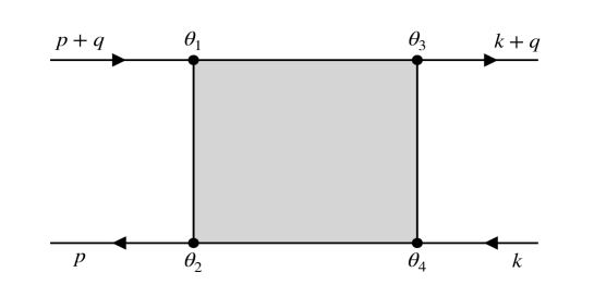
Figure 1: Diagrammatic representation of the exact four point vertex, $\nu_{4}$ in (3.3).

3.1 Constraints on correlation functions from supersymmetry

To begin with, let us study the constraints on an arbitrary correlation function due to supersymmetry. As stated earlier, although our theory has ${\cal N}=2$ supersymmetry, we will be working in ${\cal N}=1$ superspace following [26]. A general n-point correlation function of ${\cal N}=1$ scalar superfield is constrained by supersymmetry and translation invariance to take the following form [26]

$$\begin{split}&\langle{\cal O}_{1}(\theta_{1},p_{1})\ldots{\cal O}_{n}(\theta_{n},p_{n})\rangle\\ &\qquad=(2\pi)^{3}\delta^{3}\left(\sum_{i=1}^{n}p_{i}\right)\exp\left[\left(\frac{1}{n}\sum_{i=1}^{n}\theta_{i}\right).\left(\sum_{i=1}^{n}p_{i}.\theta_{i}\right)\right]F_{n}(\{\theta_{in}\};\{p_{i}\})\end{split}$$ (3.6)

where $\theta_{ij}=\theta_{i}-\theta_{j}$. The $\delta^{3}(\sum_{i}p_{i})$ follows from translation invariance while the overall Grassmann exponential factor follows from invariance under ${\cal N}=1$ supersymmetry. Note that the function $F_{n}$ above only depend on the differences of the Grassmann coordinates. Following [26], the form is easily derived as follows

$$\begin{split}0&=\left[\sum_{i=1}^{n}{\cal Q}^{(i)}_{\alpha}\right]\langle{\cal O}_{1}(\theta_{1},p_{1})\ldots{\cal O}_{n}(\theta_{n},p_{n})\rangle\\ &=\left[\sum_{i=1}^{n}\left(\frac{\partial}{\partial\theta_{i}^{\alpha}}-(p_{i})_{\alpha\beta}\theta_{i}^{\beta}\right)\right]\langle{\cal O}_{1}(\theta_{1},p_{1})\ldots{\cal O}_{n}(\theta_{n},p_{n})\rangle\\ &=\left(n\frac{\partial}{\partial X^{\alpha}}-\sum_{i=1}^{n-1}(p_{i})_{\alpha\beta}X_{in}^{\beta}\right)\langle{\cal O}_{1}(\theta_{1},p_{1})\ldots{\cal O}_{n}(\theta_{n},p_{n})\rangle\\ \end{split}$$ (3.7)

In the last line above, we used the momentum conservation to replace $p_{n}$ with $\sum_{i=1}^{n-1}(-p_{i})$. Defining the sum and the difference of Grassmann variables as

$$X^{\alpha}=\sum_{i=1}^{n}\theta_{i}^{\alpha}\quad,\quad X_{in}^{\alpha}=\theta_{i}^{\alpha}-\theta_{n}^{\alpha}.$$ (3.8)

The factorised form in (LABEL:widen) follows as the solution to last equation in (3.7).

3.2 $J_{0}$-vertex

Before proceeding to the computation of correlation functions, it would be useful to compute an intermediate quantity, the $J_{0}$-vertex. It is defined by stripping of the propagators from $\langle J_{0}\Phi\bar{\Phi}\rangle$ as follows

$$\begin{split}&\langle J_{0}(\theta_{1},p_{1})\Phi(\theta_{2},p_{2})\bar{\Phi}(\theta_{3},p_{3})\rangle=\\ &\quad\int\frac{d^{3}p^{\prime}_{2}}{(2\pi)^{3}}\frac{d^{3}p^{\prime}_{3}}{(2\pi)^{3}}d^{2}\theta^{\prime}_{2}d^{2}\theta^{\prime}_{3}~{}\left[\langle J_{0}(\theta_{1},p_{1})\Phi(\theta^{\prime}_{2},p^{\prime}_{2})\bar{\Phi}(\theta^{\prime}_{3},p^{\prime}_{3})\rangle_{ver}{\cal P}(\theta^{\prime}_{2},\theta_{2};-p_{2}){\cal P}(\theta^{\prime}_{3},\theta_{3};p_{3})\right]\\ \end{split}$$ (3.9)

and satisfies the same Ward identity as a three point function (LABEL:widen).

The vertex receives contribution both from the free propagation of the fundamental field as well as from the interaction vertices in the theory. The free part vertex is simply proportional to the momentum and the Grassmannian $\delta$-functions while the interacting part of the vertex can be computed from the exact $\nu_{4}$ vertex. Figure (2) shows the relevant diagrams.

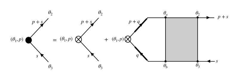
Figure 2: Solid circle on the LHS represents the full exact $J_{0}$ vertex and the first diagram on RHS is the free vertex. The second diagram on RHS includes all the interactions which are accounted by insertion of exact 4 point vertex (3.3) connected to the external ${\cal J}^{(0)}$ operator using the exact propagator.

$$\begin{split}&\langle J_{0}(\theta_{1},p)\Phi(\theta_{2},r)\bar{\Phi}(\theta_{3},s)\rangle_{ver}=\langle J_{0}(\theta_{1},p)\Phi(\theta_{2},r)\bar{\Phi}(\theta_{3},s)\rangle_{ver,free}+\langle J_{0}(\theta_{1},p)\Phi(\theta_{2},r)\bar{\Phi}(\theta_{3},s)\rangle_{ver,int}\\ &\\ &\textrm{where}\quad\langle J_{0}(\theta_{1},p)\Phi(\theta_{2},r)\bar{\Phi}(\theta_{3},s)\rangle_{ver,free}=(2\pi)^{3}\delta^{3}(p+r+s)\ \ \nu_{3,free}(\theta_{12},\theta_{32};p,s)\\ &\hskip 179.25244pt=(2\pi)^{3}\delta^{3}(p+r+s)\theta_{32}^{+}\theta_{32}^{-}\theta_{12}^{+}\theta_{12}^{-}\\ &\textrm{and}\quad\langle J_{0}(\theta_{1},p)\Phi(\theta_{2},r)\bar{\Phi}(\theta_{3},s)\rangle_{ver,int}\\ &\qquad=(2\pi)^{3}\delta^{3}(p+r+s)\left[\int\frac{d^{3}q}{(2\pi^{3})}d^{2}\theta_{a}d^{2}\theta_{b}~{}{\cal P}(\theta_{1},\theta_{a};q+p){\cal P}(\theta_{b},\theta_{1};q)\nu_{4}(\theta_{a},\theta_{b},\theta_{2},\theta_{3};q,p,s)\right]\\ &\qquad=(2\pi)^{3}\delta^{3}(p+r+s)e^{\frac{1}{3}\theta_{123}.(p.\theta_{12}+s.\theta_{32})}\nu_{3,int}(\theta_{12},\theta_{32},p,s)\\ \end{split}$$ (3.10)

Explicit computation of the above integral, with constraint $p_{+}=p_{-}=0$ following from the (3.5), leads to the following result for the full $J_{0}$-vertex factor

$$\begin{split}\nu_{3}&=\left(\nu_{3,free}+\nu_{3,int}\right)(\theta_{12},\theta_{32},p,s)\\ &=\frac{1}{2s^{+}}\left[1-e^{2i\lambda\tan^{-1}(\frac{2s_{s}}{p_{3}})}\right]\theta_{32}^{+}\theta_{12}^{+}+\frac{1}{2p_{3}}\left(e^{2i\lambda\tan^{-1}(\frac{2s_{s}}{p_{3}})-i\pi\lambda sgn(p_{3})}-1\right)\theta_{32}^{+}\theta_{32}^{-}\\ &\qquad+\left(1+\frac{1}{6}(-4+e^{2i\lambda\tan^{-1}(\frac{2s_{s}}{p_{3}})}+3e^{2i\lambda\tan^{-1}(\frac{2s_{s}}{p_{3}})-i\pi\lambda sgn(p_{3})})\right)\theta_{32}^{+}\theta_{32}^{-}\theta_{12}^{+}\theta_{12}^{-}\end{split}$$ (3.11)

The $J_{0}$-vertex computed above will be useful in further computations of 2 and 3 point functions of the $J_{0}$ operator.

3.3 $\langle J_{0}J_{0}\rangle$ correlation function

The 2 point function can be straightforwardly computed from the $J_{0}$-vertex determined in the previous section by combining the exact vertex on one side with the free vertex on the other side. Figure (3) shows the relevant diagram which leads to the following integral for the two point function

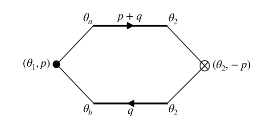
Figure 3: The full $J_{0}$ 2 point function is obtained by connecting the exact $J_{0}$-vertex (solid circle) to the free vertex (cross) with exact propagators (thick line).

$$\begin{split}&\langle J_{0}(\theta_{1},p)J_{0}(\theta_{2},r)\rangle\\ &\quad=(2\pi)^{3}\delta^{3}(p+r)\left[N\int\frac{d^{3}q}{(2\pi)^{3}}d^{2}\theta_{a}d^{2}\theta_{b}~{}\nu_{3}(\theta_{1},\theta_{a},\theta_{b};p,-p-q,q){\cal P}(\theta_{a},\theta_{2};q+p){\cal P}(\theta_{2},\theta_{b};q)\right]\\ \end{split}$$ (3.12)

Again, the collinear constraint (3.5) restricts the momenta $p$ and $s$ to lie in 3-direction. Computing the integrals with this constraint leads to the following result

$$\begin{split}&\langle J_{0}(\theta_{1},p)J_{0}(\theta_{2},r)\rangle\\ &\qquad=(2\pi)^{3}\delta^{3}(p+r)N\frac{e^{-\theta_{1}.p.\theta_{2}}}{8|p_{3}|}\left(\frac{\sin(\pi\lambda)}{\pi\lambda}+|p_{3}|\delta^{2}(\theta_{12})\frac{1-\cos(\pi\lambda)}{\pi\lambda}\right)\\ \end{split}$$ (3.13)

The result can be straightforwardly generalized for arbitrary external momenta to give

$$\begin{split}&\langle J_{0}(\theta_{1},p)J_{0}(\theta_{2},r)\rangle\\ &\qquad=(2\pi)^{3}\delta^{3}(p+r)N\frac{e^{-\theta_{1}.p.\theta_{2}}}{8|p|}\left(\frac{\sin(\pi\lambda)}{\pi\lambda}+|p|\delta^{2}(\theta_{12})\frac{1-\cos(\pi\lambda)}{\pi\lambda}\right)\\ \end{split}$$ (3.14)

The non vanishing component correlators can easily be read off to give

$$\begin{split}&\langle J^{b}_{0}(p)J^{b}_{0}(-p)\rangle=\frac{N}{8|p|}\frac{\sin(\pi\lambda)}{\pi\lambda}\\ &\langle J^{f}_{0}(p)J^{f}_{0}(-p)\rangle=-\frac{N|p|}{8}\frac{\sin(\pi\lambda)}{\pi\lambda}\\ &\langle\Psi_{\alpha}(p)\Psi_{\beta}(-p)\rangle=\frac{N}{8}\left(\frac{p_{\alpha\beta}}{|p|}\frac{\sin(\pi\lambda)}{\pi\lambda}+C_{\alpha\beta}\frac{1-\cos(\pi\lambda)}{\pi\lambda}\right)\\ &\langle J^{b}_{0}(p)J^{f}_{0}(-p)\rangle=-\frac{N}{8}\frac{(1-\cos(\pi\lambda))}{\pi\lambda}\\ \end{split}$$ (3.15)

Let us compare the above two-point functions with the corresponding two-point functions in the regular fermionic and regular bosonic theories studied in [5] and [30] respectively.

Note that as opposed to the regular bosonic and regular fermionic theories studied in [5] and [30], the $\lambda$ dependence of the two-point function of $J^{b}_{0}$ and $J^{f}_{0}$ operators is the same as that of the higher spin currents in the non-supersymmetric cases. Further, using the double trace factorization argument of [20] relating the two-point function of current operators in the supersymmetric and the above mentioned non-supersymmetric theories, we know that the two-point function of all the current operators in our supersymmetric theory is exactly the same as those of the corresponding regular boson/fermion theory. Thus, we see that in our theory the two-point function of scalar operators is the same as that for the higher spin current operators. The reason for this is supersymmetry. Though we are working in ${\cal N}=1$ superspace language, our theory has underlying ${\cal N}=2$ supersymmetry under which the scalar operators $J^{b}_{0},J^{f}_{0}$ belong to the same supersymmetry multiplet as the spin 1 conserved current and thus the two-point function of the two are thus related by supersymmetry.

3.4 $\langle J_{0}J_{0}J_{0}\rangle$ correlation function

The full 3-point function can be constructed by combining three $J_{0}$ vertices with exact propagators. There are two such diagrams shown in figure (4). Each of these two diagrams can easily be shown to be cyclically symmetric and related to each other by pair-exchange of any two $J_{0}$ insertions. An explicit computation of the diagram shows that each of the diagrams is completely symmetric (cyclic as well as under pair-exchange) by itself and the two diagrams are equal. The full 3 point function is then just twice the contribution of the first diagram which we write down below.

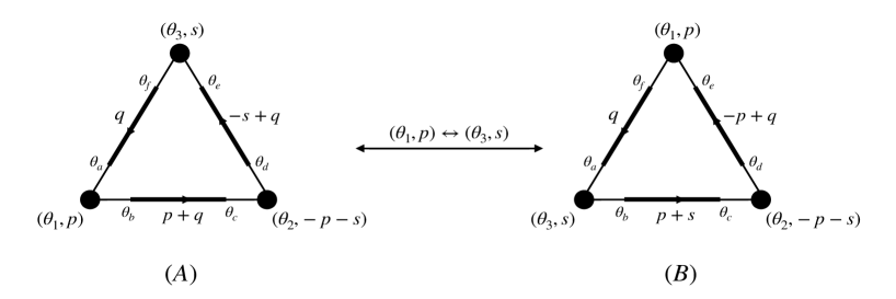
Figure 4: The full $J_{0}$ 3 point function is obtained by connecting three exact $J_{0}$-vertices with exact propagators. There are two such diagrams, as shown above, which turn out to be equal.

$$\begin{split}&\langle J_{0}(\theta_{1},p)J_{0}(\theta_{2},r)J_{0}(\theta_{3},s)\rangle=(2\pi)^{3}\delta^{3}(p+r+s)G_{3}(\theta_{1},\theta_{2},\theta_{3};p,s),\\ &\textrm{where}\\ &\quad G_{3}(\theta_{1},\theta_{2},\theta_{3};p,s)=2N\int\frac{d^{3}q}{(2\pi)^{3}}\left(\prod_{i=a}^{f}d^{2}\theta_{i}\right)\bigg{[}\nu_{3}(\theta_{1},\theta_{a},\theta_{b};p,-p-q)\\ &\hskip 113.81102pt\times\nu_{3}(\theta_{2},\theta_{c},\theta_{d};-p-s,s-q)\ \nu_{3}(\theta_{3},\theta_{e},\theta_{f};s,-q)\\ &\hskip 113.81102pt\times{\cal P}(\theta_{a},\theta_{f};-q){\cal P}(\theta_{a},\theta_{f};s-q){\cal P}(\theta_{c},\theta_{b};-p-q)\bigg{]}\\ \end{split}$$ (3.16)

The overall factor of 2 in the above equation is from the sum over two triangle diagrams in figure (4) which turn out to be equal while the factor of $N$ results from index contractions. Explicit computation of the above integrals in the collinear limit of the external momenta gives the following result

$$\begin{split}&G_{3}(\theta_{1},\theta_{2},\theta_{3};p,s)=e^{\frac{1}{3}\theta_{123}.(p.\theta_{12}+s.\theta_{32})}F_{3}(\theta_{12},\theta_{32},p,s),\\ &\quad F_{3}(\theta_{12},\theta_{32},p,s)=2\left(A_{1}+A_{2}\theta_{12}^{+}\theta_{12}^{-}+A_{3}\theta_{32}^{+}\theta_{32}^{-}+A_{4}\theta_{12}^{+}\theta_{32}^{-}+A_{5}\theta_{32}^{+}\theta_{12}^{-}+A_{6}\theta_{12}^{+}\theta_{12}^{-}\theta_{32}^{+}\theta_{32}^{-}\right)\\ \end{split}$$ (3.17)

The overall factor of 2 in the expression of $F_{3}$ above is from the sum over two triangle diagrams which turn out to be equal. The coefficients $\{A_{i}\}$ are given by

$$\begin{split}&A_{1}=\frac{\sin(2\pi\lambda)}{2\pi\lambda}\frac{1}{8|p_{3}||s_{3}||p_{3}+s_{3}|},\\ &A_{2}=-i\frac{(\sin(\pi\lambda))^{2}}{\pi\lambda}\frac{1}{8|s_{3}||p_{3}+s_{3}|},\\ &A_{3}=-i\frac{(\sin(\pi\lambda))^{2}}{\pi\lambda}\frac{1}{8|p_{3}||p_{3}+s_{3}|},\\ &A_{4}=-\frac{1}{48p_{3}s_{3}(p_{3}+s_{3})}\bigg{[}\frac{\sin(2\pi\lambda)}{2\pi\lambda}\bigg{(}-(p_{3}+2s_{3})\text{sgn}(p_{3})+(2p_{3}+s_{3})\text{sgn}(s_{3})+(p_{3}-s_{3})\text{sgn}(p_{3}+s_{3})\bigg{)}\\ &\hskip 99.58464pt-3i\frac{\sin^{2}(\pi\lambda)}{\pi\lambda}\text{sgn}(p_{3}+s_{3})\bigg{(}|p_{3}+s_{3}|-(|p_{3}|+|s_{3}|)\bigg{)}\bigg{]}\\ &A_{5}=\frac{1}{48p_{3}s_{3}(p_{3}+s_{3})}\bigg{[}\frac{\sin(2\pi\lambda)}{2\pi\lambda}\bigg{(}-(p_{3}+2s_{3})\text{sgn}(p_{3})+(2p_{3}+s_{3})\text{sgn}(s_{3})+(p_{3}-s_{3})\text{sgn}(p_{3}+s_{3})\bigg{)}\\ &\hskip 99.58464pt+3i\frac{\sin^{2}(\pi\lambda)}{\pi\lambda}\text{sgn}(p_{3}+s_{3})\bigg{(}|p_{3}+s_{3}|-(|p_{3}|+|s_{3}|)\bigg{)}\bigg{]}\\ &A_{6}=-\frac{\sin(2\pi\lambda)}{2\pi\lambda}\bigg{[}\frac{1}{72p_{3}s_{3}(p_{3}+s_{3})}\bigg{(}(p3-s3)(2p3+s3)\text{sgn}(p_{3})-(p_{3}+2s_{3})(p_{3}-s_{3})\text{sgn}(s_{3})\\ &\hskip 170.71652pt-(p_{3}+2s_{3})(2p_{3}+s_{3})\text{sgn}(p_{3}+s_{3})\bigg{)}\bigg{]}\end{split}$$ (3.18)

The non vanishing components of the three point functions can easily be extracted from (LABEL:J03ptresult) and (LABEL:F3coeffs) to be

$$\begin{split}&\langle J^{b}_{0}(p_{3})J^{b}_{0}(s_{3})J^{b}_{0}(-p_{3}-s_{3})\rangle=\frac{\sin(2\pi\lambda)}{2\pi\lambda}\frac{1}{8|p_{3}s_{3}(p_{3}+s_{3})|}\\ &\langle J^{f}_{0}(p_{3})J^{f}_{0}(s_{3})J^{f}_{0}(-p_{3}-s_{3})\rangle=-\frac{i}{8}\frac{(\sin(\pi\lambda))^{2}}{\pi\lambda}\\ &\langle J^{b}_{0}(p_{3})J^{b}_{0}(s_{3})J^{f}_{0}(-p_{3}-s_{3})\rangle=\frac{(\sin(\pi\lambda))^{2}}{\pi\lambda}\frac{-i}{8|p_{3}s_{3}|}\\ &\langle J^{f}_{0}(p_{3})J^{f}_{0}(s_{3})J^{b}_{0}(-p_{3}-s_{3})\rangle=\frac{\sin(2\pi\lambda)}{2\pi\lambda}\frac{1}{16|p_{3}+s_{3}|}\\ &\langle\Psi_{+}(p_{3})\Psi_{-}(s_{3})J^{b}_{0}(-p_{3}-s_{3})\rangle=\frac{1}{16p_{s}s_{3}(p_{3}+s_{3})}\bigg{(}\frac{\sin(2\pi\lambda)}{2\pi\lambda}\big{(}|p3|-|s3|-(p3-s3)\text{sgn}(p3+s3)\big{)}\\ &\hskip 213.39566pt-i\frac{(\sin(\pi\lambda))^{2}}{\pi\lambda}\text{sgn}(p3+s3)(|p3+s3|-|p3|+|s3|)\bigg{)}\\ &\langle\Psi_{+}(p_{3})\Psi_{-}(s_{3})J^{f}_{0}(-p_{3}-s_{3})\rangle=\frac{1}{16p_{s}s_{3}}\bigg{(}\frac{\sin(2\pi\lambda)}{2\pi\lambda}\big{(}|p3+s3|-|p3|-|s3|\big{)}\\ &\hskip 142.26378pt+i\frac{(\sin(\pi\lambda))^{2}}{\pi\lambda}\text{sgn}(p3+s3)\big{(}(p3-s3)|p3+s3|-|p3|+|s3|\big{)}\bigg{)}\\ \end{split}$$ (3.19)

Notice that in the above result for 3 point functions, two different functional forms of $\lambda$ dependences appear, namely $\frac{\sin\pi\lambda}{\pi\lambda}$ and $\frac{\sin^{2}\pi\lambda}{\pi\lambda}$. The two of them differ in a crucial way. The first one has a finite $\lambda\rightarrow 0$ limit and is invariant under parity under which $\lambda$ is odd. The second is odd under parity and vanishes in $\lambda\rightarrow 0$ limit. This result thus provides some support for the conjecture made in [56] that the three-point functions in ${\cal N}=1$ superconformal theories with higher spin symmetry have exactly one parity even and one parity odd structure. The results (LABEL:J02ptresult) and (LABEL:F3coeffs) for the 2 and 3-point are clearly invariant under the duality transformation (2.3).

4 Four point functions

In the previous section, we evaluated the 3-point functions involving the ${\cal J}_{0}$ operator in the $\mathcal{N}=2$ supersymmetric theory by computing the required vertex. However, the direct computation of the four-point function of $J_{0}$ operator following the same technique has proven to be intractable in our attempt till now. We describe our attempt to evaluate this four-point function in momentum space through the required vertices in the Appendix (D).

In this section, we determine the four-point correlators of the $J_{0}^{b}$ and $J_{0}^{f}$ operators using a novel method developed in [51], which we briefly review below. Note that we will be evaluating the 4-point correlation function in the position space as in [51].

Consider the position space four-point correlator of the identical external operators with conformal dimensions $\Delta$. The function $\mathcal{A}$ which is known as the reduced correlator is defined as follows

$$\langle\mathcal{O}(x_{1})\mathcal{O}(x_{2})\mathcal{O}(x_{3})\mathcal{O}(x_{4})\rangle=\frac{1}{x^{2\Delta}_{12}}\frac{1}{x^{2\Delta}_{34}}\mathcal{A}(u,v)=\frac{1}{x^{2\Delta}_{13}}\frac{1}{x^{2\Delta}_{24}}\frac{\mathcal{A}(u,v)}{u^{\Delta}}~{}.$$ (4.1)

Here, $u,v$ are the standard cross-ratios:

$$u=\left(\frac{|x_{12}||x_{34}|}{|x_{13}||x_{24}|}\right)^{2},\quad v=\left(\frac{|x_{14}||x_{23}|}{|x_{13}||x_{24}|}\right)^{2}~{}.$$

The conformal block expansion expressed in terms of the reduced correlator $\mathcal{A}(u,v)$ is given as

$$\frac{\mathcal{A}(u,v)}{u^{\Delta}}=\frac{1}{u^{\Delta}}\sum_{k}C^{2}_{\mathcal{O}\mathcal{O}O_{k}}G_{\Delta_{k},J_{k}}(u,v)$$ (4.2)

where $G_{\Delta_{k},J_{k}}(u,v)$ is known as the conformal block corresponding to the operator $\mathcal{O}_{k}$ with scaling dimension $\Delta_{k}$ and spin $J_{k}$.

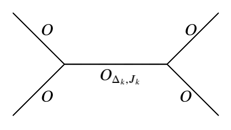
Figure 5: Schematic for the conformal block expansion

In the supersymmetric four point functions of $J_{0}$ operators, the relevant exchanges are schematically shown below

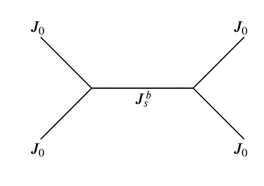
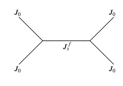
Figure 6: Schematic for the exchanges relevant in the supersymmetric scalar correlators

4.1 Review of the double discontinuity technique

In [51], the authors determine the four-point correlation functions of the scalar operator in the non-supersymmetric scalar/fermion coupled to Chern Simons gauge field i.e. quasi-bosonic and quasi-fermionic theory respectively. In order to obtain the required four-point functions, the authors utilize the inversion formula which relates the double discontinuity to the OPE coefficients [53]. The authors first prove an interesting theorem that in the large-N limit of a $CFT_{d}$, the double discontinuity constrains the four-point correlator up to three contact terms in $AdS_{d+1}$. Suppose there are two solutions $G_{1}$ and $G_{2}$ to the crossing equation with the same double discontinuity then they are related by the contact interactions in the AdS as follows

$$G_{1}=G_{2}+c_{1}G^{AdS}_{\phi^{4}}+c_{2}G^{AdS}_{(\partial\phi)^{4}}+c_{2}G^{AdS}_{\phi^{2}(\partial^{3}\phi)^{2}}$$ (4.3)

Furthermore, the authors showed that for the four-point function of single trace scalar operator in Chern-Simons coupled fundamental scalar/fermion theories these $AdS_{4}$ contact terms do not contribute and hence the double discontinuity completely determines the four-point functions.

Consider the normalized three point functions of the operators $\mathcal{O}_{i}$($i=1,2,3)$ which are defined as follows

$$C_{(123)}=\frac{\langle\mathcal{O}_{1}\mathcal{O}_{2}\mathcal{O}_{3}\rangle}{\sqrt{\langle\mathcal{O}_{1}\mathcal{O}_{1}\rangle\langle\mathcal{O}_{2}\mathcal{O}_{2}\rangle\langle\mathcal{O}_{3}\mathcal{O}_{3}\rangle}}.$$ (4.4)

In [3, 4, 51], it was noticed that the square of this normalized coefficients in the quasi-fermionic theories ($C^{2}_{s,qf}$) are related to that of a single free Majorana fermion ($C^{2}_{s,ff}$) as follows

$$C^{2}_{s,qf} = \frac{1}{\tilde{N}}C^{2}_{s,ff}$$ (4.5)

where $\tilde{N}$ is related to the the rank of the gauge group $N$ and coupling $\lambda_{qf}$ by,

$$\tilde{N}=2N\frac{\sin(\pi\lambda_{qf})}{\pi\lambda_{qf}}.$$ (4.6)

Note that the normalized coefficients of quasi-fermionic theory and free fermionic theory are proportional to each other as given in eq.(4.5). Hence, the double discontinuity of the scalar four point function in the free fermionic theory is same as that of the quasi-fermionic theories up to an overall factor which depends only on $N$ and $\lambda_{qf}$.

On the other hand, the square of the normalized coefficients of the quasi-bosonic theories ($C^{2}_{s,qb}$) are related to the theory of a free real boson ($C^{2}_{s,fb}$) as follows

$$C^{2}_{s,qb} = \frac{1}{\tilde{N}}C^{2}_{s,fb}~{}~{}~{}s>0,$$ (4.7)

$$C^{2}_{0,qb} = \frac{1}{\tilde{N}}\frac{1}{(1+\tilde{\lambda}_{qb}^{2})}C^{2}_{0,fb}=\frac{1}{\tilde{N}}C^{2}_{0,fb}-\frac{1}{\tilde{N}}\frac{\tilde{\lambda}_{qb}^{2}}{(1+\tilde{\lambda}_{qb}^{2})}C^{2}_{0,fb}.$$ (4.8)

where $\tilde{N}$ and $\tilde{\lambda}$ are related to $N$ and coupling $\lambda_{qb}$ as

$$\tilde{N}=2N\frac{\sin(\pi\lambda_{qb})}{\pi\lambda_{qb}},$$ (4.9)

$$\tilde{\lambda}_{qb}=\tan(\frac{\pi\lambda_{qb}}{2}).$$ (4.10)

Note that unlike the normalized coefficients of the quasi-fermionic theories, in the quasi-bosonic theories, the spin $s=0$ and $s\neq 0$ coefficients given above have different factors in front of their free bosonic counterparts. In order to account for the second term on the RHS of eq.(4.8) one needs to add a conformal partial wave with spin-0 exchange which is given by the well known $\bar{D}$-function with the correct pre-factor [51]. We now proceed to employ this technique for the supersymmetric case.

4.2 Double discontinuity and the supersymmetric correlators

Here, we utilize the technique described above to compute the four-point correlators for spin-$0$ operators $J^{b}_{0}$ and $J^{f}_{0}$ in our supersymmetric theory. Since we are considering correlators of identical external operators, only even spin operators will contribute to the block expansion.

4.2.1 $\langle J_{0}^{b}(x_{1})J_{0}^{b}(x_{2})J_{0}^{b}(x_{3})J_{0}^{b}(x_{4})\rangle$

The four point function of the $J_{0}^{b}$ operators is expressed as follows

$$\langle J_{0}^{b}(x_{1})J_{0}^{b}(x_{2})J_{0}^{b}(x_{3})J_{0}^{b}(x_{4})\rangle=disc+\frac{1}{x_{13}^{2}x_{24}^{2}}F(u,v).$$ (4.11)

Here, disc corresponds to the disconnected part given by

$$disc=\frac{1}{x_{12}^{2}x_{34}^{2}}+\frac{1}{x_{13}^{2}x_{24}^{2}}+\frac{1}{x_{14}^{2}x_{23}^{2}}$$ (4.12)

while $F(u,v)$ is given by

$$F(u,v)=\frac{1}{u}\sum_{k}C^{2}_{\mathcal{O}\mathcal{O}O_{k}}G_{\Delta_{k},J_{k}}(u,v)$$ (4.13)

In order to determine the double discontinuity, and hence the four-point functions in the supersymmetric case using the method described above, we first obtain all the normalized three-point functions coefficients defined in eq.(4.4). Utilizing the two and three point functions obtained in the previous section, the normalized coefficients for spins $s=0$ operators that contribute to the $J_{0}^{b}$ four point function are given as follows

$$C^{2(BBB)}_{0,susy} = \frac{1}{\tilde{N}}\frac{(1-\tilde{\lambda}^{2})^{2}}{(1+\tilde{\lambda}^{2})^{2}}~{}C^{2}_{0,fb,}$$ (4.14)

$$C^{2(BBF)}_{0,susy} = -\frac{4}{\tilde{N}}\frac{\tilde{\lambda}^{2}}{(1+\tilde{\lambda}^{2})^{2}}C^{2}_{0,fb}.$$ (4.15)

On the other hand the normalized coefficients involving one of operators with non-zero spin ($s>0$) are given by

$$C^{2(BBB)}_{s,susy}=\frac{1}{\tilde{N}(1+\tilde{\lambda}_{qb}^{2})^{2}}C^{2}_{s,fb}~{}~{}~{}~{}s>0,~{}~{}~{}\text{even}$$ (4.16)

$$\ C^{2(BBF)}_{s,susy}=\frac{\tilde{\lambda}_{qb}^{4}}{\tilde{N}(1+\tilde{\lambda}_{qb}^{2})^{2}}C^{2}_{s,fb}~{}~{}~{}~{}s>0,~{}~{}~{}\text{even},$$ (4.17)

where $C^{2}_{s,fb}$ is the corresponding normalized coefficient of three point function for the free bosonic theory. The derivations for the above relations are provided in the Appendix C.

Since, the above relations were computed in momentum-space, they must be converted to position-space to make our results useful.

$$\tilde{C}^{2(BBB)}_{0,susy} = \frac{1}{\tilde{N}}\frac{(1-\tilde{\lambda}_{qb}^{2})^{2}}{(1+\tilde{\lambda}_{qb}^{2})^{2}}~{}\tilde{C}^{2}_{0,fb,}$$ (4.18)

$$C^{2(BBF)}_{0,susy} = \frac{8}{\pi^{2}}\frac{\tilde{\lambda}_{qb}^{2}}{\tilde{N}(1+\tilde{\lambda}_{qb}^{2})^{2}}\tilde{C}^{2}_{0,fb}.$$ (4.19)

Similarly, for $s>0$ are given by

$$\tilde{C}^{2(BBB)}_{s,susy}=\frac{1}{\tilde{N}(1+\tilde{\lambda}_{qb}^{2})^{2}}\tilde{C}^{2}_{s,fb}~{}~{}~{}~{}s>0,$$ (4.20)

$$\ \tilde{C}^{2(BBF)}_{s,susy}=\frac{\tilde{\lambda}_{qb}^{4}}{\tilde{N}(1+\tilde{\lambda}_{qb}^{2})^{2}}\tilde{C}^{2}_{s,fb}~{}~{}~{}~{}s>0,$$ (4.21)

Note that we may re-express both the spin zero coefficients given by eq.(4.18) and eq.(4.19) as follows

$$\tilde{C}^{2(BBB)}_{0,susy} = \frac{1}{\tilde{N}(1+\tilde{\lambda}_{qb}^{2})^{2}}\tilde{C}^{2}_{0,fb}+\frac{\tilde{\lambda}_{qb}^{4}-2\tilde{\lambda}_{qb}^{2}}{\tilde{N}(1+\tilde{\lambda}_{qb}^{2})^{2}}\tilde{C}^{2}_{0,fb},$$ (4.22)

Observe that $\tilde{C}^{2(BBB)}_{s,susy}$ in eq.(4.20) and the first term of $\tilde{C}^{2(BBB)}_{0,susy}$ in (4.22) have the same pre-factor. This is similar to the case of the quasibosnic case given in eq.(4.7) and eq.(4.8) reviewed earlier. Consider, now, the double discontinuity of the conformal blocks

$$\text{dDisc}[G_{\Delta,J}(1-z,1-\bar{z})]=\sin^{2}(\frac{\pi}{2}(\Delta-J-2\Delta_{\phi}))G_{\Delta,J}(1-z,1-\bar{z})$$ (4.23)

where $\Delta_{\phi}$ being the conformal dimension of the external operator. Notice that for $\Delta=2\Delta_{\phi}+J+2m$, the double-discontinuity vanishes. Therefore, for the double-trace exchange, the double-discontinuity vanishes. That is why the OPE of single-trace operators are sufficient to construct a function that has a double-discontinutiy equal to the four-point correlator. However, notice that the single-trace exchange $J^{FF}_{0}$ with quantum numbers $(\Delta,J)=(2,0)$ also vanish. Coincidently, the double-trace operator $[J^{b}_{0},J^{b}_{0}]_{0,0}$ also has the same quantum numbers. By inspection, we can see that the function below has the right double-discontinuity

$$F(u,v) =\frac{1+\tilde{\lambda}_{qb}^{4}}{\tilde{N}(1+\tilde{\lambda}_{qb}^{2})^{2}}f_{fb}(u,v)-\frac{8}{\tilde{N}}\frac{2\tilde{\lambda}_{qb}^{2}}{\pi^{5/2}(1+\tilde{\lambda}_{qb}^{2})^{2}}\big{[}\bar{D}_{11\frac{1}{2}\frac{1}{2}}(u,v)+\bar{D}_{11\frac{1}{2}\frac{1}{2}}(v,u)+\frac{1}{u}\bar{D}_{11\frac{1}{2}\frac{1}{2}}(\frac{1}{u},\frac{v}{u})\big{]}$$

$$+c_{1}G^{AdS}_{\phi^{4}}+c_{2}G^{AdS}_{(\partial\phi)^{4}}+c_{3}G^{AdS}_{\phi^{2}(\partial^{3}\phi)^{2}}$$ (4.24)

where, the function $f_{fb}(u,v)$ is the free bosonic part given by.

$$f_{fb}(u,v)=4\frac{1+u^{1/2}+v^{1/2}}{u^{1/2}v^{1/2}}$$ (4.25)

The contact terms are explicitly provided in E.18. Note that $c_{1}$ contains contribution from both single-trace and double-trace operators which we have separated in the following equation as $a_{1}$ and $\tilde{c}_{1}$

$$F(u,v) =\frac{1+\tilde{\lambda}_{qb}^{4}}{\tilde{N}(1+\tilde{\lambda}_{qb}^{2})^{2}}f_{fb}(u,v)-\frac{8}{\tilde{N}}\frac{2\tilde{\lambda}_{qb}^{2}}{\pi^{5/2}(1+\tilde{\lambda}_{qb}^{2})^{2}}\big{[}\bar{D}_{11\frac{1}{2}\frac{1}{2}}(u,v)+\bar{D}_{11\frac{1}{2}\frac{1}{2}}(v,u)+\frac{1}{u}\bar{D}_{11\frac{1}{2}\frac{1}{2}}(\frac{1}{u},\frac{v}{u})\big{]}$$

$$+a_{1}\bar{D}_{1111}(u,v)+\tilde{c}_{1}G^{AdS}_{\phi^{4}}+c_{2}G^{AdS}_{(\partial\phi)^{4}}+c_{3}G^{AdS}_{\phi^{2}(\partial^{3}\phi)^{2}}$$ (4.26)

To determine $a_{1}$ we take the OPE limit. In the OPE limit, the conformal blocks go like

$$G_{\Delta,J}(u,v)\approx\frac{J!}{2^{J}(h-1)_{J}}u^{\Delta/2}C^{h-1}_{J}(\frac{v-1}{2\sqrt{u}})$$ (4.27)

For $(\Delta,J)=(2,0)$ i.e. for $J^{f}_{0}$ exchange, we have $G_{2,0}(u,v)\approx u$ in the OPE limit. Since, we are interested in the single-trace operator $J^{f}_{0}$, hence, we have

$$F(u,v)=\tilde{C}^{2(BBF)}_{0,susy}$$ (4.28)

In the OPE limit, we have for $\phi^{4}$ contact term

$$\bar{D}_{1111}(u,v)\approx 2$$ (4.29)

By only looking at the single-trace contributions we obtain

$$a_{1}=\frac{\tilde{C}^{2(BBF)}_{0,susy}}{2}$$ (4.30)

Now, we focus our attention to double-trace operators. Coefficient $\tilde{c}_{1}$ can now be determined by looking at the double-trace trace operator $[J^{b}_{0},J^{b}_{0}]_{0,0}$. Since, $(\Delta,J)=(2,0)$ for the double-trace is same as that of the single-trace operator $J^{f}_{0}$, we use the same method to obtain $\tilde{c}_{1}$

Hence, we have determined the first coefficient of the AdS contact terms. The results are a little cumbersome and we report it in the appendix F. We leave the explicit computation of these ope coefficients for future work.

$$\bar{c}_{1}=\frac{1}{2}\bigg{(}[\tilde{C}^{2(FFF)}_{0,susy}]_{[O,O]_{0,0}}-\frac{1}{\tilde{N}}\frac{4\tilde{\lambda}_{qb}^{2}}{(1+\tilde{\lambda}_{qb}^{2})^{2}\pi^{2}}\tilde{C}^{2}_{0,fb}-\frac{1+\tilde{\lambda}_{qb}^{4}}{\tilde{N}(1+\tilde{\lambda}_{qb}^{2})^{2}}[\tilde{C}^{2}_{0,fb}]_{[O,O]_{0,0}}\bigg{)}$$ (4.31)

4.2.2 $\langle J_{0}^{f}(x_{1})J_{0}^{f}(x_{2})J_{0}^{f}(x_{3})J_{0}^{f}(x_{4})\rangle$

The four point function of $J_{0}^{f}$ is given by the following expression

$$\langle J_{0}^{f}(x_{1})J_{0}^{f}(x_{2})J_{0}^{f}(x_{3})J_{0}^{f}(x_{4})\rangle=disc+\frac{1}{x_{13}^{4}x_{24}^{4}}\mathcal{G}(u,v)$$ (4.32)

where, $disc$ denotes the disconnected piece given by

$$disc=\frac{1}{x_{12}^{4}x_{34}^{4}}+\frac{1}{x_{13}^{4}x_{24}^{4}}+\frac{1}{x_{14}^{4}x_{23}^{4}}$$ (4.33)

while $F(u,v)$ is given by

$$\mathcal{G}(u,v)=\frac{1}{u}\sum_{k}C^{2}_{\mathcal{O}\mathcal{O}O_{k}}G_{\Delta_{k},J_{k}}(u,v)$$ (4.34)

We now proceed to determine the four-point function $J_{0}^{f}$ utilizing the same technique. The normalized coefficients that are required in this case are given by

$$C^{2(FFF)}_{s,susy}=\frac{\tilde{\lambda}_{qf}^{4}}{\tilde{N}(1+\tilde{\lambda}_{qf}^{2})^{2}}C^{2}_{s,ff},$$ (4.35)

$$C^{2(FFB)}_{s,susy}=\frac{1}{\tilde{N}(1+\tilde{\lambda}_{qf}^{2})^{2}}C^{2}_{s,ff},$$ (4.36)

where $C^{2}_{s,ff}$ is the normalized three point functions for free fermionic theory. Unlike the previous section, changing the OPE coefficients to position-space is redundant here as both sides of the eqaution change by the same factor. Once again these relations are derived in Appendix C. Note that the three point functions of the spin-0 exchanges given by $C^{2(FFF)}_{0,susy}$ and $C^{2(FFB)}_{0,susy}$ are contact terms in this case which, therefore, may be set to zero. This implies that the above relation is trivially satisfied for the spin $s=0$ case as the free fermionic coeffcient $C^{2}_{0,ff}=0$. Hence, both the $s=0$ and $s\neq 0$ coefficients in this case come with the same pre-factor. This implies that the function which has the correct double discontinuity is given by

$$\mathcal{G}(u,v)=\frac{1+\tilde{\lambda}_{qf}^{4}}{\tilde{N}(1+\tilde{\lambda}_{qf}^{2})^{2}}f_{ff}(u,v)+\bar{c}_{1}G^{AdS}_{\phi^{4}}+\bar{c}_{2}G^{AdS}_{(\partial\phi)^{4}}+\bar{c}_{3}G^{AdS}_{\phi^{2}(\partial^{3}\phi)^{2}},$$ (4.37)

where $f_{ff}(u,v)$ is the free fermionic part given by

$$f_{ff}(u,v)=\frac{1+u^{5/2}+v^{5/2}-u^{3/2}(1+v)-v^{3/2}(1+u)-u-v}{u^{3/2}v^{3/2}}$$ (4.38)

However, in this case, the separation of the double-trace and the single trace contributions is redundant as there are no single-trace operators with $(\Delta,J)=(4,0)$. After a faithful implementation of the methodology of the previous section, we obtain

$$\bar{c}_{1}=\frac{3\pi^{1/2}}{8P^{(2)}_{1}(0,0)}\bigg{(}[\tilde{C}^{2(FFF)}_{0,susy}]_{[O,O]_{0,0}}-\frac{1+\tilde{\lambda}^{4}}{\tilde{N}(1+\tilde{\lambda}^{2})^{2}}[\tilde{C}^{2}_{0,ff}]_{[O,O]_{0,0}}\bigg{)}$$ (4.39)

This completes our analysis of the determination of the four point functions of $J_{0}^{b}$ and $J_{0}^{f}$ operators in the Chern Simons matter theories in the supersymmetric scenario. The contact terms are explicitly provided in E.19. The results are a little cumbersome and we report it in the appendix F. We leave the explicit computation of these ope coefficients for future work.

5 Summary and Discussion

In this article, we have focused our attention on the ${\cal N}=2$ $U(N)$ Chern Simons theory coupled with a single fundamental chiral multiplet in the ’t Hooft large $N$ limit and presented the computations for the exact 2 and 3-point functions for the scalar supermultiplet. The result are invariant the duality transformation (2.3) and can be seen as an independent confirmation of the duality. For the case of 4-point function, though we are not able to perform the direct computation for the full scalar supermultiplet, we are able to use the a combination of techniques from conformal bootstrap, factorization of 3-point functions via double trace interactions along with the self duality of our theory to write down two of the component of the full $J_{0}$ 4-point function. Though this leave room for 3 undetermined coefficient, we could formally related these to 3 point function coefficients involving specific double trace operators. We plan to report on these in near future.

Though we have focused on the ${\cal N}=2$ theory in this paper, the approach used to compute the four point function is can be straightforwardly applied to the one parameter deformed ${\cal N}=1$ theory. These differ from our ${\cal N}=2$ theory only via a double trace term in ${\cal N}=1$ superspace. The 2 and 3-point functions of the two theories can thus be related via the double trace type factorization also used in this paper.

The approach used in this paper, following [51], to compute the $J_{0}^{b}$ and $J_{0}^{f}$ 4-point functions relies crucially on the fact that the double discontinuity of the 4-point function in the interacting theory is almost the same as that of the free theory. We could thus write down the full interacting 4-point function in term of the free 4-point function. For the case of mixed 4-point functions, e.g. $\langle J_{0}^{b}J_{0}^{b}J_{0}^{f}J_{0}^{f}\rangle$, this approach is not directly useful since a free theory analogue of such mixed correlator is not available since bosons and fermions decouple from each other the mixed 4 point correlators vanish in $\lambda\rightarrow 0$ limit. One approach that might be useful in this regard is to first study the single trace OPE coefficients in the ${\cal N}=1$ deformed theory (for general $w$) in $\lambda=0$ limit. We expect this limit to be significantly simpler then ${\cal N}=2$ theory and one can compute not only the exact 2, 3 point functions (see e.g. [54]) but perhaps even the exact 4-point function (we expect it to be non vanishing for $w\neq 0$) of $J_{0}$ operators in this limit since the only interaction term present is a double trace term. If this is indeed turn out to be the case, one can compare the double discontinuity of mixed $J_{0}^{b},J_{0}^{f}$ correlators in ${\cal N}=2$ theory with this limit and see these are closely related in a similar way as in [51] and in this paper for the identical scalar 4-point function.

As we have noticed in this paper, the coefficients $\{c_{i}\}$ can be determined in term of the normalized 3-point function coefficients of specific double trace operator. An interesting property of the $AdS_{4}$ contact Witten diagrams is that their series expansions contain $Log$ terms. This implies that the coefficients $\{c_{i}\}$ not only contribute to the OPE coefficients of double trace terms but also to their leading anomalous dimensions as well, but in a coordinated way. The absence of $Log$ term in the free 4-point function along with the vanishing of these coefficients for quasi-bosonic and quasi-fermionic theories [51] thus means that these double trace operators in the leading large-N order do not receive corrections to there anomalous dimensions these theories. Whether this is also the case in the supersymmetric theory studied in this paper as well requires the computation of anomalous dimensions of these double trace operators which we leave for future investigation.

Appendix A Notations and Conventions

$$\begin{split}\textrm{Metric}&:\eta_{\mu\nu}=\textrm{diag}(-1,1,1)\\ \textrm{Gamma Matrices}&:(\gamma^{\mu})_{\alpha}^{~{}\beta}=(\sigma_{2},-i\sigma_{1},i\sigma_{3})_{\alpha}^{~{}\beta}\quad\Rightarrow\{\gamma^{\mu},\gamma^{\nu}\}=-2\eta^{\mu\nu}I_{2}\\ \textrm{Charge Conjugation}&:C_{\alpha\beta}=-C_{\beta\alpha}=\begin{pmatrix}0&-i\\ i&0\end{pmatrix}=-C^{\alpha\beta}=C^{\beta\alpha}\\ \textrm{Raising-Lowering}&:\psi^{\alpha}=C^{\alpha\beta}\psi_{\beta}\quad;\quad\psi_{\alpha}=-C_{\alpha\beta}\psi^{\beta}=\psi^{\beta}C_{\beta\alpha}\\ &\Rightarrow\psi^{+}=i\psi_{-}\quad;\quad\psi^{-}=-i\psi_{+}\\ \textrm{Vector $\leftrightarrow$ Bi-spinor}&:p_{\alpha\beta}=p_{\mu}(\gamma^{\mu})_{\alpha\beta}=\begin{pmatrix}p_{0}+p_{1}&p_{3}\\ p_{3}&p_{0}-p_{1}\end{pmatrix}=\begin{pmatrix}p_{+}&p_{3}\\ p_{3}&-p_{-}\end{pmatrix}\\ \textrm{Squared Grassmann variables }&:\theta^{2}=\frac{1}{2}\theta^{\alpha}\theta_{\alpha},\ d^{2}\theta=\frac{1}{2}d\theta^{\alpha}d\theta_{\alpha}\\ \textrm{Superspace integrals }&:\int d\theta=0,\ \int d\theta\ \theta=1\\ &\int d^{2}\theta\ \theta^{2}=-1,\ \int d^{2}\theta\ \theta^{\alpha}\theta^{\beta}=C^{\alpha\beta}\\ \textrm{Grassmann $\delta$-function }&:\delta^{2}(\theta)=-\theta^{2}\\ \textrm{Superfields }&:\Phi=\phi+\theta\psi-\theta^{2}F,\ \bar{\Phi}=\bar{\phi}+\theta\bar{\psi}-\theta^{2}\bar{F}\\ &\bar{\Phi}\Phi=\bar{\phi}\phi+\theta^{\alpha}\left(\bar{\phi}\psi_{\alpha}+\bar{\psi}_{\alpha}\phi\right)-\theta^{2}\left(\bar{F}\phi+\bar{\phi}F+\bar{\psi}\psi\right)\end{split}$$ (A.1)

Appendix B Component 3 point functions

In this appendix, we write down the component 3 functions abstractly in term of the functions $\{A_{i}\}$ appearing in form of full superspace 3 point function (LABEL:J03ptresult) determined by supersymmetric Ward identity.

$$\begin{split}\langle J^{b}_{0}(p)J^{b}_{0}(-p-s)J^{b}_{0}(s)\rangle&=2A_{1}\\ \langle J^{f}_{0}(p)J^{f}_{0}(-p-s)J^{f}_{0}(s)\rangle&=2(A_{3}p_{3}^{2}+s_{3}(-A_{4}p_{3}-A_{5}p_{3}+A_{2}s_{3}))\\ \langle J^{b}_{0}(p)J^{f}_{0}(-p-s)J^{b}_{0}(s)\rangle&=2(A_{2}+A_{3}+A_{4}+A_{5})\\ \langle J^{f}_{0}(p)J^{b}_{0}(-p-s)J^{f}_{0}(s)\rangle&=\frac{2}{9}(9A_{6}+(p_{3}-s_{3})(3A_{4}-3A_{5}+A_{1}p_{3}-A_{1}s_{3}))\\ \langle\Psi_{+}(p)J^{b}_{0}(-p-s)\Psi_{-}(s)\rangle&=-\frac{2}{3}(3A_{5}+A_{1}(-p_{3}+s_{3}))\\ \langle\Psi_{+}(p)J^{b}_{0}(-p-s)\Psi_{-}(s)\rangle&=-\frac{2}{9}(-9A_{6}+p_{3}(-3(3A_{3}+A_{4}+2A_{5})+2A_{1}p_{3})\\ &\qquad+(9A_{2}+3A_{4}+6A_{5}+5A_{1}p_{3})s_{3}+2A_{1}s_{3}^{2})\end{split}$$ (B.1)

Appendix C Normalized higher spin three point functions

In this section, we aim to derive the normalized coefficients of the three point functions involving two $J_{0}$ operators and one higher spin operator $J_{s}$ ($s>1$) leading to eq.(4.16), (4.17), (4.35) and (4.36). The classical action for ${\cal N}=2$ supersymmetric matter coupled to Chern Simons gauge field is given by

$$S^{\mathcal{T}}_{k,N}=\frac{ik}{4\pi}S_{CS}(A)+S_{\mathcal{B}_{k,N}}(A,\phi)+S_{\mathcal{F}_{k,N}}(A,\psi)+S_{bf}(\varphi,\psi)$$

$$S_{CS}(A)=\int d^{3}x~{}\epsilon_{\mu\nu\rho}\text{Tr}(A^{\mu}\partial^{\nu}A^{\rho}-\frac{2i}{3}A^{\mu}A^{\nu}A^{\rho})$$

$$S_{\mathcal{B}_{k,N}}(A,\phi)=\frac{ik}{4\pi}S_{CS}(A)+\mathcal{D}_{\mu}\bar{\varphi}\mathcal{D}^{\mu}\varphi$$

$$S_{\mathcal{F}_{k,N}}(A,\psi)=\frac{ik}{4\pi}S_{CS}(A)-i\bar{\psi}\gamma^{\mu}\mathcal{D}_{\mu}\psi$$ (C.1)

$$S_{bf}(\varphi,\psi)=\int d^{3}x[-\frac{4\pi i}{k}(\bar{\varphi}\varphi)(\bar{\psi}\psi)+\frac{4\pi^{2}}{k^{2}}(\bar{\varphi}\varphi)^{3}-\frac{2\pi i}{k}(\bar{\psi}\varphi)(\bar{\varphi}\psi)]$$

Note that we will be using the following notation for correlation functions in the superymmetric and the non-supersymmetric theories

$$\langle\cdots\rangle_{\mathcal{T}_{k,N}}~{}~{}~{}~{}~{}~{}~{}\text{Correlator in SUSY theory}$$

$$\langle\cdots\rangle_{\mathcal{B}_{k,N}}~{}~{}~{}~{}~{}~{}~{}\text{Correlator in regular bosonic theory}$$

$$\langle\cdots\rangle_{\mathcal{F}_{k,N}}~{}~{}~{}~{}~{}~{}~{}\text{Correlator in regular fermionic theory}$$

$$\langle\cdots\rangle_{fb}~{}~{}~{}~{}~{}~{}~{}~{}~{}~{}\text{Correlator in free bosonic theory}$$

$$\langle\cdots\rangle_{ff}~{}~{}~{}~{}~{}~{}~{}~{}~{}~{}\text{Correlator in free fermionic theory}$$

We begin with the derivation of relation between the normalized three point functions of the $\langle J_{s}^{b}J_{0}^{b}J_{0}^{b}\rangle$ in supersymmetric theory and the corresponding three point function in the free bosonic theory. We will employ the path integral technique and utilize some of the relations derived in [20]. The correlation function $\langle J_{s}^{b}J_{0}^{b}J_{0}^{b}\rangle_{\mathcal{T}_{k,N}}$ in the path integral representation may be expressed as follows

$$\langle J_{s}^{b}(x_{a})J_{0}^{b}(x_{b})J_{0}^{b}(x_{c})\rangle_{\mathcal{T}_{k,N}}$$

$$=\int\mathcal{D}\phi~{}J_{s}^{b}(x_{a})J_{0}^{b}(x_{b})J_{0}^{b}(x_{c})~{}e^{-S^{\mathcal{B}}_{k,N}-S^{\mathcal{F}}_{k,N}}(1-S_{bf}+\frac{1}{2!}S^{2}_{bf}-\frac{1}{3!}S^{3}_{bf}+\cdots)$$

$$=\langle J_{s}^{b}(x_{a})J_{0}^{b}(x_{b})J_{0}^{b}(x_{c})\rangle_{\mathcal{B}_{k,N}}$$

$$-\frac{4\pi}{k}\int_{1}\langle J_{s}^{b}(x_{a})J_{0}^{b}(x_{b})J_{0}^{b}(x_{c})J_{0}^{b}(x_{1})\rangle_{\mathcal{B}_{k,N}}\langle J_{0}^{f}(x_{1})\rangle_{\mathcal{F}_{k,N}}$$

$$+\frac{1}{2!}(\frac{4\pi}{k})^{2}\int_{12}\langle J_{s}^{b}(x_{a})J_{0}^{b}(x_{b})J_{0}^{b}(x_{c})J_{0}^{b}(x_{1})J_{0}^{b}(x_{2})\rangle_{\mathcal{B}_{k,N}}\langle J_{0}^{f}(x_{1})J_{0}^{f}(x_{2})\rangle_{\mathcal{F}_{k,N}}$$

$$-\frac{1}{3!}(\frac{4\pi}{k})^{3}\int_{123}\langle J_{s}^{b}(x_{a})J_{0}^{b}(x_{b})J_{0}^{b}(x_{c})J_{0}^{b}(x_{1})J_{0}^{b}(x_{2})J_{0}^{b}(x_{3})\rangle_{\mathcal{B}_{k,N}}\langle J_{0}^{f}(x_{1})J_{0}^{f}(x_{2})J_{0}^{f}(x_{3})\rangle_{\mathcal{F}_{k,N}}+\cdots$$ (C.3)

In the first line, we have implemented factorization of planar correlators through the multi-trace interactions of the SUSY theory by splitting the action into non-SUSY components[20]. Now, by usual arguments of connectedness and by Wick’s theorem,

$$\langle J_{s}^{b}(x_{a})J_{0}^{b}(x_{b})J_{0}^{b}(x_{c})\rangle_{\mathcal{T}_{k,N}}$$

$$=\langle J_{s}^{b}(x_{a})J_{0}^{b}(x_{b})J_{0}^{b}(x_{c})\rangle_{\mathcal{B}_{k,N}}+2(\frac{4\pi}{k})^{2}\int_{12}\langle J_{0}^{b}J_{0}^{b}(x_{1})\rangle_{\mathcal{B}_{k,N}}\langle J^{b}_{s}J_{0}^{b}J_{0}^{b}(x_{2})\rangle_{\mathcal{B}_{k,N}}\langle J_{0}^{f}(x_{1})J_{0}^{f}(x_{2})\rangle_{\mathcal{F}_{k,N}}+\cdots$$

$$=\langle J_{s}^{b}(x_{a})J_{0}^{b}(x_{b})J_{0}^{b}(x_{c})\rangle_{\mathcal{B}_{k,N}}(1+\sum_{n=1}^{\infty}(n+1)[(\frac{4\pi}{k})^{2}\langle J_{0}^{b}J_{0}^{b}\rangle_{\mathcal{B}_{k,N}}\langle J_{0}^{f}J_{0}^{f}\rangle_{\mathcal{F}_{k,N}}]^{n})$$

$$=\langle J_{s}^{b}(x_{a})J_{0}^{b}(x_{b})J_{0}^{b}(x_{c})\rangle_{\mathcal{B}_{k,N}}\frac{1}{(1-(\frac{4\pi}{k})^{2}\langle J_{0}^{b}J_{0}^{b}\rangle_{\mathcal{B}_{k,N}}\langle J_{0}^{f}J_{0}^{f}\rangle_{\mathcal{F}_{k,N}})^{2}}$$ (C.4)

The various integrations and the position labels in the above are implicit. The implicit notation and the momentum space representation are look identical and therefore, the implicit format may be viewed in momentum-space representation. In eq.(20) of [20], an interesting relation was derived between the two point function which is given as

$$\langle J_{0}^{b}J_{0}^{f}\rangle_{\mathcal{T}_{k,N}}=-\frac{k}{4\pi}\sum_{n=1}^{\infty}(\frac{4\pi}{k})^{2}\langle J_{0}^{b}J_{0}^{b}\rangle_{\mathcal{B}_{k,N}}\langle J_{0}^{f}J_{0}^{f}\rangle_{\mathcal{F}_{k,N}}$$ (C.5)

Hence eq.(C.4) simplifies upon utilizing the above relation as

$$\langle J_{s}^{b}(x_{a})J_{0}^{b}(x_{b})J_{0}^{b}(x_{c})\rangle_{\mathcal{T}_{k,N}} =\langle J_{s}^{b}(x_{a})J_{0}^{b}(x_{b})J_{0}^{b}(x_{c})\rangle_{\mathcal{B}_{k,N}}[1-\frac{4\pi}{k}\langle J_{0}^{b}J_{0}^{f}\rangle_{\mathcal{T}_{k,N}}]^{2}$$

$$=\langle J_{s}^{b}(x_{a})J_{0}^{b}(x_{b})J_{0}^{b}(x_{c})\rangle_{\mathcal{B}_{k,N}}\frac{1}{(1+\tilde{\lambda}^{2})^{2}}$$ (C.6)

Note that in order to arrive at the last line in the above relation we have utilized the explicit form of the two point function $\langle J_{0}^{b}J_{0}^{f}\rangle_{\mathcal{T}_{k,N}}$ which we had derived earlier. The two point functions in the supersymmetric theory are related to the regular bosonic theory as follows [20]

$$\langle J_{s}^{b}J_{s}^{b}\rangle_{\mathcal{T}_{k,N}} = \langle J_{s}^{b}J_{s}^{b}\rangle_{\mathcal{B}_{k,N}}$$ (C.7)

$$\langle J_{0}^{b}J_{0}^{b}\rangle_{\mathcal{T}_{k,N}} = \langle J_{0}^{b}J_{0}^{b}\rangle_{\mathcal{B}_{k,N}}[1-\frac{4\pi}{k}\langle J_{0}^{b}J_{0}^{f}\rangle_{\mathcal{T}_{k,N}}]$$ (C.8)

From eq.(C.6), eq.(C.7) and eq.(C.8) we obtain the normalized coefficients as

$$\frac{\langle J_{s}^{b}J_{0}^{b}J_{0}^{b}\rangle_{\mathcal{T}_{k_{e},N_{e}}}}{\langle J_{0}^{b}J_{0}^{b}\rangle_{\mathcal{T}_{k_{e},N_{e}}}\sqrt{\langle J_{s}^{b}J_{s}^{b}\rangle_{\mathcal{T}_{k_{e},N_{e}}}}}=\frac{1}{\sqrt{\tilde{N}}(1+\tilde{\lambda}^{2})}\frac{\langle J_{s}^{b}J_{0}^{b}J_{0}^{b}\rangle_{fb}}{\langle J_{0}^{b}J_{0}^{b}\rangle_{fb}\sqrt{\langle J_{s}^{b}J_{s}^{b}\rangle_{fb}}}$$ (C.9)

where, we have made use of the relation between the normalized coefficients of the regular bosonic theory and the free bosonic theory derived in [3, 4]

$$\frac{\langle J_{s}^{b}J_{0}^{b}J_{0}^{b}\rangle_{\mathcal{B}_{k_{e},N_{e}}}}{\langle J_{0}^{b}J_{0}^{b}\rangle_{\mathcal{B}_{k_{e},N_{e}}}\sqrt{\langle J_{s}^{b}J_{s}^{b}\rangle_{\mathcal{B}_{k_{e},N_{e}}}}}=\frac{1}{\sqrt{\tilde{N}}}\frac{\langle J_{s}^{b}J_{0}^{b}J_{0}^{b}\rangle_{fb}}{\langle J_{0}^{b}J_{0}^{b}\rangle_{fb}\sqrt{\langle J_{s}^{b}J_{s}^{b}\rangle_{fb}}}$$ (C.10)

Thus, from eq.(C.9) we have obtained the required relation

$$C^{2(BBB)}_{s,susy}=\frac{1}{\tilde{N}(1+\tilde{\lambda}_{qb}^{2})^{2}}C^{2}_{s,fb}$$ (C.11)

where

$$\tilde{\lambda}_{qb}=\tilde{\lambda}=\tan(\frac{\pi\lambda}{2})$$ (C.12)

A similar calculation allows one to write

$$\langle J_{s}^{f}(x_{a})J_{0}^{f}(x_{b})J_{0}^{f}(x_{c})\rangle_{\mathcal{T}_{k,N}}=\langle J_{s}^{f}(x_{a})J_{0}^{f}(x_{b})J_{0}^{f}(x_{c})\rangle_{\mathcal{F}_{k,N}}[1-\frac{4\pi}{k}\langle J_{0}^{b}J_{0}^{f}\rangle_{\mathcal{T}_{k,N}}]^{2}$$ (C.13)

Upon using the two point functions leads to the normalized coefficient

$$\frac{\langle J_{s}^{f}J_{0}^{f}J_{0}^{f}\rangle_{\mathcal{T}_{k_{e},N_{e}}}}{\langle J_{0}^{f}J_{0}^{f}\rangle_{\mathcal{T}_{k_{e},N_{e}}}\sqrt{\langle J_{s}^{f}J_{s}^{f}\rangle_{\mathcal{T}_{k_{e},N_{e}}}}}=\frac{1}{\sqrt{\tilde{N}}(1+\tilde{\lambda}^{2})}\frac{\langle J_{s}^{f}J_{0}^{f}J_{0}^{f}\rangle_{ff}}{\langle J_{0}^{f}J_{0}^{f}\rangle_{ff}\sqrt{\langle J_{s}^{f}J_{s}^{f}\rangle_{ff}}}$$ (C.14)

Hence we obtain the required coefficient as

$$C^{2(FFF)}_{s,susy}=\frac{1}{\tilde{N}(1+\tilde{\lambda}_{qb}^{2})^{2}}C^{2}_{s,ff}=\frac{\tilde{\lambda}_{qf}^{4}}{\tilde{N}(1+\tilde{\lambda}_{qf}^{2})^{2}}C^{2}_{s,ff}$$ (C.15)

where

$$\tilde{\lambda}_{qf}=\frac{1}{\tilde{\lambda}}=\cot(\frac{\pi\lambda}{2})$$ (C.16)

In order to derive the other two coefficients in eq.(4.17) and eq.(4.36), we make use of the Giveon-Kutasov duality which relates the magnetic theory to the electric counterpart through the following exchanges[37, 34, 20]

$$J_{0}^{f}\leftrightarrow-J_{0}^{f}~{}~{}J_{0}^{b}\leftrightarrow-J_{0}^{b}~{}~{}J_{s}^{f}\leftrightarrow(-1)^{s}J_{s}^{b}$$ (C.17)

to write the following

$$\langle J_{s}^{f}J_{0}^{f}J_{0}^{f}\rangle_{\mathcal{T}_{k_{e},N_{e}}}=(-1)^{s}\langle J_{s}^{b}J_{0}^{f}J_{0}^{f}\rangle_{\mathcal{T}_{k_{m},N_{m}}}$$ (C.18)

$$\langle J_{s}^{b}J_{0}^{b}J_{0}^{b}\rangle_{\mathcal{T}_{k_{e},N_{e}}}=(-1)^{s}\langle J_{s}^{f}J_{0}^{b}J_{0}^{b}\rangle_{\mathcal{T}_{k_{m},N_{m}}}$$ (C.19)

where now the labels $(k_{e},N_{e})$ and $(k_{m},N_{m})$ represent the electric $(e)$ and the magnetic $(m)$ theories, respectively. Now, by the normalization convention of (7), we can rewrite the following,

$$\frac{\langle J_{s}^{b}J_{0}^{f}J_{0}^{f}\rangle_{\mathcal{T}_{k_{e},N_{e}}}}{\langle J_{0}^{f}J_{0}^{f}\rangle_{{\cal T}_{k_{e},N_{e}}}\sqrt{\langle J_{0}^{f}J_{0}^{f}\rangle}_{\mathcal{T}_{k_{e},N_{e}}}} =(-1)^{s}\frac{\langle J_{s}^{f}J_{0}^{f}J_{0}^{f}\rangle_{\mathcal{T}_{k_{m},N_{m}}}}{\langle J_{0}^{f}J_{0}^{f}\rangle_{{\cal T}_{k_{m},N_{m}}}\sqrt{\langle J_{s}^{f}J_{s}^{f}\rangle_{{\cal T}_{k_{m},N_{m}}}}}$$ (C.20)

$$=\frac{1}{(1+\tilde{\lambda}_{m}^{2})}\frac{\langle J_{s}^{f}J_{0}^{f}J_{0}^{f}\rangle_{\mathcal{F}_{k_{m},N_{m}}}}{\langle J_{0}^{f}J_{0}^{f}\rangle_{\mathcal{F}_{k_{m},N_{m}}}\sqrt{\langle J_{s}^{f}J_{s}^{f}\rangle_{\mathcal{F}_{k_{m},N_{m}}}}}$$

$$=\frac{\tilde{\lambda}_{e}^{2}}{\sqrt{\tilde{N}_{e}}(1+\tilde{\lambda}_{e}^{2})}\frac{\langle J_{s}^{f}J_{0}^{f}J_{0}^{f}\rangle_{ff}}{\langle J_{0}^{f}J_{0}^{f}\rangle_{ff}\sqrt{\langle J_{s}^{f}J_{s}^{f}\rangle_{ff}}}$$ (C.21)

The first equality uses the duality described in eq.(C.17). The second equality makes use of the relation derived in eq.(C.14). The third equality utilizes the results of Maldacena and Zhiboedov derived in [3, 4] and the relation between the parameters of the magnetic and electric theory namely $\tilde{N}_{m}=\tilde{N}_{e}$ and $\tilde{\lambda}_{m}=\frac{1}{\tilde{\lambda}_{e}}$. This leads to the following expression for the normalized coefficient

$$C^{2(FFB)}_{s,susy}=\frac{\tilde{\lambda}^{4}}{\tilde{N}(1+\tilde{\lambda}^{2})^{2}}C^{2}_{s,ff}=\frac{1}{\tilde{N}(1+\tilde{\lambda}_{qf}^{2})^{2}}C^{2}_{s,ff}$$ (C.22)

Similar computations allow us to write

$$\frac{\langle J_{s}^{f}J_{0}^{b}J_{0}^{b}\rangle_{\mathcal{T}_{k_{e},N_{e}}}}{\langle J_{0}^{b}J_{0}^{b}\rangle_{{\cal T}_{k_{e},N_{e}}}\sqrt{\langle J_{s}^{f}J_{s}^{f}\rangle_{\mathcal{T}_{k_{e},N_{e}}}}} =(-1)^{s}\frac{\langle J^{b}_{s}J_{0}^{b}J_{0}^{b}\rangle_{\mathcal{T}_{k_{m},N_{m}}}}{\langle J_{0}^{b}J_{0}^{b}\rangle_{{\cal T}_{k_{m},N_{m}}}\sqrt{\langle J_{s}^{b}J_{s}^{b}\rangle_{{\cal T}_{k_{m},N_{m}}}}}$$ (C.23)

$$=\frac{1}{1+\tilde{\lambda}_{m}^{2}}\frac{\langle J_{s}^{b}J_{0}^{b}J_{0}^{b}\rangle_{\mathcal{B}_{k_{m},N_{m}}}}{\langle J_{0}^{b}J_{0}^{b}\rangle_{\mathcal{B}_{k_{m},N_{m}}}\sqrt{\langle J_{s}^{b}J_{s}^{b}\rangle_{\mathcal{B}_{k_{m},N_{m}}}}}$$ (C.24)

$$=\frac{1}{\sqrt{\tilde{N}}_{m}(1+\tilde{\lambda}_{m}^{2})}\frac{\langle J_{s}^{b}J_{0}^{b}J_{0}^{b}\rangle_{fb}}{\langle J_{0}^{b}J_{0}^{b}\rangle_{fb}\sqrt{\langle J_{s}^{b}J_{s}^{b}\rangle_{fb}}}$$

This leads to the normalized coefficient $C^{2(BBF)}_{s,susy}$ upon using $\tilde{N}_{m}=\tilde{N}_{e}$ and $\tilde{\lambda}_{m}=\frac{1}{\tilde{\lambda}_{e}}$

$$C^{2(BBF)}_{s,susy}=\frac{\tilde{\lambda}^{4}}{\tilde{N}(1+\tilde{\lambda}^{2})^{2}}C^{2}_{s,fb}=(\frac{\tilde{\lambda}_{qb}^{4}}{\tilde{N}(1+\tilde{\lambda}_{qb}^{2}})^{2}C^{2}_{s,fb}$$ (C.26)

Appendix D Comments on direct computation of ${\cal J}^{(0)}$ 4 point function

In this appendix, we will describe the relevant diagrams, and corresponding integrals, constructed using the exact 4 point vertex which contribute to the full ${\cal J}^{(0)}$ four point function. Figure 7 show all the relevant diagrams.

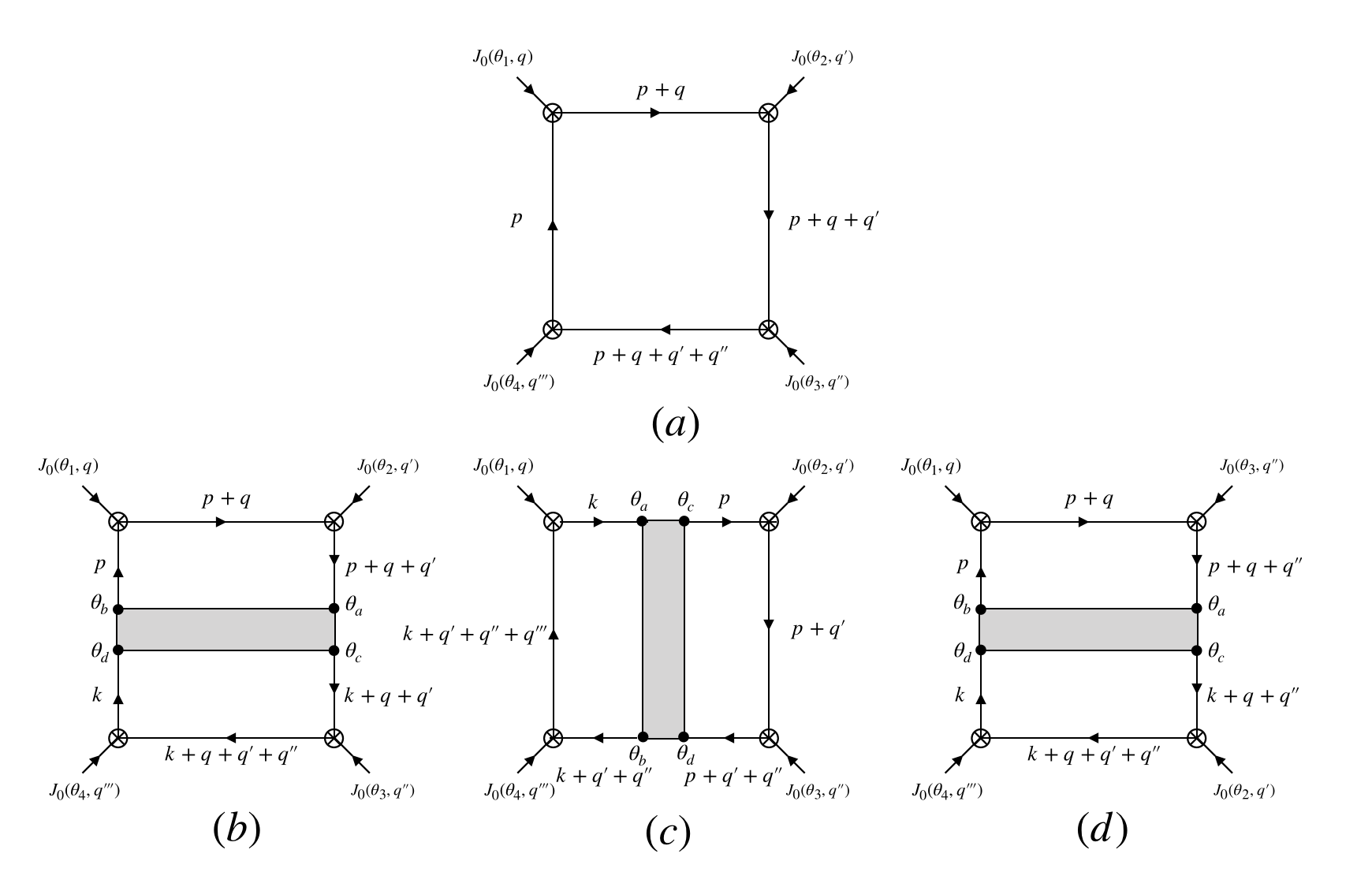
Figure 7: The contributing diagrams for the four point function of currents. The first diagram is diagram type (a). The grey blob in (b), (c) , (d) represents the all loop four point correlator. The remaining diagrams are obtained by permutations of the external operators.

For diagram one in 7, Note that the exact vertex (LABEL:J0vert) is a function of two internal grassmann variables. The propagators in fig (7) that emanate from/to the crossed vertices connect these internal Grassmann variables. So one has additional integration of 8 two-component internal Grassmann variables, these are not shown in the figure. In the exact three vertex (crossed), for the internal theta arguments, ${\mathcal{V}}_{3}(\theta_{1},\theta_{1}^{\prime},\theta_{1}^{\prime\prime},q,p)$ the primed theta is on the direction of the leaving momenta, and the double primed momenta are on the direction of the incoming momenta. The insertion momentum is the first momentum argument, and the incoming momentum is the second momentum argument. In fig (7) the diagram a is given by

$$V^{(A)}(q,q^{\prime},q^{\prime\prime},\theta_{1},\theta_{2},\theta_{3},\theta_{4})$$

$$=N\int\frac{d^{3}p}{(2\pi)^{3}}d^{2}\theta_{1}^{\prime}d^{2}\theta_{1}^{\prime\prime}d^{2}\theta_{2}^{\prime}d^{2}\theta_{1}^{\prime\prime}d^{2}\theta_{3}^{\prime}d^{2}\theta_{3}^{\prime\prime}d^{2}\theta_{4}^{\prime}d^{2}\theta_{4}^{\prime\prime}$$

$$\biggl{(}P(\theta_{1}^{\prime},\theta_{4}^{\prime\prime},p+q)P(\theta_{4}^{\prime},\theta_{3}^{\prime\prime},p-q^{\prime}-q^{\prime\prime})P(\theta_{3}^{\prime},\theta_{2}^{\prime\prime},p-q^{\prime})P(\theta_{2}^{\prime},\theta_{1}^{\prime\prime},p)$$

$${\mathcal{V}}_{3}(\theta_{1},\theta_{1}^{\prime},\theta_{1}^{\prime\prime},q,p){\mathcal{V}}_{3}(\theta_{2},\theta_{2}^{\prime},\theta_{2}^{\prime\prime},q^{\prime},p-q^{\prime}){\mathcal{V}}_{3}(\theta_{3},\theta_{3}^{\prime},\theta_{3}^{\prime\prime},q^{\prime\prime},p-q^{\prime}-q^{\prime\prime}){\mathcal{V}}_{3}(\theta_{4},\theta_{4}^{\prime},\theta_{4}^{\prime\prime},-q-q^{\prime}-q^{\prime\prime},p+q)\biggr{)}$$ (D.1)

There are a total of 6 additional diagrams due to permutations of the operators. and the interaction part is given by

$$V^{(B)}_{4}(q,q^{\prime},q^{\prime\prime},\theta_{1},\theta_{2},\theta_{3},\theta_{4})$$

$$=N^{2}\int\frac{d^{3}p}{(2\pi)^{3}}\frac{d^{3}k}{(2\pi)^{3}}d^{2}\theta_{a}d^{2}\theta_{b}d^{2}\theta_{c}d^{2}\theta_{d}d^{2}\theta_{1}^{\prime}d^{2}\theta_{1}^{\prime\prime}d^{2}\theta_{2}^{\prime}d^{2}\theta_{1}^{\prime\prime}d^{2}\theta_{3}^{\prime}d^{2}\theta_{3}^{\prime\prime}d^{2}\theta_{4}^{\prime}d^{2}\theta_{4}^{\prime\prime}$$

$$\biggl{(}P(\theta_{1}^{\prime},\theta_{4}^{\prime\prime},p+q)P(\theta_{4}^{\prime},\theta_{a},p-q^{\prime}-q^{\prime\prime})P(\theta_{c},\theta_{3}^{\prime\prime},k-q^{\prime}-q^{\prime\prime})P(\theta_{3}^{\prime},\theta_{2}^{\prime\prime},k-q^{\prime})P(\theta_{2}^{\prime},\theta_{d},k)P(\theta_{b},\theta_{1}^{\prime\prime},p)$$

$${\mathcal{V}}_{3}(\theta_{1},\theta_{1}^{\prime},\theta_{1}^{\prime\prime},q,p){\mathcal{V}}_{3}(\theta_{2},\theta_{2}^{\prime},\theta_{2}^{\prime\prime},q^{\prime},k-q^{\prime}){\mathcal{V}}_{3}(\theta_{3},\theta_{3}^{\prime},\theta_{3}^{\prime\prime},q^{\prime\prime},k-q^{\prime}-q^{\prime\prime}){\mathcal{V}}_{3}(\theta_{4},\theta_{4}^{\prime},\theta_{4}^{\prime\prime},-q-q^{\prime}-q^{\prime\prime},p+q)$$

$${\mathcal{V}}_{4}(\theta_{a},\theta_{b},\theta_{c},\theta_{d},p,-q^{\prime}-q^{\prime\prime},k)\biggr{)}$$ (D.2)

The bosonic and fermionic correlators for the diagram fig (7) are given by

$$\langle J_{0}^{b}(q)J_{0}^{b}(q^{\prime})J_{0}^{b}(q^{\prime\prime})J_{0}^{b}(-q-q^{\prime}-q^{\prime\prime})\rangle =V^{(1)}_{4}(q,q^{\prime},q^{\prime\prime},\theta_{1},\theta_{2},\theta_{3},\theta_{4})\biggl{|}_{\theta_{1}\to 0,\theta_{2}\to 0,\theta_{3}\to 0,\theta_{4}\to 0}$$

$$\langle J_{0}^{f}(q)J_{0}^{f}(q^{\prime})J_{0}^{f}(q^{\prime\prime})J_{0}^{f}(-q-q^{\prime}-q^{\prime\prime})\rangle =\prod_{i=1}^{4}\frac{\partial}{\partial\theta_{\alpha i}}\frac{\partial}{\partial\theta^{\alpha}_{i}}V^{(1)}_{4}(q,q^{\prime},q^{\prime\prime},\theta_{1},\theta_{2},\theta_{3},\theta_{4})$$ (D.3)

Although we were able to successfully perform the integrals for the components $p_{3},\theta_{p}$ and $k_{3},\theta_{k}$ in the expression for $V^{(B)}_{4}$ given by eq.(D.2) $k_{s}$ and $p_{s}$ integrals out be intractable analytically. Due to this difficulty we were not able to obtain a closed form expression for the four point function of the scalar operators$J_{0}^{b}$ and $J_{0}^{f}$ in eq.(D.3).

Appendix E AdS Contact diagrams

E.1 Closed-form

$$\bar{D}_{1111}(z,\bar{z})=\frac{1}{z-\bar{z}}[\ln(z\bar{z})\ln(\frac{1-z}{1-\bar{z}})+2\text{Li}_{2}(z)-2\text{Li}_{2}(\bar{z})]$$

$$\bar{D}_{2222}(z,\bar{z})=\frac{12uv}{(z-\bar{z})^{5}}+\frac{1+u+v}{(z-\bar{z})^{3}}[\ln(z\bar{z})\ln(\frac{1-z}{1-\bar{z}})+2\text{Li}_{2}(z)-2\text{Li}_{2}(\bar{z})]$$

$$+\frac{6}{(z-\bar{z})^{4}}\bigg{(}(1+u-v)v\ln v+(1+v-u)u\ln u\bigg{)}+\frac{2}{(z-\bar{z})^{2}}(\ln uv+1)$$

$$\bar{D}_{3333}(u,v)=$$

$$\bigg{(}\frac{1680u^{2}v^{2}}{(z-\bar{z})^{9}}+\bigg{(}\frac{240uv}{(z-\bar{z})^{7}}+\frac{24}{(z-\bar{z})^{5}}\bigg{)}(1+u+v)+\frac{4}{(z-\bar{z})^{3}}\bigg{)}[\ln(z\bar{z})\ln(\frac{1-z}{1-\bar{z}})+2\text{Li}_{2}(z)-2\text{Li}_{2}(\bar{z})]$$

$$+\bigg{(}\bigg{(}\frac{840u}{(z-\bar{z})^{8}}+\frac{100}{(z-\bar{z})^{6}}\bigg{)}v^{2}(1+u-v)+\frac{480uv}{(z-\bar{z})^{6}}+\frac{12(1+u)+76v}{(z-\bar{z})^{4}})\bigg{)}\ln v+u\leftrightarrow v$$

$$+\frac{260uv}{(z-\bar{z})^{6}}+\frac{26}{(z-\bar{z})^{4}}(1+u+v)$$ (E.1)

$$\bar{D}(u,v)_{3322}=-\partial_{u}\bar{D}_{2222}(u,v)$$

$$\bar{D}(u,v)_{4433}=-\partial_{u}\bar{D}_{3333}(u,v)$$ (E.2)

E.2 Decomposition in terms of conformal blocks

The contact diagrams may be written as an expansion in conformal blocks [59]

$$D_{\Delta\Delta\Delta^{\prime}\Delta^{\prime}}(x_{i})=\sum_{m}a^{\Delta\Delta}_{m}\alpha^{\Delta^{\prime}\Delta^{\prime}}_{m}\mathcal{W}_{\Delta_{m},0}(x_{i})+\sum_{n}a^{\Delta\Delta}_{n}\alpha^{\Delta^{\prime}\Delta^{\prime}}_{n}\mathcal{W}_{\Delta_{n},0}(x_{i})$$ (E.3)

$$D_{\Delta\Delta\Delta\Delta}(x_{i})=\sum_{n}2a^{\Delta\Delta}_{n}(\sum_{m\neq n}\frac{a^{\Delta\Delta}_{m}}{m^{2}_{n}-m^{2}_{m}})\mathcal{W}_{\Delta_{n},0}(x_{i})+\sum_{n}(a^{\Delta\Delta}_{n})^{2}\frac{\partial}{\partial m^{2}_{n}}\mathcal{W}_{\Delta_{n},0}(x_{i})$$ (E.4)

where $\mathcal{W}_{\Delta,0}=\beta_{\Delta 34}\beta_{\Delta 12}W_{\Delta,0}$. For $\Delta_{i}=\Delta$

$$D_{\Delta\Delta\Delta\Delta}(x_{i}) =\sum_{n}2a^{\Delta\Delta}_{n}\eta^{\Delta\Delta}_{n}\mathcal{W}_{\Delta_{n},0}(x_{i})+\sum_{n}(a^{\Delta\Delta}_{n})^{2}\frac{\partial}{\partial m^{2}_{n}}\mathcal{W}_{\Delta_{n},0}(x_{i})$$ (E.5)

$$=\sum_{n}[(2a^{\Delta\Delta}_{n}\eta^{\Delta\Delta}_{n}+(a^{\Delta\Delta}_{n})^{2})\beta^{2}_{\Delta_{n}\Delta\Delta}+\frac{\partial}{\partial m^{2}_{n}}\beta^{2}_{\Delta_{n}\Delta\Delta}]W_{\Delta_{n},0}(x_{i})$$

$$+\sum_{n}(a^{\Delta\Delta}_{n})^{2}\beta^{2}_{\Delta_{n}\Delta\Delta}\frac{\partial}{\partial m^{2}_{n}}W_{\Delta_{n},0}(x_{i})$$ (E.6)

with

$$\eta^{\Delta\Delta}_{n}=\sum_{m\neq n}\frac{a^{\Delta\Delta}_{m}}{m^{2}_{n}-m^{2}_{m}}$$ (E.7)

$$\beta_{\Delta 34}\equiv{\Gamma\left({\Delta+\Delta_{34}\over 2}\right)\Gamma\left({\Delta-\Delta_{34}\over 2}\right)\over 2\Gamma(\Delta)}$$ (E.8)

$$m_{\Delta_{k}}^{2}=\Delta_{k}(\Delta_{k}-d)$$

$$a^{12}_{m}=\frac{(-1)^{m}}{\beta_{\Delta_{m}12}m!}\frac{(\Delta_{1})_{m}(\Delta_{2})_{m}}{(\Delta_{1}+\Delta_{2}+m-d/2)_{m}}$$ (E.9)

with the anomalous dimension being proportional to the coefficient of the third term which involves derivative of the conformal block. Writing the above interms of the $\bar{D}$ functions

$$\bar{D}_{\Delta\Delta\Delta\Delta}(u,v) =\frac{1}{u^{\Delta}}[\sum_{n}[(2a^{\Delta\Delta}_{n}\eta^{\Delta\Delta}_{n})\beta^{2}_{\Delta_{n}\Delta\Delta}+(a^{\Delta\Delta}_{n})^{2}\frac{\partial}{\partial m^{2}_{n}}\beta^{2}_{\Delta_{n}\Delta\Delta}]G_{\Delta_{n},0}(u,v)$$

$$+\sum_{n}(a^{\Delta\Delta}_{n})^{2}\beta^{2}_{\Delta_{n}\Delta\Delta}\frac{\partial}{\partial m^{2}_{n}}G_{\Delta_{n},0}(u,v)]$$ (E.10)

We will re-label

$$P^{(\Delta)}_{1}(n,0)=(2a^{\Delta\Delta}_{n}\eta^{\Delta\Delta}_{n}+(a^{\Delta\Delta}_{n})^{2})\beta^{2}_{\Delta_{n}\Delta\Delta}+\frac{\partial}{\partial m^{2}_{n}}\beta^{2}_{\Delta_{n}\Delta\Delta}$$

$$P^{(\Delta)}_{0}(n,0)\gamma^{(\Delta)}_{1}(n,0)=2(a^{\Delta\Delta}_{n})^{2}\beta^{2}_{\Delta_{n}\Delta\Delta}$$ (E.11)

so that

$$\bar{D}_{\Delta\Delta\Delta\Delta}(u,v) =\frac{2\Gamma(\Delta)^{4}}{\Gamma(2\Delta-d/2)}\frac{1}{u^{\Delta}}\sum_{n}[P^{(\Delta)}_{1}(n,0)G_{\Delta_{n},0}(u,v)$$

$$+\frac{1}{2}P^{(\Delta)}_{0}(n,0)\gamma^{(\Delta)}_{1}(n,0)\frac{\partial}{\partial m^{2}_{n}}G_{\Delta_{n},0}(u,v)]$$ (E.12)

satisfying [60]

$$P^{(\Delta)}_{1}(n,0)=\frac{1}{2}\partial_{n}(P^{(\Delta)}_{0}(n,0)\gamma^{(\Delta)}_{1}(n,0))$$ (E.13)

Similarly, for (141)

$$\bar{D}_{\Delta+1\Delta+1\Delta\Delta}(u,v)= \frac{2\Gamma(\Delta)^{2}\Gamma(\Delta+1)^{2}}{\Gamma(2\Delta+1-d/2)}\frac{1}{u^{\Delta}}$$

$$[\sum_{m}\bar{P}^{(\Delta)}_{1}(n,0)G_{\Delta_{m},0}(u,v)+\frac{1}{2}\bar{P}^{(\Delta)}_{0}(n,0)\bar{\gamma}^{(\Delta)}_{1}(n,0)\frac{\partial}{\partial m^{2}_{n}}G_{\Delta_{n},0}(u,v)]$$

$$+\beta^{2}_{2\Delta}a^{\Delta\Delta}_{0}\eta^{\Delta+1\Delta+1}_{0}G_{2\Delta,0}(u,v)$$ (E.14)

$$\bar{P}^{(\Delta)}_{1}(n,0)=(a^{\Delta+1\Delta+1}_{n}\eta^{\Delta\Delta}_{n}+a^{\Delta\Delta}_{n}\eta^{\Delta+1\Delta+1}_{n})\beta^{2}_{\Delta_{n}\Delta\Delta}+a^{\Delta\Delta}_{n}a^{\Delta+1\Delta+1}_{n}\frac{\partial}{\partial m^{2}_{n}}\beta^{2}_{\Delta_{n}\Delta\Delta}$$

$$\bar{P}^{(\Delta)}_{0}(n,0)\bar{\gamma}^{(\Delta)}_{1}(n,0)=2a^{\Delta\Delta}_{n}a^{\Delta+1\Delta+1}_{n}\beta^{2}_{\Delta_{n}\Delta\Delta}$$ (E.15)

E.2.1 Examples

$$\bar{D}_{1111}(u,v)=\frac{2}{\pi^{1/2}u}\sum_{n}[P^{(1)}_{1}(n,0)G_{2+2n,0}(u,v)+\frac{1}{2}P^{(1)}_{0}(n,0)\gamma^{(1)}_{1}(n,0)\frac{\partial_{n}G_{2+2n,0}(u,v)}{8n+2}]$$

$$\bar{D}_{2222}(u,v)=\frac{8}{3\pi^{1/2}u^{2}}\sum_{n}[P^{(2)}_{1}(n,0)G_{4+2n,0}(u,v)+\frac{1}{2}P^{(2)}_{0}(n,0)\gamma^{(2)}_{1}(n,0)\frac{\partial_{n}G_{4+2n,0}(u,v)}{8n+10}]$$

$$\bar{D}_{3333}(u,v)=\frac{256}{105\pi^{1/2}u^{3}}\sum_{n}[P^{(3)}_{1}(n,0)G_{6+2n,0}(u,v)+\frac{1}{2}P^{(3)}_{0}(n,0)\gamma^{(3)}_{1}(n,0)\frac{\partial_{n}G_{6+2n,0}(u,v)}{8n+18}]$$ (E.16)

$$\bar{D}_{3322}(u,v)=\frac{64}{15\pi^{1/2}u^{3}}[\sum_{m}\bar{P}^{(3)}_{1}(m,0)G_{6+2m,0}(u,v)+\frac{1}{2}\bar{P}^{(3)}_{0}(m,0)\bar{\gamma}^{(3)}_{1}(m,0)\frac{\partial}{\partial m^{2}_{n}}G_{6+2m,0}(u,v)$$

$$+\beta^{2}_{4}a^{22}_{0}\eta^{33}_{0}G_{4,0}(u,v)]$$

$$\bar{D}_{4433}(u,v)=\frac{1024}{105\sqrt{\pi}u^{4}}[\sum_{m}\bar{P}^{(4)}_{1}(m,0)G_{8+2m,0}(u,v)+\frac{1}{2}\bar{P}^{(4)}_{0}(m,0)\bar{\gamma}^{(4)}_{1}(m,0)\frac{\partial}{\partial m^{2}_{n}}G_{8+2m,0}(u,v)$$

$$+\beta^{2}_{6}a^{33}_{0}\eta^{44}_{0}G_{6,0}(u,v)]$$ (E.17)

Contact terms for bosonic correlator

$$G^{AdS}_{\phi^{4}}=\bar{D}_{1111}(u,v)$$

$$G^{AdS}_{(\partial\phi)^{4}}=(1+u+v)\bar{D}_{2222}(u,v)$$

$$G^{AdS}_{\phi^{2}(\partial^{3}\phi)^{2}}=2(u^{2}\bar{D}_{3322}(u,v)+v^{2}\bar{D}_{3322}(v,u)+\frac{1}{v^{3}}\bar{D}_{3322}(1/v,u/v))$$ (E.18)

Contact terms for fermionic correlator

$$G^{AdS}_{\phi^{4}}=\bar{D}_{2222}(u,v)$$

$$G^{AdS}_{(\partial\phi)^{4}}=(1+u+v)\bar{D}_{3333}(u,v)$$

$$G^{AdS}_{\phi^{2}(\partial^{3}\phi)^{2}}=2(u^{2}\bar{D}_{4433}(u,v)+v^{2}\bar{D}_{4433}(v,u)+\frac{1}{v^{3}}\bar{D}_{4433}(1/v,u/v))$$ (E.19)

Appendix F Computing the coefficients

F.1 Bosonic case

We have derived similar relations for $\Delta\geq 4$ i.e. $n\geq 1$

$$[\tilde{C}^{2(BBB)}_{0,susy}]_{[O,O]_{n,0}} =\frac{1+\tilde{\lambda}^{4}}{\tilde{N}(1+\tilde{\lambda}^{2})^{2}}[\tilde{C}^{2}_{0,fb}]_{[O,O]_{n,0}}+c_{1}[\frac{2}{\pi^{1/2}}P^{(1)}_{1}(n,0)]+c_{2}[\frac{8}{3\pi^{1/2}}P^{(2)}_{1}(n-1,0)]$$

$$+c_{3}\frac{64}{15\pi^{1/2}}[\bar{P}^{(3)}_{1}(n-2,0)\Theta(n-1)+\beta^{2}_{4}a^{22}_{0}\eta^{33}_{0}\delta_{n-1,0}]$$ (F.1)

Let us take two arbitrary values of $n$ to solve for $c_{2}$ and $c_{3}$. Let them be $i,j$. So, the solution is, therefore,

$$c_{2}=\frac{E[j](A[i]+B[i]-C[i])-E[i](A[j]+B[j]-C[j])}{D[j]E[i]-D[i]E[j]}$$ (F.2)

$$c_{3}=\frac{D[j](A[i]+B[i]-C[i])-D[i](A[j]+B[j]-C[j])}{D[j]E[i]-D[i]E[j]}$$ (F.3)

where

$$A[n]=\frac{1+\tilde{\lambda}^{4}}{\tilde{N}(1+\tilde{\lambda}^{2})^{2}}[\tilde{C}^{2}_{0,fb}]_{[O,O]_{n,0}}$$

$$B[n]=c_{1}[\frac{2}{\pi^{1/2}}P^{(1)}_{1}(n,0)]$$

$$C[n]=[\tilde{C}^{2(BBB)}_{0,susy}]_{[O,O]_{n,0}}$$

$$D[n]=\frac{8}{3\pi^{1/2}}P^{(2)}_{1}(n-1,0)$$

$$E[n]=\frac{64}{15\pi^{1/2}}[\bar{P}^{(3)}_{1}(n-2,0)\Theta(n-1)+\beta^{2}_{4}a^{22}_{0}\eta^{33}_{0}\delta_{n-1,0}]$$ (F.4)

When $i=1,j=2$, we get

$$[\tilde{C}^{2(BBB)}_{0,susy}]_{[O,O]_{1,0}}=\frac{1+\tilde{\lambda}^{4}}{\tilde{N}(1+\tilde{\lambda}^{2})^{2}}[\tilde{C}^{2}_{0,fb}]_{[O,O]_{1,0}}+c_{1}[-0.0113728]+c_{2}[1.14329]+c_{3}[0.0891028]$$

$$[\tilde{C}^{2(BBB)}_{0,susy}]_{[O,O]_{2,0}}=\frac{1+\tilde{\lambda}^{4}}{\tilde{N}(1+\tilde{\lambda}^{2})^{2}}[\tilde{C}^{2}_{0,fb}]_{[O,O]_{2,0}}+c_{1}[5.78456*10^{-}6]+c_{2}[0.0151638]+c_{3}[9.58344]$$ (F.5)

so that

$$c_{2}=-0.874774~{}\frac{1+\tilde{\lambda}^{4}}{\tilde{N}(1+\tilde{\lambda}^{2})^{2}}[\tilde{C}^{2}_{0,fb}]_{[O,O]_{1,0}}+0.00793315~{}\frac{1+\tilde{\lambda}^{4}}{\tilde{N}(1+\tilde{\lambda}^{2})^{2}}[\tilde{C}^{2}_{0,fb}]_{[O,O]_{2,0}}$$

$$+0.874774[\tilde{C}^{2(BBB)}_{0,susy}]_{[O,O]_{1,0}}-0.00793315~{}[\tilde{C}^{2(BBB)}_{0,susy}]_{[O,O]_{2,0}}+0.00994867c_{1}$$ (F.6)

$$c_{3}=0.00138415~{}\frac{1+\tilde{\lambda}^{4}}{\tilde{N}(1+\tilde{\lambda}^{2})^{2}}[\tilde{C}^{2}_{0,fb}]_{[O,O]_{1,0}}-0.104359\frac{1+\tilde{\lambda}^{4}}{\tilde{N}(1+\tilde{\lambda}^{2})^{2}}[\tilde{C}^{2}_{0,fb}]_{[O,O]_{2,0}}$$

$$-0.00138415[\tilde{C}^{2(BBB)}_{0,susy}]_{[O,O]_{1,0}}+0.104359~{}[\tilde{C}^{2(BBB)}_{0,susy}]_{[O,O]_{2,0}}-0.0000163453~{}c_{1}$$ (F.7)

F.2 Fermionic case

We compute the OPE coefficient relations for scalar double-trace operators with $\Delta\geq 4$ using the methodology of the previous subsection.

$$[\tilde{C}^{2(FFF)}_{0,susy}]_{[O,O]_{n,0}} =\frac{1+\tilde{\lambda}^{4}}{\tilde{N}(1+\tilde{\lambda}^{2})^{2}}[\tilde{C}^{2}_{0,ff}]_{[O,O]_{n,0}}+\bar{c}_{1}[\frac{8}{3\pi^{1/2}}P^{(2)}_{1}(n,0)]+\bar{c}_{2}[\frac{256}{105\pi^{1/2}}\Theta(n)P^{(3)}_{1}(n-1,0)]$$

$$+\bar{c}_{3}\frac{1024}{105\sqrt{\pi}}[\bar{P}^{(4)}_{1}(n-2,0)\Theta(n-1)+\beta^{2}_{6}a^{33}_{0}\eta^{44}_{0}\delta_{n-1,0}]$$ (F.8)

References

- [1] S. Giombi, S. Minwalla, S. Prakash, S. P. Trivedi, S. R. Wadia, et al., Chern-Simons Theory with Vector Fermion Matter, Eur.Phys.J. C72 (2012) 2112, [arXiv:1110.4386].
- [2] O. Aharony, G. Gur-Ari, and R. Yacoby, d=3 Bosonic Vector Models Coupled to Chern-Simons Gauge Theories, JHEP 1203 (2012) 037, [arXiv:1110.4382].
- [3] J. Maldacena and A. Zhiboedov, Constraining Conformal Field Theories with A Higher Spin Symmetry, J.Phys. A46 (2013) 214011, [arXiv:1112.1016].
- [4] J. Maldacena and A. Zhiboedov, Constraining conformal field theories with a slightly broken higher spin symmetry, Class.Quant.Grav. 30 (2013) 104003, [arXiv:1204.3882].
- [5] O. Aharony, G. Gur-Ari, and R. Yacoby, Correlation Functions of Large N Chern-Simons-Matter Theories and Bosonization in Three Dimensions, JHEP 1212 (2012) 028, [arXiv:1207.4593].
- [6] S. Giombi, V. Gurucharan, V. Kirilin, S. Prakash, and E. Skvortsov, On the Higher-Spin Spectrum in Large N Chern-Simons Vector Models, JHEP 01 (2017) 058, [arXiv:1610.0847].
- [7] M. A. Vasiliev, Consistent equation for interacting gauge fields of all spins in (3+1)-dimensions, Phys. Lett. B243 (1990) 378–382.
- [8] M. A. Vasiliev, Higher spin gauge theories: Star product and AdS space, hep-th/9910096.
- [9] I. R. Klebanov and A. M. Polyakov, AdS dual of the critical O(N) vector model, Phys. Lett. B550 (2002) 213–219, [hep-th/0210114].
- [10] E. Sezgin and P. Sundell, Massless higher spins and holography, Nucl. Phys. B644 (2002) 303–370, [hep-th/0205131]. [Erratum: Nucl. Phys.B660,403(2003)].
- [11] S. Giombi and X. Yin, Higher Spin Gauge Theory and Holography: The Three-Point Functions, JHEP 09 (2010) 115, [arXiv:0912.3462].
- [12] S. Giombi and X. Yin, Higher Spins in AdS and Twistorial Holography, JHEP 04 (2011) 086, [arXiv:1004.3736].
- [13] O. Aharony, S. Giombi, G. Gur-Ari, J. Maldacena, and R. Yacoby, The Thermal Free Energy in Large N Chern-Simons-Matter Theories, JHEP 1303 (2013) 121, [arXiv:1211.4843].
- [14] S. Yokoyama, Chern-Simons-Fermion Vector Model with Chemical Potential, JHEP 1301 (2013) 052, [arXiv:1210.4109].
- [15] S. Jain, S. P. Trivedi, S. R. Wadia, and S. Yokoyama, Supersymmetric Chern-Simons Theories with Vector Matter, JHEP 1210 (2012) 194, [arXiv:1207.4750].
- [16] S. Yokoyama, A Note on Large N Thermal Free Energy in Supersymmetric Chern-Simons Vector Models, JHEP 1401 (2014) 148, [arXiv:1310.0902].
- [17] T. Takimi, Duality and higher temperature phases of large N Chern-Simons matter theories on x , JHEP 1307 (2013) 177, [arXiv:1304.3725].
- [18] S. Jain, S. Minwalla, T. Sharma, T. Takimi, S. R. Wadia, et al., Phases of large vector Chern-Simons theories on , JHEP 1309 (2013) 009, [arXiv:1301.6169].
- [19] S. Minwalla and S. Yokoyama, Chern Simons Bosonization along RG Flows, JHEP 02 (2016) 103, [arXiv:1507.0454].
- [20] G. Gur-Ari and R. Yacoby, Three Dimensional Bosonization From Supersymmetry, arXiv:1507.0437.
- [21] S. Choudhury, A. Dey, I. Halder, S. Jain, L. Janagal, S. Minwalla, and N. Prabhakar, Bose-Fermi Chern-Simons Dualities in the Higgsed Phase, JHEP 11 (2018) 177, [arXiv:1804.0863].
- [22] A. Dey, I. Halder, S. Jain, L. Janagal, S. Minwalla, and N. Prabhakar, Duality and an exact Landau-Ginzburg potential for quasi-bosonic Chern-Simons-Matter theories, JHEP 11 (2018) 020, [arXiv:1808.0441].
- [23] A. Dey, I. Halder, S. Jain, S. Minwalla, and N. Prabhakar, The large phase diagram of Chern-Simons theory with one fundamental chiral multiplet, arXiv:1904.0728.
- [24] Y. Dandekar, M. Mandlik, and S. Minwalla, Poles in the -Matrix of Relativistic Chern-Simons Matter theories from Quantum Mechanics, JHEP 1504 (2015) 102, [arXiv:1407.1322].
- [25] S. Jain, M. Mandlik, S. Minwalla, T. Takimi, S. R. Wadia, et al., Unitarity, Crossing Symmetry and Duality of the S-matrix in large N Chern-Simons theories with fundamental matter, JHEP 1504 (2015) 129, [arXiv:1404.6373].
- [26] K. Inbasekar, S. Jain, S. Mazumdar, S. Minwalla, V. Umesh, and S. Yokoyama, Unitarity, Crossing Symmetry and Duality in the scattering of Susy Matter Chern-Simons theories, arXiv:1505.0657.
- [27] S. Yokoyama, Scattering Amplitude and Bosonization Duality in General Chern-Simons Vector Models, JHEP 09 (2016) 105, [arXiv:1604.0189].
- [28] K. Inbasekar, S. Jain, P. Nayak, and V. Umesh, All tree level scattering amplitudes in Chern-Simons theories with fundamental matter, Phys. Rev. Lett. 121 (2018), no. 16 161601, [arXiv:1710.0422].
- [29] K. Inbasekar, S. Jain, S. Majumdar, P. Nayak, T. Neogi, T. Sharma, R. Sinha, and V. Umesh, Dual Superconformal Symmetry of Chern-Simons theory with Fundamental Matter and Non-Renormalization at Large , arXiv:1711.0267.
- [30] G. Gur-Ari and R. Yacoby, Correlators of Large N Fermionic Chern-Simons Vector Models, JHEP 1302 (2013) 150, [arXiv:1211.1866].
- [31] M. Geracie, M. Goykhman, and D. T. Son, Dense Chern-Simons Matter with Fermions at Large N, JHEP 04 (2016) 103, [arXiv:1511.0477].
- [32] G. Gur-Ari, S. A. Hartnoll, and R. Mahajan, Transport in Chern-Simons-Matter Theories, JHEP 07 (2016) 090, [arXiv:1605.0112].
- [33] R. Yacoby, Scalar Correlators in Bosonic Chern-Simons Vector Models, arXiv:1805.1162.
- [34] F. Benini, C. Closset, and S. Cremonesi, Comments on 3d Seiberg-like dualities, JHEP 1110 (2011) 075, [arXiv:1108.5373].
- [35] J. Park and K.-J. Park, Seiberg-like Dualities for 3d N=2 Theories with SU(N) gauge group, JHEP 10 (2013) 198, [arXiv:1305.6280].
- [36] O. Aharony, S. S. Razamat, N. Seiberg, and B. Willett, 3d dualities from 4d dualities, JHEP 07 (2013) 149, [arXiv:1305.3924].
- [37] A. Giveon and D. Kutasov, Seiberg Duality in Chern-Simons Theory, Nucl.Phys. B812 (2009) 1–11, [arXiv:0808.0360].
- [38] S. Jain, S. Minwalla, and S. Yokoyama, Chern Simons duality with a fundamental boson and fermion, JHEP 1311 (2013) 037, [arXiv:1305.7235].
- [39] O. Aharony, S. Jain, and S. Minwalla, Flows, Fixed Points and Duality in Chern-Simons-matter theories, JHEP 12 (2018) 058, [arXiv:1808.0331].
- [40] D. Radicevic, Disorder Operators in Chern-Simons-Fermion Theories, JHEP 03 (2016) 131, [arXiv:1511.0190].
- [41] O. Aharony, Baryons, monopoles and dualities in Chern-Simons-matter theories, JHEP 02 (2016) 093, [arXiv:1512.0016].
- [42] N. Seiberg, T. Senthil, C. Wang, and E. Witten, A Duality Web in 2+1 Dimensions and Condensed Matter Physics, Annals Phys. 374 (2016) 395–433, [arXiv:1606.0198].
- [43] A. Karch and D. Tong, Particle-Vortex Duality from 3d Bosonization, Phys. Rev. X6 (2016), no. 3 031043, [arXiv:1606.0189].
- [44] P.-S. Hsin and N. Seiberg, Level/rank Duality and Chern-Simons-Matter Theories, JHEP 09 (2016) 095, [arXiv:1607.0745].
- [45] J. Gomis, Z. Komargodski, and N. Seiberg, Phases Of Adjoint QCD3 And Dualities, SciPost Phys. 5 (2018), no. 1 007, [arXiv:1710.0325].
- [46] C. Cordova, P.-S. Hsin, and N. Seiberg, Global Symmetries, Counterterms, and Duality in Chern-Simons Matter Theories with Orthogonal Gauge Groups, SciPost Phys. 4 (2018), no. 4 021, [arXiv:1711.1000].
- [47] C. Cordova, P.-S. Hsin, and N. Seiberg, Time-Reversal Symmetry, Anomalies, and Dualities in (2+1), SciPost Phys. 5 (2018), no. 1 006, [arXiv:1712.0863].
- [48] M. A. Metlitski, A. Vishwanath, and C. Xu, Duality and bosonization of -dimensional majorana fermions, Phys. Rev. B 95 (May, 2017) 205137.
- [49] C. Córdova, P.-S. Hsin, and K. Ohmori, Exceptional Chern-Simons-Matter Dualities, arXiv:1812.1170.
- [50] I. Halder and S. Minwalla, Matter Chern Simons Theories in a Background Magnetic Field, arXiv:1904.0788.
- [51] G. J. Turiaci and A. Zhiboedov, Veneziano Amplitude of Vasiliev Theory, JHEP 10 (2018) 034, [arXiv:1802.0439].
- [52] O. Aharony, L. F. Alday, A. Bissi, and R. Yacoby, The Analytic Bootstrap for Large Chern-Simons Vector Models, JHEP 08 (2018) 166, [arXiv:1805.0437].
- [53] S. Caron-Huot, Analyticity in Spin in Conformal Theories, JHEP 09 (2017) 078, [arXiv:1703.0027].
- [54] O. Aharony and A. Sharon, Large N Renormalization Group Flows in 3d Chern-Simons-Matter Theories, arXiv:1905.0714.
- [55] R. Dijkgraaf and E. Witten, Topological Gauge Theories and Group Cohomology, Commun. Math. Phys. 129 (1990) 393.
- [56] A. A. Nizami, T. Sharma, and V. Umesh, Superspace formulation and correlation functions of 3d superconformal field theories, JHEP 07 (2014) 022, [arXiv:1308.4778].
- [57] H. Isono, T. Noumi, and G. Shiu, Momentum Space Approach to Crossing Symmetric CFT Correlators, JHEP 07 (2018) 136, [arXiv:1805.1110].
- [58] F. A. Dolan and H. Osborn, Conformal four point functions and the operator product expansion, Nucl. Phys. B599 (2001) 459–496, [hep-th/0011040].
- [59] E. Hijano, P. Kraus, E. Perlmutter, and R. Snively, Witten Diagrams Revisited: the AdS Geometry of Conformal Blocks, JHEP 01 (2016) 146, [arXiv:1508.0050].
- [60] I. Heemskerk, J. Penedones, J. Polchinski, and J. Sully, Holography from Conformal Field Theory, JHEP 10 (2009) 079, [arXiv:0907.0151].