Single Image Super-Resolution via CNN Architectures and TV-TV Minimization

Abstract

Super-resolution (SR) is a technique that allows increasing the resolution of a given image. Having applications in many areas, from medical imaging to consumer electronics, several SR methods have been proposed. Currently, the best performing methods are based on convolutional neural networks (CNNs) and require extensive datasets for training. However, at test time, they fail to impose consistency between the super-resolved image and the given low-resolution image, a property that classic reconstruction-based algorithms naturally enforce in spite of having poorer performance. Motivated by this observation, we propose a new framework that joins both approaches and produces images with superior quality than any of the prior methods. Although our framework requires additional computation, our experiments on Set5, Set14, and BSD100 show that it systematically produces images with better peak signal to noise ratio (PSNR) and structural similarity (SSIM) than the current state-of-the-art CNN architectures for SR.

1 Introduction

Image sensing technology is fundamentally limited by the physics of the acquisition process and often produces images with resolution below expectation. Super-resolution (SR) techniques overcome this by taking as input a low-resolution (LR) image and by outputting a high-resolution (HR) version of it. This, however, requires filling in the missing entries of the image, for which there are many possibilities. Predicting these entries thus requires making assumptions about the images, and different techniques make different assumptions. Landmark techniques include polynomial interpolation methods, which assume that images are spatially smooth and well approximated by bilinear or bicubic functions [Keys(1981), Blu et al.(2004)Blu, Thevenaz, and Unser], reconstruction methods, which assume that images have sparse representations in certain domains that are fixed [Fattal(2007), Sen and Darabi(2009), Sun et al.(2008)Sun, Xu, and Shumand] or that can be learned from training data [Yang et al.(2010)Yang, Wright, Huang, and Ma, Zeyde et al.(2012)Zeyde, Elad, and Protter], and convolutional neural network (CNN) architectures [Dong et al.(2014)Dong, Loy, He, and Tang, Kim et al.(2016)Kim, Lee, and Lee, Ledig et al.(2017)Ledig, Theis, Huszár, Caballero, Cunningham, Acosta, Aitken, Tejani, Totz, Wang, and Shi], which assume that image patches share high-level features that can be learned by a CNN.

Indeed, the best performing SR methods are based on CNNs [Dong et al.(2014)Dong, Loy, He, and Tang, Kim et al.(2016)Kim, Lee, and Lee, Ledig et al.(2017)Ledig, Theis, Huszár, Caballero, Cunningham, Acosta, Aitken, Tejani, Totz, Wang, and Shi]. Although they produce outstanding results, CNNs have well-known shortcomings: they require extensive data and computational resources for training, they have limited theoretical guarantees and, when the training data is not representative, they may fail to generalize. Reconstruction methods, on the other hand, typically super-resolve images via optimization algorithms, which confers them more interpretability and equips them with theoretical guarantees. They use regularizers to directly encode prior knowledge about images, e.g., that they have relatively few edges, sparse representations in some domain, or many recurring patterns. Although this direct encoding of prior knowledge dispenses reconstruction-based methods from a training stage, they are outperformed by learning-based methods.

Our framework. We propose a framework that joins reconstruction and learning techniques. Our motivating observation is that the best learning techniques, namely CNN architectures, ignore important information at test time: they fail to guarantee that the given input image matches their output when downsampled. Reconstruction algorithms, on the other hand, impose this constraint naturally. Our main idea is then to integrate the HR output of a learning-based method into a reconstruction scheme, i.e., we use an image super-resolved by a learning-based method as side information in a reconstruction-based method. For the latter, we adopt a SR algorithm based on total variation (TV) minimization, a prior that encodes the fact that images have a small number of edges. This simple prior is enough to illustrate the benefits of our framework which, nevertheless, can be adapted to more complex priors.

Our framework introduces a simple post-processing step that requires some additional computation. However, as our experiments show, it systematically improves the outputs of several CNN architectures, producing images with better peak signal to noise ratio (PSNR) and structural similarity (SSIM) [Wang et al.(2004)Wang, Bovik, Sheikh, and Simoncelli].

2 Related Work

Single-image SR algorithms can be split into interpolation, reconstruction, and learning methods. We focus our overview on reconstruction and learning methods, as both outperform interpolation-based schemes.

2.1 Reconstruction-based SR

Reconstruction-based methods super-resolve images with an algorithm that solves an optimization problem usually containing two terms: one ensuring that the downsampled solution coincides with the input LR image and another encoding prior knowledge about images.

Statistical models. The work in [Fattal(2007)] models the gradient profile of an image as a Gauss-Markov random field and performs SR via maximum likelihood estimation with the constraint that downsampled solution coincides with the given LR image. In [Sun et al.(2008)Sun, Xu, and Shumand], images are super-resolved by ensuring that the gradient of the HR image is close to a gradient profile obtained from the LR image using a similar, but parametric model, while imposing again that the downsampled solution coincides with the given LR image.

Total variation methods. A different line of work directly encodes prior knowledge into the optimization problem. For instance, [Rudin et al.(1992)Rudin, Osher, and Fatemi] introduced the concept of TV to capture the number of edges in an image and observed that natural images have small TV. Since then, several algorithms have been proposed to super-resolve images by minimizing TV. For example, [Morse and Schwartzwald(2001)] addresses the problem by discretizing a differential equation that relates changes in the values of individual pixels to the curvature of level sets. More recently, with the development of nondifferentiable convex optimization methods, TV minimization has been addressed in the discrete setting by a wide range of algorithms [Chambolle(2004), Bioucas-Dias and Figueiredo(2007), Goldstein and Osher(2009), Becker et al.(2011)Becker, Bobin, and Candès, Li et al.(2013)Li, Yin, Jiang, and Zhang]. There are essentially two versions of discrete TV, according to the norm that is applied to the discretized gradient at each pixel: isotropic ($\ell_{2}$-norm) and anisotropic ($\ell_{1}$-norm); see, e.g., [Bioucas-Dias and Figueiredo(2007), Li et al.(2013)Li, Yin, Jiang, and Zhang]. Since both versions are convex, discrete TV minimization algorithms not only have small computational complexity (as matrix-vector operations can be performed via the FFT algorithm), but are also guaranteed to find a global minimizer.

Alternative regularizers. Natural images also have simple representations in other domains, and other regularizers have been used for SR. For example, [Sen and Darabi(2009)] uses the fact that images have sparse wavelet representations. The patches of natural images also tend to lie on a low-dimensional manifold [Lee et al.(2003)Lee, Pedersen, and Mumford], which has motivated nonlocal methods. These use as regularizers (nonconvex) functions that enforce many patches of an image to have similar features; see, e.g., [Peyré et al.(2008)Peyré, Bougleux, and Cohen, Protter et al.(2009)Protter, Elad, Takeda, and Milanfar]. Finally, different regularizers can be combined as in [Shi et al.(2015)Shi, Cheng, Wang, Yap, and Shen, Li et al.(2016)Li, Wu, Deng, and Liu].

2.2 Learning-based SR

Learning-based methods usually operate on patches and learn how to map a LR to a HR patch. They consist of a training stage, in which the map is learned, and a testing stage, in which the map is applied to the LR patches to obtain HR patches.

Coding and dictionary learning. Coding and dictionary learning algorithms super-resolve the patches of an image by linearly combining HR patches collected (or created) from other images during training. An early method is [Chang et al.(2004)Chang, Yueng, and Xiong], which adapts the locally linear embedding algorithm of [Roweis and Saul(2000)] for SR. Drawing from developments in sparse-based reconstruction, [Yang et al.(2010)Yang, Wright, Huang, and Ma] proposed using training images to learn two dictionaries, one for HR and another for LR patches, such that corresponding HR and LR patches have the same coefficients; see [Zeyde et al.(2012)Zeyde, Elad, and Protter] for a similar approach. While these schemes rely on other images to learn the LR-HR map, [Singh et al.(2014)Singh, Porikli, and Ahuja, Huang et al.(2015)Huang, Singh, and Ahuja] use self-similarity to learn the map without using other images.

Regression methods. Regression methods compute the LR-HR map using a set of basis functions whose coefficients are computed via regression. The key idea is to perform clustering on the training images, and use algorithms like kernel ridge regression (KRR) [Kim and Kwon(2010)], Gaussian process regression [He and Siu(2011)] and random forests [Schulter et al.(2015)Schulter, Leistner, and Bischof] to perform SR.

CNN-based. Currently, the best performing SR methods are based on CNNs. Taking inspiration in the dictionary learning algorithm in [Yang et al.(2010)Yang, Wright, Huang, and Ma], SRCNN [Dong et al.(2014)Dong, Loy, He, and Tang] was one of the first CNNs performing image SR. It consists of a patch extraction layer, a representation layer of the non-linear mappings, and a final layer that outputs the reconstructed image. As most neural network architectures, SRCNN requires an extensive training set, and has to be retrained for each different upscaling factor. To overcome the latter problem, DRCN [Kim et al.(2016)Kim, Lee, and Lee] uses a recursive convolutional layer that is repeatedly applied to obtain SR. Building on generative adversarial networks [Goodfellow et al.(2014)Goodfellow, Abadie, Mirza, Xu, Farley, Ozair, Courville, and Bengio], state-of-the-art SR results are obtained in [Ledig et al.(2017)Ledig, Theis, Huszár, Caballero, Cunningham, Acosta, Aitken, Tejani, Totz, Wang, and Shi]. It proposes two networks: SRGAN, which produces photo-realistic images with high perceptual quality, and SRResNet, which achieves the best PSNR and SSIM compared to all prior SR approaches. Although CNN-based methods achieve state-of-the-art SR results, they suffer from a major shortcoming that leaves room for improvement: in general, they fail to impose consistency between the HR and LR image in the testing stage. Such consistency, however, is always enforced by reconstruction-based (specifically, optimization-based) algorithms. This observation is the main motivation behind our framework, which we introduce next.

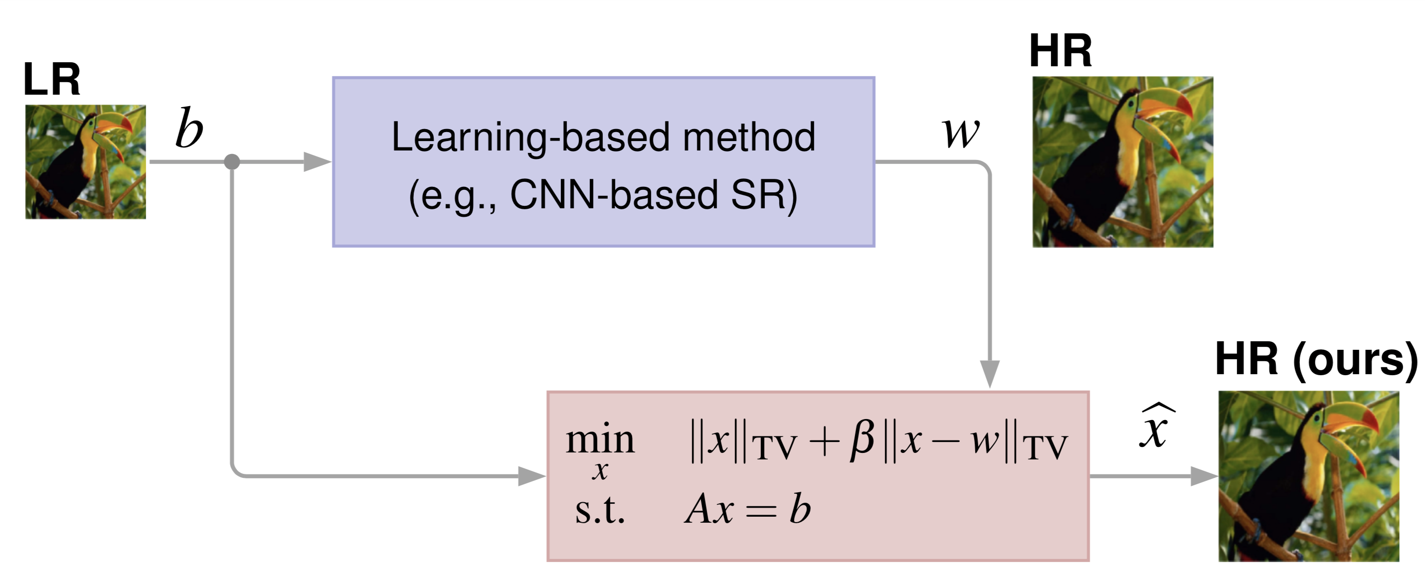
Figure 1: Our framework: a learning-based method super-resolves $b$ into $w$, and both images are then used to find the final estimate $\widehat{x}$ of a TV-TV minimization problem.

3 Our Framework

Given a low-resolution (LR) image, our goal is to build a high-resolution (HR) version of it. Before describing how we achieve this, we introduce our model and assumptions.

Model and assumptions. We denote by $X^{\star}\in\mathbb{R}^{M\times N}$ the HR image, and by $x^{\star}\mathrel{\mathop{\ordinarycolon}}=\text{vec}(X^{\star})\in\mathbb{R}^{n}$ its column-major vectorization, where $n\mathrel{\mathop{\ordinarycolon}}=M\cdot N$. Since these represent 2D quantities, we will always work either with grayscale images or with specific channels of a given representation of color images. We assume that $X^{\star}$ has a small number of edges. Namely, we assume $\|x^{\star}\|_{\text{TV}}\mathrel{\mathop{\ordinarycolon}}=\sum_{i=1}^{M}\sum_{j=1}^{N}|D_{ij}^{v}x^{\star}|+|D_{ij}^{h}x^{\star}|$ is small, where $D_{ij}^{v}$ (resp. $D_{ij}^{h}$) is a row-vector that extracts the vertical (resp. horizontal) difference at pixel $(i,j)$ of $X^{\star}$. Notice that this corresponds to the anisotropic TV-norm [Bioucas-Dias and Figueiredo(2007), Li et al.(2013)Li, Yin, Jiang, and Zhang], which can be written more succinctly as $\|x^{\star}\|_{\text{TV}}=\|Dx^{\star}\|_{1}$, where the rows of $D\in\mathbb{R}^{2n\times n}$ contain all the $D_{ij}^{v}$’s and $D_{ij}^{h}$’s. We assume periodic boundary conditions, so that matrix-vector products can be efficiently computed via the FFT algorithm.

The vectorization of the given LR image will be denoted by $b\in\mathbb{R}^{m}$, where $m<n$. We assume the LR and HR vectorizations are linearly related as $b=Ax^{\star}$, where $A\in\mathbb{R}^{m\times n}$ is a downsampling operator, i.e., $Ax^{\star}$ represents a downsampled version of $x^{\star}$, which can be obtained via filtering (e.g., bicubic or box) or even direct sampling. As bicubic filtering is a popular downsampling operator, and is the preferred method for generating training data for CNNs, we will assume that A implements such (linear) operator.

Proposed framework. Fig. 1 shows the main components of our framework. It builds on a base method which, because of their current state-of-the-art performance, will be a learning-based scheme. The LR image $b$ is fed into the base method, which super-resolves it into a HR image that we will denote by $w\in\mathbb{R}^{n}$. As mentioned in Section 2, learning-based schemes, namely the ones based on CNN architectures, fail to enforce consistency between the LR and HR images during testing. That is, in our notation, fail to guarantee $Ax^{\star}=b$. As shown in Fig. 1, we thus propose an additional stage, which processes both the given LR image $b$ and the HR image $w$ from the learning-based method to build our final estimate $\widehat{x}$ of $x^{\star}$. That stage solves a problem that we call TV-TV minimization.

TV-TV minimization. Inspired by the success of sparse reconstruction schemes that integrate prior information in the form of past, similar examples [Chen et al.(2008)Chen, Tang, and Leng, Weizman et al.(2016)Weizman, Eldar, and Ben-Bashat, Mota et al.(2017)Mota, Deligiannis, and Rodrigues], we propose to estimate $x^{\star}$ by solving an optimization problem whose objective balances the TV-norm of the optimization variable $x$ and the TV-norm of the difference between $x$ and $w$, while constraining $Ax=b$. That is, we obtain the final estimate $\widehat{x}\,$ by solving TV-TV minimization:

$$\begin{array}[t]{ll}\underset{x}{\text{minimize}}&\|x\|_{\text{TV}}+\beta\|x-w\|_{\text{TV}}\\ \text{subject to}&Ax=b\,,\end{array}$$ (1)

where $\beta\geq 0$ is a tradeoff parameter. Since the constraints of (1) are linear and the TV-norm is convex, problem (1) is convex. To our knowledge, the first instance of (1) appeared in [Chen et al.(2008)Chen, Tang, and Leng] in the context of dynamic CT imaging, where $w$ was a coarse estimation of the image to be reconstructed. The work in [Weizman et al.(2016)Weizman, Eldar, and Ben-Bashat] generalized that approach, in the context of MRI imaging, to the case where the TV-norms are weighted, and their weights are updated as in [Candès et al.(2008)Candès, Wakin, and Boyd]. There, $w$ represented a reference image, i.e., an image similar to the image to reconstruct.

Problem (1) enforces consistency between the LR image $b$ and the final estimate $\widehat{x}$ via the constraint $Ax=b$. Among the possible solutions of $Ax=b$, it seeks the one that has a small TV-norm and, at the same time, does not deviate much from $w$, in the sense that their discrete gradients are similar. While it is also possible to enforce pixel-level similarity, we found that imposing similarity of gradients produces the best results.

As mentioned in Section 2.1, it is possible to use alternative regularizers that capture other properties of natural images, or even combine several different regularizers. Indeed, the reason why we are proposing a “framework” and not just a “method” is because we allow both blocks in Fig. 1 to vary. Using TV-TV minimization (1), however, enables us to draw from the insights in [Mota et al.(2017)Mota, Deligiannis, and Rodrigues] for $\ell_{1}$-$\ell_{1}$ minimization.

Connections with $\ell_{1}$-$\ell_{1}$ minimization. Since $\|x\|_{\text{TV}}=\|Dx\|_{1}$, by introducing an additional variable $\mathbb{R}^{2n}\ni z=Dx$, we rewrite (1) as

$$\begin{array}[t]{ll}\underset{z,x}{\text{minimize}}&\|z\|_{1}+\beta\|z-\overline{w}\|_{1}\\ \text{subject to}&Ax=b\,,\,\,\,\,\,\,Dx=z\,,\end{array}$$ (2)

where we defined $\overline{w}\mathrel{\mathop{\ordinarycolon}}=Dw$. We denote the concatenation of the optimization variables as $\overline{x}\mathrel{\mathop{\ordinarycolon}}=(z,x)\in\mathbb{R}^{3n}$ and define $\overline{A}\mathrel{\mathop{\ordinarycolon}}=\begin{bmatrix}0_{m\times 2n}&A;&-I_{2n}&D\end{bmatrix}$, and $\overline{b}\mathrel{\mathop{\ordinarycolon}}=\begin{bmatrix}b&0_{2n}\end{bmatrix}^{\top}$, where $0_{a\times b}$ (resp. $0_{a}$) stands for the zero matrix (resp. vector) of dimensions $a\times b$ (resp. $a\times 1$), and $I_{2n}$ is the identity matrix in $\mathbb{R}^{2n}$. This enables us to further rewrite (2) as

$$\begin{array}[t]{ll}\underset{\overline{x}}{\text{minimize}}&\|P_{2n}\overline{x}\|_{1}+\beta\|P_{2n}\overline{x}-\overline{w}\|_{1}\\ \text{subject to}&\overline{A}\overline{x}=\overline{b}\,,\end{array}$$ (3)

where $P_{2n}\in\mathbb{R}^{2n\times 3n}$ contains the first $2n$ rows of the identity matrix in $\mathbb{R}^{3n}$, $I_{3n}$. That is, for a vector $v\in\mathbb{R}^{3n}$, $P_{2n}v$ extracts the first $2n$ components of $v$. The work in [Mota et al.(2017)Mota, Deligiannis, and Rodrigues] characterized the performance of the problem in (3) when $P_{2n}$ is the full identity matrix, rather than just part of it, a problem they called $\ell_{1}$-$\ell_{1}$ minimization. Assuming that $\overline{A}$ has Gaussian random entries, [Mota et al.(2017)Mota, Deligiannis, and Rodrigues] provided precise reconstruction guarantees for such a problem. In particular, they showed that $\beta=1$ yields the best performance in theory and in practice. Although these results were proved only for the case in which $\overline{A}$ is a Gaussian matrix, experiments in [Mota et al.(2016)Mota, Deligiannis, Sankaranarayanan, Cevher, and Rodrigues] suggest that they also hold for other types of matrices. This led us to select $\beta=1$ in all our experiments.

Solving (1). A disadvantage of our framework compared to learning-based methods, in particular CNN architectures, is that solving an optimization problem like (1) requires some computation. Yet, because the downsampling matrix $A$ and difference matrix $D$ are very structured, we can design algorithms that take advantage of fast matrix-vector multiplications. Specifically, given $u\in\mathbb{R}^{n}$ and $v\in\mathbb{R}^{m}$, $Au$ outputs a subvector of $u$, and $A^{\top}v$ outputs an $n$-dimensional vector whose entries are the entries of $v$ (at locations specified by $A$) or zeros. These operations require neither explicit construction of $A$, nor any floating-point operation (just memory access). Because we assume periodic boundary conditions, the matrix-vector products $Du$ and $D^{\top}v$, for $u\in\mathbb{R}^{n}$ and $v\in\mathbb{R}^{2n}$, can be efficiently computed using the FFT algorithm, which requires $O(n\log n)$ floating-point operations; see [Li et al.(2013)Li, Yin, Jiang, and Zhang].

To solve (1), we apply ADMM [Boyd et al.(2011)Boyd, Parikh, Chu, Peleato, and Eckstein], guaranteeing that its implementation uses only matrix-vector products as above. ADMM is applied directly to problem (2) with the splitting $f(z,x)=\|z\|_{1}+\beta\|z-w\|_{1}$ and $g(x,z)=\text{i}_{\{(z,x)\,\mathrel{\mathop{\ordinarycolon}}\,Ax=b,\,Dx=z\}}(z,x)$, where $\text{i}_{S}(u)$ is an indicator function, i.e., $\text{i}_{S}(u)=0$ if $u\in S$, and $\text{i}_{S}(u)=+\infty$ otherwise. Our focus was not on obtaining the most efficient implementation, but we point out possible improvements in Section 5.

4 Experiments

We tested our framework on the standard test sets Set5 [Bevilacqua et al.(2012)Bevilacqua, Roumy, Guillemot, and Morel], Set14 [Zeyde et al.(2012)Zeyde, Elad, and Protter], and BSD100 [Martin et al.(2001)Martin, Fowlkes, Tal, and Malik], each containing respectively 5, 14, and 100 images. For RGB images, we only super-resolved the luminance channel of the YCbCr color space, as in [Huang et al.(2015)Huang, Singh, and Ahuja, Dong et al.(2014)Dong, Loy, He, and Tang, Kim et al.(2016)Kim, Lee, and Lee, Ledig et al.(2017)Ledig, Theis, Huszár, Caballero, Cunningham, Acosta, Aitken, Tejani, Totz, Wang, and Shi]. All our experiments were run on the same machine with a 12 core 2.10 GHz Intel(R) Xeon(R) Silver 4110 CPU and two Nvidia GeForce RTX GPUs. The code used for all experiments is available online.

We used four state-of-the art learning schemes: KRR by Kim [Kim and Kwon(2010)], self-similarity [Huang et al.(2015)Huang, Singh, and Ahuja], pre-trained CNNs [Dong et al.(2014)Dong, Loy, He, and Tang, Kim et al.(2016)Kim, Lee, and Lee] and basic TV minimization, i.e., (1) with $\beta=0$, using TVAL3 [Li et al.(2013)Li, Yin, Jiang, and Zhang]. Of these methods, only [Li et al.(2013)Li, Yin, Jiang, and Zhang] operates on full images, just like our TV-TV minimization algorithm; all the remaining methods operate only on patches. The output images of SRCNN [Dong et al.(2014)Dong, Loy, He, and Tang], Kim [Kim and Kwon(2010)] and SelfExSR [Huang et al.(2015)Huang, Singh, and Ahuja] were obtained from the repository.

As our framework is tied to a given base method, whenever the latter changes, so does our method. For assessing performance, we used PSNR and SSIM [Wang et al.(2004)Wang, Bovik, Sheikh, and Simoncelli] computed on the luminance channel.

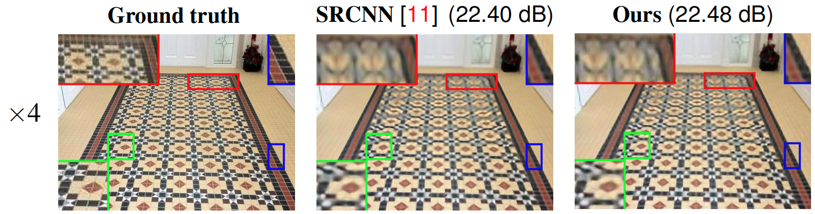
Figure 2: Performance of our method, using SRCNN [Dong et al.(2014)Dong, Loy, He, and Tang] as the base method, for an image not included in any of the training or test sets. The ground truth was downsampled by $4$ and then super-resolved with SRCNN and our method. PSRN values are shown in parenthesis.

4.1 Illustrating consistency between LR and HR images

To demonstrate how imposing consistency between the LR and HR images can improve SR performance, we conducted an experiment using an image that is not in any of the above datasets. The image, of dimensions 472 $\times$ 352, is shown in the left of Fig. 2 and was selected because of its structured patterns. We downsampled it via bicubic filtering by a factor of $4$, and then reconstructed it with the CNN architecture SRCNN [Dong et al.(2014)Dong, Loy, He, and Tang], and with our method using SRCNN as the base algorithm. Since SRCNN fails to enforce consistency between the LR and HR images during testing, its output (Fig. 2, center) blurs the tiles and removes some details. Our method, which uses the output of SRCNN (Fig. 2, center) and the $4\times$ downscaled version of the ground truth (Fig. 2), seems to reduce the blur artifacts, as manifested by an improvement in the PSNR. Such an improvement, however, comes with a computational cost: to super-resolve that image required SRCNN 2 seconds, and solving (1) required 151 seconds.

4.2 Experiments on Set4, Set5, and BSD100

Tab. 1 shows the results of our experiments for the testing datasets Set5, Set14, and BSD100. It displays the PSNR and SSIM values for $2\times$ and $4\times$ upscaling tasks, and these values represent averages over all the images in the corresponding dataset. Recall that higher PSNR and SSIM values reflect better performance. The table has 5 parts, one for each variation of the base method. For example, the first 3 rows refer to the results when the method in Kim [Kim and Kwon(2010)] is the base algorithm; in the next 3 rows, the base method is SRCNN [Dong et al.(2014)Dong, Loy, He, and Tang], and so on. The values for TVAL3 [Li et al.(2013)Li, Yin, Jiang, and Zhang] are repeated in all parts of the table, since its input is the same image in all the cases.

It can be observed that TVAL3, an algorithm for solving (1) with $\beta=0$, yields the worst performance. All the learning-based methods (4th column) systematically give results better than TVAL3. Our method (last column), in turn, uses the outputs of those algorithms and, by enforcing consistency between the LR and HR images, systematically improves their outputs: for example, the range of the gains in PSNR values was $0.006$-$0.177$ dB.

Fig. 3 shows the reconstructions of a particular image in Set14 for all the methods. The top-left box corresponds to the ground truth and TVAL3, which were the same in all the experiments. The remaining boxes show the results of a given learning-based method and the corresponding output using our framework. As in Section 4.1, it can be seen that the learning-based methods tend to produce images that lack details and they fail to impose consistency with the given LR image. Our method, in contrast, constraints the LR image to be consistent with the HR image which improves the image quality and slightly reduces the blurring effect. The execution times of SRCNN [Dong et al.(2014)Dong, Loy, He, and Tang] and DRCN [Kim et al.(2016)Kim, Lee, and Lee] to super-resolve the sample image in Fig. 3 are shown in Tab. 2. Although our method yields better PSNR/SSIM values, it requires significantly more computational time.

5 Conclusions

We proposed a framework for super-resolving images that leverages the good performance of learning-based methods, including CNN architectures, and the consistency enforced by reconstruction-based algorithms. The framework takes a base learning-method, and improves its output by solving a TV-TV minimization problem. Although the image model we used is quite simple, it suffices to illustrate the reconstruction gains in PSNR and SSIM that can be obtained. Our experimental results involving several state-of-the-art SR algorithms show that the proposed framework achieves some performance gains over those algorithms, however, at an additional computation cost.

Possible research directions include using regularizers that capture more realistic image assumptions and accelerating the algorithm for solving the TV-TV minimization algorithm e.g., using a C implementation, or a trained recurrent neural network as a solver [Gregor and LeCun(2010)].

Table 1: Average PSNR (SSIM) results using the reference methods.

Dataset		Scale		TVAL3 [Li et al.(2013)Li, Yin, Jiang, and Zhang]		Kim [Kim and Kwon(2010)]	Ours
Set5		$\times 2$		34.0315 (0.9354)		36.2465 (0.9516)	36.4499 (0.9537)
		$\times 4$		29.1708 (0.8349)		30.0730 (0.8553)	30.2289 (0.8593)
Set14		$\times 2$		31.0033 (0.8871)		32.1359 (0.9031)	32.3044 (0.9055)
		$\times 4$		26.6742 (0.7278)		27.1836 (0.7434)	27.2993 (0.7488)
BSD100		$\times 2$		30.1373 (0.8671)		31.1124 (0.8840)	31.2097 (0.8864)
		$\times 4$		26.3402 (0.6900)		26.7099 (0.7027)	26.7891 (0.7086)
Dataset		Scale		TVAL3 [Li et al.(2013)Li, Yin, Jiang, and Zhang]		SRCNN [Dong et al.(2014)Dong, Loy, He, and Tang]	Ours
Set5		$\times 2$		34.0315 (0.9354)		36.2772 (0.9509)	36.5288 (0.9536)
		$\times 4$		29.1708 (0.8349)		30.0765 (0.8525)	30.2669 (0.8590)
Set14		$\times 2$		31.0033 (0.8871)		31.9954 (0.9012)	32.2949 (0.9057)
		$\times 4$		26.6742 (0.7278)		27.1254 (0.7395)	27.3040 (0.7480)
BSD100		$\times 2$		30.1373 (0.8671)		31.1087 (0.8835)	31.2241 (0.8866)
		$\times 4$		26.3402 (0.6900)		26.7027 (0.7018)	26.7838 (0.7085)
Dataset		Scale		TVAL3 [Li et al.(2013)Li, Yin, Jiang, and Zhang]		SelfExSR [Huang et al.(2015)Huang, Singh, and Ahuja]	Ours
Set5		$\times 2$		34.0315 (0.9354)		36.5001 (0.9537)	36.5321 (0.9542)
		$\times 4$		29.1708 (0.8349)		30.3317 (0.8623)	30.3370 (0.8625)
Set14		$\times 2$		31.0033 (0.8871)		32.2272 (0.9036)	32.3951 (0.9059)
		$\times 4$		26.6742 (0.7278)		27.4014 (0.7518)	27.4730 ( 0.7536)
BSD100		$\times 2$		30.1373 (0.8671)		31.1833 (0.8855)	31.2056 (0.8862)
		$\times 4$		26.3402 (0.6900)		26.8459 (0.7108)	26.8482 (0.7108)
Dataset		Scale		TVAL3 [Li et al.(2013)Li, Yin, Jiang, and Zhang]		DRCN [Kim et al.(2016)Kim, Lee, and Lee]	Ours
Set5		$\times 2$		34.0315 (0.9354)		37.6279 (0.9588)	37.6712 (0.9591)
		$\times 4$		29.1708 (0.8349)		31.5344 (0.8854)	31.5701 (0.8858)
Set14		$\times 2$		31.0033 (0.8871)		33.0585 (0.9121)	33.1038 (0.9129)
		$\times 4$		26.6742 (0.7278)		28.0269 (0.7673)	28.0588 (0.7680)
BSD100		$\times 2$		30.1373 (0.8671)		31.8536 (0.8942)	31.8737 (0.8953)
		$\times 4$		26.3402 (0.6900)		27.2364 (0.7233)	27.2524 (0.7240)

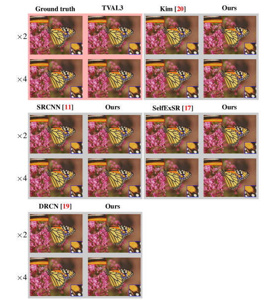
Figure 3: Reconstructions of the Monarch image (Set14) for all the methods in Tab. 1. Some details are highlighted (best viewed by zooming in on a computer screen).

Table 2: Execution times (in secs) for reconstructing the image in Fig. 3.

				Base: SRCNN [Dong et al.(2014)Dong, Loy, He, and Tang]				Base: DRCN [Kim et al.(2016)Kim, Lee, and Lee]
Scale		TVAL3 [Li et al.(2013)Li, Yin, Jiang, and Zhang]		SRCNN		Ours		DRCN		Ours
$\times 2$		3.34		9.31		307.84		156.20		306.61
$\times 4$		6.08		9.43		279.89		143.20		299.39

6 Acknowledgments

Work supported by EPSRC EP/S000631/1 via UDRC/MoD.

References

- [Aly and Dubois(2005)] H. A. Aly and E. Dubois. Image up-sampling using total-variation regularization with a new observation model. IEEE Transactions on Image Processing, 14(10):1647–1659, 2005.
- [Becker et al.(2011)Becker, Bobin, and Candès] S. Becker, J. Bobin, and E. Candès. NESTA: a fast and accurate first-order method for sparse recovery. SIAM J. Imaging Sciences, 4(1):1–39, 2011.
- [Bevilacqua et al.(2012)Bevilacqua, Roumy, Guillemot, and Morel] M. Bevilacqua, A. Roumy, C. Guillemot, and M. L. A. Morel. Low-complexity single-image super-resolution based on nonnegative neighbor embedding. In British Machine Vision Conference (BMVC), pages 135.1–135.10, 2012.
- [Bioucas-Dias and Figueiredo(2007)] J. M. Bioucas-Dias and M. A. T. Figueiredo. A new TwIST: Two-step iterative shrinkage/thresholding algorithms for image restoration. IEEE Transactions on Image Processing, 16(12):2992–3004, 2007.
- [Blu et al.(2004)Blu, Thevenaz, and Unser] T. Blu, P. Thevenaz, and M. Unser. Linear interpolation revitalized. IEEE Transactions on Image Processing, 13(5):710–719, 2004.
- [Boyd et al.(2011)Boyd, Parikh, Chu, Peleato, and Eckstein] S. Boyd, N. Parikh, E. Chu, B. Peleato, and J. Eckstein. Distributed optimization and statistical learning via the alternating method of multipliers. Foundations and Trends in Machine Learning, 3(1):1–122, 2011.
- [Candès et al.(2008)Candès, Wakin, and Boyd] E. Candès, M. Wakin, and S. Boyd. Enhancing sparsity by reweighted minimization. Journal of Fourier Analysis and Applications, 14:877–905, 2008.
- [Chambolle(2004)] A. Chambolle. An algorithm for total variation minimization and applications. Journal of Mathematical Imaging and Vision, 20(1):89–97, 2004.
- [Chang et al.(2004)Chang, Yueng, and Xiong] H. Chang, D. Yueng, and Y. Xiong. Super-resolution through neighbor embedding. In IEEE Conference on Computer Vision and Pattern Recognition (CVPR), volume 1, pages 275–282, 2004.
- [Chen et al.(2008)Chen, Tang, and Leng] G.-H. Chen, J. Tang, and S. Leng. Prior image constrained compressed sensing (PICCS): a method to accurately reconstruct dynamic CT images from highly undersampled projection data sets. Medical physics, 35(2):660–663, 2008.
- [Dong et al.(2014)Dong, Loy, He, and Tang] C. Dong, C. C. Loy, K. He, and X. Tang. Learning a deep convolutional network for image super-resolution. In European Conference on Computer Vision (ECCV), pages 184–199, 2014.
- [Fattal(2007)] R. Fattal. Image upsampling via imposed edge statistics. ACM SIGGRAPH, 26(3), 2007.
- [Goldstein and Osher(2009)] T. Goldstein and S. Osher. The split Bregman method for l1-regularized problems. SIAM J. Imaging Science, 2(2):323–343, 2009.
- [Goodfellow et al.(2014)Goodfellow, Abadie, Mirza, Xu, Farley, Ozair, Courville, and Bengio] I. Goodfellow, J. P. Abadie, M. Mirza, B. Xu, D. W. Farley, S. Ozair, A. Courville, and Y. Bengio. Generative adversarial nets. In Neural Information Processing Systems (NIPS), pages 2672–2680, 2014.
- [Gregor and LeCun(2010)] K. Gregor and Y. LeCun. Learning fast approximations of sparse coding. In International Conference on Machine Learning (ICML), pages 399–406, 2010.
- [He and Siu(2011)] H. He and W. Siu. Single image super-resolution using gaussian process regression. In IEEE Conference on Computer Vision and Pattern Recognition (CVPR), pages 449–456, 2011.
- [Huang et al.(2015)Huang, Singh, and Ahuja] J. Huang, A. Singh, and N. Ahuja. Single image super-resolution from transformed self-exemplars. In IEEE Conference on Computer Vision and Pattern Recognition (CVPR), pages 5197–5206, 2015.
- [Keys(1981)] R. G. Keys. Cubic convolution interpolation for digital image processing. IEEE Transactions on Acoustics, Speech, and Signal Processing, ASSP-29(6):1153–1160, 1981.
- [Kim et al.(2016)Kim, Lee, and Lee] J. Kim, J.K. Lee, and K.M. Lee. Deeply-recursive convolutional network for image super-resolution. In IEEE Conference on Computer Vision and Pattern Recognition (CVPR), pages 1637–1645, 2016.
- [Kim and Kwon(2010)] K. I. Kim and Y. Kwon. Single-image super-resolution using sparse regression and natural image prior. IEEE Transactions on Pattern Analysis and Machine Intelligence, 32(6):1127–1133, 2010.
- [Ledig et al.(2017)Ledig, Theis, Huszár, Caballero, Cunningham, Acosta, Aitken, Tejani, Totz, Wang, and Shi] C. Ledig, L. Theis, F. Huszár, J. Caballero, A. Cunningham, A. Acosta, A. Aitken, A. Tejani, J. Totz, Z. Wang, and W. Shi. Photo-realistic single image super-resolution using a generative adversarial network. In IEEE Conference on Computer Vision and Pattern Recognition (CVPR), pages 105–114, 2017.
- [Lee et al.(2003)Lee, Pedersen, and Mumford] A. B. Lee, K. S. Pedersen, and D. Mumford. The nonlinear statistics of high-contrast patches in natural images. International Journal of Computer Vision, 54(1-3):83–103, 2003.
- [Li et al.(2013)Li, Yin, Jiang, and Zhang] C. Li, W. Yin, H. Jiang, and Y. Zhang. An efficient augmented lagrangian method with applications to total variation minimization. Computational Optimization and Applications, 56(3):507–530, 2013.
- [Li et al.(2016)Li, Wu, Deng, and Liu] J. Li, J. Wu, H. Deng, and J. Liu. A self-learning image super-resolution method via sparse representation and non-local similarity. Neurocomputing, 184:196–206, 2016.
- [Martin et al.(2001)Martin, Fowlkes, Tal, and Malik] D. Martin, C. Fowlkes, D. Tal, and J. Malik. A database of human segmented natural images and its application to evaluating segmentation algorithms and measuring ecological statistics. In International Conference on Computer Vision (ICCV), volume 2, pages 416–423, 2001.
- [Morse and Schwartzwald(2001)] B. S. Morse and D. Schwartzwald. Image magnification using level set reconstruction. In IEEE Conference on Computer Vision and Pattern Recognition (CVPR), pages 333–334, 2001.
- [Mota et al.(2016)Mota, Deligiannis, Sankaranarayanan, Cevher, and Rodrigues] J. F. C. Mota, N. Deligiannis, A. C. Sankaranarayanan, V. Cevher, and M. R. D. Rodrigues. Adaptive-rate reconstruction of time-varying signals with application in compressive foreground extraction. IEEE Transactions on Signal Processing, 64(14):3651–3666, 2016.
- [Mota et al.(2017)Mota, Deligiannis, and Rodrigues] J. F. C. Mota, N. Deligiannis, and M. R. D. Rodrigues. Compressed sensing with prior information: Strategies, geometry, and bounds. IEEE Transactions on Information Theory, 63(7):4472–4496, 2017.
- [Peyré et al.(2008)Peyré, Bougleux, and Cohen] G. Peyré, S. Bougleux, and L. Cohen. Non-local regularization of inverse problems. In European Conference on Computer Vision (ECCV), pages 57–68, 2008.
- [Protter et al.(2009)Protter, Elad, Takeda, and Milanfar] M. Protter, M. Elad, H. Takeda, and P. Milanfar. Generalizing the nonlocal-means to super-resolution reconstruction. IEEE Transactions on Image Processing, 18(1):36–51, 2009.
- [Roweis and Saul(2000)] S. T. Roweis and L. K. Saul. Nonlinear dimensionality reduction by locally linear embedding. Science, 290(5500):2323–2326, 2000.
- [Rudin et al.(1992)Rudin, Osher, and Fatemi] L. I. Rudin, S. Osher, and E. Fatemi. Nonlinear total variation based noise removal algorithms. Physica D, 60:259–268, 1992.
- [Schulter et al.(2015)Schulter, Leistner, and Bischof] S. Schulter, C. Leistner, and H. Bischof. Fast and accurate image upscaling with super-resolution forests. In IEEE Conference on Computer Vision and Pattern Recognition (CVPR), pages 3791–3799, 2015.
- [Sen and Darabi(2009)] P. Sen and S. Darabi. Compressive image super-resolution. In Conference Record of the Forty-Third Asilomar Conference on Signals, Systems and Computers, pages 1235–1242, 2009.
- [Shi et al.(2015)Shi, Cheng, Wang, Yap, and Shen] F. Shi, J. Cheng, L. Wang, P.-T. Yap, and D. Shen. LRTV: MR image super-resolution with low-rank and total variation regularizations. IEEE Transactions on Medical Imaging, 34(12):2459–2466, 2015.
- [Singh et al.(2014)Singh, Porikli, and Ahuja] A. Singh, F. Porikli, and N. Ahuja. Super-resolving noisy images. In IEEE Conference on Computer Vision and Pattern Recognition (CVPR), pages 2846–2853, 2014.
- [Sun et al.(2008)Sun, Xu, and Shumand] J. Sun, Z. Xu, and H. Shumand. Image super-resolution using gradient profile prior. In IEEE Conference on Computer Vision and Pattern Recognition (CVPR), pages 1–8, 2008.
- [Wang et al.(2004)Wang, Bovik, Sheikh, and Simoncelli] Z. Wang, A. C. Bovik, H. R. Sheikh, and E. P. Simoncelli. Image quality assessment: from error visibility to structural similarity. IEEE Transactions on Image Processing, 13(4):600–612, 2004.
- [Weizman et al.(2016)Weizman, Eldar, and Ben-Bashat] L. Weizman, Y. C. Eldar, and D. Ben-Bashat. Reference-based MRI. Med. Phys., 43(10):5357–5369, 2016.
- [Yang et al.(2010)Yang, Wright, Huang, and Ma] J. Yang, J. Wright, T. S. Huang, and Y. Ma. Image super-resolution via sparse representation. IEEE Transactions on Image Processing, 19(11):2861–2873, 2010.
- [Zeyde et al.(2012)Zeyde, Elad, and Protter] R. Zeyde, M. Elad, and M. Protter. On single image scale-up using sparse-representations. In Curves and Surfaces, pages 711–730, 2012.