Analytic and Probabilistic Problems in Discrete Geometry

Abstract

The thesis concentrates on two problems in discrete geometry, whose solutions are obtained by analytic, probabilistic and combinatoric tools.

The first chapter deals with the strong polarization problem. This states that for any sequence $u_{1},\dots,u_{n}$ of norm 1 vectors in a real Hilbert space $\mathscr{H}$, there exists a unit vector $v\in\mathscr{H}$, such that

$$\sum\frac{1}{\langle u_{i},v\rangle^{2}}\leqslant n^{2}.$$

The 2-dimensional case is proved by complex analytic methods. For the higher dimensional extremal cases, we prove a tensorisation result that is similar to F. John’s theorem about characterisation of ellipsoids of maximal volume. From this, we deduce that the only full dimensional locally extremal system is the orthonormal system. We also obtain the same result for the weaker, original polarization problem.

The second chapter investigates a problem in probabilistic geometry. Take $n$ independent, uniform random points in a triangle $T$. Convex chains between two fixed vertices of $T$ are defined naturally. Let $L_{n}$ denote the maximal size of a convex chain. We prove that the expectation of $L_{n}$ is asymptotically $\alpha\,n^{1/3}$, where $\alpha$ is a constant between $1.5$ and $3.5$ – we conjecture that the correct value is 3. We also prove strong concentration results for $L_{n}$, which, in turn, imply a limit shape result for the longest convex chains.

1.38

Declaration

I, Gergely Ambrus, confirm that the work presented in this thesis is my own. Where information has been derived from other sources, I confirm that this has been indicated in the thesis.

Signature of Author

Acknowledgements

I would like to express my deep gratitude towards my supervisors, Keith M. Ball and Imre Bárány. Our – luckily, innumerable – meetings always served as a constant inspiration to me. While they have been the greatest source of knowledge on mathematical research, I also have learnt much from them about the general philosophy of this profession. Had it been not for them, I may not have become a mathematician.

Many thanks go to my former supervisors, Ferenc Fodor and András Bezdek, who, besides helping to start my research carrier, also played a large part in shaping my young mind.

The generous support of the UCL Graduate School Research Scholarship was essential for living in London. That this time was as enjoyable as it has been is largely due to my flatmates and friends, in particular, members of the Imperial College Caving Club.

Finally, I thank my family members Judit, Imre and Péter for the warm and encouraging atmosphere.

Foreword

The two topics discussed in this thesis are of a quite different character. Chapter 1 is concerned with functional analytic properties of discrete point sets. Chapter 2 belongs to the area of probabilistic discrete geometry, and it reflects a more quantitative approach. This difference is by virtue of my having two supervisors. However, in all the subsequent results, the main motivating force is the underlying, clear and beautiful geometric structure, that provides a natural bond of the dissertation.

Table of contents

toc

Chapter 1 Polarization problems

The original polarization problem states the following: for any sequence $u_{1},\dots,u_{n}$ of unit vectors in $\mathbb{R}^{n}$, there exists a unit vector $v\in\mathbb{R}^{n}$, for which

$$\prod|\langle u_{i},v\rangle|\geqslant{n^{-n/2}}.$$

We will also study the following stronger conjecture, that we call the strong polarization problem. This asserts that under the above conditions, there is a a unit vector $v$, such that

$$\sum\frac{1}{\langle u_{i},v\rangle^{2}}\leqslant n^{2}.$$

After giving a picture of the state of the art of the problem, in Sections 1.2 and 1.3 we give a complex analytic proof for the strong polarization problem in the case, when all the vectors are in a plane. The proof depends on the structure of equioscillating functions. For the higher dimensional problem, by linear algebraic transformations described in Section 1.5, we arrive to conjectures about the location of inverse eigenvectors of Gram matrices. This is followed by a geometric interpretation, where the difference between the two conjectures becomes apparent as well. In Section 1.6, by an argument similar to F. John’s theorem, we deduce that the only full dimensional extremal vector system for the polarization problem is the orthonormal system. Finally, in Section 1.7, we prove the analogous statement for the strong polarization problem, and we characterise the locally extremal cases, regardless of their dimension.

1.1 History

Polarization problems originate from the theory of infinite dimensional Banach spaces. The reason for the term is that they are relatives of the general polarization inequality, which relates the norm of a homogeneous polynomial to the norm of its associated symmetric linear form. This inequality and other related topics can be found in the monograph of Dineen [21], see Section 1.3 therein.

The first articles about the polarization problem have been published roughly at the same time, in 1998, by Ryan and Turett [38] and by Benítez, Sarantopoulos and Tonge [19]. They introduced the following notion.

Definition 1.1 ([19]).

Let $X$ be a Banach space and $X^{*}$ its dual space. The $n^{th}$ linear polarization constant of $X$, to be denoted by $c_{n}(X)$, is given by

$$c_{n}(X)=\inf\{M>0:\|\phi_{1}\|\dots\|\phi_{n}\|\leqslant M\|\phi_{1}\dots\phi_{n}\|,\ \forall\phi_{1},\dots,\phi_{n}\in X^{*}\}.$$

The polarization constant of $X$ is

$$c(X)=\limsup_{n\rightarrow\infty}\,(c_{n}(X))^{1/n}.$$

Ryan and Turett investigate the geometric structure of spaces of polynomials and their preduals, and they prove that $c_{n}(X)<\infty$. The paper [19] is devoted to the polarization constant, and among more general results, the authors show that for complex Banach spaces, $c_{n}(X)\leqslant n^{n}$. For Banach spaces in general, this is the best possible upper bound, as is shown by choosing $X=l_{1}$, and $\phi_{i}$ to be different coordinate functionals. On the other hand, for arbitrary spaces, we have the trivial lower bound $c_{n}(X)\geqslant 1$.

Révész and Sarantopoulos showed [36] that in Definition 1.1, the “$\limsup$” can be changed to “$\lim$”.

For real Banach spaces, K. Ball’s affine plank theorem [8] applies, and it yields a stronger result: for any set of functionals $\phi_{1},\dots,\phi_{n}$ in $X^{*}$, there is a point $x\in B_{X}$, such that $|\phi_{i}(x)\|\geqslant\|\phi_{i}\|/n$ for every $i$. Thus, for real and complex Banach spaces the same result holds: $c_{n}(X)\leqslant n^{n}$.

The next stage was investigating Hilbert spaces. Let $\mathscr{H}$ be a (real or complex) Hilbert space. By the Riesz Representation Theorem, elements of $\mathscr{H}^{*}$ are obtained by taking inner products with elements of $\mathscr{H}$. Therefore, if $S_{\mathscr{H}}$ denotes, as usual, the unit sphere of $\mathscr{H}$, then

$$c_{n}(\mathscr{H})=\inf\left\{M>0:\forall\,u_{1},\dots,u_{n}\in S_{\mathscr{H}},\exists\,v\in S_{\mathscr{H}}:|\langle u_{1},v\rangle\dots\langle u_{n},v\rangle|\geqslant\frac{1}{M}\right\}.$$

The statement means that for any set of $n$ unit vectors in $\mathscr{H}$, there exists a unit vector which is “far away” from subspaces orthogonal to the given vectors. Considering an orthonormal system $u_{1},\dots,u_{n}$, the inequality between the geometric and the quadratic means implies that if $\dim\mathscr{H}\geqslant n$, then for any unit vector $v$,

$$\left|\prod\langle u_{i},v\rangle\right|\leqslant\frac{1}{n^{n/2}}\sum\langle u_{i},v\rangle^{2}=\frac{1}{n^{n/2}},$$

and hence $c_{n}(\mathscr{H})\geqslant n^{n/2}$. On the other hand, using Dvoretzky’s theorem, it is not hard to show that if $X$ is an infinite dimensional Banach space, then $c_{n}(X)\geqslant c_{n}(l_{2}^{n})$, where $l_{2}^{n}$ is $\mathbb{C}^{n}$ endowed with the $l_{2}$ norm. Either by this result, or from the complex version of Bang’s Lemma, it follows that $c_{n}(\mathscr{H})\leqslant n^{n}$.

It is natural to conjecture that the “worst” case arises when $(u_{i})_{1}^{n}$ is the $n$-dimensional orthonormal system: one would think that the orthogonal subspaces of the vectors are “spread out” the most in this case. Arias-de-Reyna proved in 1998 [6], that for complex Hilbert spaces, indeed, the right constant is $n^{n/2}$, and $c_{n}(\mathscr{H})=n^{n/2}$, if $\mathscr{H}$ is at least $n$ dimensional. His pretty proof is based on estimating the variance of products of complex Gaussian random variables with the aid of Lieb’s inequality on permanents. He also conjectured that, as in the case of Banach spaces, the best possible constant for real Hilbert spaces agrees with the one for complex Hilbert spaces. Assuming that the dimension of the space is at least $n$, and that $v$ is in the subspace spanned by $u_{1},\dots u_{n}$, the statement goes as follows.

Conjecture 1.2 (Real polarization problem).

For any collection $u_{1},\dots,u_{n}$ of unit vectors in $\mathbb{R}^{n}$, there exists a unit vector $v\in\mathbb{R}^{n}$, such that

$$\prod_{i=1}^{n}|\langle u_{i},v\rangle|\geqslant{n^{-n/2}}.$$ (1.1)

Informally, the conjecture says that for any system of unit vectors in $\mathbb{R}^{n}$, there is a unit vector that has “large” inner product with them in the above sense. We will see that it cannot be required that the all the inner products are large, unlike in the case of the plank problems.

As a converse of this statement, it is true, and a well-known fact, that there is a unit vector $v$, for which $|\langle u_{i},v\rangle|\leqslant 1/\sqrt{n}$ for all $i$. For a generalisation of this, see Ball and Prodromou [12].

The complex plank theorem of K. Ball, published in 2001 [11], states that if $u_{1},\dots,u_{n}$ are unit vectors in a complex Hilbert space $\mathscr{H}$, and $(t_{i})_{1}^{n}$ is a sequence of positive reals satisfying $\sum t_{i}^{2}=1$, then there exists another unit vector $v\in\mathscr{H}$, for which $|\langle u_{i},v\rangle|\geqslant t_{i}$ for every $i$. On one hand, it immediately implies Arias-de-Reyna’s estimate for the polarization constant of complex Hilbert spaces. On the other hand, the result of Benítez, Sarantopoulos and Tonge for complex Banach spaces also follows from it. To this end, let $\phi_{1},\dots,\phi_{n}\in X^{*}$, and for each $i$, let $x_{i}$ be a point in $B_{X}$ where $\phi_{i}$ attains its norm. We shall search for a point $x$ in $\textrm{span}\{x_{1},\dots,x_{n}\}$, where $|\phi_{1}(x)\dots\phi_{n}(x)|$ is large. Hence we may assume that $X$ is an $n$-dimensional Banach space. If $X$ and $Y$ are isomorphic Banach spaces, then their Banach–Mazur distance $d(X,Y)$ is given by

$$d(X,Y)=\inf\{\|T\|\|T^{-1}\|:\ T:X\rightarrow Y\textrm{ is an isomorphism}\}$$

Now, the well-known result of F. John [26] about characterization of simplices of maximal volume in convex bodies implies that if $X$ is an $n$-dimensional Banach space, then $d(X,l_{2}^{n})\leqslant\sqrt{n}$. Applying the complex plank theorem, it easily follows (see [36]), that there exists a point $x$ in the unit ball of $X$, for which $|\phi_{i}(x)|\geqslant 1/n$ for every $i$, which, in turn, implies that $c_{n}(X)\leqslant n^{n}$ for any complex Banach space.

The real polarization problem has been investigated in many articles. The complex result applied to the natural complexification of $\mathbb{R}^{n}$ yields that $c_{n}(\mathbb{R}^{n})\leqslant 2^{n/2-1}n^{n/2}$ (this was already mentioned in [38], see also Révész and Sarantopoulos [36]). Pappas and Révész proved in [33] the following result: if $\mathbb{K}$ denotes $\mathbb{C}$ or $\mathbb{R}$, then

$$c(\mathbb{K}^{d})=e^{-L(d,\mathbb{K})},$$

with

$$L(d,K)=\int_{S_{\mathbb{K}^{d}}}\log|\langle x,u\rangle|\,d\sigma(x),$$

where $u$ is an arbitrary vector of $S_{\mathbb{K}^{d}}$ and $\sigma$ denotes the normalised surface area measure.

It turns out that if the number of dimensions is at most $5$, then Conjecture 1.2 can be proved by choosing a unit vector $v$ which is obtained by normalising one point of the Bang system $\mathfrak{B}$ generated by $u_{1},\dots,u_{n}$ (see Pappas and Révész [33]). Matolcsi and Muñoz showed [32], that this approach fails to prove the general conjecture in higher dimensions; as a positive result, they managed to derive from it that the orthonormal system is locally extremal with respect to the polarization problem.

Another approach is to relate the best constant in (1.1) to eigenvalues and the determinant of the Gram matrix of the vector system $(u_{1},\dots,u_{n})$, using a method that is similar to the one presented in Section 1.5. This idea has been raised by Marcus (see [36]), and later elaborated by Matolcsi ([30] and [31]). However, due to the difficulties of estimating the various quantities related to the eigenvalues, the resulting inequalities do not seem to be more approachable than the original one.

In $2008$, P. Frenkel [24] returned to the method of Arias-de-Reyna used for the case of complex Hilbert spaces. He managed to strengthen Hadamard’s inequality on determinants and Lieb’s inequality on permanents with the aid of pfaffians and hafnians. These results led to the following bound:

$$c_{n}(\mathbb{R}^{d})\leqslant\sqrt{n(n+2)(n+4)\dots(3n-2)}<\left(\frac{3\sqrt{3}}{e}\,n\right)^{n/2}\approx(1.91)^{n/2}n^{n/2}$$

At the moment, this is the strongest general bound on the real polarization constant.

Also in 2008, Leung, Li, and Rakesh proved that if Conjecture 1.2 fails, then the minimising vector system $(u_{1},\dots,u_{n})$ must be linearly dependent. Their approach is similar to the one in Section 1.5.

It was observed by P. Frenkel and K. Ball, that the following, stronger alternative of the polarization problem has remarkable geometric properties. We will mainly devote our attention to this problem.

Conjecture 1.3 (Strong polarization problem).

For any set $u_{1},\dots,u_{n}$ of unit vectors in $\mathbb{R}^{d}$, there exists a unit vector $v\in\mathbb{R}^{d}$, such that

$$\sum_{i=1}^{n}\frac{1}{\langle u_{i},v\rangle^{2}}\leqslant n^{2}.$$

By the arithmetic mean–geometric mean inequality, we immediately see that the strong polarization problem is indeed stronger than Conjecture 1.2, the real polarization problem. The advantage of this version over the older one will become apparent in the subsequent sections. For illustration, let us present one aspect here.

It is conjectured that the only extremal vector system in the real polarization conjecture is the orthonormal system consisting of $n$ unit vectors in $\mathbb{R}^{n}$. Therefore, if the number of vectors is larger than the dimension of $X$, we expect a stronger inequality to hold. The simplest example of this phenomenon is obtained when $X=\mathbb{R}^{2}$: If $(u_{1},\dots,u_{n})$ be a system of vectors on the unit circle, then, via the connection to the Chebyshev constant, the best constant turns out to be $2^{n-1}$, see [4]. This is obtained when the point set $(u_{1},-u_{1},\dots,u_{n},-u_{n})$ is equally distributed on the unit circle. The same example shows as well that the assertion of the affine plank theorem is essentially sharp, and nothing close to the estimate of the complex plank problem is true in the real setting.

Considering the strong polarization problem, the picture is entirely different. As will be proved in Section 1.3, the best constant obtained for systems of $n$ vectors on the unit circle is the same as the one we get for the $n$-dimensional orthonormal system! Therefore, we “don’t gain anything” by leaving the 2-dimensional space for $\mathbb{R}^{n}$, although, intuitively, one would think that in the latter it is possible to go “much farther away” from the orthogonal subspaces than in the plane. This rather remarkable geometric property was the first to suggest that the strong polarization problem is a good deal more natural than its original version, and in some sense it serves as the real analogue of the complex plank problem.

1.2 Complex analytic tools

The planar, $d=2$ case of the polarization problems can perhaps be most naturally formulated on the complex unit circle $T$, that we sometimes identify with the interval $[0,2\pi]$ via the formula $z=e^{it}$. Suppose that the norm 1 vectors $u_{1},\dots,u_{n}$ on $S^{1}$ are given by

$$u_{j}=\left(\cos\frac{t_{j}}{2},\sin\frac{t_{j}}{2}\right).$$

We shall search for the vector $v\in S^{1}$ in the form

$$v=\left(\cos\left(\frac{t}{2}-\frac{\pi}{2}\right),\sin\left(\frac{t}{2}-\frac{\pi}{2}\right)\right).$$

Define the complex numbers $z_{j}$ and $z$ on $T$ by

$$z_{j}=e^{it_{j}}\,,\,z=e^{it}.$$

Then, with the above notations,

$$\langle u_{j},v\rangle=\sin\left(\frac{t-t_{j}}{2}\right)=\frac{|z-z_{j}|}{2}\,.$$ (1.2)

Thus, the $d=2$ case of the polarization problems can be formulated as statements about trigonometric polynomials (see the definition below). It is natural, and indeed fruitful, to consider the analytic continuation of these functions from $T$ to the complex plane, resulting in complex rational functions. By this means, we derive alternate formulations of the original statements that can be tackled by strong complex analytic tools. For an illustration of the power of this method, let us mention one example.

As we have discussed earlier, it is conjectured that the only extremal vector system for the original polarization problem is the $n$-dimensional orthonormal system. Therefore, if all the vectors $(u_{i})_{1}^{n}$ are on the plane, we expect a stronger inequality to hold. The following statement gives the estimate that is the best possible.

Proposition 1.4 ([4]).

For any set $u_{1},\dots,u_{n}$ of unit vectors on $S^{1}$, there exists $v\in S^{1}$, such that

$$\prod|\langle u_{j},v\rangle|\geqslant 2^{-(n-1)}.$$

• Using (1.2), it suffices to prove that for any set $z_{1},\dots,z_{n}$ of complex numbers of norm 1, there exists $z\in T$, for which

  $$|(z-z_{1})\dots(z-z_{n})|\geqslant 2.$$

  Define the complex polynomial $Q(z):=\prod(z-z_{j})$. Then for any complex number $w\in T$, we have

  $$\frac{1}{n}\sum_{k=1}^{n}Q(w\,e^{i2\pi k/n})=w^{n}+(-1)^{n}z_{1}\dots z_{n}.$$

  Choose $w$ so that $w^{n}=(-1)^{n}z_{1}\dots z_{n}$. Then, by the above formula,

  $$2=|w^{n}+(-1)^{n}z_{1}\dots z_{n}|=\left|\frac{1}{n}\sum_{k=1}^{n}Q(w\,e^{i2\pi k/n})\right|\leqslant\frac{1}{n}\sum_{k=1}^{n}|Q(w\,e^{i2\pi k/n})|.$$

  Therefore there exists a $k$, for which $|Q(w\,e^{i2\pi k/n})|\geqslant 2$. Also, if we take $z_{j}=e^{i2\pi j/n}$, then it is easy to see that the estimate is sharp.         

We note that the quantity

$$M_{n}(S^{1})=\inf_{x_{1},\dots x_{n}\in S^{1}}\sup_{x\in S^{1}}\|x-x_{1}\|\dots\|x-x_{n}\|.$$

is called the $n^{\textrm{th}}$ Chebyshev constant of the unit circle. Also, the statement implies that the polarization constant of $\mathbb{R}^{2}$ is $2$. The same result for $\mathbb{C}^{2}$ can be obtained by a similar approach [4].

For the planar case of the strong polarization problem, we do not know such a simple proof as the one above. Still, a complex analytic proof can be achieved, which will be presented in Section 1.3. For convenience, we establish the necessary complex analytic tools in the present chapter.

Some of the following results had been proved in the early $20^{\mathrm{th}}$ century in connection with the theory of orthogonal polynomials, and the others are of a similar spirit as well. In definitions, we mostly follow the manuscripts of Szegő [39] and Pólya and Szegő [34].

A complex polynomial is a polynomial with complex coefficients. The quotient of two complex polynomials is called a (complex) rational function. A trigonometric polynomial of degree $n$ is a $2\pi$-periodic function defined on the real line given by

$$f(t)=a_{0}+a_{1}\cos t+b_{1}\sin t+\dots+a_{n}\cos(nt)+b_{n}\sin(nt),$$

where the coefficients are real numbers. We mention that sometimes the coefficients are allowed to be arbitrary complex numbers, however, we do not need this generality. Also, via the formula $z=e^{it}$, a trigonometric polynomial can be understood as a function defined on $T$.

Any trigonometric polynomial of degree $n$ can also be written in the form

$$f(t)=\sum_{j=-n}^{n}\alpha_{j}e^{int}=\frac{p(z)}{z^{n}},$$

where $z=e^{it}$ and $p(z)$ is a polynomial of degree $2n$. In particular, $f(t)$ cannot have more than $2n$ zeroes on the interval $[0,2\pi]$. Moreover, since all the coefficients of $f(t)$ are real, in the above representation $\alpha_{j}=\bar{\alpha}_{-j}$ holds for every $j$. This property turns out to be of special importance in view of the following definition [39].

Definition 1.5.

Let $g(z)=a_{0}+a_{1}z+\dots+a_{n}z^{n}$ be a complex polynomial. Its reciprocal polynomial of order $n$ is defined by

$$g^{*}(z)=\bar{a}_{n}+\bar{a}_{n-1}z+\dots+\bar{a}_{0}z^{n}.$$

It is easy to see that $\overline{g^{*}(z)}=g(1/z)z^{n}$. Note that we do not require $a_{n}\neq 0$, and hence if $g(z)$ has precise degree $n$, then its reciprocal polynomials can be defined of any order at least $n$. However, if we do not specify otherwise, the order will always be the precise degree of $g(z)$.

For any non-zero complex number $z$, let $z^{*}$ denote its image under the inversion with respect to complex unit circle $T$:

$$z^{*}=\frac{1}{\bar{z}}.$$

It is easy to see that if the non-zero roots of $g(z)$ are $\alpha_{1},\dots,\alpha_{k}$, then the non-zero roots of $g^{*}(z)$ are $\alpha^{*}_{1},\dots,\alpha^{*}_{k}$. Moreover, if $|z|=1$, then $\bar{z}=1/z$, and therefore

$$g^{*}(z)=z^{n}\overline{g(z)},$$ (1.3)

consequently, $|g^{*}(z)|=|g(z)|$. Since $z^{*}=z$ for any $z\in T$, the roots of $g(z)$ and $g^{*}(z)$ agree. Therefore we immediately obtain

Lemma 1.6.

If all zeroes of the complex polynomial $g(z)$ have modulus 1, then

$$g^{*}(z)=\gamma g(z)$$

for a complex constant $\gamma$ with $|\gamma|=1$.

Now, if $f(t)$ is a trigonometric polynomial of degree $n$, then $f$ can be written as

$$f(t)=\frac{p(e^{it})}{e^{int}}$$

where $p(z)$ is a complex polynomial of degree $2n$ with $p(z)=p^{*}(z)$. It is easy to see that this relation is, in fact, an equivalence (see [34], Problem VI. 12). Equation (1.3) now induces a close connection between trigonometric polynomials and the real and imaginary parts of arbitrary polynomials. Let $g(z)$ be a polynomial of degree $n$. If $|z|=1$, then

$$\Re g(z)=\frac{1}{2}\left(g(z)+\overline{g(z)}\right)=\frac{1}{2}\left(g(z)+\frac{g^{*}(z)}{z^{n}}\right)=\frac{h(z)}{2z^{n}},$$

where $h(z)$ is a polynomial of degree $2n$ with $h(z)=h^{*}(z)$. Therefore the real part of a polynomial of degree $n$ on the unit circle $T$ is a trigonometric polynomial of degree $n$. A similar argument yields that the imaginary part can be represented in the same way.

It also follows that if $f(t)$ is a trigonometric polynomial of degree $n$, then the set of zeroes of its holomorphic continuation $F(t)$ from $T$ to the complex plane is invariant under the inversion to $T$. Therefore, if $\alpha_{1},\dots,\alpha_{m}$ are the non-zero roots of $F(t)$ in the open unit disc, then writing $g(z)=\prod(z-\alpha_{j})$, $F(t)$ can be factorized as

$$z^{-n}g(z)g^{*}(z)h(z),$$ (1.4)

where $h(z)$ is a polynomial with zeroes only on $T$. Moreover, if $f(t)$ is non-negative, then all the zeroes on $T$ are of even multiplicity, and therefore $f(t)$ can be written as

$$f(t)=|g(e^{it})|^{2},$$

where $g(z)$ is a polynomial of degree $n$. This is Fejér’s representation theorem, see Szegő [39] 1.2.

The following observation is the converse of Lemma 1.6. It can be found for example in the first edition of [34].

Lemma 1.7.

Suppose that the non-zero polynomial $g(z)$ has no zeroes in the open unit disc. Then for any complex number $\gamma$ of modulus 1, all zeroes of $g(z)+\gamma g^{*}(z)$ lie on the unit circle $T$.

• We may assume that $\gamma=1$ and that $g(z)$ has no zeroes on $T$, therefore $g(z)/g^{*}(z)$ maps the unit circle continuously onto itself. Since $g(z)$ has no zeroes in the unit disc, the winding number of the curve $\{g(z):z\in T\}$ with respect to the origin is $0$. By virtue of (1.3), the winding number of $g(z)/g^{*}(z)$ is $-n$. Therefore there are at least $n$ points on $T$, where $g(z)+g^{*}(z)=0$, and since it is a polynomial of degree $n$, all of its zeroes have modulus 1.         

We will be interested in rational functions that possess an interesting oscillation property. Bearing this in mind, we introduce the following concept. The definition is slightly modified compared to that in [25].

Definition 1.8.

The real valued function $f$ on $T$ is equioscillating of order $n$, if there are $2n$ points $w_{1},w_{2},\dots,w_{2n}$ on $T$ in this order, such that

$$f(w_{j})=(-1)^{j}\|f\|_{T}$$

for every $j=1,\dots,2n$, and $|f(z)|<\|f\|_{T}$ if $z\neq w_{j}$ for any $j$.

Although equioscillation in general is not a very specific property (plainly, any real valued function on $T$ whose level sets are finite has a shift which is equioscillating of some order), equioscillation of a possible maximal order is a strong condition. This becomes apparent in the context of rational functions.

Suppose that $R(z)$ is a rational function, whose numerator is of degree $k$ and whose denominator has degree $l$; then the real and imaginary parts of $R(z)$ are the quotients of two trigonometric polynomials of degrees $k$ and $l$, and therefore $\Re(R(z))$ and $\Im(R(z))$ cannot be equioscillating of order larger than $\max\{k,l\}$. A characterization of those rational functions whose real and imaginary parts are oscillating with this maximal order was given by Glader and Högnäs in 2000 [25]. In order to formulate their result, we need the definition of Blaschke products.

Definition 1.9.

A finite Blaschke product of order $n$ is a rational function of the form

$$B(z)=\rho\,z^{k}\prod_{j=1}^{n-k}\frac{z-\alpha_{j}}{1-\bar{\alpha}_{j}z}\;,$$ (1.5)

where $\rho,\alpha_{1},\dots,\alpha_{n-k}$ are complex numbers with $|\rho|=1$ and $0<|\alpha_{j}|<1$.

Clearly, the zeroes of the numerator and those of the denominator are images of each other under the inversion with respect to $T$. Furthermore, $B(z)$ maps the unit circle onto itself. Therefore, it can be written in the form

$$B(z)=\gamma\frac{g(z)}{g^{*}(z)},$$ (1.6)

where $|\gamma|=1$ and $g(z)$ is a polynomial of degree $n$. This is the crucial property that we shall use later.

With Blaschke products in our arsenal, we can formulate the result about maximally equioscillating rational functions.

Theorem 1.10 (Glader, Högnäs, [25]).

If $R(z)$ is a rational function with numerator and denominator degrees at most $n$, and $\Re(R(z))$ and $\Im(R(z))$ are equioscillating functions on $T$ of order $n$, then $R(z)=c\,B(z)$ or $R(z)=c/B(z)$, where $c$ is a real constant and $B(z)$ is a finite Blaschke product of order $n$.

This essentially means that Blaschke products are in some sense the complex analogues of Chebyshev polynomials.

The proof of Theorem 1.10 involves several combinatorial steps, most of which boil down to counting zeroes of rational functions. By taking advantage of the perspective of reciprocal polynomials, we give an alternative proof for the main constructive lemma. This result will serve as the crux of our proof for the planar case of Theorem 1.3.

Lemma 1.11.

Suppose that $1=w_{1},w_{2},\dots,w_{2n}$ are different points on $T$ in this order. Let $w$ be a point on $T$ different from each $w_{j}$. Then there exists a complex polynomial $h(z)$ of degree $n$, such that

$$\frac{h(w_{k})}{h^{*}(w_{k})}=(-1)^{k+1}$$

for each $k=1,\dots,2n$, and

$$\frac{h(w)}{h^{*}(w)}=i.$$

• Introduce the polynomials

  $$g_{1}(z) = h(z)+h^{*}(z),$$

  $$g_{2}(z) = h(z)-h^{*}(z).$$

  The original problem is equivalent to finding $g_{1}(z)$ and $g_{2}(z)$ with the following properties:

  • The zeros of $g_{1}$ are $(w_{2k})$, where $1\leqslant k\leqslant n$;

  • The zeros of $g_{2}$ are $(w_{2k-1})$, where $1\leqslant k\leqslant n$;

  • $g_{1}(z)=g^{*}_{1}(z)$

  • $g_{2}(z)=-g^{*}_{2}(z)$

  • $g_{1}(w)+i\,g_{2}(w)=0$.

  In order to fulfill property (i), we search for $g_{1}(z)$ in the form

  $$g_{1}(z)=\alpha\prod_{k=1}^{n}{(z-w_{2k})},$$ (1.7)

  where $\alpha$ is a complex number of modulus 1. Lemma 1.6 implies that property (iii) is satisfied if the leading coefficient and the constant term of $g_{1}(z)$ are conjugates of each other, that is,

  $$\bar{\alpha}=\alpha(-1)^{n}\prod w_{2k}.$$

  This is achieved by choosing $\alpha$ such that

  $$\alpha^{2}=(-1)^{n}\prod\overline{w}_{2k}.$$ (1.8)

  Similarly, conditions (ii) and (iv) are fulfilled if $g_{2}(z)$ is defined by

  $$g_{2}(z)=c\beta\prod_{k=1}^{n}{(z-w_{2k-1})},$$

  where $c$ is a non-zero real and $\beta$ is a complex number with $|\beta|=1$ satisfying

  $$\beta^{2}=(-1)^{n+1}\prod\overline{w}_{2k-1}.$$ (1.9)

  Using the fact that for any complex numbers $u\neq v$ of modulus 1,

  $$\arg(u-v)\equiv\frac{\arg u+\arg v}{2}+\frac{\pi}{2}\pmod{\pi},$$ (1.10)

  we obtain that if $\alpha$ and $\beta$ satisfy (1.8) and (1.9) respectively, then

  $$\arg g_{1}(z)\equiv\frac{n\arg z}{2}\pmod{\pi}$$ (1.11)

  and

  $$\arg g_{2}(z)\equiv\frac{n\arg z}{2}+\frac{\pi}{2}\pmod{\pi}$$ (1.12)

  for any $z\in T$ (these also follow from (1.3), since $\arg g(z)+\arg g^{*}(z)=n\arg z$). Thus

  $$\arg g_{1}(z)\equiv\arg(i\,g_{2}(z))\pmod{\pi}$$

  on the unit circle. Since $w\in T$, $g_{1}(w)\neq 0$ and $g_{2}(w)\neq 0$, $c$ can be chosen so that property (v) holds.         

1.3 The planar case

After preparing the complex analytic apparatus, the goal of this section is to prove the $d=2$ case of Conjecture 1.3. Referring to (1.2), it can be stated in the complex setting as follows.

Theorem 1.12.

For any set $z_{1},\dots z_{n}$ of complex numbers of modulus 1, there exists a complex number $z$ of norm 1, such that

$$\sum\frac{1}{|z-z_{j}|^{2}}\leqslant\frac{n^{2}}{4}\;.$$ (1.13)

First, we make use of the special structure of the function to be estimated. For any sequence $(z_{j})_{1}^{n}=\mathbf{z}\in T^{n}$, let

$$G_{\mathbf{z}}(z)=\sum\frac{1}{|z-z_{j}|^{2}}$$ (1.14)

be a function defined on $T$, and denote

$$M(\mathbf{z})=\min_{z\in T}G_{\mathbf{z}}(z).$$

Our aim is to prove that

$$M(\mathbf{z})\leqslant n^{2}/4$$ (1.15)

for any $\mathbf{z}\in T^{n}$.

Let $\mathcal{T}$ be the usual product topology on the space $T^{n}$. A sequence $\mathbf{z}\in T^{n}$ is locally extremal, if there exists a neighbourhood $\mathscr{U}$ of $\mathbf{z}$ in $\mathcal{T}$, such that for any $\mathbf{z^{\prime}}\in\mathscr{U}$,

$$M(\mathbf{z})\geqslant M(\mathbf{z^{\prime}}).$$

It clearly suffices to prove the inequality (1.15) for locally extremal sets.

A real-valued function $g(z)$ defined on $T$ is called convex, if it is a convex function of the argument of $z$. It is easy to see that $1/|z-z_{j}|^{2}$ is convex on $T\setminus{z_{j}}$, and therefore $G_{\mathbf{z}}(z)$ is convex on the arcs between the consecutive points of $\mathbf{z}$. Since $G_{\mathbf{z}}(z)$ has poles at each $z_{j}$, we obtain that it has exactly one local minimum on each arc of $T$ between consecutive points of $\mathbf{z}$. (If two points of $\mathbf{z}$ coincide, then the local minimum between them is defined to be $\infty$.) For locally extremal sets, these minima follow a certain behaviour. The information provided by the next lemma will make it possible to apply the result of the previous section about equioscillating functions.

Lemma 1.13.

If $(z_{j})_{1}^{n}=\mathbf{z}$ is a locally extremal set, then the local minima of $G_{\mathbf{z}}(z)$ on the arcs of $T$ between consecutive points of $\mathbf{z}$ are all equal.

• Suppose on the contrary that $z_{1}=e^{it_{1}}$ and $z_{2}=e^{it_{2}}$ are two consecutive points such that the local minimum of $G_{\mathbf{z}}(z)$ on the arc $\wideparen{z_{1}z_{2}}$ is strictly larger than $M(\mathbf{z})$; this also implies that $z_{1}\neq z_{2}$. We can assume that $0\leqslant t_{1}\leqslant t_{2}<2\pi$ and that $\wideparen{z_{1}z_{2}}$ is the set of points of $T$ with argument between $t_{1}$ and $t_{2}$. Let $\varepsilon$ be a small positive number, and consider the new set of points $\mathbf{z}^{\prime}$ obtained from $\mathbf{z}$ by exchanging $z_{1}$ and $z_{2}$ for

  $$z_{1}^{\prime}=e^{i(t_{1}-\varepsilon)}\;,\;z_{2}^{\prime}=e^{i(t_{2}+\varepsilon)}.$$

  Let us compare the values of $G_{\mathbf{z}^{\prime}}(z)$ to those of $G_{\mathbf{z}}(z)$. First, suppose that $z\in\wideparen{z_{1}z_{2}}$, where $z=e^{it}$. By symmetry, it suffices to consider the case $t_{1}\leqslant t\leqslant(t_{1}+t_{2})/2$. Then,

  $$\frac{1}{|z-z_{1}|^{2}}>\frac{1}{|z-z_{1}^{\prime}|^{2}}\;,$$

  and furthermore, by convexity and symmetry,

  $$\left|\frac{1}{|z-z_{1}|^{2}}-\frac{1}{|z-z_{1}^{\prime}|^{2}}\right|>\left|\frac{1}{|z-z_{2}|^{2}}-\frac{1}{|z-z_{2}^{\prime}|^{2}}\right|\;.$$

  Thus

  $$\frac{1}{|z-z_{1}|^{2}}+\frac{1}{|z-z_{2}|^{2}}>\frac{1}{|z-z_{1}^{\prime}|^{2}}+\frac{1}{|z-z_{2}^{\prime}|^{2}}$$

  and hence

  $$G_{\mathbf{z}}(z)>G_{\mathbf{z}^{\prime}}(z).$$

  Interchanging the roles of $z_{j}$ and $z_{j}^{\prime}$ ($j=1,2$) yields that if $z\in\wideparen{z_{2}^{\prime}z_{1}^{\prime}}$, then

  $$G_{\mathbf{z}}(z)<G_{\mathbf{z}^{\prime}}(z).$$

  If $\varepsilon$ is sufficiently small, then the minimum of $G_{\mathbf{z}}(z)$ is attained on the arc $\wideparen{z_{2}^{\prime}z_{1}^{\prime}}$, while the local minimum of $G_{\mathbf{z}^{\prime}}(z)$ on $\wideparen{z_{1}^{\prime}z_{2}^{\prime}}$ is still larger than the minimum on $\wideparen{z_{2}^{\prime}z_{1}^{\prime}}$. Therefore

  $$M(\mathbf{z})<M(\mathbf{z^{\prime}}),$$

  which contradicts the extremality of $(z_{j})_{1}^{n}$.         

We note that Lemma 1.13 remains valid for any function instead of $G_{\mathbf{z}}(z)$ that is obtained by taking the sum of translated copies of a convex, axis-symmetric function on $T$ with one pole.

• We may assume that $\mathbf{z}=(z_{j})_{1}^{n}$ is a locally extremal set, and therefore it necessarily consists of $n$ different points. Setting

  $$m=2\sqrt{M(\mathbf{z})},$$

  the inequality (1.15), that we wish to prove, is equivalent to the statement $m\leqslant n$.

For any $z$ and $z_{j}$ on $T$,

$$|z-z_{j}|^{2}=(z-z_{j})\overline{(z-z_{j})}=(z-z_{j})\left(\frac{1}{z}-\frac{1}{z_{j}}\right)=-\frac{(z-z_{j})^{2}}{z\,z_{j}}.$$ (1.16)

Thus, defining the rational function

$$R(z)=\frac{\prod_{j=1}^{n}(z-z_{j})^{2}}{-z\sum_{j=1}^{n}z_{j}\prod_{k\neq j}(z-z_{k})^{2}},$$ (1.17)

we obtain by (1.14) that $R(z)=1/G_{\mathbf{z}}(z)$ for every $z$ on $T$.

The degrees of the numerator and the denominator of $R(z)$ are $2n$ and at most $2n-1$, respectively. The zeroes are $(z_{j})_{1}^{n}$ with multiplicity 2, and $R(z)$ assigns real values on the unit circle. Moreover, Lemma 1.13 implies that the function

$$R(z)-\frac{2}{m^{2}},$$

which is a rational function as well, oscillates equally between $-2/m^{2}$ and $2/m^{2}$ of order $n$. Let $w_{1},\dots,w_{2n}$ be the equioscillation points such that $w_{2k}=z_{k}$ for every $k=1,\dots,n$, and let $w$ be a further point on $T$ satisfying $R(w)=2/m^{2}$. Applying Lemma 1.11 yields a polynomial $h(z)$ of degree $n$, such that

$$R(z)-\frac{2}{m^{2}}=\frac{2}{m^{2}}\,\Re\left(\frac{h(z)}{h^{*}(z)}\right)$$ (1.18)

for every $z=w_{1},\dots,w_{2n},w$. Moreover, both functions assign real values on $T$, and they have local extrema at the points $(w_{j})_{1}^{2n}$, therefore their derivatives vanish at these places.

Since $|h(z)|=|h^{*}(z)|$ on the unit circle,

$$\frac{2}{m^{2}}+\frac{2}{m^{2}}\,\Re\left(\frac{h(z)}{h^{*}(z)}\right)=\frac{1}{m^{2}}\left(2+\frac{h(z)}{h^{*}(z)}+\frac{h^{*}(z)}{h(z)}\right)=\frac{(h(z)+h^{*}(z))^{2}}{m^{2}\,h(z)h^{*}(z)}.$$

Thus, from (1.18) we deduce that the rational function

$$R(z)-\frac{(h(z)+h^{*}(z))^{2}}{m^{2}\,h(z)h^{*}(z)}$$

has double zeroes at all the points $w_{1},\dots,w_{2n}$, and it also vanishes at $w$. On the other hand, its numerator is of degree at most $4n$. Hence, it must be constantly 0, and using (1.17), we obtain that

$$\frac{\prod_{j=1}^{n}(z-z_{j})^{2}}{-z\sum_{j=1}^{n}z_{j}\prod_{k\neq j}(z-z_{k})^{2}}=\frac{(h(z)+h^{*}(z))^{2}}{m^{2}\,h(z)h^{*}(z)}.$$ (1.19)

In the rest of the proof, we investigate this equation; however, there is still a fairly long way to go.

As in the proof of Lemma 1.11, we introduce the functions $g_{1}(z)=h(z)+h^{*}(z)$ and $g_{2}(z)=h(z)-h^{*}(z)$. Then by (1.7) and (1.8),

$$g_{1}(z)=\alpha\prod_{j=1}^{n}{(z-z_{j})},$$

where $\alpha$ is a complex number of norm 1 satisfying

$$\alpha^{2}=(-1)^{n}\prod\overline{z}_{j}\,.$$ (1.20)

According to properties (iii) and (iv) of the proof of Lemma 1.11, $g_{1}(z)=g^{*}_{1}(z)$ and $g_{2}(z)=-g^{*}_{2}(z)$, hence they have the form

$$g_{1}(z) =\alpha z^{n}+\dots+\bar{\alpha},$$ (1.21)

$$g_{2}(z) =\beta z^{n}+\dots-\bar{\beta}.$$

Substituting $g_{1}(z)$ and $g_{2}(z)$, equation (1.19) transforms to

$$\frac{\prod_{j=1}^{n}(z-z_{j})^{2}}{-z\sum_{j=1}^{n}z_{j}\prod_{k\neq j}(z-z_{k})^{2}}=\frac{g_{1}(z)^{2}}{\frac{m^{2}}{4}(g_{1}(z)^{2}-g_{2}(z)^{2})}\,.$$ (1.22)

Since the degree of the denominator on the left hand side is at most $2n-1$, from (1.21) we deduce that

$$\alpha=\pm\beta.$$ (1.23)

The quotient of the leading coefficients of the numerators on the two sides of (1.22), which is $\alpha^{2}$, is the same as the quotient of those of the denominators. Therefore

$$-\alpha^{2}z\sum_{j=1}^{n}z_{j}\prod_{k\neq j}(z-z_{k})^{2}=\frac{m^{2}}{4}(g_{1}(z)^{2}-g_{2}(z)^{2}).$$

Substituting $z=z_{j}$ and taking square roots yields

$$\alpha\,z_{j}\prod_{k\neq j}(z_{j}-z_{k})=\pm\frac{m}{2}\,g_{2}(z_{j}).$$

Observe that this is equivalent to

$$z_{j}\,g_{1}^{\prime}(z_{j})=\varepsilon_{j}\frac{m}{2}\,g_{2}(z_{j}),$$ (1.24)

where $\varepsilon_{j}=\pm 1$.

Next, we show that $\varepsilon_{j}=\varepsilon_{k}$ for any $j$ and $k$. First, for any $j$,

$$\arg(g_{1}^{\prime}(z_{j})) =\lim_{\delta\rightarrow 0+}\left(\arg\left(g_{1}(z_{j}e^{i\delta})\right)-\arg(z_{j}e^{i\delta}-z_{j})\right)$$

$$=\lim_{\delta\rightarrow 0+}\arg\left(g_{1}(z_{j}e^{i\delta})\right)-\arg z_{j}-\frac{\pi}{2}$$

and therefore

$$\arg(z_{j}g_{1}^{\prime}(z_{j}))=\lim_{\delta\rightarrow 0+}\arg\left(g_{1}(z_{j}e^{i\delta})\right)-\frac{\pi}{2}\,.$$ (1.25)

Second, from (1.11) and (1.12) it follows that

$$\arg\frac{g_{1}(z)}{g_{2}(z)}\equiv\frac{\pi}{2}\pmod{\pi}$$

on the unit circle. Since $g_{1}(z)$ and $g_{2}(z)$ are polynomials with single zeroes only, their arguments change continuously on $T$ apart from their zeroes, where a jump of $\pi$ occurs. It is easy to see that the zeroes of $g_{2}(z)$ are the local minimum places of $G_{\mathbf{z}}(z)$, and therefore the zeroes of $g_{1}(z)$ and $g_{2}(z)$ are alternating on $T$. This implies that

$$\lim_{\delta\rightarrow 0+}\arg\frac{g_{1}(z_{j}e^{i\delta})}{g_{2}(z_{j}e^{i\delta})}$$

is the same for every $j$ modulo $2\pi$. Now (1.25) yields that

$$\arg\frac{z_{j}g_{1}^{\prime}(z_{j})}{g_{2}(z_{j})}$$

is the same modulo $2\pi$ for every $j$. A quick look at (1.24) reveals that, indeed, $\varepsilon_{j}$ is constant for all $j$. Let this constant be $\varepsilon=\pm 1$.

From (1.24), we conclude that the polynomial

$$z\,g_{1}^{\prime}(z)-\varepsilon\frac{m}{2}\,g_{2}(z)$$

of degree $n$ attains 0 at all $(z_{j})_{1}^{n}$, and hence its zeroes agree with those of $g_{1}(z)$. Therefore there exists a complex number $\gamma$, such that

$$z\,g_{1}^{\prime}(z)-\varepsilon\frac{m}{2}\,g_{2}(z)=\gamma\,g_{1}(z),$$

and thus

$$\varepsilon\frac{m}{2}\,g_{2}(z)=z\,g_{1}^{\prime}(z)-\gamma\,g_{1}(z).$$ (1.26)

Equating the leading coefficients, referring to (1.21), gives

$$\varepsilon\frac{m}{2}\,\beta=(n-\gamma)\alpha,$$ (1.27)

which, with the aid of (1.23), yields that $\gamma\in\mathbb{R}$.

Finally, by comparing the leading coefficients and the constant terms in (1.26) and using the form (1.21), we deduce that $(n-\gamma)\alpha=\gamma\alpha$ and, since $\alpha\neq 0$,

$$\gamma=\frac{n}{2}.$$

Taking absolute values in (1.27) and bearing (1.23) in mind, we obtain that $m=n$, which is even stronger than the desired inequality in the sense, that it shows that every locally extremal set is an extremal set.         

1.4 Remarks about the complex proof

The proof of Theorem 1.12 in the previous section does not give a characterization of the extremal cases. However, in Section 1.7, by a different method, we shall prove that the inequality (1.13) is sharp only if there exists a complex number $\rho$ of modulus 1 such that the set $\{z_{j}/\rho\}$ equals to the set of unity roots of order $n$. From this, via (1.22) and (1.11), we obtain that

$$g_{1}(z)=i\rho^{n/2}\left(\left(\frac{z}{\rho}\right)^{n}-1\right).$$

Hence, by (1.26),

$$g_{2}(z)=i\rho^{n/2}\left(\left(\frac{z}{\rho}\right)^{n}+1\right).$$

Therefore, again by (1.22) and by (1.16), it follows that for any $z\in T$,

$$\sum\frac{1}{|z-z_{j}|^{2}}=\frac{1}{R(z)}=\frac{-n^{2}\rho^{n}z^{n}}{(z^{n}-\rho^{n})^{2}}=\frac{n^{2}}{|z^{n}-\rho^{n}|^{2}}\;.$$

Setting $\rho=1$ and translating the result back into the real setting yields the formula

$$\sum_{j=1}^{n}\left(\sin^{2}\left(\frac{t}{2}-\frac{j\pi}{n}\right)\right)^{-1}=\frac{2n^{2}}{1-\cos nt}\;,$$ (1.28)

that can also be obtained by comparing the values of the left hand side and its derivative to those of the Chebyshev polynomial at the points $t=j\pi/n$. The special case of $t=\pi/n$ can be also be derived from the Riesz Interpolation Formula, that was proved in 1914 by Marcel Riesz [37]. This states that for any trigonometric polynomial $f(t)$ of degree $n$, where $n$ is even,

$$f^{\prime}(t)=\frac{1}{n}\sum_{j=1}^{n}(-1)^{j+1}\lambda_{j}f(t+t_{j})$$

with

$$\lambda_{j}=\left(2\sin^{2}\left(\frac{t_{j}}{2}\right)\right)^{-1}\quad\textrm{ and }\quad t_{j}=\frac{(2j-1)\pi}{n}\;.$$

Setting $f(t)=\sin(nt/2)$ and $t=0$, we arrive at the desired case of (1.28):

$$\sum_{j=1}^{n}\left(\sin^{2}\left(\frac{j\pi}{n}-\frac{\pi}{2n}\right)\right)^{-1}=n^{2}.$$

Our next remark concerns formula (1.26). The first question that comes to one’s mind is probably the following:

For which polynomials $g(z)$ of degree $n$ does the polynomial

$$h(z)=z\,g^{\prime}(z)-\frac{n}{2}\,g(z)$$ (1.29)

have zeroes only on the unit circle?

At first glance, the question seems to be connected to Bernstein’s inequality about the derivatives of polynomials, the most relevant version of which reads as follows: If $p(z)$ is a polynomial of degree $n$, then

$$\|p^{\prime}\|_{T}\leqslant n\|p\|_{T}.$$

Although this inequality is sharp (as shown by $p(z)=z^{n}$), under certain constraints on the location of the zeroes of $p(z)$, a stronger statement holds. Erdős conjectured and Lax proved (see [27], and the article of Erdélyi [23]) that if $p$ has no zeroes in the open unit disc, then

$$\|p^{\prime}\|_{D}\leqslant\frac{n}{2}\|p\|_{D},$$

where $D$ is the closed unit disc. The factor $n/2$ is familiar from (1.29). However, since the statement is about the maximum norms, it cannot exclude the possibility of the existence of a zero of $h(z)$ inside the unit circle.

In the present situation, we know that the zeroes of $g(z)$ all lie on $T$. Quite surprisingly, this condition turns out to be sufficient.

Proposition 1.14.

If $g(z)$ is a polynomial of degree $n$ with zeroes $z_{1},\dots,z_{n}$ on the unit circle, then all zeroes of $h(z)=z\,g^{\prime}(z)-n/2\,g(z)$ lie on the unit circle as well.

• The following argument is based on the idea of Pólya and Lax [27]. Let

  $$g(z)=c\prod_{j=1}^{n}(z-z_{j}),$$

  where $c\in\mathbb{C}$ and $|z_{j}|=1$ for all $j$. Let $w_{1},\dots,w_{n}$ be points on $T$ where $|g(z)|$ has local maxima on the unit circle. We shall show that the polynomial $h(z)$ attains 0 at every point $w_{j}$.

  By (1.10),

  $$\arg g(z)\equiv\frac{n}{2}\arg z+\varphi\pmod{\pi}$$

  with the constant

  $$\varphi=\arg c+\sum\frac{\arg z_{j}}{2}+\frac{n\pi}{2}.$$

  Therefore the function

  $$p(z)=e^{-i\varphi}\frac{g(z)}{z^{n/2}}$$

  is real for every $z\in T$. Moreover, $|p(z)|=|c|\,|g(z)|$ on the unit circle, and hence $p^{\prime}(w_{j})=0$ for every $j$. Thus,

  $$h(w_{j})=w_{j}\,g^{\prime}(w_{j})-\frac{n}{2}\,g(w_{j})=e^{i\varphi}\frac{n}{2}w_{j}^{n/2}p(w_{j})-\frac{n}{2}e^{i\varphi}w_{j}^{n/2}p(w_{j})=0,$$

  and hence the zeroes of $h(z)$ are $w_{1},\dots,w_{n}$.         

Proposition 1.14 implies that starting from any polynomial $g_{1}(z)$ of degree $n$ with zeroes on the unit circle, the rational function $R(z)$ defined via (1.26), (1.22) and (1.17) is oscillating between $0$ and $4/n^{2}$ of order $n$ on the unit circle. In Figure 1.1, we illustrate $1/G_{\mathbf{z}}(z)$ and the equioscillating $R(z)$ derived from $g_{1}(z)$, with the choice of

$$z_{1}=1,\ z_{2}=e^{i2\pi/5},\ z_{3}=i,\ z_{4}=e^{i3\pi/4},\ z_{5}=e^{i5\pi/4}.$$ (1.30)

Figure 1.1: $1/G_{\mathbf{z}}(z)$ and its equioscillating approximation (dotted)

It is easy to check that the condition of Proposition 1.14 on the position of the zeroes of $g(z)$ is not necessary. Comparing the coefficients in (1.29) yields that if $n$ is odd, then (1.29) gives a one-to-one relation between $g(z)$ and $h(z)$, while if $n$ is even, say $n=2k$, then regardless of the coefficient of $z^{k}$ in $g(z)$, we obtain the same $h(z)$ (in which the coefficient of $z^{k}$ is zero.) From this, with Lemma 1.6, we can also see that $g^{*}(z)=\gamma g(z)$ for some constant $\gamma$ of modulus 1, and hence the set of zeroes of $g$ must be symmetric with respect to the unit circle. However, it is unclear that among such polynomials which ones generate $h(z)$ with zeroes on $T$ only.

Finally, we note that the above proof of Theorem 1.12 suggests an algorithm that, starting from an initial set $\mathbf{z}$ of $n$ points on $T$, transforms it into a new set $\Phi(\mathbf{z})$; extremal sets are unaltered, and numerical experiments suggests that $M(\mathbf{z})\leqslant M(\Phi(\mathbf{z}))$, therefore $\Phi(\mathbf{z})$ is an “improvement” of $\mathbf{z}$. The algorithm goes as follows.

Figure 1.2: First three steps of the iteration (plain, dashed, dotted)

With the aid of the identities (1.2) and (1.16), we obtain the formula

$$\sum_{j=1}^{n}\prod_{k\neq j}\sin^{2}\left(\frac{t-t_{k}}{2}\right)=\frac{(-1)^{n-1}}{4^{n-1}z^{n-1}\prod z_{j}}\sum_{j=1}^{n}z_{j}\prod_{k\neq j}(z-z_{k})^{2},$$

where, as usual, $z=e^{it}$ and $z_{j}=e^{it_{j}}$. Let $\alpha$ be a complex number satisfying (1.20). Since the left hand side is a strictly positive trigonometric polynomial, using the Fejér representation (1.4) (or just by calculating the coefficients of the right hand side), we obtain that there exists a polynomial $g(z)$ of degree $n$ with roots in the unit disc only (here 0 is not excluded), such that

$$-\alpha^{2}z\sum_{j=1}^{n}z_{j}\prod_{k\neq j}(z-z_{k})^{2}=g(z)g^{*}(z).$$

The polynomial $g(z)$ is unique up to change of sign, and its leading coefficient is $\pm\,\alpha$. Let $\Phi(\mathbf{z})$ be the set of the zeroes of the polynomial $g(z)+g^{*}(z)$; according to Lemma 1.7, $\Phi(\mathbf{z})\subset T$ . If $\mathbf{z}$ is an extremal set, then (1.19) implies that $g(z)=mh(z)$, and therefore $\mathbf{z}=\Phi(\mathbf{z})$. If, however, the initial set is not extremal, then we conjecture that the successive iteration of $\Phi$ is converging toward the (essentially unique) extremal case via sets with larger and larger $M(\mathbf{z})$. To illustrate this phenomenon, on Figure 1.2 we plot, on the unit circle, the functions $1/G_{\mathbf{z}}(z)$ generated by the point sets $\mathbf{z}$, $\Phi(\mathbf{z})$ and $\Phi(\Phi(\mathbf{z}))$, where $\mathbf{z}$ is given by (1.30).

1.5 Linear algebraic transformations

We return to the high dimensional cases of the polarization problems. Clearly, the complex analytic proof cannot be applied here. However, the characterisation results that we will obtain, especially Theorem 1.27, are very similar in spirit to Lemma 1.13: they essentially state that for the locally extremal vector systems $(u_{i})$, there are “sufficiently many” points $v$ on the unit sphere, where $\prod|\langle u_{i},v\rangle|$, or $\sum 1/\langle u_{i},v\rangle^{2}$, attains its extremal value.

In the present section, we transform the conjectures to purely linear algebraic forms. The methods are closely related to the ones in K. Ball’s paper [11], see also the article of Leung, Li and Rakesh [28].

Regarding the strong polarization problem, Conjecture 1.3, it will suit our purposes better to work with the following equivalent formulation:

Given a set $u_{1},\dots,u_{n}$ of unit vectors, there is a vector $v$ of norm $\sqrt{n}$, for which

$$\sum_{i=1}^{n}\frac{1}{\langle u_{i},v\rangle^{2}}\leqslant n.$$ (1.31)

Extremal examples we have seen so far are $n$-dimensional orthonormal systems, and sets for which $(\pm u_{1},\dots,\pm u_{n})$ is equally distributed on the unit circle. Next, we show that the orthogonal sums of extremal sets are also extremal, and hence there exist extremal examples of any dimension up to $n$.

Proposition 1.15.

Suppose that $(u_{1},\dots,u_{n})\subset\mathbb{R}^{n}$ and $(\tilde{u}_{1},\dots,\tilde{u}_{m})\subset\mathbb{R}^{m}$ are extremal with respect to (1.31). Then the system

$$U=(u_{1}\times\tilde{\mathbf{0}},\dots,u_{n}\times\tilde{\mathbf{0}},\mathbf{0}\times\tilde{u}_{1},\dots,\mathbf{0}\times\tilde{u}_{n}),$$

where $\mathbf{0}$ and $\tilde{\mathbf{0}}$ are the origin of $\mathbb{R}^{n}$ and $\mathbb{R}^{m}$, is also extremal in $\mathbb{R}^{n+m}$.

• Let $\vee=v\times\tilde{v}$ be a point of $\mathbb{R}^{n+m}$ of norm $\sqrt{n+m}$, where $v\in\mathbb{R}^{n}$ and $\tilde{v}\in\mathbb{R}^{m}$. Then $\|v\|^{2}+\|\tilde{v}\|^{2}=n+m$, and

  $$\sum_{u\in U}\frac{1}{\langle u,\vee\rangle^{2}}=\sum_{i=1}^{n}\frac{1}{\langle u_{i},v\rangle^{2}}+\sum_{j=1}^{m}\frac{1}{\langle\tilde{u}_{i},\tilde{v}\rangle^{2}}\geqslant n\frac{\|v\|^{2}}{n}+m\frac{\|\tilde{v}\|^{2}}{m}=n+m.$$

  Equality is achieved by taking $v$ and $\tilde{v}$ to be the points of norm $\sqrt{n}$ and $\sqrt{m}$ in $\mathbb{R}^{n}$ and $\mathbb{R}^{m}$, so as equality holds in (1.31).         

We conjecture that all the extremal cases of the strong polarization problem can be obtained this way, starting from point sets of the unit circle, whose symmetrized copies are equally distributed.

The obvious choice of the vector $v$ to satisfy (1.31) would be the one which minimises $\sum 1/\langle u_{i},v\rangle^{2}$. However, this property does not lead to conditions on $v$ that are simple to exploit. Instead, we choose a vector $v$ for which the function $\prod\langle u_{i},v\rangle$ is locally extremal. Our goal is to show that among these vectors there is one for which (1.31) holds. The reason for this approach is that for vectors which are locally extremal with respect to the product, the following useful fact holds.

Proposition 1.16.

Let $(u_{1},\dots,u_{n})$ be a system of unit vectors in $\mathbb{R}^{d}$, and suppose that for the vector $v\in\mathbb{R}^{d}$ of norm $\sqrt{n}$, the function

$$\left|\prod\langle u_{i},v\rangle\right|$$

is locally maximal. Then

$$v=\sum\frac{u_{i}}{\langle u_{i},v\rangle}\,.$$ (1.32)

• The Lagrange multiplier method yields that for a stationary $v$, the gradient vectors of $\prod\langle u_{i},v\rangle$ and $\|v\|$ are in the same 1-dimensional subspace: for some $\lambda\in\mathbb{R}$,

  $$v=\lambda\sum_{i=1}^{n}\frac{u_{i}}{\langle u_{i},v\rangle}\;\prod\langle u_{i},v\rangle.$$

  Taking inner products of both sides with $v$,

  $$\|v\|^{2}=n\,\lambda\prod\langle u_{i},v\rangle.$$

  Since $\|v\|^{2}=n$, (1.32) follows from the previous two equations.         

Defining

$$\alpha_{i}=\frac{1}{\langle u_{i},v\rangle}$$ (1.33)

and $\alpha=(\alpha_{i})_{1}^{n}$, formula (1.32) transforms to

$$\left\langle u_{i},\sum\alpha_{j}u_{j}\right\rangle=\frac{1}{\alpha_{i}}\,.$$ (1.34)

The following definition is of great importance.

Definition 1.17.

The vector $\alpha$ is an inverse eigenvector of the matrix $M$, if

$$M\alpha=\alpha^{-1},$$ (1.35)

where

$$\alpha^{-1}=\left(\frac{1}{\alpha_{1}},\dots,\frac{1}{\alpha_{n}}\right).$$

For two vectors $y,z\in\mathbb{R}^{n}$, we define their product $yz\in\mathbb{R}^{n}$ by $(yz)_{i}=y_{i}z_{i}$. Under this multiplication, $\mathbf{1}$ is the unit element, and the inverse is given by the above formula.

The notion of inverse eigenvectors turned up in the solution of the complex plank problem by K. Ball [11]. We will see that they play a central role in the forthcoming discussion as well. Essentially, both the complex plank problem and the polarization problems can be formulated as geometric estimates about the location of inverse eigenvectors, which indicates that these are very natural objects. As we shall see at the end of the section, there is a “duality relation” between ordinary eigenvectors and inverse eigenvectors, that is in some sense the same as the duality relation between the Euclidean ball and the hyperboloid.

If $M$ denotes the Gram matrix of $(u_{i})$, that is, $(M)_{ij}=\langle u_{i},u_{j}\rangle$, then the vector $\alpha$ satisfying (1.34) is an inverse eigenvector of $M$. On the other hand, for any such $\alpha$, the vector $v$ given by

$$v=\sum\alpha_{i}u_{i}$$

satisfies (1.32) and (1.33), thus $\|v\|^{2}=n$. Hence the polarization problem follows from the next statement:

Conjecture 1.18.

For any real $n\times n$ Gram matrix $M$ with $1$’s on the diagonal, there exists an inverse eigenvector $\alpha=(\alpha_{i})_{1}^{n}$, for which

$$\left|\prod\alpha_{i}\right|\leqslant 1.$$

The strong polarization problem is implied by the following conjecture:

Conjecture 1.19.

For any real $n\times n$ Gram matrix $M$ with $1$’s on the diagonal, there exists an inverse eigenvector $\alpha=(\alpha_{i})_{1}^{n}$, for which

$$\sum\alpha_{i}^{2}\leqslant n.$$

As we have mentioned earlier, the key step in proving the complex plank theorem is to transform the original problem to the following statement:

Theorem 1.20 ([11]).

Let $H=(h_{jk})$ be an $n\times n$ complex Gram matrix. Then there are complex numbers $w_{1},\dots,w_{n}$ of absolute value at most 1, for which

$$w_{j}\sum_{k}h_{jk}\bar{w}_{k}=1$$

for every $j$.

The theorem states that every complex Gram matrix with diagonal $\mathbf{1}$ has an inverse eigenvector in the complex $l_{\infty}$ unit ball. Now, Conjecture 1.19 is the real analogue of Theorem 1.20 in the sense that the complex $l_{\infty}$-ball is replaced with the appropriately scaled real $l_{2}$-ball; both of these statements give fundamental estimates about the location of inverse eigenvectors.

The geometric difference between the original polarization problem and the strong version is apparent: the first essentially asserts that Gram matrices have an inverse eigenvector in the hyperboloid with boundary

$$\mathcal{H}=\left\{x=(x_{i})_{1}^{n}\in\mathbb{R}^{n}:\left|\prod x_{i}\right|=1\right\},$$ (1.36)

while the latter states that there is such a vector even in the inscribed ball of $\mathcal{H}$, that is, the standard Euclidean ball of radius $\sqrt{n}$ centred at the origin.

We shall call real, symmetric, positive semi-definite matrices simply positive ; hence, every positive matrix is a Gram matrix (of a system not necessarily consisting of unit vectors).

Inverse eigenvectors of positive matrices possess a useful geometric property. Observe that the proof of Proposition 1.16 and (1.33) yields that if the point $\alpha$ is locally extremal for the function $\prod\alpha_{i}$, subject to the condition

$$\left\|\sum\alpha_{i}u_{i}\right\|=\sqrt{n},$$ (1.37)

which is equivalent to $\alpha^{\top}A\alpha=n$, then $\alpha$ is an inverse eigenvector. Proposition 1.16 would then suggest to look for minimisers of $|\prod\alpha_{i}|$. However, the minimum of the modulus of the product, subject to the criterium (1.37), is clearly $0$, and one rather would like to maximise it to obtain meaningful information. The following lemma is a slight modification of the one in [11].

Lemma 1.21.

Suppose that $M=(m_{ij})$ is a positive $n\times n$ matrix and that $x=(x_{1},\dots,x_{n})$ is a local maximum point for to the function

$$\left|\prod x_{i}\right|$$

on the $(n-1)$-dimensional manifold defined by

$$x^{\top}Mx=n.$$

Then

$$x_{i}\sum_{j}m_{ij}\,x_{j}=1$$

for every $i$, that is, $x$ is an inverse eigenvector of $M$.

• By the Lagrange multiplier method, just as in the proof of Proposition 1.16, we immediately obtain that there exists a $\lambda>0$, for which

  $$x_{i}\sum_{j}m_{ij}x_{j}=\lambda$$

  for every $i$. Summing these equations for all $i$, and comparing with $x^{\top}Mx=n$, yields that $\lambda=1$.         

For any positive $n\times n$ matrix $M$, the domain

$$\mathcal{E}=\{x\in\mathbb{R}^{n}:x^{\top}Mx=n\}$$ (1.38)

is a (possibly infinite) $n$-dimensional ellipsoid in the sense that if $M$ is singular, say $\mathrm{rk\,}M=k<n$, then the ellipsoid is obtained by the direct product of a non-degenerate $k$-dimensional ellipsoid, and $\mathbb{R}^{n-k}$. In this case, we say that $(n-k)$ axes of the ellipsoid are of infinite length.

The structure of the inverse eigenvalues of $M$ has been described by Leung, Li and Rakesh in [28], see Proposition 3 therein. Let us call the set of points of $\mathbb{R}^{n}$ of coordinates with fixed signs, a quadrant of $\mathbb{R}^{n}$. Then $\mathbb{R}^{n}$ consists of $2^{n}$ quadrants. It is not complicated to show that quadrants which intersect $\ker M$ do not contain inverse eigenvectors, while the others contain exactly one inverse eigenvector. For quadrants $Q$ which do not intersect $\ker M$, the intersection $Q\cap\mathcal{E}$ is finite and compact, and by convexity, it is clear that there is exactly one point $x$ that maximises $|\prod x_{i}|$ on $\mathcal{E}$. By Proposition 1.21, this point is the unique inverse eigenvector in $Q$.

The “duality” between eigenvectors and inverse eigenvectors in some sense is equivalent to the relation between the Euclidean ball $B_{2}^{n}$ and the hyperboloid $\mathcal{H}$, since the eigenvectors are the stationary points on $\mathcal{E}$ with respect to the Euclidean norm, while the inverse eigenvectors are the stationary points with respect to the “product norm”, that is, the modulus of the product of the coordinates. However, we do not believe that the role played by inverse eigenvectors is fully understood yet.

1.6 The polarization problem

Our goal in this section is to tackle Conjecture 1.18, which implies the original polarization problem, Conjecture 1.2. We shall show that the only full-dimensional extremal vector system is the orthonormal system.

In view of the previous discussion, using formulas (1.38) and (1.36), Conjecture 1.18 is equivalent to the following statement:

For any positive matrix $M$ with $1$’s on the diagonal, there is a branch of the hyperboloid $\mathcal{H}$ that does not intersect the ellipsoid $\mathcal{E}$ given by $x^{\top}Mx=n$.

The condition $m_{ii}=1$ is equivalent to the fact that $\sqrt{n}\,e_{i}\in\mathcal{E}$ for every $i$, where $(e_{i})_{1}^{n}$ is the standard orthonormal basis of $\mathbb{R}^{n}$.

From now on, $\mathbf{1}$ denotes the vector $(1,\dots,1)$ in $\mathbb{R}^{n}$. By scaling, the statement can be transformed to the following form:

Conjecture 1.22.

Suppose that the matrix $M$ has $\lambda\,\mathbf{1}$ as diagonal. If the ellipsoid

$$\mathcal{E}=\{x\in\mathbb{R}^{n}:x^{\top}Mx=n\}$$

meets every branch of the hyperboloid $\mathcal{H}$, then $\lambda\leqslant 1$.

Suddenly, we find ourselves in a convenient setting: we can try to characterize the ellipsoids with maximal diagonal entries among those, that satisfy the above conditions. Such an approach was first used by Fritz John in his seminal 1948 paper [26], in which he managed to characterize ellipsoids of maximal volume inscribed in a convex body. The following formulation of his result appears in the article of K. Ball [9].

Theorem 1.23 (John [26]).

Each convex body $K$ contains an unique ellipsoid of maximal volume. This ellipsoid is $B_{2}^{n}$ if and only if $B_{2}^{n}\subset K$ and there are vectors $(u_{i})_{1}^{m}$ of norm 1 on the boundary of $K$ and positive numbers $(c_{i})_{1}^{m}$ satisfying

$$\sum c_{i}u_{i}=0$$

and

$$\sum c_{i}\,u_{i}\otimes u_{i}=I_{n}.$$ (1.39)

Here $I_{n}$ denotes the $n\times n$ identity map, and $u\otimes u$ is the rank one orthogonal projection onto the subspace spanned by $u$. In general, for two vectors $x,y\in\mathbb{R}^{n}$, the linear transformation $x\otimes y$ is given by

$$x\otimes y\,(z)=x\,\langle y,z\rangle.$$

Of course, the matrix of this transformation is the tensor product of the two vectors: if $x=(x_{i})_{1}^{n}$ and $y=(y_{i})_{1}^{n}$, then

$$(x\otimes y)_{ij}=x_{i}\,y_{j}.$$

The trace of $u\otimes v$ is $\langle u,v\rangle$. In particular, taking traces of both sides in (1.39) yields that $\sum c_{i}=1$, hence the identity map arises as a convex combination of the orthogonal projections.

An equivalent formulation of condition (1.39) is that for each $x\in\mathbb{R}^{n}$,

$$\sum c_{i}\langle x,u_{i}\rangle^{2}=|x|^{2}.$$

Hence, the condition essentially says that the contact points between $K$ and $B_{2}^{n}$ behave like an orthonormal basis.

We do not elaborate on the far reaching generalisations of John’s theorem that have been obtained so far; the general method of proving these results is well described in Ball [9] or, for instance, Bastero and Romance [18].

Now, for the polarization problem. Our goal is to characterize the ellipsoids with maximal corresponding diagonal entries among those, that satisfy the conditions of Conjecture 1.22. We call $\mathcal{E}$ locally extremal with respect to Conjecture 1.22, if $\mathcal{E}$ is given by $x^{\top}Mx=n$, where $\mathrm{diag}M=\lambda\mathbf{1}$, and for any other ellipsoid in a small neighbourhood of $\mathcal{E}$ satisfying the conditions, the diagonal entries are at most $\lambda$.

Theorem 1.24.

Suppose that the ellipsoid $\mathcal{E}$, given by $x^{\top}Mx=n$, is locally extremal with respect to Conjecture 1.22. If the matrix $M$ is not singular, then the diagonal of $M$ is at most $\mathbf{1}$, and equality holds only if

$$\mathcal{E}=\sqrt{n}B_{2}^{n}.$$

• Assume that the ellipsoid $\mathcal{E}$ given by $x^{\top}Mx=n$ meets every branch of $\mathcal{H}$, the diagonal of $M$ is of the form $\lambda\,\mathbf{1}$ for some $\lambda$, and it is locally extremal among such ellipsoids. Let $(u_{i})_{1}^{m}$ be the set of contact points between $\mathcal{E}$ and $\mathcal{H}$, that is, the collection of the discrete points of $\mathcal{H}\cap\mathcal{E}$. (To visualise, the $u_{i}$ are contained in the quadrants where $\mathcal{E}$ does not “reach over” $\mathcal{H}$.) Note that by Lemma 1.21, the $u_{i}$ are inverse eigenvectors of $M$.

  The extremality condition yields that for any real, symmetric, $n\times n$ matrix $H$ with $\mathbf{0}$ as diagonal and for any positive number $\delta>0$ one of the following is violated:

  • the matrix $M+\delta H$ is positive semi-definite;

  • $u_{i}^{\top}(M+\delta H)\,u_{i}<n$ for every $i=1,\dots,m$.

  Since $u_{i}^{\top}Mu_{i}=n$ for each $i$, (b) is equivalent to $u_{i}^{\top}Hu_{i}<0$, for every $i$. Also, if $M+\delta H$ is not positive semi-definite, then there exists an $x\in B_{2}^{n}$, for which $x^{\top}(M+\delta H)\,x<0$. This, by compactness, implies, that if for a fixed matrix $H$, the matrix $M+\delta H$ is not positive semi-definite for any positive $\delta$, then there exists a point $x\in B_{2}^{n}$ for which $x^{\top}(M+\delta_{k}H)\,x<0$ for a sequence $\delta_{k}\rightarrow 0$. Since $\delta_{k}x^{\top}Hx\rightarrow 0$, we necessarily have $x^{\top}Mx=0$.

  Therefore, the following holds true:

There is no real, symmetric, $n\times n$ matrix $H$ with $0$’s on the diagonal, for which

$$u_{i}^{\top}Hu_{i}<0$$

for every $i$, and

$$x^{\top}Hx\geqslant 0.$$

for any vector $x\in\ker M$.

This formulation clearly shows the right direction: separation of convex domains. Introduce the inner product on the space of $n\times n$ real matrices by

$$\langle M,H\rangle=\mathrm{tr\,}(MH)=\sum_{i,j}m_{ij}h_{ij}.$$ (1.40)

Sometimes, this is called trace duality. Clearly,

$$u^{\top}Hu=\langle H,u\otimes u\rangle.$$

Note that since $u\otimes u$ is symmetric, we can drop the symmetry condition on $H$. Therefore we obtain that for any extremal matrix $M$, the positive cones

$$\mathrm{pos\,}\{u\otimes u:u\in\mathbb{R}^{n}\textrm{ is a contact point between }\mathcal{H}\textrm{ and }\mathcal{E}\}$$

and

$$\mathrm{pos\,}\{x\otimes x:x\in\ker M\}$$

are not separable with a linear functional of the form $A\rightarrow\langle A,H\rangle$, whose kernel contains all the matrices $e_{i}\otimes e_{i}$. This implies that there is a matrix $K$ and a diagonal matrix $D$ such that

$$K\in\mathrm{pos\,}\{x\otimes x:x\in\ker M\}$$

and

$$K+D\in\mathrm{conv}\{u\otimes u:u\in\mathbb{R}^{n}\textrm{ is a contact point between }\mathcal{H}\textrm{ and }\mathcal{E}\}.$$

Since for every $x\in\ker M$, we have $\langle M,x\otimes x\rangle=0$,

$$\langle M,K\rangle=0.$$ (1.41)

On the other hand, let

$$K+D=\sum_{i=1}^{m}c_{i}u_{i}\otimes u_{i}$$ (1.42)

with $\sum c_{i}=1$, and $c_{i}\geqslant 0$. Then, since $u_{i}^{\top}Mu_{i}=n$ for every $i$,

$$\langle M,K+D\rangle=\sum c_{i}\langle M,u_{i}\otimes u_{i}\rangle=n.$$

Comparing to (1.41), we obtain that

$$\langle M,D\rangle=\lambda\,\mathrm{tr\,}D=n.$$ (1.43)

Now, if $M$ is not singular, then $\ker M=\{\mathbf{0}\}$, hence $K=\mathbf{0}\otimes\mathbf{0}$. Since $u_{i}\in\mathcal{H}$ for every $i$,

$$\mathrm{tr\,}u_{i}\otimes u_{i}=\|u_{i}\|^{2}\geqslant n,$$

and therefore, from (1.42) we obtain that

$$\mathrm{tr\,}D\geqslant n.$$

Comparing this to (1.43) yields that $\lambda\leqslant 1$, which is the desired inequality. If equality holds, then $\|u_{i}\|^{2}=n$ for every $i$, which yields that the contact points are vertices of the cube $\{-1,1\}^{n}$. On the other hand, $\mathcal{E}$ is compact, and therefore there exists a contact point in all the quadrants; hence, $\mathcal{E}$ contains all the points whose coordinates are $1$ or $-1$. From this, by an inductive argument, it easily follows that $\mathcal{E}=\sqrt{n}B_{2}^{n}$.         

Theorem 1.24 was first proved by Leung, Li and Rakesh [28]. If $M$ is degenerate, then the above proof does not go through: by (1.43), we would have to estimate the trace of $D$, and hence, by (1.42), it would be necessary to determine the “diagonal distance” of the matrices $u_{i}\otimes u_{i}$ from the positive cone $\mathrm{pos\,}\{x\otimes x:x\in\ker M\}$. On the other hand, this depends on the size of the diagonal of $M$.

It might be possible to rule out the lower dimensional extremal cases by a different argument, although our efforts in this direction have not been successful yet.

In our opinion, the condition $\mathrm{diag}M=\lambda\,\mathbf{1}$ is too strong and too weak at the same time. It is too strong, because it limits the possible modifications of the ellipsoid too much. On the other hand, it is too weak to rule out the lower dimensional extremal cases: if the number of dimensions is large, then the fixed diagonal provides almost no information about the kernel of $M$, or, what is the same, the infinite axes of $\mathcal{E}$. In view of these facts, a relaxation on the diagonal condition (and hence, posing a stronger problem) may be fruitful. We shall see in the next section, that the similar statement derived from the strong polarization problem indeed provides such an option.

1.7 The strong polarization problem

In this section, we transform the strong polarization problem to a geometric setting, and obtain a characterisation result for the locally extremal systems; however, this is not explicit enough to actually determine these systems. We also give a new proof for the planar case. The failure of the previous proof for the lower dimensional extremal cases indicate that we have to pay special attention to these.

Recall that according to Conjecture 1.19, we have to prove that any $n\times n$ real Gram matrix of a system of unit vectors has an inverse eigenvector in the ball $\sqrt{n}B_{2}^{n}$. In order to handle this problem in a way that is similar to the previous section, we transform it once more. To this end, we have to extend the definition of inverse matrices to singular matrices.

Definition 1.25.

Let $M$ be a real, symmetric, positive semi-definite $n\times n$ matrix with eigen-decomposition

$$M=EDE^{\top},$$

where $D$ is a diagonal matrix, with the eigenvalues $\lambda_{1},\dots,\lambda_{n}$ of $M$, as diagonal entries.

The generalised inverse of $M$ is given by

$$M^{-1}=ED^{-1}E^{\top},$$

where $D^{-1}=\textrm{diag}(1/\lambda_{1},\dots,1/\lambda_{n})$ with the convention that $1/0$ is understood as an abstract symbol $\infty$.

If $M$ is singular with image space $H$, then $M^{-1}$ maps $H$ onto itself, and for any $x\in H$, we have $M^{-1}\,M\,x=x$. If $x\notin H$, then the $\infty$ symbol does not cancel in $M^{-1}x$, and we define $M^{-1}x$ to be $\infty$.

If $M$ is not singular, then there is a natural bijection between the inverse eigenvectors of $M$ and $M^{-1}$: if $\alpha$ is an inverse eigenvector of $M$, then according to (1.35),

$$M\,\alpha=\alpha^{-1},$$

and hence,

$$M^{-1}\alpha^{-1}=\alpha,$$

therefore $\alpha^{-1}$ is an inverse eigenvector of $M^{-1}$. Clearly, this is reversible, giving a bijection.

If $M$ is singular, then $M^{-1}$ has no inverse eigenvectors in general. However, the geometric definition extends to this case as well: Let $\mathcal{E}$ be the ellipsoid defined by the equation $x^{\top}Mx=n$, and let

$$\mathcal{E}^{*}=\{x\in\mathbb{R}^{n}:x^{\top}M^{-1}x=n\}$$

be its dual ellipsoid: the polar with respect to $\sqrt{n}B_{2}^{n}$. If $M$ is singular, then $\mathcal{E}^{*}$ is lower dimensional: $\dim\mathcal{E}^{*}=\mathrm{rk\,}M$. If $u$ is a contact point between $\mathcal{E}$ and $\mathcal{H}$, then by Lemma 1.21, $u$ is an inverse eigenvector of $M$. It simply follows by an approximation argument, that regardless of the dimension of $\mathcal{E}^{*}$, $u^{-1}$ is a contact point between $\mathcal{E}^{*}$ and $\mathcal{H}$, and this gives a bijection between contact points of $\mathcal{E}$ and $\mathcal{E}^{*}$.

Lemma 1.21 finds the inverse eigenvectors by maximising $|\prod x_{i}|$ on $\mathcal{E}$. Now, if $M$ is singular, then $\mathcal{E}$ is not compact, and the maximum in question is $\infty$. Therefore, we rather would like to find the contact points of $\mathcal{H}$ and $\mathcal{E}^{*}$, as the latter is always compact.

Assume that $x\in\mathcal{E}^{*}$, and $|\prod x_{i}|$ is locally maximal. Then $x^{-1}$ is an inverse eigenvector of $M$. Recall that for two vectors $y,z\in\mathbb{R}^{n}$, their product is taken coordinate-wise. For any $y\in\mathcal{H}$, we have $|\prod(yx)_{i}|=|\prod x_{i}|$, and thus by the maximality condition, for any $y\in\mathcal{H}$ in a sufficiently small neighbourhood of $\mathbf{1}$,

$$(yx)^{\top}M^{-1}(yx)\geqslant n.$$ (1.44)

Define the matrix $\widetilde{M}$ by $(\widetilde{M})_{ij}=(M)_{ij}/(x_{i}x_{j})$. It is easy to check that $\widetilde{M}$ is a positive matrix as well, and its inverse is given by

$$(\widetilde{M})^{-1}_{ij}=M^{-1}_{ij}x_{i}x_{j}.$$

Therefore, (1.44) is equivalent to that for every $y\in\mathcal{H}$ in a neighbourhood of $\mathbf{1}$,

$$y^{\top}(\widetilde{M})^{-1}y\geqslant n.$$

If $\mathrm{diag}M=\mathbf{1}$, then

$$\mathrm{tr\,}\widetilde{M}=\sum\frac{1}{x_{i}^{2}}=\|x^{-1}\|^{2}.$$

Moreover, since $x^{-1}$ is an inverse eigenvector of $M$,

$$(\widetilde{M}\,\mathbf{1})_{i}=\frac{(Mx^{-1})_{i}}{x_{i}}=1$$

for every $i$, and hence $\widetilde{M}\,\mathbf{1}=\mathbf{1}$.

It would suffice to prove that there exists a contact point of $\mathcal{E}^{*}$, for which the matrix $\widetilde{M}$ derived in the above way has trace at most $n$. The natural choice for this contact point is the global maximiser of the product norm. Then (1.44) holds for every $y\in\mathcal{H}$, meaning that the ellipsoid given by $y^{\top}(\widetilde{M})^{-1}y=n$ is inside $\mathcal{H}$. Note that instead of working with the original pair of ellipsoids $\mathcal{E}$ and $\mathcal{E}^{*}$, we search for a new, different pair.

We shall write $\mathcal{E}\subset\mathrm{int}\mathcal{H}$, if the intersection of $\mathcal{E}$ and $\mathcal{H}$ consists of discrete points only. Also, for the sake of simplicity, from now on, we simply write $M$ for the matrix $\widetilde{M}$, and $\mathcal{E}$ and $\mathcal{E}^{*}$ for the dual pair of the ellipsoids defined by $y^{\top}\widetilde{M}y$ and $y^{\top}(\widetilde{M})^{-1}y$. The strong polarization problem then follows from the next statement.

Conjecture 1.26.

Assume that the positive matrix $M$ satisfies $M\mathbf{1}=\mathbf{1}$, and that for every $y\in\mathcal{H}$, $y^{\top}M^{-1}y\geqslant n$. Then $\mathrm{tr\,}M\leqslant n$.

The condition $M\mathbf{1}=\mathbf{1}$ means that $\mathbf{1}$ is a contact point between $\mathcal{E}$ and $\mathcal{H}$. Some condition of this type is clearly necessary, since diagonal matrices with diagonal of the form $(a,1/a,\dots,1/a)$, where $a$ is a large positive number, can have arbitrarily large trace, without $\mathcal{E}^{*}$ intersecting $\mathcal{H}$.

Note, that the contact points between $\mathcal{E}$ and $\mathcal{H}$ represent the inverse eigenvectors of the original Gram matrix: we obtain them by multiplying the original contact points with the inverse of the original maximiser $x$.

The quantity $\mathrm{tr\,}M$ has a plainly geometric interpretation: if the axes of $\mathcal{E}^{*}$ are of length $a_{1},\dots,a_{n}$, where $a_{i}\geqslant 0$, then

$$n\,\mathrm{tr\,}M=\sum a_{i}^{2}.$$

A related result of K. Ball and M. Prodromou [12] states in the present situation that for any positive matrix $M$ of trace $n$, there is a vertex of the cube $\{-1,1\}^{n}$ that is not contained in $\mathcal{E}$. This, by duality, implies, that if $\mathrm{tr\,}M\geqslant n$, then $\mathcal{E}^{*}$ is not contained in the scaled copy of the $n$-dimensional cross-polytope, which contains the vertices of $\{-1,1\}^{n}$ on its boundary.

Next, we give a proof for the planar case of the strong polarization problem, by proving the above statement in the case when the rank of $M$ is 2.

• The condition $M\mathbf{1}=\mathbf{1}$ implies that one axis of $\mathcal{E}^{*}$ is $\mathbf{1}$. Let $v$ denote the other axis; then $v\perp\mathbf{1}$, that is,

  $$\sum v_{i}=0.$$ (1.45)

  The goal is to show that $\|v\|^{2}\geqslant n(n-1)$. It suffices to prove, that for any vector $v\ \in\mathbb{R}^{n}$ with $\|v\|^{2}=n(n-1)$, there exists an angle $\varphi\in[0,2\pi]$, for which

  $$\left|\prod_{i=1}^{n}(v_{i}\sin\varphi+\cos\varphi)\right|\geqslant 1.$$

  Let $f_{v}(\varphi)=\prod(v_{i}\sin\varphi+\cos\varphi)$. Then $f(\varphi)$ is a trigonometric polynomial of degree at most $n$. Expanding the product and using (1.45), we obtain that

  $$f_{v}(\varphi)=\cos^{n}\varphi+\cos^{n-2}\varphi\,\sin^{2}\varphi\sum_{i\neq j}v_{i}v_{j}+\sin^{3}\varphi\,Q(\varphi),$$ (1.46)

  where $g(\varphi)$ is a trigonometric polynomial of degree $\leqslant n-3$. We proceed as in the proof of the extremality of the Chebyshev polynomials. Again by (1.45),

  $$n(n-1)=\|v\|^{2}=\sum_{i\neq j}v_{i}v_{j},$$

  which implies that the first two terms in the expansion of $f_{v}(\varphi)$ are independent of $v$. Now, from Section 1.4 we know, that if for the original vector system $(u_{i})$, $(\pm u_{i})$ is equally distributed on the unit circle, then there are $2n$ contact points between $\mathcal{E}^{*}$ and $\mathcal{H}$. This can also be checked by a straightforward calculation. Let $v_{0}$ be the axis in this extremal case; then $f_{v_{0}}(\varphi)$ is equioscillating between $1$ and $-1$ of order $n$ (and it is a multiple of the Chebyshev polynomial). Assume that for a vector $v$, $\|f_{v}(\varphi)\|_{\infty}<1$. Then $f_{v_{0}}(\varphi)-f_{v}(\varphi)$ has at least $2n$ zeroes, $2n-4$ of which are different from $0$ or $\pi$. On the other hand, by (1.46), it can be written as $\sin^{3}\varphi\,h(\varphi)$ for a trigonometric polynomial $h(\varphi)$ of degree at most $n-3$. Since $h(\varphi)$ can have at most $2n-6$ zeroes, the difference $f_{v_{0}}(\varphi)-f_{v}(\varphi)$ can have at most $2n-2$ zeroes, and thus $f_{v_{0}}(\varphi)\equiv f_{v}(\varphi)$.         

The proof also shows that for the extremal vector systems $(u_{i})$, the set $(\pm u_{i})$ is equally distributed on $T$. Also, the ease with which we have obtained the result compared to Section 1.3, well illustrates the advantage of this form of the strong polarization conjecture over the original formulation.

As the main result of the section, we prove a characterisation result for the extremal cases, that is similar to Fritz John’s theorem. First, we get rid of the condition $M\,\mathbf{1}=\mathbf{1}$. Whenever this holds, $\mathbf{1}$ is an axis of $\mathcal{E}^{*}$. Therefore the “scaled projection” $P:\mathbb{R}^{n}\rightarrow\mathbb{R}^{n}$ to the orthogonal subspace of $\mathbf{1}$, defined by

$$P(x)=\left(x-\mathbf{1}\frac{\langle x,\mathbf{1}\rangle}{n}\right)\frac{1}{\sqrt{1-(\langle x,\mathbf{1}\rangle/n)^{2}}}\,,$$

maps $\mathcal{E}^{*}$ into $\mathcal{E}^{*}\cap\mathbf{1}^{\perp}$. The condition that $\mathcal{E}^{*}\subset\mathrm{int}\mathcal{H}$ is equivalent to $P(\mathcal{E}^{*})\subset\mathrm{int}P(\mathcal{H})$. Clearly, this projection preserves the duality of $\mathcal{E}$ and $\mathcal{E}^{*}$: the ellipsoids $P(\mathcal{E})$ and $P(\mathcal{E}^{*})$ are polar to each other in $\mathbf{1}^{\perp}$ with respect to $\sqrt{n}B_{2}^{n-1}$. Further, the inverse image under $P$ of any symmetric ellipsoid that is inside $P(\mathcal{H})$ is an ellipsoid that satisfies the conditions of Conjecture 1.26.

Let $P(M)$ be the matrix, for which

$$P(\mathcal{E})=\{x\in\mathbb{R}^{n}:x^{\top}P(M)x=n\};$$

then

$$P(M)=M-\frac{\mathbf{1}\otimes\mathbf{1}}{n}.$$

Similarly, $P(M^{-1})=M^{-1}-\mathbf{1}\otimes\mathbf{1}/n$, is the matrix of $\mathcal{E}^{*}$. If $M$ is not singular, then $P(M)$ and $P(M^{-1})$ are inverses of each other in the sense that

$$P(M)\,P(M^{-1})=I_{n}-\frac{\mathbf{1}\otimes\mathbf{1}}{n},$$ (1.47)

where the matrix on the right hand side is the matrix of the projection onto $\mathbf{1}^{\perp}$.

The goal is to prove that for any ellipsoid that is inside $P(\mathcal{H})$, the sum of the squares of the axis-lengths is at most $n(n-1)$; that is, the trace of the matrix of the dual ellipsoid in $\mathbf{1}^{\perp}$ is at most $n-1$. The advantage is that at this point, there is no extra assumption on the ellipsoid; on the other hand, the geometric structure of $P(\mathcal{H})$ is more complicated than that of $\mathcal{H}$; see the beautiful object on Figure 1.3.

If $u$ is a contact point between $\mathcal{E}$ and $\mathcal{H}$, then $u$ is an inverse eigenvector of $M$, that is, $Mu=u^{-1}$. Now, if $u$ and $v$ are contact points, then

$$\langle u,v^{-1}\rangle=\langle u,Mv\rangle=\langle Mu,v\rangle=\langle u^{-1},v\rangle,$$

because $M$ is symmetric. In particular, choosing $v=\mathbf{1}$, we obtain that for any contact point $u$,

$$\langle u,\mathbf{1}\rangle=\langle u^{-1},\mathbf{1}\rangle.$$ (1.48)

If $u$ is a contact point between $\mathcal{E}$ and $\mathcal{H}$, then $P(u)$ is a contact point between $P(\mathcal{E})$ and $P(\mathcal{H})$, $u^{-1}$ is a contact point between $\mathcal{E}^{*}$ and $\mathcal{H}$, and $P(u^{-1})$ is a contact point between $P(\mathcal{E}^{*})$ and $P(\mathcal{H})$. A straightforward calculation, using the equation $\langle u,u^{-1}\rangle=n$, and (1.48), reveals that

$$\langle P(u),P(u^{-1})\rangle=n.$$

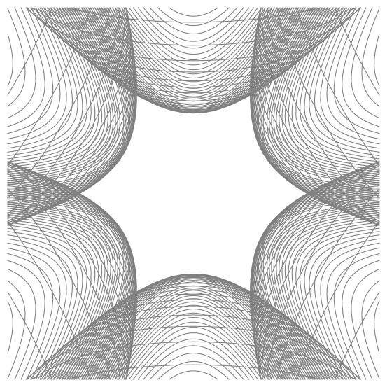
Figure 1.3: $P(\mathcal{H})$ in the 3-dimensional case

Local extremality with respect to Conjecture 1.26 is defined usually. Locally extremal matrices (and ellipsoids) are characterised via the following theorem; note that the result holds for lower dimensional extremal cases as well.

Theorem 1.27.

Assume that the ellipsoid $\mathcal{E}^{*}$, given by $x^{\top}M^{-1}x=n$, is locally extremal with respect to Conjecture 1.22. Let $(u_{i}^{-1})_{1}^{m}$ be the set of contact points between $\mathcal{E}^{*}$ and $\mathcal{H}$. Then there exist a series of positive numbers $(c_{i})_{1}^{m}$, such that

$$P(M)=\sum_{1}^{m}c_{i}\,P(u_{i})\otimes P(u_{i}^{-1}).$$ (1.49)

• If $\mathcal{E}^{*}$ is locally extremal, then $P(\mathcal{E}^{*})$ is locally extremal in $P(\mathcal{H})$ as well. The set of contact points between $P(\mathcal{E}^{*})$ and $P(\mathcal{H})$ are $(P(u_{i}^{-1}))$. Moreover, the duality relation implies that the normal direction to $\mathcal{H}$ at $u_{i}$ is parallel to $u_{i}^{-1}$, and accordingly, the normal to $P(\mathcal{H})$ at $P(u_{i})$ is parallel to $P(u_{i}^{-1})$.

We are going to use a different optimisation argument as in the proof of Theorem 1.24; the advantage is that this approach automatically works for lower dimensional extremal ellipsoids as well, therefore, there will be fewer assumptions on the separating matrix $H$. Moreover, $H$ will not be required to be symmetric either.

In order to move the ellipsoid $P(\mathcal{E}^{*})$ so that it stays in $P(\mathcal{H})$, the original contact points cannot cross the local separating hyperplanes. Since the matrix $P(M)$ is symmetric and positive semi-definite, it has a symmetric, positive semi-definite square-root $A$, for which $P(\mathcal{E}^{*})=A\,B_{2}^{n}$. Let $H$ be an arbitrary $n\times n$ matrix. We modify the matrix $A$ to $(I+\delta H)A$, where $\delta>0$. The image of the contact point $P(u_{i}^{-1})$ is $P(u_{i}^{-1})+\delta HP(u_{i}^{-1})$. Then $P(M)$ is modified to

$$((I+\delta H)A)^{2}=P(M)+\delta HP(M)+\delta AHA+\delta^{2}HAHA.$$

The derivative of the above expression with respect to $\delta$ at $\delta=0$ is $HP(M)+AHA$. Therefore, if the trace increases for small $\delta$, then

$$\mathrm{tr\,}HP(M)+\mathrm{tr\,}AHA=2\mathrm{tr\,}HP(M)>0.$$

On the other hand, if the image of $P(\mathcal{E}^{*})$ stays in the bounding box determined by the separating hyperplanes at the contact points, then for every $i$,

$$\langle P(u_{i}),P(u_{i}^{-1})+\delta HP(u_{i}^{-1})\rangle\leqslant\langle P(u_{i}),P(u_{i}^{-1})\rangle=n.$$

Therefore, if $\mathcal{E}^{*}$ is locally extremal, then there is no real $n\times n$ matrix $H$, for which

$$\langle P(u_{i}),HP(u_{i}^{-1})\rangle\leqslant 0$$

for every $i$, and

$$\mathrm{tr\,}HP(M)>0.$$

The only fact we need is that for two vectors $x,y\in\mathbb{R}^{n}$,

$$\langle Hx,y\rangle=\langle H,x\otimes y\rangle,$$

where the inner product of matrices is defined by (1.40). Therefore, $P(M)$ is not separable from the matrices $P(u_{i})\otimes P(u_{i}^{-1})$ by a linear functional, which implies that

$$P(M)\in\mathrm{pos\,}\{P(u_{i})\otimes P(u_{i}^{-1})\}\,.\quad\hbox{\leavevmode\hbox to7.77786pt{\hfil\vrule\vbox to6.75003pt{\hrule width=6.00006pt\vfil\hrule}\vrule\hfil}}$$

Note that in the above representation of $P(M)$, the traces of the matrices are $n$:

$$\mathrm{tr\,}P(u_{i})\otimes P(u_{i}^{-1})=\langle P(u_{i}),P(u_{i}^{-1})\rangle=n.$$

Hence it would suffice to show that for the coefficients in (1.49),

$$\sum c_{i}\leqslant\frac{n-1}{n}\,.$$

If $M$ is not singular, then we obtain the result which is analogous to Theorem 1.24.

Corollary 1.28.

The only non-degenerate ellipsoid $\mathcal{E}^{*}$, that is locally extremal with respect to Conjecture 1.26, is the unit ball $B_{2}^{n}$.

• We shall use that for $x,y\in\mathbb{R}^{n}$ and a real symmetric $n\times n$ matrix $A$,

  $$(x\otimes y)A=x\otimes(Ay).$$

  Assume that $M$ is not singular, and multiply both sides of (1.49) by $P(M^{-1})$. Then $P(M^{-1})P(u_{i}^{-1})=P(u_{i})$, and by (1.47), we obtain that

  $$I_{n}-\frac{\mathbf{1}\otimes\mathbf{1}}{n}=\sum c_{i}P(u_{i})\otimes P(u_{i}).$$ (1.50)

  Since $B_{2}^{n}\subset\mathrm{int}\mathcal{H}$, the norm of every point of $P(\mathcal{H})$ is at least $\sqrt{n}$. Therefore,

  $$\mathrm{tr\,}P(u_{i})\otimes P(u_{i})=\langle P(u_{i}),P(u_{i})\rangle\geqslant n.$$

  On the other hand,

  $$\mathrm{tr\,}\bigg{(}I_{n}-\frac{\mathbf{1}\otimes\mathbf{1}}{n}\bigg{)}=n-1.$$

  Thus, (1.50) implies that $\sum c_{i}\leqslant(n-1)/n$.         

If $M$ is singular, then proceeding the above way, instead of obtaining a representation of the projection onto $\mathbf{1}^{\perp}$, we derive a representation of the projection onto the subspace of $P(\mathcal{E}^{*})$. The problem is that we cannot estimate the norms of vectors in this subspace; moreover, in the lower dimensional extremal spaces, the norms of the contact points are not equal. Some relation connected to the scaling is missing. However, the fact that the characterisation of Theorem 1.27 works for any extremal case, give us hope that this approach for the polarization problems will eventually reach its goal.

Chapter 2 The problem of the longest convex chains

We discuss the following problem. Let $T$ be the triangle with vertices $(1,0),(0,0)$ and $(0,1)$. Choose $n$ independent, uniform random points from $T$, the collection of which is denoted by $X_{n}$. A subset $Y\subset X_{n}$ is a convex chain, if the points are the vertices of a convex path from $(0,1)$ to $(1,0)$. We are interested in the behaviour of the longest convex chains, where length is measured by the number of vertices. The maximal length is denoted by $L_{n}$. In Section 2.3, we prove an asymptotic result for the expectation of $L_{n}$. It turns out that $L_{n}$ is highly concentrated about its mean; this is the main content of Section 2.4. With the aid of this property, we show that the longest convex chains are in a small neighbourhood of a special parabolic arc with high probability. The proof of this theorem, that is presented in Section 2.6, is based on a conditional probabilistic method, to be found in Section 2.5. Finally, Section 2.7 contains numerical results obtained by computer simulations.

Most of these results were published in the joint article with Imre Bárány [3]. However, the material has been almost completely reorganised, and besides other modifications, the limit shape result is proven by a new method. Hopefully, these changes led to a more clarified exposition of the topic.

2.1 Introduction and related results

The area of probabilistic discrete geometry has a history that is almost 150 years old. In 1864, Sylvester posed the following problem in the Educational Times: “Show that the chance of four points forming the apices of a reentrant quadrilateral is 1/4 if they be taken at random in an indefinite plane”. It turned out immediately that the problem was wrongly formulated, as the underlying distribution on the plane was not specified. There are several ways to correct the question, the most popular of which has been the following: “Let $K$ be a convex body in the plane, and $n$ points independently from $K$ with uniform distribution. What is the probability that they are in convex position?” This question was fully answered by Bárány in 1999 [14]. The situation of choosing finitely many, independent, uniform random points in a convex body has been extremely fertile, and hundreds of papers have been written on related questions. For an excellent survey of some topics in the area, see e.g. Bárány [15].

In the present chapter we consider the following problem. Let $T\subset\mathbb{R}^{2}$ be a triangle with vertices $p_{0},p_{1},p_{2}$ and let $X=X_{n}$ be a random sample of $n$ independently chosen random points from $T$ with uniform distribution. A subset $Y\subset X_{n}$ is a convex chain in $T$ (from $p_{0}$ to $p_{2}$) if the convex hull of $Y\cup\{p_{0},p_{2}\}$ is a convex polygon with exactly $|Y|+2$ vertices. A convex chain $Y$ gives rise to the polygonal path $C(Y)$ which is the boundary of this convex polygon minus the edge between $p_{0}$ and $p_{2}$. The length of the convex chain $Y$ is just $|Y|$. We shall investigate the length of a longest convex chain in $X_{n}$, which will be denoted by $L_{n}$.

An equally plausible and natural question would be the following. Let $K$ be an arbitrary convex region in the plane, and choose $n$ random, uniform, independent points from $K$. What is the expectation of the largest subset of the random points in convex position? We will explain later in the section, that using standard methods, this question immediately boils down to the one above for triangles. We mainly chose to work with the random variable $L_{n}$ because of the similarity to the famous problem of the longest increasing subsequences in random permutations.

This connection is easily established. Indeed, let $X_{n}$ is a uniform sample of $n$ independent points from the unit square, and call a chain from $(0,0)$ to $(1,1)$ monotone, if the slope of every edge in it is positive. By ordering the points of $X_{n}$ according to their $x$-coordinates, the order of their $y$-coordinates represents a permutation $\sigma$ of $\{1,\dots,n\}$, where the longest monotone chain from $X_{n}$ corresponds to the longest increasing subsequence of $\sigma$. It is easy to check that the resulted distribution on $S_{n}$ is the uniform distribution.

The problem of the longest increasing subsequences is over 40 years old, in which period, it has been linked to various parts of mathematics, e.g. Young tableaux, patience sorting, planar point processes, and the theory of random matrices. In 1977, independently of each other, Logan and Shepp [29] and Vershik and Kerov [43] proved that the expectation is $2\sqrt{n}(1+o(1))$. After a variety of related results, the limit distribution was determined by Baik, Deift and Johansson in 1999 [7]. Surprisingly, this turned out to be the same as the limit distribution of the largest eigenvalue of random $n\times n$ Hermitian matrices, which was determined by Tracy and Widom in 1994 [41]. More details about the problem can be found in the excellent survey paper by Aldous and Diaconis [1].

Let us return now to random points in a planar convex body. We need some notation to formulate the results. The (Lebesgue) area of $K$ will be denoted by $A(K)$. Next, we define the affine perimeter of a planar convex body $S$, see e.g. [13] or [17]; there are many ways to do it, of which we choose the one which is most relevant. Choose a partition $x_{1},\dots,x_{m},x_{m+1}=x_{1}$ of the boundary $\partial S$, and for every $i$, let the line $l_{i}$ support $S$ at $x_{i}$. Denote by $T_{i}$ the triangle enclosed by $l_{i}$, $l_{i+1}$, and the segment $x_{1}\,x_{i+1}$. The affine perimeter of $S$ is then defined by

$$AP(S)=2\lim\sum_{1}^{m}\sqrt[3]{A(T_{i})},$$ (2.1)

where the limit is taken over a sequence of partitions whose mesh tends to 0. The existence of the limit is showed in the above cited papers. We also mention that if the boundary of $S$ is twice differentiable, then $AP(S)=\int_{\partial S}\kappa^{1/3}ds$, where $\kappa$ denotes the curvature of $\partial S$ and the integral is taken with respect to the arc length. Naturally, the affine length can be defined in the same manner for convex curves. Finally, for a convex body $K\subset\mathbb{R}^{2}$, let

$$A^{*}(K)=\sup\{AP(S):S\subset K\textrm{ convex}\}.$$ (2.2)

Because of compactness, the supremum in the above definition is attained. Furthermore, Bárány proved in [13] the maximiser is unique: there is exactly one convex body contained in $K$, say $K_{0}$, for which $A^{*}(K)=AP(K_{0})$. Now, the structure of $K_{0}$ is well known as well [13]. If $T$ is the triangle with vertices $p_{0},p_{1},p_{2}$, then among all convex curves connecting $p_{0}$ and $p_{2}$ within $T$, the unique parabola arc $\Gamma\subset T$ that is tangent to the sides $p_{0}p_{1}$ at $p_{0}$ and $p_{1}p_{2}$ at $p_{2}$ has the largest affine length. The parabola arc $\Gamma$ will be called the special parabola in $T$, see Figure 2.1. From this fact, it simply follows that $\partial K_{0}\setminus\partial K$ consists of parabola arcs that are tangent to $\partial K$ at their endpoints.

Figure 2.1: The special parabola

The importance of affine perimeter was first pointed out in the work of Rényi and Sulanke [35]. They proved that if $K$ is a smooth convex body in the plane, and $X_{n}$ is a uniform sample of $n$ points in $K$, then the expected number of the vertices of $\mathrm{conv}X_{n}$ (the convex hull of $X_{n}$) is asymptotically

$$\Gamma\left(\frac{5}{3}\right)\sqrt[3]{\frac{2}{3}}\left(A(K)\right)^{-1/3}AP(K)\,\sqrt[3]{n}.$$ (2.3)

Here of course $\Gamma$ stands for the Gamma function.

Now, let $K\subset\mathbb{R}^{2}$ be an arbitrary convex body. Bárány [14] proved that if we take all the convex polygons spanned by points of $X_{n}$, then the majority of them is close to $K_{0}$. Therefore, $K_{0}$ is the limit shape of the random convex polygons inside $K$. In the article [16], strengthening this result, an almost sure limit theorem and a central limit theorem for convex chains are proved.

Next, we give an alternative model for obtaining a sample from $K$, by choosing lattice points. The connection between this and the uniform model motivates a strong inspiration on both sides. Consider the lattice $(1/t)\,{\mathbb{Z}}^{2}$, where ${\mathbb{Z}}^{2}$ is the usual integer lattice in $\mathbb{R}^{2}$ and $t>0$ is large, and set $X=K\cap(1/t)\,{\mathbb{Z}}^{2}$. The same questions can be formulated for $X$ as for $X_{n}$. For instance, Andrews [5] proved an upper estimate for the number of vertices of the integer convex hull:

$$|\mathrm{conv}X|\leqslant c\,A(K)^{1/3}$$

for some constant $c$. This shows that the two models do not behave necessarily in the same way. However, for the convex lattice polytopes of $X$, the same limit shape result holds as for the uniform model. This, in full generality, was proved in [13].

Regarding the present problem, there exists a result about convex lattice chains. Let $T$ be the usual triangle, and consider the lattice points in $T$. Let $n=|X|$; clearly, for large $t$, $n\approx\mathrm{A}(T)\,t^{2}$. Write $Y_{n}\subset X$ for a longest convex chain in $T$. It is shown by Bárány and Prodromou [17] that, as $t\to\infty$ (or $n\to\infty$),

$$|Y_{n}|=\frac{6}{(2\pi)^{2/3}}\sqrt[3]{t^{2}\mathrm{A}(T)}(1+o(1))=\frac{6}{(2\pi)^{2/3}}n^{1/3}(1+o(1)).$$ (2.4)

Next, we list our results. First, in Section 2.3, we prove an asymptotic result about the expectation of $L_{n}$. In view of (2.4), we expect the order of magnitude to be $n^{1/3}$. This is indeed so:

Theorem 2.1.

There exists a positive constant $\alpha$, for which

$$\lim_{n\rightarrow\infty}\frac{\mathbb{E}L_{n}}{\sqrt[3]{n}}=\alpha\,.$$

We also establish the estimates $1.57<\alpha<3.43$. Numerical experiments suggest that $\alpha=3$ and we venture to conjecture that this is the actual value of $\alpha$, which would nicely match the expectation of the longest increasing subsequences.

We have seen that the convex chains are located close to the parabolic arc $\Gamma$ in both the uniform and the lattice models. Although this does not imply that the longest convex chains are close to $\Gamma$, it is reasonable to guess so. Indeed, we will essentially prove that if $\mathcal{C}(X_{n})$ is the collection of all longest convex chains from $X_{n}$, then for every $\varepsilon>0$,

$$\lim_{n\to\infty}\mathbb{P}\big{(}\textrm{dist}(C(Y),\Gamma)>\varepsilon\mbox{ for some }Y\in\mathcal{C}(X_{n})\,\big{)}=0,$$ (2.5)

where $\textrm{dist}(.,.)$ stands for the Hausdorff distance. In order to achieve this result, we need strong concentration results in the sense of Talagrand’s inequality, that are established in Section 2.4. Sections 2.5 and 2.6 contain the proof of the following quantitative limit shape theorem.

Theorem 2.2.

Let $\gamma\geqslant 1$ and define $\varepsilon=2\gamma^{1/2}\,n^{-1/12}(\log n)^{1/4}$. Then there exists $N>0$, depending on $\gamma$, such that for every $n>N$,

$$\mathbb{P}\big{(}{\rm dist}(C(Y),\Gamma)>\varepsilon\mbox{ for some }Y\in\mathcal{C}(X_{n})\big{)}<n^{-\gamma^{2}/14}.$$

Note that this is much stronger than (2.5), since here $\varepsilon\rightarrow 0$ as well.

Once Theorems 2.1 and 2.2 for triangles are known, it is not too hard to extend the results for arbitrary convex sets: the method is illustrated for example in [17]. We give a sketch here. Let $K\subset\mathbb{R}^{2}$ be a convex body, and $K_{0}$ its convex subset of maximal affine perimeter. Let $X_{n}$ be a uniform sample from $K$, and assume that $Y_{n}$ is a largest subset of $X_{n}$ in convex position. Let $C(Y_{n})$ be the polygonal path of $Y$. Let $m$ be fixed, and for every $k=1,\dots,m$, let $l_{k}$ be a tangent to $C(Y_{n})$ of direction $2\pi k/m$, with contact point $x_{k}$. Let $T_{k}$ be the triangle delimited by $l_{k}$, $l_{k+1}$, and the segment $x_{k}\,x_{k+1}$. It is easy to check that $Y_{n}\cap T_{k}$ is a maximal convex chain in $T_{k}$. For $n\gg m$, the number of points in $T_{k}$ is about $nA(T_{k})/A(K)$, and by Theorem 2.1 and formulae (2.1) and (2.2),

$$|Y_{n}|\approx\frac{\alpha\,n^{1/3}}{\sqrt[3]{A(K)}}\sum_{1}^{m}\sqrt[3]{A(T_{k})}\leqslant\frac{\alpha\,n^{1/3}A^{*}(K)}{2\sqrt[3]{A(K)}},$$

where $\alpha$ is the constant from Theorem 2.1. On the other hand, by choosing the points $x_{1},\dots,x_{m}$ on $\partial K_{0}$, the quantity on the right hand side can be achieved. Therefore,

$$\lim_{n\rightarrow\infty}n^{-1/3}\mathbb{E}|Y_{n}|=\frac{\alpha\mathrm{A}^{*}(K)}{2\root 3 \of{A(K)}}.$$

Moreover, this is achieved only if $C(Y)$ is sufficiently close to $K_{0}$; therefore, the limit shape of the maximal convex polygons is necessarily $K_{0}$.

The above argument serves as the basis for the subsequent proofs as well. However, there are many non-trivial details, and tricky proofs, to come.

Finally, we mention another model, that is often used in probabilistic geometry, although in the present case it will not be applied. Let $X(n)$ be a homogeneous planar Poisson process of intensity $n/\mathrm{A}(T)$. Given a domain $D$ in the plane, the number of points of $X(n)$ in $D$, that we denote by $m(D)$, has Poisson distribution with parameter $\lambda=n\mathrm{A}(D)/\mathrm{A}(T)$:

$$\mathbb{P}\big{(}m(D)=k\big{)}=e^{-\lambda}\lambda^{k}/k!\;.$$

We can also think of the Poisson model as follows: for a domain $D$, we first pick a random number $m$ according to the corresponding Poisson distribution, and then choose $m$ random, independent, uniform points in $D$. As is well known, the uniform model $X_{n}$ and the Poisson model $X(n)$ behave very similarly. In particular, Theorems 2.1, 2.2, and 2.8 remain valid for the latter as well, with essentially the same quantitative estimates. Obtaining these results from the ones presented here is straightforward. An equally standard way is to prove the theorems for the Poisson model, and then transfer the results to the uniform model. The disadvantage of obtaining slightly weaker results is balanced by the fact that under the Poisson model, the number of points of $X(n)$ in two disjoint domains are independent random variables.

The longest increasing subsequence problem has been almost completely solved by now, see [1]. In this respect, our results only constitute the first, and perhaps the simplest steps in understanding the random variable $L_{n}$.

2.2 Geometric and probabilistic tools

When choosing a random point in the triangle $T$, the underlying probability measure is the normalized Lebesgue measure on $T$. Most of the random variables treated in this chapter (e.g. $L_{n}$) are defined on the $n$th power of this probability space, to be denoted by $T^{n}$. In this case $\mathbb{P}$ denotes the $n$th power of the normalized Lebesgue measure on $T$. Plainly, choosing $n$ independent random points in $T$, the number of points in any domain $D\subset T$ is a binomial random variable of distribution $B(n,\mathrm{A}(D)/\mathrm{A}(T))$, and the expected number of points in $D$ is $n\mathrm{A}(D)/\mathrm{A}(T)$.

For binomial random variables we have the following useful deviation estimates, which are relatives of Chernoff’s inequality, see [2], Theorems A.1.12 and A.1.13. If $K$ has binomial distribution with mean value $k>1$ and $c>0$, then

$$\mathbb{P}\big{(}K\leqslant k-c\sqrt{k\log k}\,\big{)}\leqslant k^{-c^{2}/2}.$$ (2.6)

On the other hand, for $c>1$,

$$\mathbb{P}\big{(}K\geqslant ck\big{)}\leqslant\left(\frac{e}{c}\right)^{ck}.$$ (2.7)

We will use (2.6) often, mainly with $c=1$.

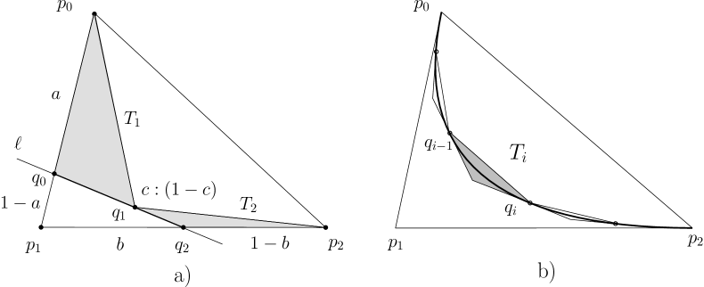
Figure 2.2: Characterisation of $\Gamma$

As we have mentioned earlier, the special parabola arc $\Gamma\subset T$ is characterized by the fact that it has the largest affine length among all convex curves connecting $p_{0}$ and $p_{2}$ within $T$. This is a consequence of the following theorem from [20]. Assume that a line $\ell$ intersects the sides $p_{0}p_{1}$ resp. $p_{1}p_{2}$ at points $q_{0}$ and $q_{2}$. Let $q$ be a point on the segment $q_{0}q_{2}$ and write $T_{1}$ resp. $T_{2}$ for the triangle with vertices $p_{0},q_{0},q$ resp. $q,q_{2},p_{2}$, see Figure 2.2 a).

Theorem 2.3 ([20]).

Under the above assumptions

$$\sqrt[3]{\mathrm{A}(T_{1})}+\sqrt[3]{\mathrm{A}(T_{2})}\leqslant\sqrt[3]{\mathrm{A}(T)}.$$

Equality holds here if and only if $q_{1}\in\Gamma$ and $\ell$ is tangent to $\Gamma$ at $q_{1}$.

The equality part of the theorem implies the following fact. Assume that $p_{0}=q_{0},q_{1},\dots,q_{k}=p_{2}$ are points, in this order, on $\Gamma$. Let $T_{i}$ be the triangle delimited by the tangents to $\Gamma$ at $q_{i-1}$ and $q_{i}$, and by the segment $q_{i-1}q_{i}$, $i=1,\dots,k$; see Figure 2.2 b).

Corollary 2.4.

Under the previous assumptions $\sum_{i=1}^{k}\sqrt[3]{\mathrm{A}(T_{i})}=\sqrt[3]{\mathrm{A}(T)}$. In particular, when $\mathrm{A}(T_{i})=t$ for each $i=1,\dots,k-1$ and $\mathrm{A}(T_{k})<t$, then $k-1\leq\sqrt[3]{\mathrm{A}(T)/t}<k$.

We will need a strengthening of Theorem 2.3. Assume $q_{0}$ resp. $q_{2}$ divides the segment $p_{0}p_{1}$ resp. $p_{1}p_{2}$ in ratio $a:(1-a)$ and $b:(1-b)$, see Figure 2.2 a).

Theorem 2.5.

With the above notation

$$\sqrt[3]{\mathrm{A}(T_{1})}+\sqrt[3]{\mathrm{A}(T_{2})}\leqslant\sqrt[3]{\mathrm{A}(T)}-\sqrt[3]{\mathrm{A}(T)}\frac{1}{3}(a-b)^{2}.$$

• Let $c$ be a number between $0$ and $1$, so that $q_{1}$ divides the segment $q_{0}q_{2}$ in ratio $c:(1-c)$. Then, writing $\mathrm{A}(xyz)$ for the area of the triangle with vertices $x,y,z$,

  $$\mathrm{A}(p_{0}q_{0}q_{1})=a\mathrm{A}(p_{0}p_{1}q_{1})=ac\mathrm{A}(p_{0}p_{1}q_{2})=abc\mathrm{A}(p_{0}p_{1}p_{2}),$$

  showing $\mathrm{A}(T_{1})=abc\mathrm{A}(T)$. Similarly, $\mathrm{A}(T_{2})=(1-a)(1-b)(1-c)\mathrm{A}(T).$ Hence we have to prove the following fact: $0\leqslant a,b,c\leqslant 1$ implies

  $$1-\sqrt[3]{abc}-\sqrt[3]{(1-a)(1-b)(1-c)}\geqslant\frac{1}{3}(a-b)^{2}.$$ (2.8)

  Denote $Q$ the left hand side of (2.8). By computing the derivative of $Q$ with respect to $c$ yields that for fixed $a$ and $b$, $Q$ is minimal when

  $$c=\frac{\sqrt{ab}}{\sqrt{ab}+\sqrt{(1-a)(1-b)}}\,.$$

  It is easy to see that with this $c$,

  $$\sqrt[3]{abc}+\sqrt[3]{(1-a)(1-b)(1-c)}=\left(\sqrt{ab}+\sqrt{(1-a)(1-b)}\right)^{2/3}.$$

  Now, denote $\left(\sqrt{ab}+\sqrt{(1-a)(1-b)}\right)^{2}$ by $1-u$, that is,

  $$u=a+b-2ab-2\sqrt{ab(1-a)(1-b)}.$$

  We claim that $u\geqslant(a-b)^{2}$: this is the same as

  $$a-a^{2}+b-b^{2}\geqslant 2\sqrt{(a-a^{2})(b-b^{2})},$$

  which is just the inequality between the arithmetic and geometric means for the numbers $a-a^{2},b-b^{2}\geq 0$. Therefore, using $u\leqslant 1$,

  $$Q\geqslant 1-(1-u)^{1/3}\geqslant\frac{1}{3}\,u\geqslant\frac{1}{3}\,(a-b)^{2}.\quad\hbox{\leavevmode\hbox to7.77786pt{\hfil\vrule\vbox to6.75003pt{\hrule width=6.00006pt\vfil\hrule}\vrule\hfil}}$$

Theorems 2.3 and 2.5 imply the following statement.

Corollary 2.6.

If $q\in\Gamma$ and $\ell$ is tangent to $\Gamma$ at $q$, then with the above notations, $a=b$.

Since an affine transformation does not influence the value of $L_{n}$, the underlying triangle $T$ can be chosen arbitrarily. Our standard model for $T$ is the one with $p_{0}=(0,1)$, $p_{1}=(0,0)$, $p_{2}=(1,0)$ as the vertices of $T$. In this case the special parabola $\Gamma$ is given by the equation $\sqrt{x}+\sqrt{y}=1$.

Finally, we will give strong concentration results for $L_{n}$ with the help of Talagrand’s following inequality [40]. Suppose that $Y$ is a real-valued random variable on a product probability space $\Omega^{\otimes n}$, and that $Y$ is 1-Lipschitz with respect to the Hamming distance, meaning that

$$|Y(x)-Y(y)|\leqslant 1$$

whenever $x$ and $y$ differ in one coordinates. Moreover assume that $Y$ is $f$-certifiable. This means that there exists a function $f:\mathbb{N}\rightarrow\mathbb{N}$ with the following property: for every $x$ and $b$ with $Y(x)\geqslant b$ there exists an index set $I$ of at most $f(b)$ elements, such that $Y(y)\geqslant b$ holds for every $y$ agreeing with $x$ on $I$. Let $m$ denote the median of $Y$. Then for every $s>0$ we have

$$\mathbb{P}(Y\leqslant m-s)\leqslant 2\,\mathrm{exp}\left(\frac{-s^{2}}{4f(m)}\right),$$ (2.9)

$$\mathbb{P}(Y\geqslant m+s)\leqslant 2\,\mathrm{exp}\left(\frac{-s^{2}}{4f(m+s)}\right).$$

2.3 Expectation

The aim of this section is to prove of Theorem 2.1. We also establish upper and lower bounds for the constant $\alpha$.

• We start with an upper bound on $\mathbb{E}L_{n}$:

  $$\limsup_{n\rightarrow\infty}\frac{\mathbb{E}L_{n}}{\sqrt[3]{n}}\leqslant\sqrt[3]{2}e=3.4248\dots.$$ (2.10)

  It is shown in [14], equation (5.3) (cf. [16] as well) that the probability of $k$ uniform independent random points in $T$ forming a convex chain is

  $$\frac{2^{k}}{k!\,(k+1)!}\;.$$

  Therefore we can estimate the probability that a convex chain of length $k$ exists:

  $$\mathbb{P}(L_{n}\geq k)\leq{n\choose k}\frac{2^{k}}{k!\,(k+1)!}\;.$$

  We use this estimate and Stirling’s formula to bound $\mathbb{E}L_{n}$. Assume $\gamma>\sqrt[3]{2}e$. Then

  $$\mathbb{E}L_{n} =\sum_{k=0}^{n}\mathbb{P}(L_{n}>k)\leqslant\sum_{k=0}^{n}\mathbb{P}(L_{n}\geq k)$$

  $$\leqslant\gamma\sqrt[3]{n}+\sum_{k>\gamma\sqrt[3]{n}}\mathbb{P}(L_{n}\geq k)$$

  $$\leqslant\gamma\sqrt[3]{n}+\sum_{k>\gamma\sqrt[3]{n}}{n\choose k}\frac{2^{k}}{k!\,(k+1)!}$$

  $$\leqslant\gamma\sqrt[3]{n}+\sum_{k>\gamma\sqrt[3]{n}}\frac{(2n)^{k}}{(k!)^{3}}$$

  $$\leqslant\gamma\sqrt[3]{n}+\sum_{k>\gamma\sqrt[3]{n}}\frac{1}{\sqrt{(2\pi\gamma)^{3}n}}\left(\frac{2\,e^{3}}{\gamma^{3}}\right)^{k}$$

  $$\leqslant\gamma\sqrt[3]{n}+n^{-1/2}C,$$

  where $C=\gamma^{3}/(\gamma^{3}-2e^{3})$ is a positive constant. Since this holds for arbitrary $\gamma>\sqrt[3]{2}\,e$, (2.10) is proved.

Next, we give a lower bound for $\mathbb{E}L_{n}$. We apply Corollary 2.4 with $t=2\mathrm{A}(T)/n$, obtaining a set of triangles $\{T_{1},\dots,T_{k}\}$, where for $1\leqslant i\leqslant k-1$, the area of $T_{i}$ is $t$, and the area of $T_{k}$ is less than $t$. By (2.4), $k\geqslant\sqrt[3]{n/2}$. Let $X_{n}$ be the uniform independent sample from $T$. Let $q_{i}$ be a point of $T_{i}\cap X_{n}$, provided that $T_{i}\cap X_{n}\neq\emptyset$. The collection of such $q_{i}$’s forms a convex chain. Hence, the expected length of the longest convex chain is at least the expected number of non-empty triangles $T_{i}$:

$$\mathbb{E}L_{n}\; \geqslant\;\sum_{1}^{k}\mathbb{P}\big{(}T_{i}\cap X_{n}\neq\emptyset\big{)}\;\geqslant\;(k-1)\left(1-\left(1-\frac{2}{n}\right)^{n}\right)$$

$$\geq\left(\sqrt[3]{\frac{n}{2}}-1\right)\,\left(1-e^{-2}\right)\approx 0.6862\,n^{1/3}.$$

What we have proved so far is that

$$\underline{\alpha}=\liminf_{n\rightarrow\infty}n^{-1/3}\mathbb{E}L_{n}>0.6862,\mbox{ and }\overline{\alpha}=\limsup_{n\rightarrow\infty}n^{-1/3}\mathbb{E}L_{n}<3.4249.$$

We show next that the limit exists. Suppose on the contrary that $\underline{\alpha}<\overline{\alpha}$.

The idea of the proof is to use Corollary 2.4 again with parameters chosen so that the expected length of the longest convex chains in the small triangles is close to $\overline{\alpha}$, while for the triangle $T$, $\mathbb{E}L_{n}$ is close to $\underline{\alpha}$. This will result in a contradiction.

Choose a large $n$ with $\mathbb{E}L_{n}\geqslant(1-\varepsilon)\,\overline{\alpha}\sqrt[3]{n}$, and an $N$ much larger than $n$ with $\mathbb{E}L_{N}\leq(1+\varepsilon)\,\underline{\alpha}\sqrt[3]{N}$. Here $\varepsilon$ is a suitably small positive number. Define $n_{1}$ by the equation $n=n_{1}-\sqrt{n_{1}\log n_{1}}$.

Choose $N$ uniform, independent random points from triangle $T$. Define $t=n_{1}/N$. Hence the expected number of points in a triangle of area $t$ (contained in $T$) is $n_{1}$.

Applying Corollary 2.4 with this $t$ yields the set of triangles $T_{1},\dots,T_{k}$, where $k>\sqrt[3]{N/n_{1}}$.

Denote by $k_{i}$ the number of points in $T_{i}$, and by $\mathbb{E}L^{i}$ the expectation of the length of the longest convex chain in $T_{i}$. Clearly, $k_{i}$ has binomial distribution with mean $n_{1}$, except for the last triangle where the mean is less than $n_{1}$.

Since the union of convex chains in the triangles $T_{i}$ is a convex chain in $T$ between $(0,0)$ and $(1,1)$, by the estimate (2.6) we have

$$\mathbb{E}L_{N} \geqslant\sum_{i\leqslant k}\mathbb{E}L^{i}\;\geq\;\sum_{i\leqslant k-1}\mathbb{P}(k_{i}>n)\mathbb{E}L_{n}$$

$$\geqslant\sum_{i\leqslant k-1}\left(1-n_{1}^{-1/2}\right)(1-\varepsilon)\,\overline{\alpha}\sqrt[3]{n}$$

$$\geqslant\left(\sqrt[3]{N/n_{1}}-1\right)\left(1-n_{1}^{-1/2}\right)(1-\varepsilon)\,\overline{\alpha}\sqrt[3]{n}$$

$$=\overline{\alpha}\,\sqrt[3]{N}(1-\varepsilon)\left(1-n_{1}^{-1/2}\right)\left(\sqrt[3]{n/n_{1}}-\sqrt[3]{n/N}\right)$$

$$\geq\overline{\alpha}\,\sqrt[3]{N}(1-2\varepsilon),$$

where the last inequality holds if $n$ is chosen large enough and $N$ is chosen even larger with $n/N$ very small. Thus $(1+\varepsilon)\,\underline{\alpha}\geq(1-2\varepsilon)\,\overline{\alpha}$ which, for small enough $\varepsilon$, contradicts our assumption $\underline{\alpha}<\overline{\alpha}$.         

The lower bound $\mathbb{E}L_{n}\geq 0.6862\,n^{1/3}$ is probably the easiest to prove. A better estimate, also mentioned by Enriquez [22], can be established by the following sketch. Assume $T$ is the standard triangle and let $D$ denote the domain of $T$ lying above $\Gamma$. Then $\mathrm{A}(D)=1/3$, so the expected number of points in $D$ is $2n/3$, and the number of points is concentrated around this expectation. The affine perimeter of $D$ is $2\sqrt[3]{1/2}$ (see [14]), and (2.3) yields that the expected number of vertices of $\mathrm{conv}(D\cap X_{n})$ is about

$$\Gamma\left(\frac{5}{3}\right)\sqrt[3]{\frac{2}{3}}\left(\frac{1}{3}\right)^{-1/3}2\sqrt[3]{1/2}\,\sqrt[3]{2n/3}\approx 1.5772\,\sqrt[3]{n}.$$

Since most vertices are located next to the parabola, the majority of them form a convex chain, and so

$$\liminf_{n\rightarrow\infty}\frac{\mathbb{E}L_{n}}{\sqrt[3]{n}}\geqslant 1.5772\dots.$$ (2.11)

This estimate leads to slightly stronger quantitative results, and thus from now on, we will use it instead of $\alpha>0.6862$.

2.4 Concentration results

In this section, we prove strong concentration results for $L_{n}$ and related variables. We will use Talagrand’s inequality (2.9), see Section 2.2. When applied to $L_{n}$, this yields a concentration result about the median, what we denote by $m_{n}$. However, we want to prove that $L_{n}$ is close to its expectation. Luckily, concentration ensures that the mean and the median are not far apart; in fact, it will turn out that $\lim n^{-1/3}m_{n}=\alpha$.

First, we need a lower bound on $m_{n}$.

Lemma 2.7.

Suppose that $\log n>25$. Then

$$m_{n}\geq\sqrt[3]{3n/\log n}.$$

Since this is a special case of Lemma 2.9, the proof will be given there.

Here comes our first, basic concentration result for $L_{n}$.

Theorem 2.8.

For every $\gamma>0$ there exists a constant $N$, such that for every $n>N$,

$$\mathbb{P}\big{(}|L_{n}-\mathbb{E}L_{n}|>\gamma\sqrt{\log n}\;n^{1/6}\big{)}<n^{-\gamma^{2}/14}.$$

• The statement cries out for the application of Talagrand’s inequality. The random variable $L_{n}$ satisfies the conditions with $f(b)=b$, since fixing the coordinates of a maximal chain guarantees that the length will not decrease, and changing one of the points changes the length of the maximal chain by at most one. Write $m=m_{n}$ for the median in the present proof. Setting $s=\beta\sqrt{m\log m}$ where $\beta$ is an arbitrary positive constant, (2.9) implies that

  $$\mathbb{P}\big{(}|L_{n}-m|\geqslant\beta\sqrt{m\log m}\,\big{)} <4\exp\left\{\frac{-\beta^{2}m\log m}{4(m+\beta\sqrt{m\log m})}\right\}$$

  $$=4\exp\bigg{\{}\frac{-\beta^{2}\log m}{4(1+\beta\sqrt{m^{-1}\log m})}\bigg{\}}$$

  Define now $\beta_{0}=c\sqrt{m/\log m}$ with a constant $c>0$, which will be specified at the end of the proof in order to give the correct estimate. If $\beta\leqslant\beta_{0}$, then $\beta\sqrt{m^{-1}\log m}\leq c$, and the denominator in the exponent is at most $4(1+c)$. Thus

  $$\mathbb{P}\big{(}|L_{n}-m|\geqslant\beta\sqrt{m\log m}\,\big{)}<4m^{\frac{-\beta^{2}}{4(1+c)}}.$$ (2.12)

  On the other hand, for $\beta>\beta_{0}$ we have

  $$\mathbb{P}\big{(}|L_{n}-m|\geqslant\beta\sqrt{m\log m}\,\big{)} <\mathbb{P}\big{(}|L_{n}-m|\geqslant\beta_{0}\sqrt{m\log m}\,\big{)}$$ (2.13)

  $$=4\exp\left(-m\,\frac{c^{2}}{4(1+c)}\right).$$

  Next, we compare the median and the expectation of $L_{n}$ using the following inequality:

  $$|\mathbb{E}L_{n}-m|\leqslant\mathbb{E}|L_{n}-m|=\int_{0}^{\infty}\;\mathbb{P}(|L_{n}-m|>x)dx.$$

  The range of $L_{n}$ is $[1,n]$, so the integrand is $0$ if $x>n$. Substitute $x=\beta\sqrt{m\log m}$, and divide the integral into two parts at $\beta_{0}$:

  $$|\mathbb{E}L_{n}-m|\leqslant 4\sqrt{m\log m}(I_{1}+I_{2}),$$

  where

  $$I_{1}=\int_{0}^{\beta_{0}}m^{-\beta^{2}/4(1+c)}d\beta<\int_{0}^{\infty}m^{-\beta^{2}/4(1+c)}d\beta=\sqrt{\frac{\pi(1+c)}{\log m}},$$ (2.14)

  and

  $$I_{2}=\int_{\beta_{0}}^{n/\sqrt{m\log m}}\exp\left(-m\,\frac{c^{2}}{4(1+c)}\right)d\beta<n\exp\left(-m\,\frac{c^{2}}{4(1+c)}\right).$$ (2.15)

  By Lemma 2.7, $n<m^{4}$, so $I_{2}<m^{4}\exp(-m\,c^{2}/4(1+c))$. Since $m_{n}$ goes to infinity as $n$ increases (again by Lemma 2.7), the bound on $I_{2}$ is eventually much smaller than the one on $I_{1}$:

  $$|\mathbb{E}L_{n}-m| \leqslant 4\sqrt{m\log m}(I_{1}+I_{2})$$

  $$<4\sqrt{\pi(1+c)m}+4\sqrt{m\log m}\,m^{4}\exp\left(-m\,\frac{c^{2}}{4(1+c)}\right)$$ (2.16)

  $$\leq 5\sqrt{\pi(1+c)}\sqrt{m}$$

  for all large enough $n$. Hence $\mathbb{E}L_{n}$ is of the same order of magnitude as $m_{n}$, and we obtain

  $$\lim n^{-1/3}\mathbb{E}L_{n}=\lim n^{-1/3}m_{n}=\alpha.$$ (2.17)

  For fixed $\gamma$ and for large enough $n$, (Proof) implies

  $$\mathbb{P}\big{(}|L_{n}-\mathbb{E}L_{n}|>\gamma\sqrt{\log n}\;n^{1/6}\big{)}$$

  $$\leqslant\mathbb{P}\big{(}|L_{n}-m|>\gamma\sqrt{\log n}\;n^{1/6}-|\mathbb{E}L_{n}-m|\,\big{)}$$

  $$\leqslant\mathbb{P}\big{(}|L_{n}-m|>\gamma\sqrt{\log n}\;n^{1/6}-5\sqrt{\pi(1+c)}\sqrt{m}\,\big{)}.$$

  Using $m_{n}\leq 3.43n^{1/3}$ from (2.10) and (2.17), it is easy to see that

  $$\gamma\sqrt{\log n}\;n^{1/6}-5\sqrt{\pi(1+c)\,m} \geq\gamma\sqrt{m}\left(\sqrt{\frac{3\log m-\log 41}{3.43}}-\frac{5\sqrt{\pi(1+c)}}{\gamma}\right)$$

  $$\geq\gamma\sqrt{\frac{3}{3.44}}\sqrt{m\log m}.$$

  Since for large enough $n$, $\gamma\sqrt{3/3.44}<\beta_{0}=c\sqrt{m/\log m}$, (2.12) finally implies

  $$\mathbb{P}\left(|L_{n}-\mathbb{E}L_{n}|\geqslant\gamma\sqrt{\log n}\;n^{1/6}\right)$$

  $$\leqslant\mathbb{P}\left(|L_{n}-m|\geq\gamma\sqrt{\frac{3}{3.44}}\sqrt{m\log m}\,\right)$$

  $$\leqslant 4m^{-3\gamma^{2}/13.76(1+c)}<n^{-\gamma^{2}/14,}$$

  where the last inequality follows from (2.17) and choosing $c=0.01$.         

We remark that the constant in the exponent is far from being the best possible, and we have made no attempt here to find its optimal value. In general, Talagrand’s inequality is too general to give the precise concentration, see Talagrand’s comments on this in [40]. Also, we note that the proof of Theorem 2.8 also yields the slightly stronger estimate $n^{-\gamma^{2}(1/14+\vartheta})$ for a sufficiently small $\vartheta$.

For the proof of Theorem 2.2 we need to consider subtriangles $S$ of $T$, that is, triangles of the form $S=\mathrm{conv}\;\{a,b,c\}$ with $a,b,c\in T$, while $X_{n}$ is still a random sample from $T$. We will need to estimate the concentration of the longest convex chain from $X_{n}$ in $S$. Since this random variable depends only on the relative area of $S$, we may and do assume that $T$ is the standard triangle and $S=\mathrm{conv}\{(0,\sqrt{s}),(0,0),(\sqrt{s},0)\}$. Thus $\mathrm{A}(S)=s/2$. Write $L_{s,n}$ for the length of the longest convex chain in $S$ from $(0,\sqrt{s})$ to $(\sqrt{s},0)$, and $m_{s,n}$ for its median. In the following statements, we consider the situation when $sn/2$, the expected number of points from $X_{n}$ in $S$, tends to infinity.

As in the proof of Theorem 2.8, we need two estimates: a lower bound for the median guarantees that the mean and the median are close to each other, while an upper bound for the expectation (or for the median) is needed to derive the inequality in terms of $n$. Here comes the lower bound; the case $s=1$ is Lemma 2.7.

Lemma 2.9.

Suppose that $\log(ns)>25$. Then

$$m_{s,n}\geq\sqrt[3]{3ns/\log(ns)}.$$

• Set $t=(\mathrm{A}(S)\log(ns))/(3ns)$, and apply Corollary 2.4 to the triangle $S$, resulting in the set of triangles $T_{1},\dots T_{k}$. Then for the number of triangles we have

  $$\sqrt[3]{3ns/\log(ns)}<k\leqslant\sqrt[3]{3ns/\log(ns)}+1.$$

  For any $i\in\{1,\dots,k$}, the probability that $T_{i}$ contains no point of $X_{n}$ is

  $$\mathbb{P}(T_{i}\cap X_{n}=\emptyset) \leqslant\left(1-\frac{\log(ns)}{3ns}\right)^{n}$$

  $$<\exp\left(\frac{-\log(ns)}{3s}\right)=(ns)^{-1/3s}<(ns)^{-1/3}.$$

  Hence the union bound yields

  $$\mathbb{P}\big{(}L_{n,s}>\sqrt[3]{3ns/\log(ns)}\,\big{)} \geq 1-\mathbb{P}(T_{i}\cap X_{n}=\emptyset\mbox{ for some }i\leq k)$$

  $$\geq 1-k\,(ns)^{-1/3}$$

  $$\geq 1-\big{(}\sqrt[3]{3/\log(ns)}+(ns)^{-1/3}\big{)},$$

  which is greater than $1/2$ by the assumption.         

Obtaining an upper bound for the mean is slightly more delicate; note that in the lemma below, $s$ need not be fixed.

Lemma 2.10.

Assume $ns\to\infty$. Then

$$\lim\,(ns)^{-1/3}\mathbb{E}L_{s,n}=\alpha$$

where $\alpha$ is the same constant as in Theorem 2.1.

• Take any $\varepsilon>0$ and choose $N_{0}$ (depending on $\varepsilon$) so large that for every $k\geqslant N_{0}$, $(1-\varepsilon)\alpha<\mathbb{E}L_{k}\,k^{-1/3}<(1+\varepsilon)\alpha$. The random variable $K=|X_{n}\cap S|$ has binomial distribution with mean $ns$. When $ns$ is large enough, $ns-\sqrt{ns\log ns}\geqslant N_{0}$, and we use (2.6) for a lower estimate:

  $$\mathbb{E}L_{s,n} =\sum_{k=0}^{n}\mathbb{P}(K=k)\mathbb{E}L_{k}$$

  $$\geqslant\mathbb{P}(K>ns-\sqrt{ns\log ns})(1-\varepsilon)\,\alpha\,(ns-\sqrt{ns\log ns})^{1/3}$$

  $$\geqslant(1-(ns)^{-1/2})(1-\varepsilon)\,\alpha\,(ns-\sqrt{ns\log ns})^{1/3}$$

  $$\geqslant(1-2\varepsilon)\,\alpha\,(ns)^{1/3}.$$

  For the upper bound, Jensen’s inequality applied to $\sqrt[3]{x}$ comes in handy:

  $$\mathbb{E}L_{s,n} =\sum_{k=0}^{n}\mathbb{P}(K=k)\mathbb{E}L_{k}$$

  $$\leqslant N_{0}\,\mathbb{P}(K<N_{0})+\sum_{k=N_{0}}^{n}\mathbb{P}(K=k)\mathbb{E}L_{k}$$

  $$\leqslant N_{0}\,+\sum_{k=N_{0}}^{n}\mathbb{P}(K=k)\,(1+\varepsilon)\,\alpha\,\sqrt[3]{k}$$

  $$\leqslant N_{0}\,+\mathbb{P}(K\geqslant N_{0})\,(1+\varepsilon)\,\alpha\,\left(\sum_{k=N_{0}}^{n}\frac{\mathbb{P}(K=k)}{\mathbb{P}(K\geqslant N_{0})}\ k\right)^{1/3}$$

  $$\leqslant N_{0}\,+\mathbb{P}(K\geqslant N_{0})^{2/3}\,(1+\varepsilon)\,\alpha\,(\mathbb{E}\,K)^{1/3}$$

  $$\leqslant N_{0}+(1+\varepsilon)\,\alpha\,(ns)^{1/3}\leqslant(1+2\varepsilon)\,\alpha\,(ns)^{1/3}.$$

Next, we derive the strong concentration property of $L_{s,n}$, the analogue of Theorem 2.8.

Theorem 2.11.

Suppose $\tau$ is a constant with $0\leqslant\tau<1$. Then for every $\gamma>0$ there exists a constant $N$, such that for every $n>N$ and every $s\geqslant n^{-\tau}$,

$$\mathbb{P}\big{(}|L_{s,n}-\mathbb{E}L_{s,n}|>\gamma\sqrt{\log ns}\;(ns)^{1/6}\big{)}<(ns)^{-\gamma^{2}/14}.$$

• This proof is almost identical with that of Theorem 2.8. Since $L_{s,n}$ is a random variable on $T^{\otimes n}$, we can apply Talagrand’s inequality with the certifying function $f(b)=b$ in the same way as in the proof of Theorem 2.8. Write again $m$ for $m_{s,n}$, the median of $L_{s,n}$. Define $\beta_{0}=c\sqrt{m/\log m}$ with $c=0.01$; then the estimates (2.12) and (2.13) remain valid with $L_{s,n}$ in place of $L_{n}$. Just as before,

  $$|\mathbb{E}L_{s,n}-m| \leqslant\mathbb{E}|L_{s,n}-m|=\int_{0}^{\infty}\;\mathbb{P}(|L_{s,n}-m|>x)dx$$

  $$=4\sqrt{m\log m}(I_{1}+I_{2})$$

  where $I_{1}$ and $I_{2}$ are defined the same way as in (2.14) and (2.15). Moreover, $I_{1}$ satisfies the inequality (2.14). With $I_{2}$ we have to be a bit more careful.

  Note that $s\geqslant n^{-\tau}$ with $\tau<1$ guarantees that Lemma 2.9 is applicable for $n>\exp(25/(1-\tau))$. As $x/\log x$ is monotone increasing for $x>e$,

  $$m\geq\sqrt[3]{\frac{3ns}{\log(ns)}}\geq\sqrt[3]{\frac{3n^{1-\tau}}{(1-\tau)\log n}}>\sqrt[3]{\frac{n^{1-\tau}}{n^{(1-\tau)/2}}}=n^{(1-\tau)/6}$$

  for large enough $n$, and therefore by (2.15)

  $$I_{2}<m^{6/(1-\tau)}\exp\left(-m\,\frac{c^{2}}{4(1+c)}\right)$$

  where of course $6/(1-\tau)<\infty$. Lemma 2.9 implies that $m=m_{s,n}\rightarrow\infty$, thus the bound on $I_{2}$ is much smaller than the one on $I_{1}$ for large enough $n$. Therefore, just as in (Proof),

  $$|\mathbb{E}L_{s,n}-m| \leqslant 4\sqrt{m\log m}(I_{1}+I_{2})$$

  $$<4\sqrt{\pi(1+c)m}+4\sqrt{m\log m}\,m^{6/(1-\tau)}\exp\left(-m\,\frac{c^{2}}{4(1+c)}\right)$$

  $$\leq 5\sqrt{\pi(1+c)}\sqrt{m}.$$

  Hence $\mathbb{E}L_{s,n}$ is of the same order of magnitude as $m=m_{s,n}$. Since $sn\geqslant n^{1-\tau}\rightarrow\infty$, we can use Lemma 2.10, yielding that for large enough $n$,

  $$m_{s,n}\leq 3.431\sqrt[3]{ns}.$$ (2.18)

  Again for fixed $\gamma$ and for large enough $n$,

  $$\mathbb{P}(|L_{s,n}-\mathbb{E}L_{s,n}|>\gamma\sqrt{\log ns}\;(ns)^{1/6})$$

  $$\leqslant\mathbb{P}(|L_{s,n}-m|>\gamma\sqrt{\log ns}\;(ns)^{1/6}-|\mathbb{E}L_{s,n}-m|)$$

  $$\leqslant\mathbb{P}(|L_{s,n}-m|>\gamma\sqrt{\log ns}\;(ns)^{1/6}-5\sqrt{\pi(1+c)}\sqrt{m}),$$

  and, by (2.18),

  $$\gamma\sqrt{\log ns}\;(ns)^{1/6}-5\sqrt{\pi(1+c)}\sqrt{m} \geq\gamma\sqrt{\frac{3}{3.44}}\sqrt{m\log m}.$$

  Since for large enough $n$, $\gamma\sqrt{3/3.44}<\beta_{0}=c\sqrt{m/\log m}$, (2.12) applied to $L_{s,n}$ and (2.18) finally implies

  $$\mathbb{P}\big{(}|L_{s,n}-\mathbb{E}L_{s,n}|\geqslant\gamma\sqrt{\log ns}\;(ns)^{1/6}\big{)}$$

  $$\leqslant\mathbb{P}\big{(}|L_{s,n}-m|\geq\gamma\sqrt{\frac{3}{3.44}}\sqrt{m\log m}\,\big{)}$$

  $$\leqslant 4m^{-3\gamma^{2}/13.76(1+c)}\leqslant(ns)^{-\gamma^{2}/14}.$$

We note that the proof also implies that for any $0<A<B<\infty$, there exists an $N$ (depending on $A$ and $B$ only), such that the inequality of Theorem 2.11 holds for any $\gamma\in[A,B]$ and for every $n>N$.

2.5 The conditional approach

Our proof of Theorem 2.2 is based on the following idea. Assume that $Y$ is a longest convex chain. Recall that $C(Y)$ is its convex polygonal path. Suppose that $C(Y)$ contains a point $q$ that is far from $\Gamma$, and let $\ell$ be a tangent line of $C(Y)$ at $q$. By Theorem 2.5 we know that if $T_{1}$ and $T_{2}$ denote the two triangles determined by $\ell$ and $q$, then $\sqrt[3]{\mathrm{A}(T_{1})}+\sqrt[3]{\mathrm{A}(T_{2})}$ is substantially smaller than $\sqrt[3]{1/2}$. Therefore, if $L^{i}$ denotes the length of the longest convex chain in $T_{i}$, then the expectation of $L^{1}+L^{2}$ is small as well, as it follows from the strong concentration property of the binomial distribution and Theorem 2.1. On the other hand, $C(Y)\subset T_{1}\cup T_{2}$, and hence $L^{1}+L^{2}$ is at least as large as $L_{n}$, whose expected value is – depending on the choice of the neighbourhood of $\Gamma$ – much larger than $\mathbb{E}(L^{1})+\mathbb{E}(L^{2})$. Therefore, either $L^{1}$, $L^{2}$, or $L_{n}$ is far from its expectation, which, according to the strong concentration results of the previous sections, has exponentially small probability.

The technical realisation of the above sketch is not trivial. One is tempted to proceed in the following way. Define the random variable $Z$ as the indicator function of the existence of a long convex chain:

$$Z=\Bigg{\{}\begin{array}[]{ll}1&\textrm{ if $L_{n}\geqslant\mathbb{E}L_{n}-\gamma\sqrt{\log n}\;n^{1/6}$}\\ 0&\textrm{ otherwise.}\end{array}$$

Recall that $\mathcal{C}(X_{n})$ is the collection of the longest convex chains in a given sample. The random variable $Q$ is defined as the (almost surely, unique) farthest point of $\bigcup\{C(Y):\ Y\in\mathcal{C}(X_{n})\}$ from $\Gamma$ in Euclidean distance.

Now, our aim is to show that if $q$ is “far” from $\Gamma$, then the conditional probability $\mathbb{P}(Z=1\,|\,Q=q)$ – or, what is the same, the conditional expectation of $Z$ – is exponentially small. At first glance, the area estimate of Theorem 2.5 plus the concentration results are sufficiently strong to derive this statement. However, some thinking reveals that this is not the case: since the condition on the farthest point modifies the underlying distribution, the previous results obtained for the uniform sample cannot be applied.

There are (at least) two ways to correct this reasoning. First, instead of estimating the conditional expectation in question at every point, we can use a finite approximation by estimating the (positive) probabilities that a longest convex chain intersects a small convex set far from $\Gamma$. This method was accomplished in our article [3]; it involves several tricks for choosing the right partitioning of $T$, and it reaches the goal via elementary, but tedious technical calculations.

For the purpose of the present thesis, a different method has been developed, still along the line of conditional probabilities. Note that the independence of the points of $X_{n}$ allows us to condition on the location of a point of the sample: the remaining $n-1$ points have the same joint distribution as $X_{n-1}$. Therefore we can estimate the probability of the existence of a long convex chain through a fixed point, given that the sample contains this point. This is the motivating idea.

By default, every result from now on is understood to hold when $n$ is large enough, where the bound on $n$ depends on $\gamma$ only. Also, with some ambiguity, we shall say that a convex chain contains a point, if its polygonal path contains it – it will be clear from the context if we require the point to be a vertex of the path.

Fix the constant $\gamma\geq 1$, and set

$$b=\gamma\,n^{1/6}\sqrt{\log n}.$$ (2.19)

We shall call a convex chain $Y\subset X_{n}$ long if its length is at least $\mathbb{E}L_{n}-b$. The strong concentration result of Theorem 2.8 directly shows that the probability of the existence of long chains is large:

$$\mathbb{P}(L_{n}<\mathbb{E}L_{n}-b)\leq n^{-\gamma^{2}/14}.$$ (2.20)

Figure 2.3: The parabola $\Gamma_{r}$

In measuring distances from $\Gamma$ it will be convenient to use the parabolic arcs

$$\Gamma_{r}=\{(x,y)\in T:\sqrt{x}+\sqrt{y}=\sqrt{1+r}\},$$

where $r\in(-1,1)$. Then $\Gamma_{0}=\Gamma$, and $\Gamma_{r}$ is the homothetic copy of $\Gamma$ with ratio of homothety $1+r$, and center of homothety at the origin, see Figure 2.3. Assume the point $(p,q)$ is on $\Gamma$. Then the point $\big{(}(1+r)\,p,(1+r)\,q\big{)}$ is on $\Gamma_{r}$, and the tangent line to $\Gamma_{r}$ at this point is given by the equation

$$\frac{x}{\sqrt{p}}+\frac{y}{\sqrt{q}}=1+r.$$ (2.21)

It follows that the distance between parallel tangent lines to $\Gamma$ and $\Gamma_{r}$ is

$$\frac{|r|}{\sqrt{1/p+1/q}}\leq\frac{|r|}{\sqrt{8}}.$$ (2.22)

Theorem 2.2 asserts that for a given $\gamma$, the longest convex chains are within the $\varepsilon$-neighbourhood of $\Gamma$ with probability $n^{-\gamma^{2}/14}$, where $\varepsilon=3/2\gamma^{1/2}\,n^{-1/12}(\log n)^{1/4}$. Define

$$\rho=\sqrt{8}\,\varepsilon=4\sqrt{2}\gamma^{1/2}n^{-1/12}(\log n)^{1/4}.$$ (2.23)

Formula (2.22) immediately implies that if a convex chain $C(Y)$ lies between $\Gamma_{-\rho}$ and $\Gamma_{\rho}$, then $\textrm{dist}(C(Y),\Gamma)\leq\varepsilon$. Therefore, in order to obtain Theorem 2.2, we shall prove that all the longest convex chains are between $\Gamma_{-\rho}$ and $\Gamma_{\rho}$ with large probability (meaning that the polygonal paths of the chains are in the required region).

For any point $q\in T$, we define the line $\ell(q)$ as the tangent to $\Gamma_{r}$ at $q$, where $r$ is the unique parameter such that $q\in\Gamma_{r}$.

Let $Y$ be a convex chain. By continuity and compactness, the set of $r$’s such that $C(Y)\cap\Gamma_{r}\neq\emptyset$ is a closed sub-interval $[r_{1},r_{2}]$ of $[-1,1]$. The set of lower extremal points of $C(Y)$ is defined by

$$\mathcal{E}_{l}(Y)=C(Y)\cap\Gamma_{r_{1}}\;,$$

and similarly, the set of upper extremal points of $C(Y)$ is given by

$$\mathcal{E}^{u}(Y)=C(Y)\cap\Gamma_{r_{2}}\;.$$

We shall simply call elements of $\mathcal{E}_{l}(Y)\cup\mathcal{E}^{u}(Y)$ extremal points of $Y$. Plainly, if $q$ is an extremal point, then $\ell(q)$ is a tangent to $C(Y)$, and $C(Y)\subset T_{1}\cup T_{2}$, where $T_{1}$ and $T_{2}$ are the triangles determined by $q$ and $\ell(q)$, see Figure 2.3 a). There are two cases: if $q$ is a lower extremal point, then by convexity, $q$ must be a vertex of $C(Y)$, that is, $q\in Y$. On the other hand, if $q$ is an upper extremal point, then there are two points $y_{1}$ and $y_{2}$ of $Y$ such that $q\in y_{1}y_{2}$, the segment between $y_{1}$ and $y_{2}$. We shall handle these cases separately.

For a point $q\in T$ with $q\in\Gamma_{\varrho}$, we naturally say that $q$ is below or above $\Gamma_{r}$ depending on whether $\varrho\leqslant r$ or $\varrho>r$. For a given $q\in T$, let $\ell(q)\in E(X_{n})$ denote the event that there are two points $p_{1},p_{2}\in X_{n}\cap\ell(q)$, for which $q\in p_{1}p_{2}$. We introduce the conditional probabilities $P(q)$ for $q\in T$ by

$$P(q)=\Bigg{\{}\begin{array}[]{ll}\mathbb{P}(\exists\textrm{ long convex chain $Y\subset X_{n}$ with $q\in\mathcal{E}_{l}(Y)$ $|$ $q\in X_{n}$})&\textrm{for $q$ below $\Gamma$;}\\ \mathbb{P}(\exists\textrm{ long conv. chain $Y\subset X_{n}$, $q\in\mathcal{E}^{u}(Y)$ $|$ $\ell(q)\in E(X_{n})$})&\textrm{for $q$ above $\Gamma$.}\end{array}$$

Let $S$ denote the subset of $T$ below $\Gamma_{-\rho}$ and $U$ denote the part of $T$ above $\Gamma_{\rho}$, where $\rho$ is given by (2.23). The next theorem provides a natural and essential link to the conditional probabilities $P(q)$, and it serves as the key to Theorem 2.2.

Theorem 2.12.

With the above notations,

$$\mathbb{P}(\exists\textrm{ long convex chain not} \textrm{ entirely between $\Gamma_{-\rho}$ and $\Gamma_{\rho}$})$$ (2.24)

$$\leqslant n\int_{S}P(q)d\mu(q)+10\,n^{2}\int_{U}P(q)d\mu(q),$$

where $\mu$ stands for the normalised Lebesgue measure on $T$.

• This is the moment to use a finite approximation. Let $\delta$ be a small positive number, and cover $T$ with a disjoint union of squares with axis-parallel sides of length $\delta$. The set of the squares in the cover is called $\mathscr{D}$. Now, the probability on the left hand side of (2.24) is certainly smaller than

  $$\sum_{D\in\mathscr{D}:D\cap S\neq\emptyset}\mathbb{P}(\exists\textrm{ long convex chain $Y\subset X_{n}$ with $D\cap\mathcal{E}_{l}(Y)\neq\emptyset$ })\\ +\sum_{D\in\mathscr{D}:D\cap U\neq\emptyset}\mathbb{P}(\exists\textrm{ long convex chain $Y\subset X_{n}$ with $D\cap\mathcal{E}^{u}(Y)\neq\emptyset$ })$$

  For squares $D\in\mathscr{D}$ intersecting $S$, the lower extremal point in $D$ is an element of $X_{n}$, and hence

  $$\mathbb{P}(\exists\textrm{ long convex chain $Y\subset X_{n}$ with }D\cap\mathcal{E}_{l}(Y)\neq\emptyset)$$

  $$=\mathbb{P}(\exists\textrm{ long convex chain }Y\subset X_{n},D\cap\mathcal{E}_{l}(Y)\neq\emptyset\ \textrm{and}\ X_{n}\cap D\neq\emptyset)$$

  $$=\mathbb{P}(\exists\textrm{ long convex chain }Y\subset X_{n},D\cap\mathcal{E}_{l}(Y)\neq\emptyset\ |\ X_{n}\cap D\neq\emptyset)\ \mathbb{P}(X_{n}\cap D\neq\emptyset).$$

  Here,

  $$\mathbb{P}(X_{n}\cap D\neq\emptyset)\leqslant 1-(1-2\delta^{2})^{n}\leqslant n\,2\,\delta^{2}=n\mu(D),$$ (2.25)

  and taking limits when $\delta\rightarrow 0$, we obtain the first term of the right hand side of (2.24).

Now, let $D\in\mathscr{D}$ intersect $U$. If $D$ contains an upper extremal point of a long convex chain, then there exists $q\in D$ and $p_{1},p_{2}\in X_{n}$, such that $p_{1},p_{2}\in l(q)$ and $q\in p_{1}p_{2}$. Let

$$\ell(D)=\bigcup\{\ell(q)\cap T:q\in D\}$$

be the “double cone” centred at $D$, see Figure 2.4 a). Then $\ell(D)\setminus D$ splits into two disjoint parts, that we call “left” and “right” parts. Let $D_{l}$ be the union of the left part with $D$, and similarly, $D_{r}$ be the union of the right part with $D$. As above,

$$\mathbb{P}(\exists\textrm{ long convex chain $Y\subset X_{n}$ with $D\cap\mathcal{E}^{u}(Y)\neq\emptyset$ })$$

$$=\mathbb{P}(\exists\textrm{ long conv. chain $Y\subset X_{n}$, $D\cap\mathcal{E}^{u}(Y)\neq\emptyset$, and }D_{l}\cap X_{n}\neq\emptyset,D_{r}\cap X_{n}\neq\emptyset)$$

$$\begin{aligned} =\mathbb{P}(\exists\textrm{ long conv. chain }Y\subset X_{n},D\cap\mathcal{E}^{u}(Y)\neq\emptyset\ |\ \exists q\in D:\ell(q)\in E(X_{n})\\ \cdot\,\mathbb{P}(D_{l}\cap X_{n}\neq\emptyset,D_{r}\cap X_{n}\neq\emptyset).\qquad\end{aligned}$$

By taking limits when $\delta\rightarrow 0$, the correlation of the events $D_{l}\cap X_{n}\neq\emptyset$ and $D_{r}\cap X_{n}\neq\emptyset$ tends to 0. Therefore, the proof will be completed as above if we show that

$$\mathbb{P}(D_{l}\cap X_{n}\neq\emptyset)\;\mathbb{P}(D_{r}\cap X_{n}\neq\emptyset)\leqslant 20\,n^{2}\delta^{2}$$

for every $D\in\mathscr{D}$ intersecting $U$. Similarly to (2.25),

$$\mathbb{P}(D_{l}\cap X_{n}\neq\emptyset)\;\mathbb{P}(D_{r}\cap X_{n}\neq\emptyset)\leqslant 4n^{2}A(D_{l})A(D_{r}),$$

and hence the inequality to prove is

$$A(D_{l})A(D_{r})\leqslant 5\,\delta^{2}\,.$$ (2.26)

Figure 2.4: Squares above $\Gamma$

Let the vertices of $D$ in counter-clockwise order be $(x,y)$, $(x,y+\delta)$, $(x-\delta,y+\delta)$ and $(x-\delta,y)$. It is easy to see that among the lines $\ell(q)$ with $q\in D$, the ones with extremal slopes are the ones belonging to $(x,y)$ and $(x-\delta,y+\delta)$. Let us call $p_{1}=(x,y)$, the lower right vertex, and $p_{2}=(x-\delta,y+\delta)$, the upper left vertex of $D$, see Figure 2.4 b). Let $\varphi$ be the slope of the ray $o\,p_{1}$, where $o$ is the origin. By symmetry, we may assume that $\varphi\leqslant\pi/2$.

Denote $\psi$ the angle between the rays $o\,p_{1}$ and $o\,p_{2}$. If $\delta$ is small enough, then both $p_{1}$ and $p_{2}$ are above $\Gamma$, and hence their distance from $o$ is at least $1/(2\sqrt{2}$). On the other hand, $|p_{1}p_{2}|=\sqrt{2}\delta$. Therefore

$$\psi\leqslant\arcsin 4\delta\approx 4\delta.$$ (2.27)

By formula (2.21), for any point $p$ on the ray $o\,p_{1}$, the lines $\ell(p)$ and $\ell(p_{1})$ are parallel, and their slope is

$$\nu(\varphi)=-\arctan(\sqrt{\tan\varphi}).$$

The slope of $\ell(p_{2})$ is $\nu(\varphi+\psi)$. Now,

$$\nu\,^{\prime}(\varphi)=-\frac{1}{2(\sin\varphi+\cos\varphi)\sqrt{\sin\varphi\cos\varphi}}\,.$$

As it can easily be checked, $\nu\,^{\prime}(\varphi)$ is a concave function, and $|\nu\,^{\prime}(\varphi)|\leqslant 1/\sqrt{2\sin 2\varphi}$. Therefore the angle between $\ell(p_{1})$ and $\ell(p_{2})$ is

$$\sigma=\nu(\varphi)-\nu(\varphi+\psi)\leqslant\frac{\psi}{\sqrt{2\sin 2\varphi}}\;.$$ (2.28)

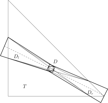
Figure 2.5: Covering $\ell(D)$ with a bow-tie

We divide the rest of the argument into two parts depending on the size of $\varphi$. If $\varphi>0.17$, then $1/\sqrt{2\sin 2\varphi}<1.23<\sqrt{5}-1$, and hence by (2.27),

$$\sigma\leqslant 4(\sqrt{5}-1)\,\delta.$$

Therefore $D_{l}\cup D_{r}$ can be covered with a “bow-tie”: the union of two oppositely placed trapezoids with shorter base length at most $\sqrt{2}\delta$, whose angle between the non-parallel opposite sides is less than $4(\sqrt{5}-1)\,\delta$, and the sum of their altitudes is at most $\sqrt{2}$, see Figure 2.5. A straightforward calculation reveals that under these conditions, $A(D_{l})A(D_{r})$ is maximal when both the altitudes are $1/\sqrt{2}$, and then

$$A(D_{l})A(D_{r})<5\,\delta^{2}.$$

Finally, when $\varphi\leqslant 0.17$, then $2\varphi/\sin 2\varphi\leqslant 1.02$, and hence (2.27) and (2.28) essentially imply that

$$\sigma\leqslant\frac{2\delta}{\sqrt{\varphi}}\;.$$

We shall justify the use of this estimate by leaving a sufficient gap at the end. Recall that $x$ and $y$ are the coordinates of the vertex $p_{1}$. Since $p_{1}$ is above $\Gamma$, they satisfy the inequality $\sqrt{x}+\sqrt{y}>1$. On the other hand, $\tan\varphi=y/x$. These relations immediately yield that

$$x\geqslant\frac{\cos\varphi}{\sqrt{\cos\varphi}+\sqrt{\sin\varphi}}\approx\frac{1}{1+\sqrt{\varphi}}\;.$$

Moreover, the slopes of the tangent lines $\ell(p_{1})$ and $\ell(p_{2})$ are at most $0.4$. Therefore, $D_{r}$ is covered by a trapezoid, whose shorter base is of length at most $1.1\delta$, the angle between its non-parallel opposite edges is at most $2\delta/\sqrt{\varphi}$, and its altitude is at most

$$1.1\left(1-\frac{1}{1+\sqrt{\varphi}}\right)\leqslant 1.1\sqrt{\varphi}.$$

Hence, $A(D_{r})\leqslant 2.5\,\delta\sqrt{\varphi}$. On the other hand, $D_{l}$ is covered by a trapezoid with shorter base-length $1.1\delta$, opening angle at most $2\delta/\sqrt{\varphi}$ and altitude at most $1.1$, therefore

$$A(D_{l})\leqslant 1.21\,\delta\left(1+\frac{1}{\sqrt{\varphi}}\right).$$

Altogether,

$$A(D_{r})A(D_{l})\leqslant 3.025(1+\sqrt{\varphi})\,\delta^{2}<4.3\,\delta^{2},$$

therefore (2.26) holds for sufficiently small $\delta$, and the proof is complete.         

2.6 Limit shape

In this section we finally prove Theorem 2.2. The first lemma formalises the intuitive idea that was presented at the beginning of Section 2.5. Let $q\in T$ be an arbitrary point, and as usual, let $T_{1}$ and $T_{2}$ denote the two triangles determined by $\ell(q)$ and $q$. Let $X_{n}$ be a random sample of $n$ points from $T$ and let $L^{i}$ denote the length of the longest convex chain in $T_{i}$, $i=1,2$.

Lemma 2.13.

For sufficiently large $n$, if $|r|\geq n^{-1/12}$, then

$$\mathbb{E}L^{1}+\mathbb{E}L^{2}\leq\mathbb{E}L_{n}-0.52\,r^{2}\sqrt[3]{n}.$$

• Let $t_{i}=\mu(T_{i})$ for $i=1,2$. We want to apply Theorem 2.5. It is not hard to see (using Corollary 2.6 for instance) that what is denoted by $|a-b|$ there, is equal to $|r|$ here. Consequently

  $$\sqrt[3]{t_{1}/2}+\sqrt[3]{t_{2}/2}\leqslant\sqrt[3]{1/2}-\sqrt[3]{1/2}\;\frac{1}{3}\,r^{2}.$$ (2.29)

  Write $L^{i}$ for the longest convex chain in the triangle $T_{i}$. By affine invariance, $L^{i}$ has the same distribution as $L_{t_{i},n}$ (from Section 2.4) for $i=1,2$. We need to estimate $\mathbb{E}L_{n}-(\mathbb{E}L^{1}+\mathbb{E}L^{2})$ from below.

  

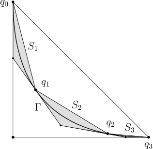
  Figure 2.6: Estimating the expectations

For four points $q_{0}=(0,1)$, $q_{1}$, $q_{2}$ and $q_{3}=(1,0)$ in this order on $\Gamma$, denote $S_{i}$ the triangle delimited by the tangents to $\Gamma$ at $q_{i-1},q_{i}$, and by the segment $q_{i-1}q_{i}$, $i=1,2,3$; see Figure 2.6. Choose $q_{1}$ and $q_{2}$ so that $\mathrm{A}(S_{1})=t_{1}/2$ and $\mathrm{A}(S_{2})=t_{2}/2$. Then Corollary 2.4 and (2.29) imply that

$$\sqrt[3]{\mathrm{A}(S_{3})}\geqslant\sqrt[3]{1/2}\;\frac{1}{3}\,r^{2}.$$

Let now $\Lambda^{i}$ denote the length of a longest chain in $S_{i}$ for $i=1,2,3$. For $i=1$ and $2$, $\Lambda^{i}$ has the same distribution as $L_{t_{i},n}$ (and as $L^{i}$). Therefore $\mathbb{E}L^{i}=\mathbb{E}L_{t_{i},n}=\mathbb{E}\Lambda^{i}$ for $i=1,2$. Further, $\Lambda^{1}+\Lambda^{2}+\Lambda^{3}\leq L_{n}$ follows from concatenating the longest convex chains in the triangles $S_{i}$. Thus we have

$$\mathbb{E}L^{1}+\mathbb{E}L^{2}+\mathbb{E}\Lambda^{3}=\sum_{i=1}^{3}\mathbb{E}\Lambda^{i}\leqslant\mathbb{E}L_{n}.$$ (2.30)

The random variable $|X_{n}\cap S_{3}|$ has binomial distribution with mean $2A(S_{3})n$ which is at least $\kappa=(1/3)^{3}r^{6}n\geq(1/3)^{3}n^{1/2}$. Set $N=\kappa-\sqrt{\kappa\log\kappa}$. Thus we obtain that for all large enough $n$,

$$N>0.99\,\kappa=\frac{0.99}{27}r^{6}n,$$

and $N$ tends to infinity with $n$. Using the estimates (2.6) and (2.11), again for large $n$ we have

$$\mathbb{E}\Lambda^{3} \geqslant\mathbb{P}(|X_{n}\cap S_{3}|\geqslant N)\,\mathbb{E}L_{N}\geqslant(1-\kappa^{-1/2})\ 1.57\,N^{1/3}$$

$$\geqslant 1.569N^{1/3}\geqslant 0.52\,r^{2}\sqrt[3]{n}.$$

Hence, by (2.30)

$$\mathbb{E}L^{1}+\mathbb{E}L^{2}\leqslant\mathbb{E}L_{n}-0.52\,r^{2}\sqrt[3]{n}.$$

Next, we estimate the conditional probabilities $P(q)$ from Section 2.5 for points $q$ that are far from $\Gamma$.

Lemma 2.14.

For any fixed $\gamma>0$, there exists an $N$, such that for every $n>N$,

$$P(q)\leqslant n^{-31\gamma^{2}/14}$$

for every $q$, that is below $\Gamma_{-\rho}$ or above $\Gamma_{\rho}$.

• Assume that $Y$ is a long convex chain that contains $q$. If $q$ is below $\Gamma_{-\rho}$, then $X_{n}\setminus q$ is distributed as $X_{n-1}$. Therefore if $\tilde{L}^{1}$ and $\tilde{L}^{2}$ denote the length of the longest convex chains in $T_{1}$ and $T_{2}$, then $\tilde{L}^{i}$ is distributed as $L_{t_{i},n-1}$ for $i=1,2$, where $t_{i}=\mu(T_{i})$. Moreover, $|Y\cap T_{i}|\leqslant\tilde{L}^{i}$. Recall that, since $Y$ is a long convex chain, its length is at least $\mathbb{E}L_{n}-b$, where $b$ is given by (2.19). Thus,

  $$\mathbb{E}L_{n}-b\leqslant|Y|\leqslant|Y\cap T_{1}|+|Y\cap T_{2}|\leqslant\tilde{L}^{1}+\tilde{L}^{2}+1.$$

  Therefore,

  $$P(q)\leqslant\mathbb{P}(\tilde{L}^{1}+\tilde{L}^{2}+1\geqslant\mathbb{E}L_{n}-b).$$

  Since $n,b\rightarrow\infty$, the term “$+1$” makes no difference at the estimates. Furthermore, $\mathbb{P}(\tilde{L}^{1}+\tilde{L}^{2}\geqslant\mathbb{E}L_{n}-b)\leqslant\mathbb{P}(L^{1}+L^{2}\geqslant\mathbb{E}L_{n}-b)$, and hence

  $$P(q)\leqslant\mathbb{P}(L^{1}+L^{2}\geqslant\mathbb{E}L_{n}-b).$$ (2.31)

  When $q$ is above $\Gamma_{\rho}$, then there are two points $y_{1},y_{2}\in X_{n}$ on $l(q)$ such that $q\in y_{1}y_{2}$, and $Y$ is contained in the triangles $\tilde{T}_{1}$ and $\tilde{T}_{2}$ determined by $\ell(q)$, $y_{1}$ and $y_{2}$. Now, $X_{n}\setminus\{y_{1},y_{2}\}$ is distributed as $X_{n-2}$, and $\tilde{T}_{1}\subset T_{1}$, $\tilde{T}_{2}\subset T_{2}$. Therefore a similar reasoning as above results in (2.31).

  Lemma 2.13, (2.19) and (2.23) gives that

  $$\mathbb{E}L^{1}+\mathbb{E}L^{2}\leqslant\mathbb{E}L_{n}-0.52\,\rho^{2}n^{1/3}<\mathbb{E}L_{n}-13b,$$

  therefore

  $$P(q) \leqslant\mathbb{P}(L^{1}+L^{2}\geqslant\mathbb{E}L_{n}-b)$$ (2.32)

  $$\leqslant\mathbb{P}(L^{1}+L^{2}\geqslant\mathbb{E}L^{1}+\mathbb{E}L^{2}+12b)$$

  $$\leqslant\sum_{i=1,2}\mathbb{P}(L^{i}\geq\mathbb{E}L^{i}+6b).$$

  Next, we estimate $\mathbb{P}(L^{i}\geq\mathbb{E}L^{i}+6b)$. When $t_{i}=2A(T_{i})\geq n^{-5/6}$, we use Theorem 2.11 with $\tau=5/6$:

  $$\mathbb{P}(L^{i}\geq\mathbb{E}L^{i}+6b)=\mathbb{P}(L^{i}\geqslant\mathbb{E}L^{i}+6\gamma\sqrt{\log n}\;n^{1/6})$$

  $$\leqslant\mathbb{P}(L^{i}\geqslant\mathbb{E}L^{i}+6\gamma\sqrt{\log n/\log(nt_{i})}\,\sqrt{\log(nt_{i})}\;(nt_{i})^{1/6})$$

  $$\leqslant(nt_{i})^{-\gamma^{2}36\log n/14\log(nt_{i})}=n^{-36\gamma^{2}/14}.$$

  The last inequality holds according to the remark following Theorem 2.11, since

  $$1\leqslant 6\gamma\sqrt{\log n/\log(nt_{i})}\leqslant\gamma\,6^{3/2}.$$

  Finally, when $t_{i}<n^{-5/6}$, the expected number of points in $T_{i}$ is $t_{i}n<n^{1/6}$. So for the random variable $|T_{i}\cap X_{n}|$ inequality (2.7) implies that

  $$\mathbb{P}\big{(}\,|T_{i}\cap X_{n}|\geqslant 6\gamma\sqrt{\log n}\;n^{1/6}\big{)} \leqslant\left(\frac{e\,t_{i}n}{6\gamma\sqrt{\log n}\;n^{1/6}}\right)^{6\gamma\sqrt{\log n}\;n^{1/6}}$$

  $$\leqslant\left(\frac{e}{6\gamma\sqrt{\log n}}\right)^{n^{1/6}} <n^{-32\gamma^{2}/14}$$

  for large enough $n$, as it can easily be seen by taking logarithms.

  Therefore, in both cases

  $$\mathbb{P}\big{(}L^{i}\geqslant\mathbb{E}L^{i}+6\,b\big{)}<n^{-32\gamma^{2}/14},$$

  and by (2.32),

  $$P(q)<2n^{-32\gamma^{2}/14}<n^{-31\gamma^{2}/14}.\quad\hbox{\leavevmode\hbox to7.77786pt{\hfil\vrule\vbox to6.75003pt{\hrule width=6.00006pt\vfil\hrule}\vrule\hfil}}$$

• We have to estimate the probability that there is a longest convex chain not lying between $\Gamma_{-\rho}$ and $\Gamma_{\rho}$. This event splits into two parts: either the longest convex chain has less than $\mathbb{E}L_{n}-b$ points, or there is a long convex chain not entirely between $\Gamma_{-\rho}$ and $\Gamma_{\rho}$. By Theorem 2.8 and the remark following it,

  $$\mathbb{P}(L_{n}<\mathbb{E}L_{n}-b)<n^{-\gamma^{2}(1/14+\vartheta)}$$

  for some positive $\vartheta>0$. On the other hand, Theorem 2.12, Lemma 2.14 and the condition $\gamma\geqslant 1$ imply that

  $$\mathbb{P}(\exists\textrm{ long convex chain not entirely}\textrm{ between $\Gamma_{-\rho}$ and $\Gamma_{\rho}$})$$

  $$\leqslant 10\,n^{2}\,n^{-31\gamma^{2}/14}\leqslant n^{-2\gamma^{2}/14}.$$

  Therefore the probability in question is at most

  $$n^{-\gamma^{2}/14}n^{-\gamma^{2}\vartheta}+n^{-2\gamma^{2}/14}=n^{-\gamma^{2}/14}\left(n^{-\gamma^{2}\vartheta}+n^{-\gamma^{2}/14}\right)<n^{-\gamma^{2}/14}\;.$$

2.7 Numerical experiments

In the final section we summarize the observations obtained by computer simulations.

The search for the longest convex chains can be accomplished by an algorithm which has running time $O(n^{2})$. This algorithm works as follows. We order the points by increasing $x$ coordinate, and then recursively create a list at each point. The $k$th element on the list at point $p$ contains the minimal slope of the last segment of chains starting at $p_{0}$ and ending at $p$ whose length is exactly $k$, and a pointer to the other endpoint of this last segment. For creating the list at the next point $q$, we have to search the points before $q$, and check if $q$ can be added to their minimal slope chains while preserving convexity.

This algorithm can be speeded up with some (not fully justified, but useful) tricks. First of all, Theorem 2.2 guarantees that we have to search only among the points close to $\Gamma$. The simulations show that most longest convex chains are located in a small neighbourhood of $\Gamma$, whose radius is in fact of order approximately $n^{-1/3}$, much smaller than the width of order $n^{-1/12}$ given by Theorem 2.2. Therefore the search can be restricted to a subset of the points with cardinality of order $n^{2/3}$. Second, when looking for the longest chain, we have to search only points relatively close to $p$, and chains which are already relatively long, thus reducing memory demands.

Figure 2.7: Results for $n^{-1/3}\mathbb{E}L_{n}$, illustrated as a function of $n^{1/3}$.

With the above method, the search can be executed for up to $5\cdot 10^{4}$ active points, in which case examining one sample takes about 2 minutes. As the experiments show, this provides a good approximation for $n$’s up to order $10^{6}$. In each experiment, we increased the width of the searched neighbourhood until the increment did not generate a significant change in the average length of the longest convex chain. The results obtained by this method, although giving only a lower bound for $\mathbb{E}L_{n}$, are heuristically close to it.

Our largest search was done for $n=10^{6}$. The number of samples was $250$ except for the cases $n=25^{3}$ and $n=10^{6}$, where we used $500$ samples in order to model the distribution of $L_{n}$ (see Figure 2.8).

$n$	$n^{-1/3}\mathbb{E}L_{n}$	$d_{n}$	Distance$/\sqrt{2}$	Deviation
1000	2.532	4	0.270	1.254
10000	2.768	5	0.200	1.383
15625	2.813	5	0.150	1.293
50000	2.885	5	0.100	1.411
75000	2.906	5	0.070	1.580
100000	2.917	5	0.060	1.431
125000	2.926	5	0.050	1.637
421875	2.959	5	0.012	1.732
1000000	2.976	6	0.012	2.023

Table 2.1: Results obtained by the simulation

The obtained numerical results well illustrate what the proof of Theorem 2.1 suggests, namely, that $n^{-1/3}\mathbb{E}L_{n}$ is increasing with $n$. Also, the data seem to confirm that $\alpha=3$.

On Table 2.1 we list the results obtained by the program. The first column is the number of points chosen in $T$, the second is the average of $n^{-1/3}L_{n}$. The third column contains the half-length of the interval of the values of $L_{n}$, that is, $d_{n}=\lfloor\max|L_{n}-\mathbb{E}L_{n}|\rfloor$. This is noticeably small even for $n=10^{6}$. In the fourth column we list $1/\sqrt{2}$ times the radius of the neighbourhood of parabola we used for the search (the term $\sqrt{2}$ comes from a transformation of coordinates). The last data are the standard deviation of the set of values of $L_{n}$, ie. the square-root of its variance.

Figure 2.7 illustrates the linear interpolation of $n^{-1/3}\mathbb{E}L_{n}$ as a function of $n^{1/3}$. It is based on the data shown on Table 2.1.

As we know from Theorem 2.8, $L_{n}$ is highly concentrated about its expectation. This phenomenon is well recognizable on Figure 2.8, where we plot the distribution in the cases $n=25^{3}(=15625)$ and $n=10^{6}$ with $500$ samples.

Figure 2.8: Distribution of $L_{n}$, 500 samples, $n=25^{3}$ and $n=10^{6}$.

Bibliography

- [1] D. Aldous, P. Diaconis, Longest increasing subsequences: from patience sorting to the Baik-Deift-Johansson theorem. Bull. Amer. Math. Soc. 36 (1999), 413–432.
- [2] N. Alon, J. Spencer, The probabilistic method. 2nd ed. John Wiley & Sons, New York, 2000.
- [3] G. Ambrus, I. Bárány, Longest convex chains. Random Structures and Algorithms 35 (2009), no. 2, 137–162.
- [4] V. Anagnostopoulos and Sz. Révész, Polarization constants for products of linear functionals over and and the Chebyshev constants of the unit sphere. Publ. Math. Debrecen, 68 (2006), 63–75.
- [5] G. E. Andrews, Asymptotic expression for the number of solutions of a general class of Diophantine equations. Trans. Amer. Math. Soc., 99 (1961), 272–277.
- [6] J. Arias-de-Reyna, Gaussian variables, polynomials and permanents. Linear Algebra Appl. 285 (1998), 395–408.
- [7] J. Baik, P. A. Deift, and K. Johansson, On the distribution of the length of the longest increasing subsequence of random permutations. J. Amer. Math. Soc. 12 (1999), no. 4, 1119–1178.
- [8] K. M. Ball, The plank problem for symmetric bodies, Invent. Math. 104 (1991), 535–543.
- [9] K. M. Ball, An elementary introduction to modern convex geometry. In: Flavors of Geometry (Silvio Levy ed.), MSRI lecture notes 31, Cambridge Univ. Press (1997), 1–58.
- [10] K. M. Ball, Convex Geometry and Functional Analysis, in: Handbook of the geometry of Banach spaces, vol. 1 (ed. W. B. Johnson and J. Lindenstrauss) , Elsevier (2001), 161–194.
- [11] K. M. Ball, The complex plank problem, Bull. London Math. Soc. 33 (2001), 433–442.
- [12] K. M. Ball, M. Prodromou, A Sharp Combinatorial Version of Vaaler’s Theorem. Bull. Lond. Math. Soc. 41 (2009), 853–858.
- [13] I. Bárány, Affine perimeter and limit shape. R. reine angew. Math 484 (1997), 71–84.
- [14] I. Bárány, Sylvester’s question: the probability that points are in convex position. Ann. Probab. 27 (1999), no. 4., 2020–2034.
- [15] I. Bárány, Random points and lattice points in convex bodies. Bull. Amer. Math. Soc. 45 (2008), no. 3, 339–365.
- [16] I. Bárány, G. Rote, W. Steiger, C.-H. Zhang, A central limit theorem for convex chains in the square. Discrete Comput. Geom. 23 (2000), 35–50.
- [17] I. Bárány, M. Prodromou, On maximal convex lattice polygons inscribed in a plane convex set. Israel J. Math. 154 (2006), 337–360.
- [18] J. Bastero, M. Romance, John’s decomposition of the identity in the non-convex case. Positivity 6 (2002), 1–16.
- [19] C. Benítez, Y. Sarantopoulos and A. M. Tonge, Lower bounds for norms of products of polynomials. Math. Proc. Camb. Phil. Soc. 124 (1998), 395–408.
- [20] W. Blaschke, Vorlesungen Über Differenzialgeometrie II. Affine Differenzialgeometrie. Springer, Berlin, 1923.
- [21] S. Dineen, Complex Analysis on Infinite Dimensional Spaces. Springer Monographs in Mathematics, Springer-Verlag, Berlin, 1999.
- [22] N. Enriquez, Convex chains in . To appear. Preprint available online at http://arxiv.org/abs/math.PR/0612770
- [23] T. Erdélyi, Extremal properties of polynomials. In: A Panorama of Hungarian Mathematics in the Century, János Horváth (Ed.), Springer Verlag, New York, 2005, 119–156.
- [24] P. E. Frenkel, Pfaffians, hafnians and products of real linear functionals. Math. Res. Lett. 15 (2008), no. 2., 351–358.
- [25] C. Glader and G. Högnäs, An equioscillation characterization of finite Blaschke products, Complex Variables 42 (2000), 107–118.
- [26] F. John, Extremum problems with inequalities as subsidiary conditions. Studies and essays presented to R. Courant on his birthday, Interscience, New York (1948), 187–204.
- [27] P. Lax, Proof of a conjecture of P. Erdős on the derivative of a polynomial, Bull. Amer. Math. Soc. 50 (1944), 509–513.
- [28] Y. Leung, W. Li, Rakesh, The th linear polarization constant of . Journ. Funct. Anal. 255 (2008), 2861–2871.
- [29] B. F. Logan and L. A. Shepp, A variational problem for random Young tableaux, Adv. Math. 26 (1977), 206–222.
- [30] M. Matolcsi, The linear polarization constant of . Acta Math. Hungar. 108 (2005), no. 1–2, 129–136.
- [31] M. Matolcsi, A geometric estimate on the norm of product of functionals. Linear Algebra Appl. 405 (2005), 304–310.
- [32] M. Matolcsi and G. Muñoz, On the real polarization problem. Math. Inequal. Appl. 9 (2006), 485–494.
- [33] A. Pappas, Sz. Révész, Linear polarization constants of Hilbert spaces. J. Math. Anal. Appl. 300 (2004), 129–146.
- [34] Gy. Pólya, G. Szegő, Problems and Theorems in Analysis. Springer-Verlag, New York-Heidelberg, 1976. (Original: Aufgaben und Lehrsätze aus der Analysis, Springer, Berlin, 1925.)
- [35] A. Rényi, R. Sulanke, Über die konvexe Hülle von zufällig gewählten Punkten. Z. Wahrsch. Verw. Gebiete 2 (1963), 75–84.
- [36] Sz. Révész and Y. Sarantopoulos, Plank problems, polarization, and Chebyshev constants. J. Korean Math. Soc., 41 (2004) no. 1, 157–174.
- [37] M. Riesz, Formule d’interpolation pour la dérivée d’un polynôme trigonométrique, C. R. Acad. Sci. Paris 158 (1914), 1152–1154.
- [38] R. Ryan and B. Turett, Geometry of Spaces of Polynomials. J. Math. Anal. Appl. 221 (1998), 698–711.
- [39] G. Szegő, Orthogonal polynomials. AMS Colloquium Publications, New York, 1939.
- [40] M. Talagrand, A new look at independence. Ann. Probab. 24 (1996), 1–34.
- [41] C. A. Tracy and H. Widom, Level-spacing distributions and the Airy kernel. Comm. Math. Phys., 159 (1994), 151–174.
- [42] P. Valtr, The probability that points are in convex position. Discrete Comput. Geom. 13 (1995), 637–643.
- [43] A. M. Vershik and S. V. Kerov, Asymptotics of the Plancherel measure of the symmetric group and the limiting form of Young tables. Dokl. Acad. Nauk. SSSR, 233 (1977), 1024–1027.