On Slicing Sorted Integer Sequences

Abstract.

Representing sorted integer sequences in small space is a central problem for large-scale retrieval systems such as Web search engines. Efficient query resolution, e.g., intersection or random access, is achieved by carefully partitioning the sequences.

In this work we describe and compare two different partitioning paradigms: partitioning by cardinality and partitioning by universe. Although the ideas behind such paradigms have been known in the coding and algorithmic community since many years, inverted index compression has extensively adopted the former paradigm, whereas the latter has received only little attention. As a result, an experimental comparison between these two is missing for the setting of inverted index compression.

We also propose and implement a solution that recursively slices the universe of representation of a sequence to achieve compact storage and attain to fast query execution. Albeit larger than some state-of-the-art representations, this slicing approach substantially improves the performance of list intersections and unions while operating in compressed space, thus offering an excellent space/time trade-off for the problem.

1. Introduction

Large-scale retrieval systems employ a simple, yet ingenious, data structure to support text search – the inverted index (Zobel and Moffat, 2006; Manning et al., 2008; Cambazoglu and Baeza-Yates, 2015; Witten et al., 1999). In its simplest incarnation, the inverted index is a collection of sorted integer sequences, called inverted lists. For each distinct term appearing in the textual collection, the corresponding inverted list represents the list of the identifiers of the documents where the term appears. Then, resolving a user query such as, for example, “return all documents where terms $t_{1}$ and $t_{2}$ appear” reduces to the problem of intersecting the inverted lists of $t_{1}$ and $t_{2}$. Other query operators are possible and several pruning techniques have been developed (Broder et al., 2003; Mallia et al., 2017) for the case of ranked retrieval, i.e., when the returned documents have to be ranked according to a scoring function (Robertson and Jones, 1976).  Zobel and Moffat (2006) provide general background on inverted indexes.

Literature on the representation of integers and integer sequences is vast. Many solutions are known, each of them exposing a different space/time trade-off, including: Elias’ gamma and delta (Elias, 1975), Golomb (Golomb, 1966), Elias-Fano (Fano, 1971; Elias, 1974; Vigna, 2013), partitioned Elias-Fano (Ottaviano and Venturini, 2014), clustered Elias-Fano (Pibiri and Venturini, 2017a), Interpolative (Moffat and Stuiver, 1996, 2000), PForDelta (Zukowski et al., 2006; Yan et al., 2009; Lemire and Boytsov, 2015), Simple (Anh and Moffat, 2005; Zhang et al., 2008; Anh and Moffat, 2010), Variable-Byte (Thiel and Heaps, 1972; Scholer et al., 2002; Dean, 2009; Stepanov et al., 2011; Plaisance et al., 2015; Lemire et al., 2018b; Pibiri and Venturini, 2019), QMX (Trotman, 2014), ANS-based (Moffat and Petri, 2017, 2018), DINT (Pibiri et al., 2019). We point the reader to the surveys by Zobel and Moffat (2006), by Moffat (2008) and by Pibiri and Venturini (2018) for a review of many techniques.

More precisely, the problem we take into account is the one of introducing a compressed representation for a sorted integer sequence $\mathcal{S}(n,u)$ of size $n$ whose values are drawn from a universe $u\geq\mathcal{S}[n-1]$, here assumed to be strictly increasing, i.e., $\mathcal{S}[i]>\mathcal{S}[i-1]$ for $0<i<n$, so that the following operations have to be supported efficiently.

• $\mathcal{S}$.decode(output): decodes $\mathcal{S}$ sequentially to the output buffer of 32-bit integers;

• AND/OR($\mathcal{S}_{1}$, $\mathcal{S}_{2}$, output): performs the intersection/union between $\mathcal{S}_{1}$ and $\mathcal{S}_{2}$, materializing the result into the output buffer of 32-bit integers and returning the size of the result;

• $\mathcal{S}$.access($i$): returns the integer $\mathcal{S}[i]$;

• $\mathcal{S}$.nextGEQ($x$): returns the integer greater-than or equal-to $x$ (this operations is more classically known as successor), that is the smallest integer $z\geq x$. If $x$ is larger than the largest element of $\mathcal{S}$, a default value is returned, here assumed to be called limit and such that $\mbox{\emph{limit}}\geq u$.

Except for the operations decode and OR that need to sequentially scan the sequence, an efficient implementation of the aforementioned operations relies on partitioning the sequence because of the following simple observation:

When we ask whether the integer $x$ is present or not in the sequence $\mathcal{S}$, we can safely skip all partitions of $\mathcal{S}$ whose maximum integer is less than $x$ because $\mathcal{S}$ is sorted, thus none of the integers less than $x$ should be considered.

(a) partitioning by cardinality – PC

(b) partitioning by universe – PU

Figure 1. Example of a sequence of 32 values drawn from a universe of size 56 as partitioned by cardinality (a) and by universe (b), using partitions of 8 integers. We also mark the maximum integer in each partition.

Classically, integer sequences have been partitioned by cardinality, i.e., consecutive elements are grouped together into fixed-size or variable-size partitions. However, partitioning a sequence by universe is also possible. In a simple implementation of the approach, a universe span $s$ is chosen and all integers falling into the $k$-th bucket $[sk,s(k+1))$ are compressed into the same partition.

Fig. 1 shows an example of such paradigms applied to an example sequence $\mathcal{S}(32,55)=\langle$0, 1, 4, 5, 6, 17, 18, 19, 20, 21, 22, 24, 27, 31, 34, 35, 37, 38, 39, 40, 41, 42, 43, 44, 45, 46, 47, 50, 52, 53, 54, 55$\rangle$, for partitions of size 8. In Fig. 1a, 8 consecutive integers are packed together, thus the following $32/8=4$ partitions are defined $\langle$0, 1, 4, 5, 6, 17, 18, 19$\rangle$ $\langle$20, 21, 22, 24, 27, 31, 34, 35$\rangle$ $\langle$37, 38, 39, 40, 41, 42, 43, 44$\rangle$ $\langle$45, 46, 47, 50, 52, 53, 54, 55$\rangle$. In Fig. 1b, 8 consecutive universe values are packed together, thus the following $\lceil 55/8\rceil=7$ partitions are defined $\langle$0, 1, 4, 5, 6$\rangle$ $\langle\rangle$ $\langle$17, 18, 19, 20, 21, 22$\rangle$ $\langle$24, 27, 31$\rangle$ $\langle$34, 35, 37, 38, 39$\rangle$ $\langle$40, 41, 42, 43, 44, 45, 46, 47$\rangle$ $\langle$50, 52, 53, 54, 55$\rangle$. Notice how, in this latter example, partitions may have different cardinalities and that some of them may be empty indeed as it happens for the second one spanning the universe slice $[8,16)$.

The key point is that literature on inverted index compression has extensively adopted the partitioning-by-cardinality paradigm (PC), where little attention has been given to the other paradigm (PU). As a result of this: (1) no experimental comparison between such paradigms have been assessed in the setting of inverted index compression (to the best of our knowledge, only one prior work (Wang et al., 2017) takes a similar issue into account); (2) few solutions for the PU paradigm have been designed.

Therefore, after a detailed description of the two paradigms (Section 2), we: first, design a simple PU solution that is tailored for the exploitation of the clustering property of inverted lists (Section 3), namely the fact that inverted lists are notably known to feature clusters of very close document identifiers that can be compressed very well; then, experimentally compare the advantages and disadvantages of both paradigms in terms of achieved compression effectiveness and the efficiency of the operations introduced before (Section 4). We finally summarize the experimental findings and sketch some promising future directions (Section 5).

2. Paradigms

As already introduced, we individuate two different paradigms that partition a sequence to achieve efficient query resolution, as exemplified in Fig. 1 and described in the following: partitioning by cardinality (PC) and partitioning by universe (PU).

1 AND($\mathcal{S}_{1}$, $\mathcal{S}_{2}$, output)

2       $\mbox{\emph{size}}=0$

3       $\mbox{\emph{candidate}}=\mathcal{S}_{1}.\texttt{{access}}(0)$

4       $k=2$

5       while $\mbox{\emph{candidate}}<\mbox{\emph{limit}}$ 

6             for ; $k\leq 2;$ $k=k+1$ 

7                   $z=\mathcal{S}_{k}.\texttt{{nextGEQ}}(\mbox{\emph{candidate}})$

8                   if $z$ != candidate 

9                         $\mbox{\emph{candidate}}=z$

10                         $k=1$

11                         break

12                        

13                  

14            

15            if $k==2$ 

16                   $\mbox{\emph{output}}[\mbox{\emph{size}}]=\mbox{\emph{candidate}}$

17                   $\mbox{\emph{size}}=\mbox{\emph{size}}+1$

18                   $\mbox{\emph{candidate}}=\mathcal{S}_{1}.\texttt{{next}}()$

19                   $k=2$

20                  

21            

22      return size

23      

24

(a)

1 AND($\mathcal{S}_{1}$, $\mathcal{S}_{2}$, output)

2       $\mbox{\emph{size}}=0$

3       $\mbox{\emph{l}}=\mathcal{S}_{1}.\texttt{{begin}}()$

4       $\mbox{\emph{r}}=\mathcal{S}_{2}.\texttt{{begin}}()$

5      

6      while l != $\mathcal{S}_{1}.\texttt{{end}}()$ and r != $\mathcal{S}_{2}.\texttt{{end}}()$ 

7            

8            $\mbox{\emph{id}}_{l}=\mbox{\emph{l}}.\texttt{{id}}()$

9             $\mbox{\emph{id}}_{r}=\mbox{\emph{r}}.\texttt{{id}}()$

10            

11            if $\mbox{\emph{id}}_{l}==\mbox{\emph{id}}_{r}$ 

12                   $\mbox{\emph{n}}=\texttt{{AND}}(\mbox{\emph{l}},\mbox{\emph{r}},\mbox{\emph{output}})$

13                   $\mbox{\emph{size}}=\mbox{\emph{size}}+n$

14                   $\mbox{\emph{l}}.\texttt{{next}}()$

15                   $\mbox{\emph{r}}.\texttt{{next}}()$

16                  

17            else if $\mbox{\emph{id}}_{l}<\mbox{\emph{id}}_{r}$ 

18                   $\mbox{\emph{l}}.\texttt{{advance}}(\mbox{\emph{id}}_{r})$

19                  

20            else

21                   $\mbox{\emph{r}}.\texttt{{advance}}(\mbox{\emph{id}}_{l})$

22                  

23            

24      return size

25      

26

(b)

Figure 2. Two different intersection algorithms, respectively suitable for sequences that are partitioned by cardinality (a) and by universe (b). In the pseudo code (a), the function $\mathcal{S}.\texttt{{next}}()$ returns the integer that follows the last returned during a sequential scan of $\mathcal{S}$. In pseudo code (b): $\mathcal{S}.\texttt{{begin}}()$ and $\mathcal{S}.\texttt{{end}}()$ returns iterators over the partitions of $\mathcal{S}$, respectively at the beginning and at the end; $\mbox{\emph{it}}.\texttt{{id}}()$ returns the identifier of the partition; $\mbox{\emph{it}}.\texttt{{next}}()$ advances iterator it to the next partition; $\mbox{\emph{it}}.\texttt{{advance}}(\mbox{\emph{id}})$ advances iterator it to the first partition whose identifier compares greater-than or equal-to id; the function $\mbox{\emph{n}}=\texttt{{AND}}(\mbox{\emph{l}},\mbox{\emph{r}},\mbox{\emph{output}})$ intersects the partitions pointed to by the iterators l and r, writing the result in output and returning the size n of the intersection.

2.1. Partitioning by cardinality

Traditionally, an inverted list is partitioned by cardinality, i.e., consecutive integers of the list are grouped together into a partition until a given cardinality is not reached. The cardinality can be fixed for every partition (besides the last one which may contain less integers), e.g., 128 integers, or can vary according to the actual values of the integers being compressed, e.g., in order to achieve a more compact representation (Ottaviano and Venturini, 2014; Pibiri and Venturini, 2019).

The list also stores the (sorted) sequence formed by the maximum values of every partition. The values in such sequence are usually called skip pointers. Skip pointers add a small space overhead to the list representation itself for reasonably-large cardinality values, but allow skipping over the inverted list’s values. Such list organization relies on the operation $\mathcal{S}.\textup{{nextGEQ}}(x)$ to support efficient list intersection. We can implement $z=\mathcal{S}.\textup{{nextGEQ}}(x)$ by first searching $x$ within the skip pointers to individuate the partition where the wanted value $z$ lies in and, then, conclude the search for it in that partition only. The operation is efficient because the set of skip pointers is small and searching a value in a single partition is faster than searching it in the whole list without any positional restriction.

Let us now consider how list intersection can be achieved through the nextGEQ primitive. Suppose we have to compute the intersection between the inverted lists associated to terms $t_{1}$ and $t_{2}$, i.e., $\textsf{AND}(t_{1},t_{2})=\mathcal{S}_{1}\cap\mathcal{S}_{2}$, where $\mathcal{S}_{1}$ is shorter than $\mathcal{S}_{2}$. We search for the first value $x$ of $\mathcal{S}_{1}$ in $\mathcal{S}_{2}$ with $\mathcal{S}_{2}.\textup{{nextGEQ}}(x)$: if the value $z$ returned by the operation is equal to $x$ then it is a member of the intersection and we can just repeat this search step for the next value of $\mathcal{S}_{1}$; otherwise $z$ gives us a candidate value to be searched next, indeed allowing to skip the searches for all values between $x$ and $z$. In fact, since we have that $z\geq x$, $\mathcal{S}_{2}.\textup{{nextGEQ}}(y)$ will be equal to $z$ also for all values $y$ such that $x<y<z$, thus none of such integers can be a member of the intersection. Fig. 2a illustrates such procedure.

2.2. Partitioning by universe

Another strategy is partitioning an inverted list by universe, i.e., all integers $a\leq x<b$ belong to the same universe-aligned partition $[a,b)$. For example, given $\mathcal{S}(n,u)$ we may choose a universe span of $s$ integers, so that the following universe-aligned partitions are defined: $[0,s)$ $[s,2s)$ $[2s,3s)$ $\cdots$ $[\lfloor u/s\rfloor,u)$. Note that such partitions do not depend on the actual size $n$ of the list, but only on its universe of representation. All integers less than $s$ are grouped into the first partition; all integers less than $2s$ and larger than or equal to $s$ are grouped into the second partition; and so on. In general, if the $k$-th partition contains $m$ integers, i.e., there are $m$ integers $x$ such that $sk\leq x<s(k+1)$, we say that the partition has cardinality equal to $m\leq s$.

Also this strategy permits to skip over the list values because only partitions relative to the same universe have to be intersected. Now the skip pointers are represented by enumerating the non-empty partitions, rather than being actual list values. Therefore, list intersection proceeds by identifying all common partitions, and, for each of them, by resolving a smaller intersection of at most $s$ integers. Depending on the actual cardinality of a partition, different compression strategies AND/OR intersection algorithms can be adopted, thus not necessarily relying on the nextGEQ primitive. Fig. 2b illustrates this other approach.

On the other hand, the overhead represented by the skip pointers may be excessive for very sparse inverted lists, because the partitions do not depend on the value of $n$. In fact, in the worst case, we could be maintaining a pointer for each integer in the list (each partition is a singleton).

As already claimed, this paradigm has been used in the coding and (theoretical) data structure design areas. We briefly discuss some old, but yet very meaningful, examples: the Elias-Fano encoding algorithm (Fano, 1971; Elias, 1974) and the van Emde Boas data structure (van Emde Boas, 1975, 1977).

Elias-Fano represents a sequence $\mathcal{S}(n,u)$ in at most $n\phi+n+\lceil u/2^{\phi}\rceil$ bits. It can be shown (Elias, 1974) that choosing $\phi=\lfloor\log_{2}\frac{u}{n}\rfloor$ minimizes the number of bits. In other words, the values of $\mathcal{S}$ are partitioned by universe into chunks containing at most $2^{\phi}$ integers each. We refer to this split as parametric, because it is dependent on the value of $u$ and $n$, thus making the intersection algorithm shown in Fig. 2b not directly applicable because sequences having different sizes partition the integers differently.

But a non-parametric split is possible as well. For example, assuming a universe of size $u=2^{32}$, we could partition $u$ into $\sqrt{u}=2^{16}$ chunks, i.e., $\phi=16$. In this way, each chunk contains all integers sharing the same 16 most significant bits. This is reminiscent of the van Emde Boas data structure: a recursive tree layout solving the well-known dictionary problem (see the introduction to parts III and V of the book by Cormen et al. (2009)) in $O(\log\log u)$ time per operation and $O(u)$ words of space. In such data structure, the universe $u$ is recursively partitioned into $\sqrt{u}$ chunks.

A similar fixed-universe partitioning approach as been recently adopted by Roaring (Chambi et al., 2016; Lemire et al., 2016; Lemire et al., 2018a), a practical data structure that has been shown to outperform all previously proposed bitmap indexes (Chambi et al., 2016; Wang et al., 2017) and it is widely used in commercial applications. Specifically, Roaring partitions $u$ into chunks of $2^{16}$ integers and represents all the integers falling into a chunk in two different ways according to the cardinality of the chunk: if a chunk contains less than 4096 elements, then it is represented as a sorted array of 16-bit integers; otherwise it is represented as a bitmap of $2^{16}$ bits. Finally, extremely dense chunks can also be represented with runs. For example, the two runs $(13,42)(60,115)$ mean that all the integers $13\leq x\leq 13+42$ and $60\leq x\leq 60+115$ belong to the chunk.

3. The Slicing approach

In this section we design a solution that applies a recursive universe slicing approach to achieve compact storage and good practical performance for the operations introduced in Section 1.

Let us consider a strictly increasing sequence $\mathcal{S}(n,u)$ whose elements are drawn from a universe of size $u\leq 2^{32}$. At a high-level point of view, we represent $\mathcal{S}$ using a tree of height 3 (at most), where the root has fanout $s_{1}$ and its children have fanout $s_{2}$. Refer to Fig. 3a. We now detail how the data structure is concretely implemented and operations supported.

3.1. Data structure

The root of the tree logically corresponds to the interval $[0,u)$ that is partitioned into slices spanning $s_{1}$ integers each (except, possibly, the last slice which may contain less integers). In what follows, we refer to such $s_{1}$-long slices as chunks. A header array $H_{1}$ is used to classify chunks into 4 different types according to their cardinality: full, dense, sparse and empty. Full chunks, i.e., containing exactly $s_{1}$ integers, and empty chunks (containing no integers at all) are represented implicitly by their types. A dense chunk spanning the $k$-th universe slice $[s_{1}k,s_{1}(k+1))$ is represented with a bitmap of $s_{1}$ bits by setting the $i$-th bit if the integer $i-s_{1}k$ belongs to the slice. In particular, we regard a chunk to be dense if its cardinality is at least $s_{1}/2$. Doing so guarantees that the average number of bits spent for each integer belonging to a dense chunk is at most 2. Therefore, full, empty and dense chunks have no children. Instead, sparse chunks are encoded by re-applying the same strategy: since every sparse chunk now logically corresponds to a (smaller) universe slice of size $s_{1}$, the interval $[0,s_{1})$ is partitioned into slices spanning $s_{2}$ integers each (again, except possibly the last one). We refer to such $s_{2}$-long slices as blocks. As before, a header array $H_{2}$ is used to distinguish between different block types. However, given the smaller universe slice, we only distinguish between two block types, namely dense and sparse, in order to better amortize the cost of $H_{2}$. In particular, a dense block is encoded with a bitmap of $s_{2}$ bits; a sparse block is represented with a sorted array of $\lceil\log_{2}s_{2}\rceil$-bit integers.

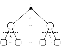
(a) tree-like view

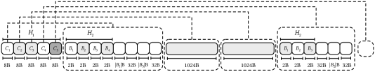
(b) array-like view

Figure 3. The upper part (a) of the picture shows the recursive slicing of the universe $u$ made by the data structure, here viewed as a tree. In the lower part (b), we show how the data structure is concretely laid out in memory, for an example sequence made up of chunks $C_{1}..C_{5}$. In this example, chunks $C_{2}$ and $C_{3}$ are dense, hence represented with bitmaps of 1024 bytes (B); $C_{1}$ and $C_{4}$ are sparse, thus recursively decomposed; lastly, $C_{5}$ is full, hence implicitly represented. Below each box – corresponding to a universe slice – we indicate the number of bytes taken by its encoding. Dashed lines help to graphically translate the array-like view into the tree-like view.

We choose $s_{1}=2^{16}$ and $s_{2}=2^{8}$. Since we consider the case when $u\leq 2^{32}$ and for our choice of $s_{1}=2^{16}$, the number of chunks is always at most $2^{16}$, thus we encode this quantity into 16 bits. Similarly, it follows that each sparse chunk is sliced into at most $2^{8}$ blocks. With this choice of $s_{1}$ and $s_{2}$, a dense chunk is a bitmap of 1024 bytes; a dense block is a bitmap of 32 bytes; a sparse block whose cardinality is $c$ is a sorted array of 8-bit integers, hence taking $c$ bytes overall.

For each non-empty block $[k2^{8},(k+1)2^{8})$, the array $H_{2}$ stores its identifier $k$ and its cardinality. Both quantities are always at most $2^{8}$, thus they take one byte each. Knowing the cardinality $0<c\leq 2^{8}$ of a block we derive the number of bytes needed by its representation. If $c<2^{8}/8-1=31$, the block is considered to be sparse, thus it takes $c$ bytes; otherwise it is dense and takes 32 bytes. Therefore, a sparse block consumes at most $(2^{8}/8-2)\times 8+8=248$ bits. Note that we do not set the sparseness threshold to $2^{8}/8=32$ because otherwise a sparse block would consume at most $256$ bits that is equal to the cost of a dense block and a bitmap would suffice.

For each non-empty chunk $[k2^{16},(k+1)2^{16})$, the array $H_{1}$ stores, instead, the following quantities: its identifier $k$, its cardinality, and the number of bytes needed by its encoding. Similarly to the case of a sparse block, we require the encoding of a sparse chunk to take less than $2^{16}$ bits, otherwise a bitmap of $2^{16}$ bits would suffice. Therefore, each of these 3 quantities easily fits into a 16-bit integer.

Although we could derive the type of a chunk from its cardinality as done for a block, we also store the type explicitly using 16 bits. When a chunk is sparse, we need to know the number of its blocks, i.e., the number of non-empty $2^{8}$-size slices. This number is the size of the corresponding header $H_{2}$. Therefore, we write this quantity in 8 bits and interleaved with the 16 bits dedicated to the type information. In conclusion, we spend a 64-bit overhead per chunk.

Fig. 3b shows an example of such organization and how all the different data quantities (headers, bitmaps and arrays) are laid out in memory. In practice, the logical tree shown in Fig. 3a is “linearized” into an array of bytes.

The data structure described here has similarities with some previous approaches. As already discussed, the universe is exponentially reduced like in a van Emde Boas tree, i.e., $2^{32}\rightarrow 2^{16}\rightarrow 2^{8}$. Partitioning the universe recursively has the potential of adapting to the distribution of the integers being encoded, a crucial design choice for clustered integer sequences such as inverted lists. The choice of bitmaps to represents dense sets is a widely adopted technique, employed by, for example, partitioned Elias-Fano (Ottaviano and Venturini, 2014), hybrid Variable-Byte schemes (Pibiri and Venturini, 2019) and Roaring (Lemire et al., 2018a). However, as we are going to show, the use of bitmaps joint with universe-aligned partitions is particularly effective for fast query execution because operations can be implemented via inexpensive bitwise instructions, hence exploiting word-level parallelism, and are suitable for even more advanced instructions, such as SIMD AVX.

The description above also opens the possibility for better compression. For example, we could use a different representation for sparse blocks, e.g., bit-aligned universal codes. Whatever representation we use, that will give birth to interesting time/space trade-offs. The choice adopted here of $s_{1}=2^{16}$, $s_{2}=2^{8}$ and the use of 8-bit integer arrays clearly favours time efficiency given that both bitmaps and packed arrays are aligned to byte boundaries.

3.2. Operations

We now describe how the operations are supported by the data structure.

Decoding. The $\mathcal{S}$.decode(output) operation decodes $\mathcal{S}$ sequentially to the output buffer of 32-bit integers. We loop through each chunk and, depending on its type, we decode it accordingly appending the result into the output buffer. This permits to write different specialized functions to handle a slice differently based on its type.

Bitmaps can be efficiently decoded using the built-in function ctzll which counts the number of trailing zero into a 64-bit word (Lemire et al., 2018a) (we also tested a SIMD algorithm to decode larger bitmaps but got almost no speed improvement).

The sorted arrays encoding sparse blocks contain at most $2^{8}/8-2$ integers, each value taking 8 bits. Therefore, we can use the SIMD instruction _mm256_cvtepu8_epi32, that zero extend packed (unsigned) 8-bit integers to 32-bit integers. Doing so, we can efficiently decode 8 values at a time. We also observed that this approach is even more efficient when paired with loop unrolling, thus we apply the instruction either 2 or 4 times after a single test on the block cardinality.

Intersection. The operation AND($\mathcal{S}_{1}$, $\mathcal{S}_{2}$, output) performs the intersection between $\mathcal{S}_{1}$ and $\mathcal{S}_{2}$, materializing the result into the output buffer of 32-bit integers and returning the size of the result. We use the algorithm illustrated in Fig. 2b, thus we loop through the header arrays of the sequences, intersecting only chunks/blocks that are shared by the two (line 8). Therefore, we reduce the problem of list intersection to the smaller instance of performing intersections between (1) two bitmaps, or (2) two arrays, or a (3) bitmap and an array (line 9).

Case (1) – the intersection between two bitmaps – translates into a sequence of inexpensive bitwise AND instructions between 64-bit words with (usually) automatic compiler vectorization.

⬇

#define INIT \

__m256i base_v = _mm256_set1_epi32(base); \

__m128i v_l = _mm_lddqu_si128((__m128i const*)l); \

__m128i v_r = _mm_lddqu_si128((__m128i const*)r); \

__m256i converted_v; \

__m128i shuf, p, res; \

int mask, matched;

#define INTERSECT \

res = \

_mm_cmpestrm(v_l, c_l, v_r, c_r, \

_SIDD_UBYTE_OPS | \

_SIDD_CMP_EQUAL_ANY | \

_SIDD_BIT_MASK); \

mask = _mm_extract_epi32(res, 0); \

matched = _mm_popcnt_u32(mask); \

size += matched; \

shuf = _mm_load_si128((__m128i const*)T + mask); \

p = _mm_shuffle_epi8(v_r, shuf); \

converted_v = _mm256_cvtepu8_epi32(p); \

converted_v = _mm256_add_epi32(base_v, converted_v); \

_mm256_storeu_si256((__m256i*)out, converted_v); \

if (matched > 8) { \

p = _mm_bsrli_si128(p, 8); \

converted_v = _mm256_cvtepu8_epi32(p); \

converted_v = _mm256_add_epi32(base_v, converted_v); \

_mm256_storeu_si256((__m256i*)(out + 8), converted_v); \

}

#define ADVANCE(ptr) \

out += size; \

ptr += 16; \

v_##ptr = _mm_lddqu_si128((__m128i const*)ptr); \

c_##ptr -= 16;

Figure 4. C++ macros to support the vectorized implementation of the intersection between small sorted arrays. These macros are used by the code shown in Fig. 5.

Case (2) has to intersect tiny 8-bit sorted arrays. While a scalar textbook intersection algorithm between uncompressed arrays would suffice, we can accelerate the process using a variation of the vectorized approach by Schlegel, Willhalm, and Lehner (2011). In short, the algorithm uses the SIMD instruction _mm_cmpestrm to compare strings of bytes. In our case we can, therefore, execute an all-versus-all comparison in parallel between sets of 16 $\times$ 8-bit integers. Matching integers, i.e., integers in common between the two sets, are marked with a 32-bit bitmap returned as the result of the comparison. We can use this 32-bit value as an index in a pre-computed universal table $T$ of 1024 $\times$ 1024 bytes to obtain a permutation of bytes indexes, indicating how the matching integers should be permuted to collate them to the beginning of a 128-bit register. Such permutation is applied with the dedicated _mm_shuffle_epi8 SIMD instruction. The C++ macro INTERSECT shown in Fig. 4 illustrates this approach. Let $c_{l}$ and $c_{r}$ be the cardinality of the two sets respectively. Since in our case we have that both $c_{l}$ and $c_{r}$ are less than 32, we can directly enumerate the following 3 different cases: (1) $c_{l}\leq 16$ and $c_{r}\leq 16$, then we need only 1 string comparison; (2) $c_{l}\leq 16$ and $c_{r}>16$ (or $c_{r}\leq 16$ and $c_{l}>16$), then we need 2 string comparisons; (3) $c_{l}>16$ and $c_{r}>16$, then we would need 4 string comparisons but we determined that the simple scalar version is more efficient. The C++ function sparse_blocks_and coded in Fig. 5 shows these cases and, along with the code in Fig. 4, completes our intersection algorithm for small sets.

For detailed descriptions of SIMD instructions, refer to the excellent Intel guide at https://software.intel.com/sites/landingpage/IntrinsicsGuide.

⬇

size_t sparse_blocks_and(uint8_t const* l, uint8_t const* r,

int c_l, int c_r,

uint32_t base, uint32_t* out) {

size_t size = 0;

if (c_l <= 16 and c_r <= 16) {

INIT INTERSECT return size; // 1 cmpestr

}

if (c_l <= 16 and c_r > 16) {

INIT INTERSECT ADVANCE(r) INTERSECT return size; // 2 cmpestr

}

if (c_r <= 16 and c_l > 16) {

INIT INTERSECT ADVANCE(l) INTERSECT return size; // 2 cmpestr

}

/* scalar code goes here */

}

Figure 5. The C++ skeleton of the vectorized implementation of the intersection between small sorted arrays. The macros INIT, INTERSECT and ADVANCE are shown in Fig. 4. In the code c_l and c_r indicate the cardinalities of the two arrays respectively; the value base is equal to $k_{1}2^{16}+k_{2}2^{8}$ if we are intersecting the $k_{2}$-th $2^{8}$-long slices of the $k_{1}$-th $2^{16}$-long slice.

Case (3) – the intersection between a bitmap and an array – is implemented by checking if the values of the array correspond to bits set in the bitmap, using the bit-test assembler instruction.

Union. The operation OR($\mathcal{S}_{1}$, $\mathcal{S}_{2}$, output) performs the union between $\mathcal{S}_{1}$ and $\mathcal{S}_{2}$, materializing the result into the output buffer of 32-bit integers and returning the size of the result. The algorithm follows the same skeleton described for the intersection, albeit we do not rely on specific SIMD optimizations: bitmaps are merged using bitwise OR within 64-bit words; sorted arrays using scalar code; the case with a bitmap and an array is handled by first converting the sorted array into a bitmap, then using the parallelism of bitwise OR.

Random access. The operation $\mathcal{S}$.access($i$) returns the integer $\mathcal{S}[i]$. We scan the header array of the data structure to take into account for the cardinality of each chunk covering a universe of size $2^{16}$ in order to locate the chunk containing the $i$-th integer. To make this search faster, we build cumulative cardinality counts for groups of $a$ non-empty universe chunks, thus skipping $a$ chunks if the sum of their cardinalities is less than $i$. The parameter $a$ is an associativity value that in our implementation we set to 32. Then we proceed recursively at the block-level if a chunk is sparse (but we do not build cumulative counts at the block level).

In particular, whenever we encounter a bitmap, we rely on efficiency of the built-in instruction popcountll to locate the 64-bit word where the wanted integer lies in. This instruction returns the number of bits set in a 64-bit word. Now that we have reduced the problem to a word of 64 bits, we can use the parallel-bit deposit assembler instruction pdep to perform a fast select-in-word operation (Pandey et al., 2017).

nextGEQ. The operation $\mathcal{S}$.nextGEQ($x$) returns the integer greater-than or equal-to $x$, that is the smallest integer $z\geq x$. Since our data structure is partitioned by universe, we can directly identify the chunk comprising $z$ because this is the one having identifier $x/2^{16}$, i.e., we consider the 16 most significant bits of the key $x$. The wanted value $z$ lies in such partition or, if $x$ is larger than the maximum value in the partition, it is the minimum (first) value in the partition that follows. Observe that this operation is actually faster than access for universe-aligned methods, because it does not need to search for the wanted partition.

4. Experiments

The aim of this section is twofold: establishing a solid experimental comparison between the two different paradigms described in Section 2 in order to assess the achievable space/time trade-offs and reporting on the effectiveness/efficiency of the Slicing approach introduced in Section 3.

Tested configurations. We compare the configurations summarized in Table 1 for the following reasons. For the paradigm partitioning by cardinality with fixed-sized partitions of 128 integers, we test: Variable-Byte (Thiel and Heaps, 1972) with the SIMD-ized decoding algorithm devised by Plaisance et al. (2015); Interpolative (Moffat and Stuiver, 2000) and Elias-Fano (Ottaviano and Venturini, 2014) as representative of, respectively, highest speed, best compression effectiveness and best space/time trade-off in the literature. As representative of the paradigm partitioning by cardinality with variable-sized partitions, we test the $\epsilon$-optimal Elias-Fano mechanism (Ottaviano and Venturini, 2014). For all such representation, we use the C++ implementation provided in the ds2i library, available at https://github.com/ot/ds2i.

Concerning the paradigm partitioning by universe, we test three solutions. The first two solutions are represented by Roaring (Lemire et al., 2018a) (see Section 2.2). We test the solution without the run-container optimization, thus using two container types (bitmap and sorted array), and with the optimization, thus using three container types (bitmap, sorted array and run). We use the dedicated library written in C and available at https://github.com/RoaringBitmap/CRoaring.

The third solution is the Slicing approach described in Section 3. Our C++ implementation of the mechanism is freely available at https://github.com/jermp/s_indexes.

Method	Shorthand	Strategy
Variable-Byte	V	PC; fixed-sized partitions of 128 integers; byte-aligned
Elias-Fano	EF	PC; fixed-sized partitions of 128 integers; bit-aligned
Interpolative	BIC	PC; fixed-sized partitions of 128 integers; bit-aligned
Elias-Fano $\epsilon$-opt.	PEF	PC; variable-sized partitions; bit-aligned
Roaring without run opt.	R2	PU; single-span; 2 container types; byte-aligned
Roaring with run opt.	R3	PU; single-span; 3 container types; byte-aligned
Slicing	S	PU; multi-span; byte-aligned

Table 1. The different tested configurations.

Datasets. We perform the experiments on the following standard test collections.

• Gov2 is the TREC 2004 Terabyte Track test collection, consisting in roughly 25 million .gov sites crawled in early 2004. The documents are truncated to 256 KB.

• CW09 is the ClueWeb 2009 TREC Category B test collection, consisting in roughly 50 million English web pages crawled between January and February 2009.

• CCNews is a dataset of news freely available from CommonCrawl: http://commoncrawl.org/2016/10/news-dataset-available. Precisely, the datasets consists of the news appeared from 09/01/16 to 30/03/18.

Identifiers were assigned to documents according to the lexicographic order of their URLs (Silvestri, 2007). Table 2 reports the basic statistics for the collections. We choose three different levels of list density $d$, i.e., the ratio between the size of a list and its maximum integer, and compress all lists whose density exceeds $d$. By varying the density, we highlight how compression effectiveness changes for the two different partitioning paradigms used, still focusing on most of the integers in the collections. Refer to Table 3.

Statistic	Gov2	CW09	CCNews
Sequences	$35,636,425$	$92,094,694$	$43,844,574$
Universe	$24,622,347$	$50,131,015$	$43,530,315$
Integers	$5,742,630,292$	$15,857,983,641$	$20,150,335,440$

Table 2. Basic statistics for the test collections.

Density	Statistic	Gov2	CW09	CCNews
$10^{-2}$	Sequences	$3513$	$5802$	$5930$
	Integers	$4,347,653,438$	$11,676,154,022$	$16,677,342,102$
	%	76	74	83
$10^{-3}$	Sequences	$13,276$	$21,924$	$23,085$
	Integers	$5,066,748,826$	$13,864,451,283$	$18,969,946,075$
	%	88	87	94
$10^{-4}$	Sequences	$85,893$	$99,227$	$79,954$
	Integers	$5,390,038,277$	$14,805,194,135$	$19,681,352,639$
	%	94	93	98

Table 3. Dataset statistics for three levels of density. We also indicate the percentage of integers retained from the original collections shown in Table 2.

Experimental setting, methodology and testing details. The experiments are performed on a machine with 4 Intel i7-4790K CPUs clocked at 4.00 GHz, with 32 GB of RAM DDR3 and running Linux 4.13.0. All the code is compiled with gcc 7.2.0 using the highest optimization setting (compilation flags -march=native and -O3).

For the CRoaring library, we compile the code as recommended in the documentation for best performance, i.e., with full support for vectorization. The run-container optimization is enabled by calling the run_optimize function. The implementations of Elias-Fano (both with fixed and variable partitions) and Interpolative do not use explicit vectorization; the implementation of Variable-Byte makes use of the vectorized algorithm devised by Plaisance et al. (2015), called Masked-VByte.

We build the indexes in internal memory and write the corresponding data structure to a file on disk. To perform the queries, the data structure is memory mapped from the file (for CRoaring, by using the frozen_view function) and a warming-up run is executed to fetch the necessary pages from disk.

To sequentially decode the indexes, the kernel is also instructed to access the memory mapped area sequentially using posix_madvice with flag POSIX_MADV_SEQUENTIAL. To test the speed of list queries, namely AND/OR, we generated 1000 random pairs of integers and execute the queries with the corresponding lists. For point queries, namely access and nextGEQ, we similarly execute 1000 random queries for each list of the index. In particular, the 1000 random positions for the access query are not sorted. The input integers for nextGEQ are not sorted either and less then the maximum integer in the sequence (thus, the result is always well determined).

Each run of queries is repeated 10 times to smooth fluctuations during measurements. The time reported is the average among these runs.

Method	$d=10^{-2}$				$d=10^{-3}$				$d=10^{-4}$
	Gov2	CW09	CCNews		Gov2	CW09	CCNews		Gov2	CW09	CCNews
V	$8.598,74$	$8.721,34$	$8.662,18$		$8.716,01$	$9.004,13$	$9.075,28$		$8.848,51$	$9.188,16$	$9.2832$
EF	$2.723,58$	$4.4415$	$4.717,34$		$3.248,97$	$5.144,16$	$5.365$		$3.654,33$	$5.562,65$	$5.655,84$
BIC	$2.331,74$	$3.589,72$	$4.372,32$		$2.721,38$	$4.111,78$	$4.966,99$		$3.016,66$	$4.407,28$	$5.238,47$
PEF	$2.369,12$	$4.008,44$	$4.5165$		$2.846,03$	$4.618,34$	$5.157,98$		$3.200,86$	$4.960,94$	$5.445,76$
R2	$6.003,608$	$8.881,072$	$8.252,430$		$7.027,80$	$9.988,34$	$9.211,68$		$7.601,203$	$10.474,733$	$9.525,385$
R3	$5.331,765$	$8.494,709$	$8.216,347$		$6.245,421$	$9.402,477$	$9.169,742$		$6.745,314$	$9.751,545$	$9.480,298$
S	$3.232,81$	$5.4384$	$5.979,09$		$3.910,38$	$6.390,24$	$7.1822$		$4.455,39$	$7.000,42$	$7.766,09$

Table 4. Space in bits per integer by varying density $d$.

Method	$d=10^{-2}$				$d=10^{-3}$				$d=10^{-4}$
	Gov2	CW09	CCNews		Gov2	CW09	CCNews		Gov2	CW09	CCNews
V	$0.513,518$	$0.606,247$	$0.528,292$		$0.550,443$	$0.662,528$	$0.585,74$		$0.582,142$	$0.706,762$	$0.618,797$
EF	$0.874,415$	$1.286,32$	$1.363,01$		$0.941,314$	$1.341,28$	$1.411,79$		$0.980,144$	$1.357,15$	$1.421,67$
BIC	$5.261,76$	$6.7332$	$7.709,33$		$5.540,49$	$6.948,62$	$7.8628$		$5.7008$	$7.009,13$	$7.901,28$
PEF	$0.784,609$	$1.146,84$	$1.344,22$		$0.857,179$	$1.2216$	$1.480,46$		$0.912,888$	$1.253,57$	$1.5303$
R2	$0.532,040$	$0.716,252$	$0.682,651$		$0.525,104$	$0.697,586$	$0.685,258$		$0.537,158$	$0.706,256$	$0.687,055$
R3	$0.552,781$	$0.755,715$	$0.702,587$		$0.548,563$	$0.760,792$	$0.690,020$		$0.573,709$	$0.776,009$	$0.699,855$
S	$0.563,091$	$0.670,121$	$0.652,603$		$0.571,514$	$0.689,87$	$0.673,231$		$0.598,734$	$0.725,803$	$0.706,615$

Table 5. Average nanoseconds per decoded integer by varying density $d$.

Organization. We organize the experiments in three subsections. At the whole index level (Section 4.1), we are interested in the number of bits spent per represented integer and the time spent per decoded integer when decoding sequentially every list in the index. At the list level (Section 4.2), we report the time needed to compute pair-wise conjunctions (i.e., intersections or boolean AND queries) and pair-wise disjunctions (i.e., unions or boolean OR queries). Finally, at the single integer level (Section 4.3), we evaluate the time needed to decode an integer at a random position and resolve a nextGEQ query.

4.1. Index space and decoding time

Table 4 reports the average number of bits per integer spent by the different methods. Clearly, the bit rate is increasing for decreasing values of density: the sparser a list is, the less clustered it is, thus more bits are needed to represent the values. In general, across all density levels, the bit-aligned methods EF, PEF and BIC offer the best compression effectiveness, with the latter being the most space-efficient of all. Adapting the sizes of the partitions to the distribution of the integers being compressed pays off: PEF is always more effective than EF. The byte-aligned methods V, R2 and R3 are always the largest, with R2 and R3 being always more effective than V on Gov2 but less effective on the other datasets CW09 and CCNews. The use of run containers for the R3 mechanism pays off on the more clustered Gov2, but has a smaller impact on CW09 and CCNews. In general, between the most effective methods and the least effective ones there is a factor of $\approx$2 in space consumption.

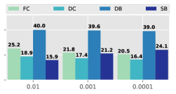
(a) integers ($\%$) – Gov2

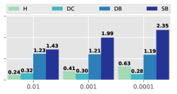
(b) bits per integer – Gov2

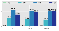
(c) integers ($\%$) – CW09

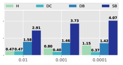
(d) bits per integer – CW09

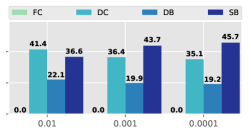
(e) integers ($\%$) – CCNews

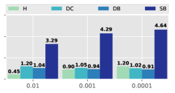
(f) bits per integer – CCNews

Figure 6. Plots (a), (c) and (e) show the percentage of integers covered by the full chunks (FC), dense chunks (DC), dense blocks (DB) and sparse blocks (SB) of the Slicing approach. Plots (b), (d), (f) show, instead, how the bits per integer rate of Slicing is fractioned among headers (H), dense chunks, dense blocks and sparse blocks. For all plots, we show how the breakdowns change by varying density.

Lastly, the S solution stands in a middle position between these two classes, costing roughly $0.9\div 2$ bits per integer more than the most effective methods. In Fig. 6 we report the detailed breakdown of how the integers of the test collections are covered by the different universe slices and how the bits per integer rate is fractioned among them. Not surprisingly, most of the space is spent in the representation of the sparse slices of size $2^{8}$ that roughly cover (an average of) the $20\%$, $37\%$ and $42\%$ of the integers of Gov2, CW09 and CCNews respectively. Another meaningful thing to notice is that more than $20\%$ of the integers of Gov2 are just covered by runs of $2^{16}$ elements and, thus, represented implicitly (dense chunks), whereas this does not happen on the less clustered CW09 and CCNews.

Table 5 reports the average nanoseconds spent per decoded integer, measured by calling the operation decode for each list in the index. The methods V, R2, R3 and S are the fastest. However, V decodes a stream of $d$-gaps and we skipped the final prefix-summing scan in this experiment, whereas R2, R3 and S directly decode the values without the need of further processing (thus, the results compare more favourably for V). There is no appreciable difference between the decoding times of R2 and R3. The other bit-aligned methods EF, PEF and BIC are much slower, with the latter being the least efficient of all. In particular, the ds2i library API does not expose a decode operation, thus we implemented it for Elias-Fano-based methods. In such methods, a partition can be represented using one among three different encodings according to its characteristics, namely its relative universe of representation and size. These encodings include Elias-Fano, a bitmap and an implicit representation whenever the relative universe of a partition is equal to its size (see (Vigna, 2013) and (Ottaviano and Venturini, 2014) for details). Thus, efficient decoding of Elias-Fano codes basically reduces to reading negated unary codes; bitmaps are decoded using the same procedures as used in S (using the built-in ctzll function); implicit partitions are decoded with inexpensive for loops. The sequential decoding speed of Elias-Fano-based methods is, anyway, two times less than the one of the fastest methods.

The BIC mechanism does not feature specific optimizations, except when decoding runs of consecutive integers and is, on average, one order of magnitude slower than the fastest methods.

Method	$d=10^{-2}$				$d=10^{-3}$				$d=10^{-4}$
	Gov2	CW09	CCNews		Gov2	CW09	CCNews		Gov2	CW09	CCNews
V	3648	6671	16954		710	1591	3732		40	214	523
EF	4652	8356	22818		856	1700	4455		40	192	530
BIC	12169	23608	58349		2649	6377	14765		160	905	2323
PEF	4380	7920	21710		826	1640	4185		40	190	490
R2	377	598	1138		99	232	353		10	57	98
R3	503	962	1338		128	331	395		13	75	115
S	507	1080	2370		135	378	820		11	60	159

Table 6. Average microseconds per AND query by varying density $d$.

4.2. List queries: boolean AND/OR

We now consider the two fundamental list-level queries of intersections (boolean AND) and unions (boolean OR). Again, for all methods the result of the query is materialized onto a pre-allocated output buffer of 32-bit integers, thus we slightly modify the ds2i code base to do so (rather than just counting matching integers). To ensure a fair comparison, we also slightly modify the pair-wise intersection and union functions of CRoaring, because these always output a new Roaring data structure resulting from the operation, thus including (potentially expensive) memory allocations during the process. Thus, our modification avoids memory allocation but the result is accumulated in the pre-allocated output buffer mentioned above.

Table 6 shows the result for intersections. The net result is that indexes partitioned by universe, R2, R3 and S, are significantly more efficient than those partitioned by cardinality, thanks to their “simpler” intersection algorithm using substantially less instructions and branches. As discussed, in this context simplicity means that, being aligned to the same relative universe, bitmap intersections can be carried out by a sequence of inexpensive bitwise AND 64-bit operations; sorted array intersections can be accelerated using SIMD-based algorithms. This results in $6\times$ $\div$ $51\times$ faster execution for $d=10^{-2}$; $5\times$ $\div$ $42\times$ for $d=10^{-3}$; $4\times$ $\div$ $23\times$ for $d=10^{-4}$.

As a further evidence of this fact, we report in Table 7 some performance counts collected with the perf Linux utility, when executing the queries on the Gov2 datasets. We choose to report the counts for the PEF method because it is the one generally performing better among the PC solutions. From the numbers reported in the table we can see that both R2 and S perform significantly less instructions and branches, for example, $10\times$ and $8\times$ less instructions for $d=10^{-2}$ and $d=10^{-3}$ respectively, thus confirming our previous claim about the increase of performance. The PEF method is also “data hungry” compared to R2 and S as it is clear from the high number of L1 cache loads. This is explained by the frequent switching of partitions for higher density values. Observe that PEF is actually exploiting the data cache well (for example, only 228$\times 10^{6}$ misses out of 102 $\times 10^{9}$ loads in L1 for $d=10^{-2}$), however, the higher number of L1 references imposes a significant penalty. Also observe that S is generally slower than R2 because of the further slicing into smaller partitions, inducing more branches that are not easily predicted and thus partially eroding the instruction throughput. In fact, the (intentionally) simpler design of R2 is a lot more advantageous for SIMD instructions: to confirm this, we recompiled the CRoaring library by disabling explicit SIMD optimizations and R2 scored the same as S, so vectorization does the difference. However, notice how the difference in efficiency vanishes for lower density values because most of the skipping happens at a coarser level. Furthermore, also observe that the use of run containers in R3 prevents some SIMD optimizations (Lemire et al., 2018a), thus reducing or even annulling the performance gap between R3 and S.

Quantity	$d=10^{-2}$				$d=10^{-3}$				$d=10^{-4}$
	PEF	R2	S		PEF	R2	S		PEF	R2	S
instructions ($\times 10^{9}$)	$440.99$	$41.1$	$40.3$		$79.5$	$9.9$	$10.3$		$3.6$	$1.7$	$0.85$
instructions/cycle	$2.07$	$2.11$	$1.62$		$1.98$	$1.77$	$1.53$		$1.75$	$1.30$	$1.28$
branches ($\times 10^{9}$)	$69.7$	$4.7$	$5.5$		$11.7$	$1.5$	$1.5$		$0.5$	$0.35$	$0.14$
L1 loads ($\times 10^{9}$)	$101.99$	$7.8$	$5.98$		$18.3$	$2.1$	$1.83$		$0.85$	$0.45$	$0.18$
L1 misses ($\times 10^{6}$)	$228.4$	$421.6$	$282.4$		$51.1$	$100.1$	$62.9$		$6.7$	$16.9$	$6.8$
LL loads ($\times 10^{6}$)	$15.7$	$78.2$	$24.4$		$5.45$	$19.8$	$7.8$		$1.49$	$4.1$	$1.85$
LL misses ($\times 10^{6}$)	$11.2$	$35.2$	$14.1$		$4.5$	$12.5$	$5.6$		$1.43$	$3.1$	$1.54$

Table 7. Performance counts collected with the perf Linux utility when executing AND queries on the Gov2 dataset, for the PEF, R2 and S methods, by varying density.

Method	$d=10^{-2}$				$d=10^{-3}$				$d=10^{-4}$
	Gov2	CW09	CCNews		Gov2	CW09	CCNews		Gov2	CW09	CCNews
S with SIMD	507	1080	2370		135	378	820		11	60	159
S without SIMD	816	1959	5190		213	558	1344		13	72	203

Table 8. The performance of the S method when executing AND queries with and without the use of SIMD instructions. Clearly, the first row of the table corresponds to the last row of Table 6.

In Table 8 we also investigate the impact of SIMD instructions for the intersection of small sorted array discussed in Section 3.2. The experiment highlights two important facts, one being the consequence of the other: (1) the vectorization of small arrays pays off, as the results for AND are significantly better with SIMD instructions (roughly $2\times$ better for sufficiently dense sequences); (2) most of the running time is actually spent in intersecting small arrays (not surprisingly, since bitmaps require essentially bitwise instructions that are very cheap). The latter fact explains why the SIMD optimization is so effective and is consistent with the breakdowns reported in Fig. 6. Lastly, the effect of vectorization clearly tends to diminish for smaller sequences, being usually the ones with lower density values, as we can see by comparing the values reported in the columns corresponding to $d=10^{-2}$ and $d=10^{-4}$.

Table 9 shows instead the result for unions. For the same reasons discussed above for intersections, the indexes partitioned by universe are superior. However, due to the scan-based nature of unions, the performance gap with respect to the indexes partitioned by cardinality is not as high as the one for intersections. It is anyway consistent and equal to $4.5\times$ $\div$ $13\times$ for $d=10^{-2}$; $3.7\times$ $\div$ $11.5\times$ for $d=10^{-3}$; $3.6\times$ $\div$ $10.6\times$ for $d=10^{-4}$. Finally, notice that the results for R2, R3 and S are very similar in this case, with R3 being slightly less efficient.

Method	$d=10^{-2}$				$d=10^{-3}$				$d=10^{-4}$
	Gov2	CW09	CCNews		Gov2	CW09	CCNews		Gov2	CW09	CCNews
V	7754	12480	21000		2173	3924	6191		285	920	1407
EF	9540	17952	29600		2704	5495	8589		366	1300	2000
BIC	21115	39190	63972		6369	12898	20408		899	3185	5042
PEF	8900	17000	28349		2560	5230	8300		350	1252	1887
R2	1737	3570	5001		562	1360	1762		80	356	543
R3	1950	4215	5180		638	1657	1812		86	408	551
S	1955	4040	7440		590	1315	2265		73	276	476

Table 9. Average microseconds per OR query by varying density $d$.

4.3. Point queries: access and nextGEQ

For the methods V, EF and BIC, the access($i$) operation returns the integer in position $i$ mod $B$ from the partition of index $\lfloor i/B\rfloor$, for $B=128$ integers in this experimentation. In particular, the V method requires decoding the partition and perform a prefix-summing scan up to position $i$ mod $B$. The PEF method needs to first locate the partition from which to return the integer because partitions have variable sizes. Similarly, all solutions partitioned by universe, R2, R3 and S, have to take into account the cardinality of each chunk covering a universe of size $2^{16}$ in order to locate the chunk containing the $i$-th integer. Table 10 shows the timings of such algorithms.

The EF method provides generally the fastest query time thanks to the constant-time random access algorithm of Elias-Fano, with PEF and S being in close second position. The decoding operation performed by V imposes a performance penalty with respect to such methods, that is more evident for, clearly, sparser datasets. Again, notice that the access time decreases for decreasing values of density, because fewer partitions per encoded sequence are represented. Lastly, S is faster than R2 because the latter adopts a linear search for the proper chunk to access, whereas S builds cumulative cardinality counts. Concerning the R3 variant with run containers, the linear-search approach employed absorbs roughly 90% of the time resulting in a significant slowdown, confirming the experimental conclusions already given by the authors of Roaring (Lemire et al., 2018a).

Table 11 shows instead the results for the nextGEQ($x$) query. In this case, for all methods partitioned by cardinality, the query is resolved by relying on the skip pointers, as explained in Section 2.1. Precisely, the wanted partition is first identified by binary searching $x$ among the skip pointers, then the operation is concluded in the partition. Differently, the mechanism partitioned by universe directly identifies the partition by considering fields of the binary representation of the key $x$. For this reason and as already discussed in Section 3.2, this operation is actually faster than access for universe-aligned methods.

Again, the Elias-Fano-based methods provides generally better efficiency but with R2 and S being faster especially for lower density values: in such cases, S is the fastest thanks to the further skipping introduced within a single partition. The slowdown imposed by the runs in R3 is alleviated by the use of binary search in this case.

Method	$d=10^{-2}$				$d=10^{-3}$				$d=10^{-4}$
	Gov2	CW09	CCNews		Gov2	CW09	CCNews		Gov2	CW09	CCNews
V	195	174	240		155	184	222		105	151	189
EF	118	122	173		88	103	123		58	75	86
BIC	890	835	1295		904	960	1230		685	876	1062
PEF	154	171	210		118	145	126		77	100	72
R2	475	545	610		294	453	402		111	365	310
R3	5604	18710	2852		2151	7681	1221		443	2254	612
S	153	170	244		105	116	152		55	61	78

Table 10. Average nanoseconds per random access query by varying density $d$.

Method	$d=10^{-2}$				$d=10^{-3}$				$d=10^{-4}$
	Gov2	CW09	CCNews		Gov2	CW09	CCNews		Gov2	CW09	CCNews
V	252	226	308		255	226	279		197	181	243
EF	187	122	250		146	155	175		91	113	120
BIC	955	897	1385		951	1012	1290		710	878	1100
PEF	167	182	229		138	157	144		94	118	89
R2	115	137	185		90	119	133		55	80	82
R3	105	138	188		80	115	136		50	72	85
S	145	174	225		90	110	134		48	57	69

Table 11. Average nanoseconds per nextGEQ query by varying density $d$.

5. Conclusions

The problem of introducing a compression format for sorted integer sequences, with good practical intersection/union performance, is old but pervasive in Computer Science, given its many applications, such as web search engines to mention a notable one. Identifying a single solution to the problem is not generally easy, rather the many space/time trade-offs available can satisfy different application requirements and the “best” solution should always be determined by considering the actual data distribution. To this end, we compare the two different paradigms that partition an inverted list for efficient query processing, either by cardinality or by universe.

Figure 7 is a clear summary of such experimental comparison because it shows different space/time trade-off points achievable for the list intersection operation which is the core one for inverted indexes. On the one hand, techniques that use a partitioning-by-cardinality approach offer the best space effectiveness, such as Elias-Fano-based methods and Interpolative; on the other hand, the partitioning-by-universe paradigm offers a remarkably improved intersection efficiency at the expense of space effectiveness, as apparent with the Roaring method. The Slicing solution devised here offers a leading compromise between these two edge points, by combining operational efficiency with space effectiveness. Observe that the Variable-Byte mechanism is generally dominated by other space/time trade-off points: its main strength lies in the simplicity of the implementation and the remarkably compact corresponding code (as far as SIMD instructions are not considered).

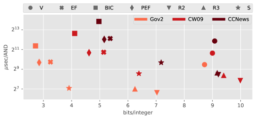
Figure 7. Space/time trade-off curve for the different representations summarized in Table 1, when executing AND queries under a density level of $10^{-3}$. Note the logarithmic scale on the $y$ axis.

Because of the maturity reached by the state-of-the-art and the specificity of the problem, identifying future research directions is not immediate. We mention some promising ones.

In general, devising “simpler” compression formats that can be decoded with algorithms using low-latency instructions (e.g., bitwise) and with as few branches as possible, is a profitable line of research, as demonstrated by the experimentation in this article. Such algorithms favour the super-scalar execution of modern CPUs and are also suitable for SIMD instructions.

Another direction could look at devising dynamic and compressed representations for integer sequences, able of also supporting additions and deletions. This problem is actually a specific case of the more general dictionary problem, which is a fundamental textbook problem. While a theoretical solution already exists with all operations supported in optimal time under succinct space (Pibiri and Venturini, 2017b), an implementation with good practical performance could be of great interest for dynamic inverted indexes.

- (1)
- Anh and Moffat (2005) Vo Ngoc Anh and Alistair Moffat. 2005. Inverted Index Compression Using Word-Aligned Binary Codes. Information Retrieval Journal 8, 1 (2005), 151–166.
- Anh and Moffat (2010) Vo Ngoc Anh and Alistair Moffat. 2010. Index compression using 64-bit words. Software: Practice and Experience 40, 2 (2010), 131–147.
- Broder et al. (2003) Andrei Z. Broder, David Carmel, Michael Herscovici, Aya Soffer, and Jason Y. Zien. 2003. Efficient query evaluation using a two-level retrieval process. In Proceedings of the 12th ACM International Conference on Information and Knowledge Management. 426–434.
- Cambazoglu and Baeza-Yates (2015) B. Barla Cambazoglu and Ricardo Baeza-Yates. 2015. Scalability Challenges in Web Search Engines. Morgan & Claypool Publishers.
- Chambi et al. (2016) Samy Chambi, Daniel Lemire, Owen Kaser, and Robert Godin. 2016. Better bitmap performance with Roaring bitmaps. Software: practice and experience 46, 5 (2016), 709–719.
- Cormen et al. (2009) Thomas H. Cormen, Charles E. Leiserson, Ronald L. Rivest, and Clifford Stein. 2009. Introduction to Algorithms (3rd ed.). MIT Press.
- Dean (2009) Jeffrey Dean. 2009. Challenges in building large-scale information retrieval systems: invited talk. In Proceedings of the 2nd International Conference on Web Search and Data Mining.
- Elias (1974) Peter Elias. 1974. Efficient Storage and Retrieval by Content and Address of Static Files. J. ACM 21, 2 (1974), 246–260.
- Elias (1975) Peter Elias. 1975. Universal codeword sets and representations of the integers. IEEE Transactions on Information Theory 21, 2 (1975), 194–203.
- Fano (1971) Robert Mario Fano. 1971. On the number of bits required to implement an associative memory. Memorandum 61, Computer Structures Group, MIT (1971).
- Golomb (1966) Solomon Golomb. 1966. Run-length encodings. IEEE Transactions on Information Theory 12, 3 (1966), 399–401.
- Lemire and Boytsov (2015) Daniel Lemire and Leonid Boytsov. 2015. Decoding billions of integers per second through vectorization. 45, 1 (2015), 1–29.
- Lemire et al. (2018a) Daniel Lemire, Owen Kaser, Nathan Kurz, Luca Deri, Chris O’Hara, François Saint-Jacques, and Gregory Ssi-Yan-Kai. 2018a. Roaring bitmaps: Implementation of an optimized software library. Software: Practice and Experience 48, 4 (2018), 867–895.
- Lemire et al. (2018b) Daniel Lemire, Nathan Kurz, and Christoph Rupp. 2018b. Stream-VByte: faster byte-oriented integer compression. Inform. Process. Lett. 130 (2018), 1–6.
- Lemire et al. (2016) Daniel Lemire, Gregory Ssi-Yan-Kai, and Owen Kaser. 2016. Consistently faster and smaller compressed bitmaps with roaring. Software: Practice and Experience 46, 11 (2016), 1547–1569.
- Mallia et al. (2017) Antonio Mallia, Giuseppe Ottaviano, Elia Porciani, Nicola Tonellotto, and Rossano Venturini. 2017. Faster BlockMax WAND with Variable-sized Blocks. In Proceedings of the International ACM Conference on Research and Development in Information Retrieval. 625–634.
- Manning et al. (2008) Christopher Manning, Prabhakar Raghavan, and Hinrich Schütze. 2008. Introduction to Information Retrieval. Cambridge University Press.
- Moffat (2008) Alistair Moffat. 2008. Compressing integer sequences and sets. In Encyclopedia of algorithms. Springer, 1–99.
- Moffat and Petri (2017) Alistair Moffat and Matthias Petri. 2017. ANS-Based Index Compression. In Proceedings of the ACM on Conference on Information and Knowledge Management. 677–686.
- Moffat and Petri (2018) Alistair Moffat and Matthias Petri. 2018. Index Compression Using Byte-Aligned ANS Coding and Two-Dimensional Contexts. In Proceedings of the 11th ACM International Conference on Web Search and Data Mining. 405–413.
- Moffat and Stuiver (1996) Alistair Moffat and Lang Stuiver. 1996. Exploiting Clustering in Inverted File Compression. In Data Compression Conference. 82–91.
- Moffat and Stuiver (2000) Alistair Moffat and Lang Stuiver. 2000. Binary Interpolative Coding for Effective Index Compression. Information Retrieval Journal 3, 1 (2000), 25–47.
- Ottaviano and Venturini (2014) Giuseppe Ottaviano and Rossano Venturini. 2014. Partitioned Elias-Fano Indexes. In Proceedings of the 37th International Conference on Research and Development in Information Retrieval. 273–282.
- Pandey et al. (2017) Prashant Pandey, Michael A Bender, and Rob Johnson. 2017. A fast x86 implementation of select. arXiv preprint arXiv:1706.00990 (2017).
- Pibiri et al. (2019) Giulio Ermanno Pibiri, Matthias Petri, and Alistair Moffat. 2019. Fast Dictionary-Based Compression for Inverted Indexes. In International ACM Conference on Web Search and Data Mining. 9.
- Pibiri and Venturini (2017a) Giulio Ermanno Pibiri and Rossano Venturini. 2017a. Clustered Elias-Fano indexes. ACM Transactions on Information Systems 36, 1, Article 2 (2017), 33 pages.
- Pibiri and Venturini (2017b) Giulio Ermanno Pibiri and Rossano Venturini. 2017b. Dynamic Elias-Fano Representation. In Proceedings of the 28-th Annual Symposium on Combinatorial Pattern Matching. 30:1–30:14.
- Pibiri and Venturini (2018) Giulio Ermanno Pibiri and Rossano Venturini. 2018. Inverted Index Compression. Encyclopedia of Big Data Technologies (2018), 1–8.
- Pibiri and Venturini (2019) Giulio Ermanno Pibiri and Rossano Venturini. 2019. On Optimally Partitioning Variable-Byte Codes. IEEE Transactions on Knowledge and Data Engineering (2019), 1–12.
- Plaisance et al. (2015) Jeff Plaisance, Nathan Kurz, and Daniel Lemire. 2015. Vectorized VByte Decoding. In International Symposium on Web Algorithms.
- Robertson and Jones (1976) Stephen Robertson and Sparck Jones. 1976. Relevance weighting of search terms. Journal of the American Society for Information Science 27, 3 (1976), 129–146.
- Schlegel et al. (2011) Benjamin Schlegel, Thomas Willhalm, and Wolfgang Lehner. 2011. Fast Sorted-Set Intersection using SIMD Instructions.. In ADMS@ VLDB. 1–8.
- Scholer et al. (2002) Falk Scholer, Hugh E Williams, John Yiannis, and Justin Zobel. 2002. Compression of inverted indexes for fast query evaluation. In Proceedings of the 25th annual international ACM SIGIR conference on Research and development in information retrieval. ACM, 222–229.
- Silvestri (2007) Fabrizio Silvestri. 2007. Sorting Out the Document Identifier Assignment Problem. In Proceedings of the 29th European Conference on IR Research. 101–112.
- Stepanov et al. (2011) Alexander Stepanov, Anil Gangolli, Daniel Rose, Ryan Ernst, and Paramjit Oberoi. 2011. SIMD-based decoding of posting lists. In Proceedings of the 20th International Conference on Information and Knowledge Management. 317–326.
- Thiel and Heaps (1972) Larry H Thiel and HS Heaps. 1972. Program design for retrospective searches on large data bases. Information Storage and Retrieval 8, 1 (1972), 1–20.
- Trotman (2014) Andrew Trotman. 2014. Compression, SIMD, and postings lists. In Proceedings of the 2014 Australasian Document Computing Symposium. ACM, 50.
- van Emde Boas (1975) Peter van Emde Boas. 1975. Preserving Order in a Forest in less than Logarithmic Time. In Proceedings of the 16-th Annual Symposium on Foundations of Computer Science. 75–84.
- van Emde Boas (1977) Peter van Emde Boas. 1977. Preserving Order in a Forest in Less Than Logarithmic Time and Linear Space. Inform. Process. Lett. 6, 3 (1977), 80–82.
- Vigna (2013) Sebastiano Vigna. 2013. Quasi-succinct indices. In Proceedings of the 6th ACM International Conference on Web Search and Data Mining. 83–92.
- Wang et al. (2017) Jianguo Wang, Chunbin Lin, Yannis Papakonstantinou, and Steven Swanson. 2017. An experimental study of bitmap compression vs. inverted list compression. In Proceedings of the 2017 ACM International Conference on Management of Data. ACM, 993–1008.
- Witten et al. (1999) Ian Witten, Alistair Moffat, and Timothy Bell. 1999. Managing gigabytes: compressing and indexing documents and images (2nd ed.). Morgan Kaufmann.
- Yan et al. (2009) Hao Yan, Shuai Ding, and Torsten Suel. 2009. Inverted index compression and query processing with optimized document ordering. In Proceedings of the 18th International Conference on World Wide Web. 401–410.
- Zhang et al. (2008) J. Zhang, X. Long, and T. Suel. 2008. Performance of compressed inverted list caching in search engines. In International World Wide Web Conference (WWW). 387–396.
- Zobel and Moffat (2006) Justin Zobel and Alistair Moffat. 2006. Inverted files for text search engines. Comput. Surveys 38, 2 (2006), 1–56.
- Zukowski et al. (2006) Marcin Zukowski, Sándor Héman, Niels Nes, and Peter Boncz. 2006. Super-Scalar RAM-CPU Cache Compression. In Proceedings of the 22nd International Conference on Data Engineering. 59–70.