Kinematic Constraints on Spatial Curvature from Supernovae Ia and Cosmic Chronometers
Abstract
An approach to estimate the spatial curvature from data independently of dynamical models is suggested, through kinematic parameterizations of the comoving distance () with third degree polynomial, of the Hubble parameter () with a second degree polynomial and of the deceleration parameter () with first order polynomial. All these parameterizations were done as function of redshift . We used SNe Ia dataset from Pantheon compilation with 1048 distance moduli estimated in the range with systematic and statistical errors and a compilation of 31 data estimated from cosmic chronometers. The spatial curvature found for parametrization was . The parametrization for deceleration parameter resulted in . The parametrization has shown incompatibilities between and SNe Ia data constraints, so these analyses were not combined. The and parametrizations are compatible with the spatially flat Universe as predicted by many inflation models and data from CMB. This type of analysis is very appealing as it avoids any bias because it does not depend on assumptions about the matter content of the Universe for estimating .
keywords:
Spatial Curvature – Redshift – Polynomial Parameterization1 Introduction
The evidence that the universe is accelerated first came from Supernovae Ia (SNe Ia) observations (Riess et al., 1998; Perlmutter et al., 1999; Astier et al., 2006; Riess et al., 2007; Davis et al., 2007; Kowalski et al., 2008; Amanullah et al., 2010; Suzuki et al., 2012) and was subsequently complemented by data from Cosmic Microwave Background (CMB) radiation (Komatsu et al., 2011; Larson et al., 2011; Planck Collaboration et al., 2014), Baryonic Acoustic Oscillations (BAO) (Eisenstein et al., 2005; Percival et al., 2007; Schlegel et al., 2009; Eisenstein et al., 2011; Dawson et al., 2013), and the Hubble parameter data (Farooq et al., 2013; Farooq & Ratra, 2013; Farooq et al., 2017). The acceleration phase of the universe can be supported by a simple theoretical model using the cosmological constant plus Cold Dark Matter component (Davis et al., 1985; Bertone & Silk, 2010; Weinberg et al., 2013). This model has cosmological parameters that have been restricted more and more, and have become very precise by observational data (Planck Collaboration et al., 2014; Farooq & Ratra, 2013; Sharov & Vorontsova, 2014).
In addition to the “standard” model that emerges from in the context of Cold Dark Matter, other models have been proposed to explain the problem of accelerated expansion of the universe. Many of these models have as their main idea, a dark energy fluid that produces a negative pressure that would fill the universe (Peebles & Ratra, 2003; Sahni & Starobinsky, 2006). Many hypotheses suggest the nature of this unknown fluid as scalar fields and quintessential models (Amendola, 2000; Sahni & Wang, 2000; Chiba et al., 2000; Capozziello & Fang, 2002; Khurshudyan et al., 2014). Other approaches dealing with accelerated expansion come from modified gravity theories (Volkov, 2012), and , with and being the Ricci and Energy-Momentum trace scalars (Moraes, 2019; Harko et al., 2011), respectively, which generalize the general theory of relativity (Sotiriou & Faraoni, 2010; Guo & Frolov, 2013; Capozziello & de Laurentis, 2011), are also investigated; models based on extra dimensions: as models of the braneworld (Randall & Sundrum, 1999; Falkowski et al., 2000; Binetruy & Langlois, 2000; Shiromizu et al., 2000; Cline et al., 1999), strings (Damour & Polyakov, 1994) and Kaluza-Klein (Overduin & Wesson, 1997), among other works. Having adopted a specific model, cosmological parameters can be determined based on statistical analysis of observational data. All of these suggested hypotheses need first of all to be sifted through observational data. This is the way to study cosmology in the present times.
On the other hand, some works attempt to investigate the history of the universe independently of dynamical models. These approaches are called cosmography models or cosmokinetic models (Visser, 2004, 2005; Shapiro & Turner, 2006; Blandford et al., 2005; Elgarøy & Multamäki, 2006a; Rapetti et al., 2007). The work of (Capozziello et al., 2020) suggests comparing two different parameterizations: auxiliary variables versus Padé polynomials for high redshifts. Both approaches are made in the context of cosmography, where the scale parameter is expanded on Taylor series at the present time . This work compares both analysis through the AIC (Akaike Information Criterion) and the BIC (Bayesian Information Criterion) and showed that the parameterization from the Padé expansion was more promising in the estimate of , and .
In this paper, we will refer to them only as kinematic models, whose name comes from the idea that the universe expansion (or its kinematics) is described by the Hubble expansion rate , deceleration parameter and the jerk parameter , where is the Friedmann-Lemaître-Robertson-Walker (FLRW) metric scale factor. That is, this approach relies only on the Cosmological Principle, which states that the Universe is statistically homogeneous and isotropic at large scales. Assuming an FLRW metric, which is exactly homogeneous and isotropic, one then looks for hints of evolution directly from data. In this parameterization, dark matter dominated the universe, while the CDM accelerated model has . These analyses allow us to study the transition from decelerated to accelerated phases, while the parameter allows you to study deviations from the cosmic concordance model without the restriction of a specific model.
There are several works in the literature that estimated cosmological parameters independently of energy content, in which some authors used parameterization in these estimates (Mortsell & Jonsson, 2011; Yu & Wang, 2016). In (Sapone et al., 2014), an expansion of the comoving distance was made, as a function of , while (L’Huillier & Shafieloo, 2017) reconstructed the luminosity distance with a lognormal kernel using data from BAO and SNeIa (BOSS DROSS 12 and JLA). Furthermore, in (Wei & Wu, 2017) the distance modulus was reconstructed from data using Gaussian processes and compared with from SNe Ia to estimate . In (Heavens et al., 2014), is estimated from BAO data regardless of the model. Other parameters were used by (Montanari & Räsänen, 2017) to analyse the consistency conditions of FRW. And other authors, such as (Collett et al., 2019) and (Liao et al., 2019) estimated the values of and from gravity lensing data and SNe Ia data where the latter used Gaussian Processes (GP).
All these parametrizations help to reconstruct the Universe evolution without mentioning the dynamics, that is, without the use of Einstein’s Equations. Furthermore, by using the FLRW metric geometry, we may relate these parametrizations (, ) to spatial curvature and cosmological distances: luminosity-distance () and angular diameter distance (). So, by using distance data, like the ones provided by SNe Ia, one may constrain spatial curvature, without assuming any particular Cosmology dynamics. This was first shown by (Clarkson et al., 2008).
A first test of this method was done by Mörtsell and Clarkson (Mörtsell & Clarkson, 2009). By using only SNe Ia data and 3 parametrizations of , namely, constant, piecewise and linear on , they have shown that the Universe is currently accelerating regardless of spatial curvature, but could not conclude about an early expansion deceleration. By combining SNe Ia data with BAO, they concluded that the Universe could have early deceleration only for a flat or open Universe (). It has been shown that future 21 cm intensity experiments can improve model-independent determinations of the spatial curvature (Witzemann et al., 2018).
(Yu et al., 2018) have compiled 36 data of , where 31 are measured by using the chronometric technique, while 5 come from BAO (Baryon Acoustic Oscillations) observations. This work used Gaussian Processes (GP) to estimate the continuous function of with values of , and to test the CDM model. They have found . Using the profile of function they estimate limits for the curvature parameter . It was found that the transition from deceleration to acceleration redshift is to of significance and the value of , which is consistent with a spatially flat universe. (Di Valentino et al., 2020) argue that there is a crisis in Cosmology due to interval values of obtained from Planck Legacy 2018 (PL2018), , incompatible with a spatially flat Universe, at more than 99% c.l.
In the present work we study the spatial curvature by means of a third order parametrization of the comoving distance, a second order parametrization of and a linear parametrization of . By combining luminosity distances from SNe Ia (Scolnic et al., 2018) and measurements (Magaña et al., 2018), it is possible to determine values in these cosmological models, independently of the matter content of the Universe. In this type of approach, we obtain an interesting complementarity between the observational data and, consequently, tighter constraints on the parameter spaces.
2 Basic equations
For general cosmologies, the spatial curvature could not be constrained from a simple parametrization of the cosmological observables. However, as curvature relates to geometry, if one parametrizes the dynamics, the geometry can be constrained through the relation among distances and dynamic observables. To realize this, let us assume as a premise the validity of the Cosmological Principle, which leads us to the Friedmann-Lemaître-Robertson-Walker metric:
| (1) |
In the context of the FLRW metric, the line-of-sight distance distance can be estimated. This is the distance between two objects in the universe that remain constant if the objects are moving with the Hubble flow (Hogg, 1999). The line-of-sight comoving distance between an object in redshift and us is given by
| (2) |
where is the Hubble distance and the dimensionless Hubble parameter . As all cosmological distances scale with , we shall adopt the notation where a distance written in upper case () is dimensionless, while a distance written in lower case () is dimensionful and . So, we may write
| (3) |
From this we may obtain the transverse comoving distance. The comoving distance between two events at the same redshift but separated on the sky by some angle is and the transverse comoving distance is related to the line-of-sight comoving distance as:
| (4) |
where we have used the curvature parameter density . By defining the following function
| (5) |
Eq. (4) can be simplified as
| (6) |
The luminosity distance is defined by the relationship between bolometric flux and bolometric luminosity :
| (7) |
We may relate it to the transverse comoving distance by
| (8) |
We shall briefly mention the dynamics here just to show how the curvature density parameter definition emerges. As it is well known, the Friedmann equations can be written as:
| (9) | |||||
| (10) |
where represents the total energy density and the total pressure. As it can be seen, the spatial curvature contributes to the Hubble parameter through Eq. (9), while it does not contribute to acceleration () explicitly (10). The Friedmann equation shows that if we know the matter-energy content of the Universe, we can estimate its spatial curvature. This can be clearly seen if we rewrite Eq. (9) as
| (11) |
where is the total energy density parameter and is the curvature parameter.
Here, we intend to obtain constraints over spatial curvature without making any assumptions about the matter-energy content of the Universe. Thus, we shall assume kinematic expressions for the observables like , and .
Assuming this kinematic approach, we can see that data alone cannot constrain spatial curvature, but luminosity distances from SNe Ia can constrain it through the dependence in Eq. (4). Concerning the deceleration parameter , it can be given as
| (12) |
So, as expected from Eq. (10), a kinematical parametrization will not depend explicitly on spatial curvature, however, the spatial curvature can be constrained through the distance relation (4).
Therefore, we may access the value of through a parametrization of both and . As a third method we can also parametrize the line-of-sight comoving distance, which is directly related to the luminosity distance, in order to obtain the spatial curvature. In what follows we present the three different methods considered here.
2.1 Choice of parametric functions for , and
We shall perform a model selection in order to find the ideal polynomial that better describes the data for the , and parametrizations. The best Bayesian tool for model selection is Bayesian Evidence (Kass & Raftery, 1995; Elgarøy & Multamäki, 2006b; Guimarães et al., 2009; Jesus et al., 2017). However, the Bayesian Evidence, in general, is given by multidimensional integrals over the parameters, so it is usually hard to evaluate. A way around this difficulty is by using its approximation, first obtained by Schwarz (Schwarz, 1978; Liddle, 2004), known as BIC. Bayesian Information Criterion (BIC) (Valentim et al., 2011b, a; Szydłowski et al., 2015) heavily penalizes models with different number of free parameters.
Here we use BIC (Bayesian Information Criterion) in order to find the ideal polynomial order in each of the parametrizations aiming to find model-independent constraints on spatial curvature. The BIC is given by:
| (13) |
where is the number of free parameters and is the number of data. As the likelihood is given by
| (14) |
then, we may write
| (15) |
The interpretation of BIC outcomes is described in Table 1.
| Support | |
|---|---|
| No worth more than a bare mention | |
| Significant/Weak | |
| Strong to very strong/Significant | |
| Decisive/Strong |
The results for the three parametrizations can be seen on Table 2.
| Parametrization | Polynomial order | BIC | BIC | ||
|---|---|---|---|---|---|
| 1 | 1250.825 | 1.16140 | 1264.793 | +193.915 | |
| 2 | 1049.927 | 0.97577 | 1070.878 | 0 | |
| 3 | 1043.839 | 0.97101 | 1071.775 | +0.897 | |
| 4 | 1042.471 | 0.97064 | 1077.390 | +6.512 | |
| 1 | 1059.386 | 0.98456 | 1080.338 | +9.253 | |
| 2 | 1043.150 | 0.97037 | 1071.085 | 0 | |
| 3 | 1042.975 | 0.97111 | 1077.894 | +6.809 | |
| 0 | 1066.636 | 0.99130 | 1087.588 | +16.036 | |
| 1 | 1043.617 | 0.97081 | 1071.552 | 0 | |
| 2 | 1042.919 | 0.97106 | 1077.838 | +6.286 | |
| 3 | 1042.375 | 0.97146 | 1084.278 | +12.726 |
As can be seen on Table 2, the ideal polynomial order for , and are 2, 2 and 1, respectively. However, for , the third degree polynomial can not be discarded by this analysis (). We have tested the second degree parametrization for and have found a too close Universe ( at 68% c.l.), which was in disagreement with the parametrizations and with other data, like CMB (Planck Collaboration et al., 2018). As the third order parametrization can not be discarded by this analysis, we chose to work with this order for .
2.2 from line-of-sight comoving distance,
In order to put limits on by considering the line-of-sight comoving distance, we can write as a third degree polynomial such as:
| (16) |
where and are free parameters. From Eq.(2), we may write
| (17) |
2.3 from
In order to assess by means of we need an expression for . If one wants to avoid dynamical assumptions, one must resort to kinematical methods which use an expansion of over the redshift.
Let us try a simple expansion, namely, the quadratic expansion:
| (20) |
In order to constrain the model with SNe Ia data, we obtain the luminosity distance from Eqs.(8), (3) and (20). We have
| (21) |
which gives three possible solutions, according to the sign of , such as
| (25) |
from which follows the luminosity distance .
2.4 from
Now we can analyze by parametrizing . From (12) one may find as
| (26) |
If we assume a linear dependence in , as
| (27) |
which is the simplest parametrization that allows for an acceleration transition as required by SNe Ia data (Riess et al., 2004; Lima et al., 2012), one may find
| (28) |
while the line-of-sight comoving distance (3) is given by
| (29) |
where is the incomplete gamma function defined in (Abramowitz et al., 1988) as , with , from which follows the luminosity distance as , which can be constrained from observational data.
3 Samples
3.1 dataset
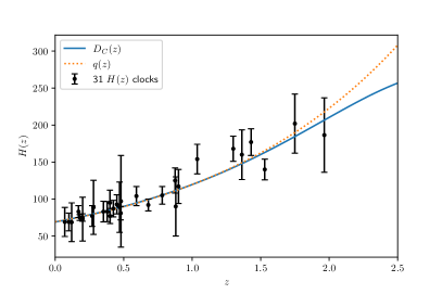
In order to constrain the free parameters, we use the Hubble parameter () data in different redshift values. These kind of observational data are quite reliable because in general such observational data are independent of the background cosmological model, just relying on astrophysical assumptions. We have used the currently most complete compilation of data, with 51 measurements (Magaña et al., 2018).
At the present time, the most important methods for obtaining data are111See (Lima et al., 2012) for a review. (i) through “cosmic chronometers”, for example, the differential age of galaxies (DAG) (Simon et al., 2005; Stern et al., 2010; Moresco et al., 2012; Zhang et al., 2014; Moresco, 2015; Moresco et al., 2016), (ii) measurements of peaks of acoustic oscillations of baryons (BAO) (Gaztañaga et al., 2009; Blake et al., 2012; Busca et al., 2013; Anderson et al., 2014; Font-Ribera et al., 2014; Delubac et al., 2015) and (iii) through correlation function of luminous red galaxies (LRG) (Chuang & Wang, 2013; Oka et al., 2014).
Among these methods for estimating , the 51 data compilation as grouped by (Magaña et al., 2018), consists of 20 clustering (BAO+LRG) and 31 differential age data.
Differently from (Magaña et al., 2018), we choose not to use in our main results here, due to the current tension among values estimated from different observations (Riess et al., 2016; Planck Collaboration et al., 2016; Bernal et al., 2016).
The method used to estimate data from BAO depends on the choice of a fiducial cosmological model. Even if it has an weak model dependence, we choose here not to work with the data from BAO. So, in order to keep the analysis the most model-independent possible, we shall work here only with the 31 differential age data (cosmic chronometers) from (Magaña et al., 2018).
3.2 SNe Ia
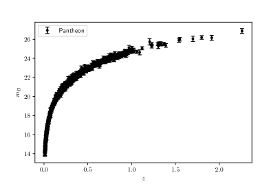
We have chosen to work with one of the largest SNe Ia sample to date, namely, the Pantheon sample (Scolnic et al., 2018). This sample consists of 279 SNe Ia from Pan-STARRS1 (PS1) Medium Deep Survey (), combined with distance estimates of SNe Ia from Sloan Digital Sky Survey (SDSS), SNLS and various low- and Hubble Space Telescope samples to form the largest combined sample of SNe Ia, consisting of a total of 1048 SNe Ia in the range of .
As explained on (Scolnic et al., 2018), the PS1 light-curve fitting has been made with SALT2 (Guy et al., 2010), as it has been trained on the JLA sample (Betoule et al., 2014). Three quantities are determined in the light-curve fit that are needed to derive a distance: the colour , the light-curve shape parameter and the log of the overall flux normalization . We can see the data for Pantheon at Fig. 1a.
The SALT2 light-curve fit parameters are transformed into distances using a modified version of the Tripp formula (Tripp & Branch, 1999),
| (30) |
where is the distance modulus, is a distance correction term based on the host galaxy mass of the SN, and is a distance correction factor based on predicted biases from simulations. As can be seen, is the coefficient of the relation between luminosity and stretch, while is the coefficient of the relation between luminosity and color, and is the absolute -band magnitude of a fiducial SN Ia with and .
Differently from previous SNe Ia samples, like JLA (Betoule et al., 2014), Pantheon uses a calibration method named BEAMS with Bias Corrections (BBC), which uses cosmological simulations assuming a reference CDM model. The cosmological dependence is expected to be small, so neglecting this dependence, allows one to determine SNe Ia distances without one having to fit SNe parameters jointly with cosmological parameters. Thus, Pantheon provide directly corrected estimates in order for one to constrain cosmological parameters alone.
The systematic uncertainties were propagated through a systematic uncertainty matrix. An uncertainty matrix C was defined such that
| (31) |
The statistical matrix has only a diagonal component that includes photometric errors of the SN distance, the distance uncertainty from the mass step correction, the uncertainty from the distance bias correction, the uncertainty from the peculiar velocity uncertainty and redshift measurement uncertainty in quadrature, the uncertainty from stochastic gravitational lensing, and the intrinsic scatter.
4 Analyses and Results
In our analyses, we have chosen flat priors for all parameters, so always the posterior distributions are proportional to the likelihoods.
For data, the likelihood distribution function is given by ,
with
| (32) |
The function for Pantheon is given by
| (33) |
where C is the same from (31), , and
| (34) |
where is a nuisance parameter which encompasses and . We choose to project over , which is equivalent to marginalize the likelihood over , up to a normalization constant. In this case we find the projected :
| (35) |
where , , and .

In order to obtain the constraints over the free parameters, the likelihood , where , has been sampled through a Monte Carlo Markov Chain (MCMC) analysis. A simple and powerful MCMC method is the so called Affine Invariant MCMC Ensemble Sampler by (Goodman & Weare, 2010), which was implemented in Python language with the emcee software by (Foreman-Mackey et al., 2013).
We used the free software emcee to sample from our likelihood in -dimensional parameter space. In order to plot all the constraints on each model in the same figure, we have used the freely available software getdist222getdist is part of the great MCMC sampler and CMB power spectrum solver COSMOMC, by (Lewis & Bridle, 2002)., in its Python version. The results of our statistical analyses can be seen on Figs. 2-7 and on Table 3.
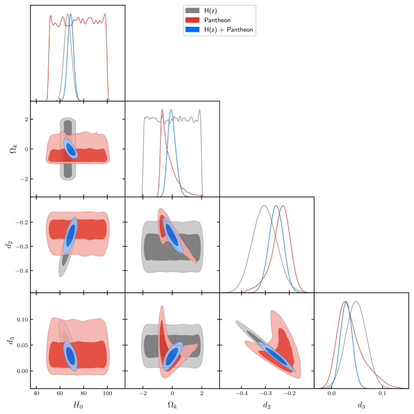
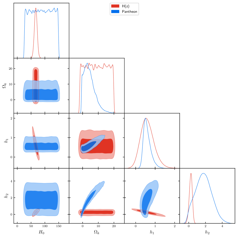
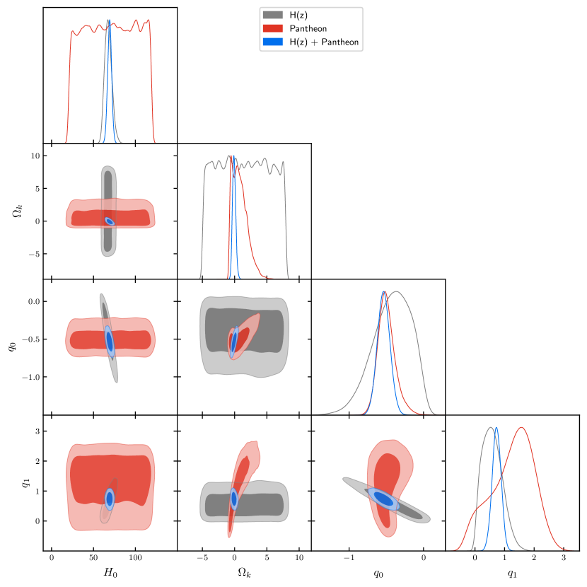
In Figs. 2-4, we show explicitly the independent constraints, in order to see the complementarity between SNe Ia and data. First of all, as expected, SNe Ia does not constrain . In SNe confidence level contours, is only limited by our prior, but data gives good constraints over . We can see also, that in general, SNe Ia alone does not constrain well , but by combining with , which constrain the other parameters, good constraints over the curvature are found. In the planes not containing (, and ) we can see that also helps to reduce a lot the allowed parameter space.
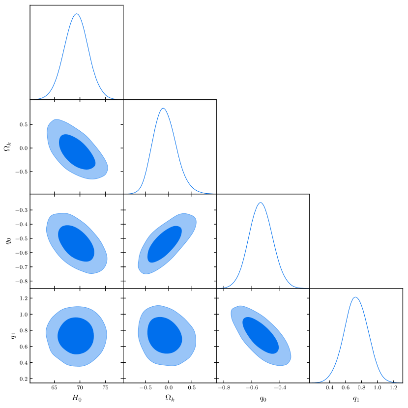
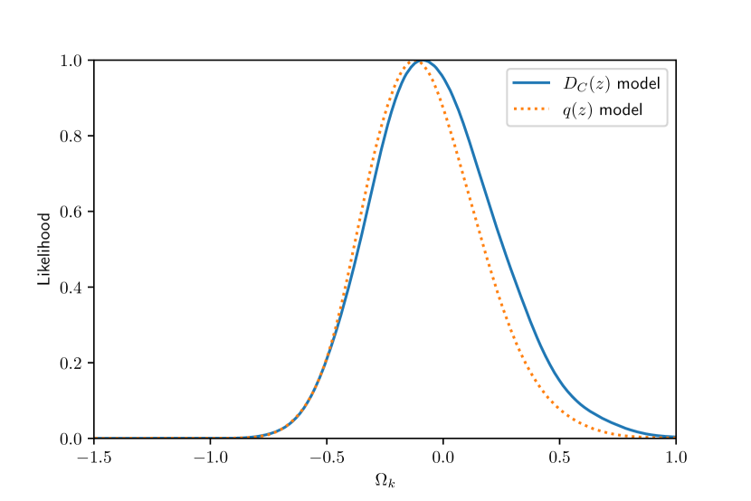
In Figs. 5-6, we have the combined results for each parameterization, where we can clearly see how the combination SNe Ia+ yields good constraints over , as well as the other kinematic parameters. For all parametrizations, the best constraints over the spatial curvature comes from model, as can be seen on Fig. 7. We can also see in this Figure that all constraints are compatible at 1 c.l. Finally, Table 3 shows the full numerical results from our statistical analysis.
| Parameter | ||
|---|---|---|
| – | ||
| – | ||
| – | ||
| – |
Comparing with previous results in the literature, Li et al. (2016) have combined 22 data from cosmic chronometers with Union 2.1 SNe Ia data and JLA SNe Ia data. The combination with Union 2.1 yielded and they found from JLA combination. Wang et al. (2017) have put model independent constraints over and opacity from JLA SNe Ia data and 30 data. They have used Gaussian Processes method and have obtained , with a high uncertainty, due to degeneracy with opacity. It is worth to mention that, although model-independent, both (Li et al., 2016) and (Wang et al., 2017) have followed a different approach from the present paper. They do not parametrize any cosmological observable, instead they obtain a distance modulus from data, and compare with distance modulus from SNe Ia, which are dependent on spatial curvature. As already mentioned, Yu et al. (2018) have used and BAO, with the aid of Gaussian Processes and have found , consistent with our results. By combining CMB data with BAO, in the context of CDM, the Planck Collaboration et al. (2018) have found . It is consistent with our result, but it is dependent on the chosen dynamical model, CDM.
Another interesting result that can be seen on Table 3 is the constraint. As one may see, the constraints over are consistent among both parametrizations. The constraints over are quite stringent today from many observations (Riess et al., 2019; Planck Collaboration et al., 2018). However, there is some tension among values estimated from Cepheids (Riess et al., 2019) and from CMB (Planck Collaboration et al., 2018). While Riess et al. advocate km/s/Mpc, the Planck collaboration analysis, in the context of CDM, yields km/s/Mpc, a 4.4 lower value.
It is interesting to note, from our Table 3 that, although we are working with model independent parametrizations and data at intermediate redshifts, our result is in better agreement with the high redshift result from Planck. In fact, all our results are compatible within 1 with the Planck’s result, while, for the Riess’ result, our result is marginally compatible at 1.8, and is marginally compatible at 1.7.
5 Conclusion
In the present work, we wrote the comoving distance , the Hubble parameter and the deceleration parameter as third, second and first degree polynomials on , respectively (see equations (16), (20) and (27)), and obtained, for each case, the value. We have shown that by combining Supernovae type Ia data and Hubble parameter measurements, nice constraints are found over the spatial curvature, without the need of assuming any particular dynamical model. Our results can be found in Figures 2-6. As one may see from Figs. 2-4, the analyses by using SNe Ia and data are complementary to each other, providing tight limits in the parameter spaces. As a result, the values obtained for the spatial curvature in each case were and at 1 c.l., for and parametrizations (see Fig. 7), all compatible with a spatially flat Universe, as predicted by most inflation models and confirmed by CMB data, in the context of CDM model. The parametrization presented incompatibilities from its constraints coming from SNe Ia and cosmic clocks data and was not considered in the joint analysis.
Further investigations could include different parametrizations and other kinematical methods in order to determine the Universe spatial curvature independently from the matter-energy content.
6 Acknowledgements
JFJ is supported by Fundação de Amparo à Pesquisa do Estado de São Paulo - FAPESP (Process no. 2017/05859-0). RV and MM are supported by Fundação de Amparo à Pesquisa do Estado de São Paulo - FAPESP (thematic project process no. 2013/26258-2 and regular project process no. 2016/09831-0). MM is also supported by CNPq and Capes. PHRSM also thanks CAPES for financial support.
Data Availability
No new data were generated or analysed in support of this research.
References
- Abramowitz et al. (1988) Abramowitz M., Stegun I. A., Romer R. H., 1988, American Journal of Physics, 56, 958
- Amanullah et al. (2010) Amanullah R., et al., 2010, ApJ, 716, 712
- Amendola (2000) Amendola L., 2000, Phys. Rev. D, 62, 043511
- Anderson et al. (2014) Anderson L., et al., 2014, MNRAS, 439, 83
- Astier et al. (2006) Astier P., et al., 2006, A&A, 447, 31
- Bernal et al. (2016) Bernal J. L., Verde L., Riess A. G., 2016, J. Cosmology Astropart. Phys., 2016, 019
- Bertone & Silk (2010) Bertone G., Silk J., 2010, Particle dark matter. p. 3
- Betoule et al. (2014) Betoule M., et al., 2014, A&A, 568, A22
- Binetruy & Langlois (2000) Binetruy P., Langlois D., 2000, Nuclear Physics B, 565, 269
- Blake et al. (2012) Blake C., et al., 2012, MNRAS, 425, 405
- Blandford et al. (2005) Blandford R. D., Amin M., Baltz E. A., Mandel K., Marshall P. J., 2005, in Wolff S. C., Lauer T. R., eds, Astronomical Society of the Pacific Conference Series Vol. 339, Observing Dark Energy. p. 27 (arXiv:astro-ph/0408279)
- Busca et al. (2013) Busca N. G., et al., 2013, A&A, 552, A96
- Capozziello & Fang (2002) Capozziello S., Fang L. Z., 2002, International Journal of Modern Physics D, 11, 483
- Capozziello & de Laurentis (2011) Capozziello S., de Laurentis M., 2011, Phys. Rep., 509, 167
- Capozziello et al. (2020) Capozziello S., D’Agostino R., Luongo O., 2020, MNRAS, 494, 2576
- Chiba et al. (2000) Chiba T., Okabe T., Yamaguchi M., 2000, Phys. Rev. D, 62, 023511
- Chuang & Wang (2013) Chuang C.-H., Wang Y., 2013, MNRAS, 435, 255
- Clarkson et al. (2008) Clarkson C., Bassett B., Lu T. H.-C., 2008, Phys. Rev. Lett., 101, 011301
- Cline et al. (1999) Cline J. M., Grojean C., Servant G., 1999, Phys. Rev. Lett., 83, 4245
- Collett et al. (2019) Collett T., Montanari F., Räsänen S., 2019, Phys. Rev. Lett., 123, 231101
- Damour & Polyakov (1994) Damour T., Polyakov A. M., 1994, General Relativity and Gravitation, 26, 1171
- Davis et al. (1985) Davis M., Efstathiou G., Frenk C. S., White S. D. M., 1985, ApJ, 292, 371
- Davis et al. (2007) Davis T. M., et al., 2007, ApJ, 666, 716
- Dawson et al. (2013) Dawson K. S., et al., 2013, AJ, 145, 10
- Delubac et al. (2015) Delubac T., et al., 2015, A&A, 574, A59
- Di Valentino et al. (2020) Di Valentino E., Melchiorri A., Silk J., 2020, Nature Astronomy, 4, 196
- Eisenstein et al. (2005) Eisenstein D. J., et al., 2005, ApJ, 633, 560
- Eisenstein et al. (2011) Eisenstein D. J., et al., 2011, AJ, 142, 72
- Elgarøy & Multamäki (2006a) Elgarøy Ø., Multamäki T., 2006a, J. Cosmology Astropart. Phys., 2006, 002
- Elgarøy & Multamäki (2006b) Elgarøy Ø., Multamäki T., 2006b, J. Cosmology Astropart. Phys., 2006, 002
- Falkowski et al. (2000) Falkowski A., Lalak Z., Pokorski S., 2000, Physics Letters B, 491, 172
- Farooq & Ratra (2013) Farooq O., Ratra B., 2013, ApJ, 766, L7
- Farooq et al. (2013) Farooq O., Mania D., Ratra B., 2013, ApJ, 764, 138
- Farooq et al. (2017) Farooq O., Ranjeet Madiyar F., Crandall S., Ratra B., 2017, ApJ, 835, 26
- Font-Ribera et al. (2014) Font-Ribera A., et al., 2014, J. Cosmology Astropart. Phys., 2014, 027
- Foreman-Mackey et al. (2013) Foreman-Mackey D., Hogg D. W., Lang D., Goodman J., 2013, PASP, 125, 306
- Gaztañaga et al. (2009) Gaztañaga E., Cabré A., Hui L., 2009, MNRAS, 399, 1663
- Goodman & Weare (2010) Goodman J., Weare J., 2010, Communications in Applied Mathematics and Computational Science, 5, 65
- Guimarães et al. (2009) Guimarães A. C. C., Cunha J. V., Lima J. A. S., 2009, J. Cosmology Astropart. Phys., 2009, 010
- Guo & Frolov (2013) Guo J.-Q., Frolov A. V., 2013, Phys. Rev. D, 88, 124036
- Guy et al. (2010) Guy J., et al., 2010, A&A, 523, A7
- Harko et al. (2011) Harko T., Lobo F. S. N., Nojiri S., Odintsov S. D., 2011, Phys. Rev. D, 84, 024020
- Heavens et al. (2014) Heavens A., Jimenez R., Verde L., 2014, Phys. Rev. Lett., 113, 241302
- Hogg (1999) Hogg D. W., 1999, arXiv e-prints, pp astro–ph/9905116
- Jesus et al. (2017) Jesus J. F., Valentim R., Andrade-Oliveira F., 2017, J. Cosmology Astropart. Phys., 2017, 030
- Kass & Raftery (1995) Kass R. E., Raftery A. E., 1995, Journal of the American Statistical Association, 90, 773
- Khurshudyan et al. (2014) Khurshudyan M., Chubaryan E., Pourhassan B., 2014, International Journal of Theoretical Physics, 53, 2370
- Komatsu et al. (2011) Komatsu E., et al., 2011, ApJS, 192, 18
- Kowalski et al. (2008) Kowalski M., et al., 2008, ApJ, 686, 749
- L’Huillier & Shafieloo (2017) L’Huillier B., Shafieloo A., 2017, J. Cosmology Astropart. Phys., 2017, 015
- Larson et al. (2011) Larson D., et al., 2011, ApJS, 192, 16
- Lewis & Bridle (2002) Lewis A., Bridle S., 2002, Phys. Rev. D, 66, 103511
- Li et al. (2016) Li Z., Wang G.-J., Liao K., Zhu Z.-H., 2016, ApJ, 833, 240
- Liao et al. (2019) Liao K., Shafieloo A., Keeley R. E., Linder E. V., 2019, ApJ, 886, L23
- Liddle (2004) Liddle A. R., 2004, MNRAS, 351, L49
- Lima et al. (2012) Lima J. A. S., Jesus J. F., Santos R. C., Gill M. S. S., 2012, arXiv e-prints, p. arXiv:1205.4688
- Magaña et al. (2018) Magaña J., Amante M. H., Garcia-Aspeitia M. A., Motta V., 2018, MNRAS, 476, 1036
- Montanari & Räsänen (2017) Montanari F., Räsänen S., 2017, J. Cosmology Astropart. Phys., 2017, 032
- Moraes (2019) Moraes P. H. R. S., 2019, European Physical Journal C, 79, 674
- Moresco (2015) Moresco M., 2015, MNRAS, 450, L16
- Moresco et al. (2012) Moresco M., et al., 2012, J. Cosmology Astropart. Phys., 2012, 006
- Moresco et al. (2016) Moresco M., et al., 2016, J. Cosmology Astropart. Phys., 2016, 014
- Mörtsell & Clarkson (2009) Mörtsell E., Clarkson C., 2009, J. Cosmology Astropart. Phys., 2009, 044
- Mortsell & Jonsson (2011) Mortsell E., Jonsson J., 2011, arXiv e-prints, p. arXiv:1102.4485
- Oka et al. (2014) Oka A., Saito S., Nishimichi T., Taruya A., Yamamoto K., 2014, MNRAS, 439, 2515
- Overduin & Wesson (1997) Overduin J. M., Wesson P. S., 1997, Phys. Rep., 283, 303
- Peebles & Ratra (2003) Peebles P. J., Ratra B., 2003, Reviews of Modern Physics, 75, 559
- Percival et al. (2007) Percival W. J., Cole S., Eisenstein D. J., Nichol R. C., Peacock J. A., Pope A. C., Szalay A. S., 2007, MNRAS, 381, 1053
- Perlmutter et al. (1999) Perlmutter S., et al., 1999, ApJ, 517, 565
- Planck Collaboration et al. (2014) Planck Collaboration et al., 2014, A&A, 571, A16
- Planck Collaboration et al. (2016) Planck Collaboration et al., 2016, A&A, 594, A13
- Planck Collaboration et al. (2018) Planck Collaboration et al., 2018, arXiv e-prints, p. arXiv:1807.06209
- Randall & Sundrum (1999) Randall L., Sundrum R., 1999, Phys. Rev. Lett., 83, 4690
- Rapetti et al. (2007) Rapetti D., Allen S. W., Amin M. A., Bland ford R. D., 2007, MNRAS, 375, 1510
- Riess et al. (1998) Riess A. G., et al., 1998, AJ, 116, 1009
- Riess et al. (2004) Riess A. G., et al., 2004, ApJ, 607, 665
- Riess et al. (2007) Riess A. G., et al., 2007, ApJ, 659, 98
- Riess et al. (2016) Riess A. G., et al., 2016, ApJ, 826, 56
- Riess et al. (2019) Riess A. G., Casertano S., Yuan W., Macri L. M., Scolnic D., 2019, ApJ, 876, 85
- Sahni & Starobinsky (2006) Sahni V., Starobinsky A., 2006, International Journal of Modern Physics D, 15, 2105
- Sahni & Wang (2000) Sahni V., Wang L., 2000, Phys. Rev. D, 62, 103517
- Sapone et al. (2014) Sapone D., Majerotto E., Nesseris S., 2014, Phys. Rev. D, 90, 023012
- Schlegel et al. (2009) Schlegel D., White M., Eisenstein D., 2009, in astro2010: The Astronomy and Astrophysics Decadal Survey. p. 314 (arXiv:0902.4680)
- Schwarz (1978) Schwarz G., 1978, Ann. Statist., 6, 461
- Scolnic et al. (2018) Scolnic D. M., et al., 2018, ApJ, 859, 101
- Shapiro & Turner (2006) Shapiro C., Turner M. S., 2006, ApJ, 649, 563
- Sharov & Vorontsova (2014) Sharov G. S., Vorontsova E. G., 2014, J. Cosmology Astropart. Phys., 2014, 057
- Shiromizu et al. (2000) Shiromizu T., Maeda K.-I., Sasaki M., 2000, Phys. Rev. D, 62, 024012
- Simon et al. (2005) Simon J., Verde L., Jimenez R., 2005, Phys. Rev. D, 71, 123001
- Sotiriou & Faraoni (2010) Sotiriou T. P., Faraoni V., 2010, Reviews of Modern Physics, 82, 451
- Stern et al. (2010) Stern D., Jimenez R., Verde L., Kamionkowski M., Stanford S. A., 2010, J. Cosmology Astropart. Phys., 2010, 008
- Suzuki et al. (2012) Suzuki N., et al., 2012, ApJ, 746, 85
- Szydłowski et al. (2015) Szydłowski M., Krawiec A., Kurek A., Kamionka M., 2015, European Physical Journal C, 75, 5
- Tripp & Branch (1999) Tripp R., Branch D., 1999, ApJ, 525, 209
- Valentim et al. (2011a) Valentim R., Horvath J. E., Rangel E. M., 2011a, International Journal of Modern Physics E, 20, 203
- Valentim et al. (2011b) Valentim R., Rangel E., Horvath J. E., 2011b, MNRAS, 414, 1427
- Visser (2004) Visser M., 2004, Classical and Quantum Gravity, 21, 2603
- Visser (2005) Visser M., 2005, General Relativity and Gravitation, 37, 1541
- Volkov (2012) Volkov M. S., 2012, Phys. Rev. D, 86, 061502
- Wang et al. (2017) Wang G.-J., Wei J.-J., Li Z.-X., Xia J.-Q., Zhu Z.-H., 2017, ApJ, 847, 45
- Wei & Wu (2017) Wei J.-J., Wu X.-F., 2017, ApJ, 838, 160
- Weinberg et al. (2013) Weinberg D. H., Mortonson M. J., Eisenstein D. J., Hirata C., Riess A. G., Rozo E., 2013, Phys. Rep., 530, 87
- Witzemann et al. (2018) Witzemann A., Bull P., Clarkson C., Santos M. G., Spinelli M., Weltman A., 2018, MNRAS, 477, L122
- Yu & Wang (2016) Yu H., Wang F. Y., 2016, ApJ, 828, 85
- Yu et al. (2018) Yu H., Ratra B., Wang F.-Y., 2018, ApJ, 856, 3
- Zhang et al. (2014) Zhang C., Zhang H., Yuan S., Liu S., Zhang T.-J., Sun Y.-C., 2014, Research in Astronomy and Astrophysics, 14, 1221