Flyover vacuum decay

Abstract

We use analytic estimates and numerical simulations to explore the stochastic approach to vacuum decay. According to this approach, the time derivative of a scalar field, which is in a local vacuum state, develops a large fluctuation and the field “flies over” a potential barrier to another vacuum. The probability distribution for the initial fluctuation is found quantum mechanically, while the subsequent nonlinear evolution is determined by classical dynamics. We find in a variety of cases that the rate of such flyover transitions has the same parametric form as that of tunneling transitions calculated using the instanton method, differing only by a numerical factor O(1) in the exponent. An important exception is an ”upward” transition from a de Sitter vacuum to a higher-energy de Sitter vacuum state. The rate of flyover transitions in this case is parametrically different and can be many orders of magnitude higher than tunneling. This result is in conflict with the conventional picture of quantum de Sitter space as a thermal state. Our numerical simulations indicate that the dynamics of bubble nucleation in flyover transitions is rather different from the standard picture. The difference is especially strong for thin-wall bubbles in flat space, where the transition region oscillates between true and false vacuum until a true vacuum shell is formed which expands both inwards and outwards, and for upward de Sitter transitions, where the inflating new vacuum region is contained inside of a black hole.

I Introduction

The stochastic approach to vacuum decay is based on a heuristic picture, first suggested by Linde et al Ellis et al. (1990); Linde (1992) and further developed in Refs. Brown and Dahlen (2011); Braden et al. (2018); Huang and Ford (2019); Hertzberg and Yamada (2019). According to this picture, the field $\phi$, which is initially in the false vacuum state, develops a large quantum fluctuation which then takes it over the barrier to the true vacuum. The probability distribution for the initial fluctuations is found quantum mechanically, with the field $\phi$ treated as a free quantum field in the false vacuum, but the subsequent nonlinear evolution of the fluctuation is determined using the classical field equations. This approach was applied to several examples and reproduced by order of magnitude the exponent in the tunneling rate obtained by the standard Coleman’s instanton method Coleman (1977). Braden et al Braden et al. (2018) used the stochastic approach to study vacuum decay numerically in $(1+1)$ dimensions and found the decay rate in a quantitative agreement with the standard calculation. This raises the question of whether this approach describes a different channel of vacuum decay or just gives an approximate method of calculating the decay rate.

This question is particularly interesting in the multiverse context, where quantum transitions between different vacua can be significantly affected by gravity. An elegant instanton formalism to describe vacuum decay in the presence of gravity was developed by Coleman and De Luccia (CdL) Coleman and De Luccia (1980). According to this formalism, the decay rate of a metastable de Sitter (dS) vacuum is given by

$$\kappa_{CdL}\sim e^{-I-S_{p}}.$$ (1)

Here, $I<0$ is the instanton action, $S_{p}=\pi/H_{p}^{2}$ is the dS entropy and $H_{p}$ is the expansion rate of the parent (decaying) vacuum. Lee and Weinberg Lee and Weinberg (1987) have pointed out that this formula should apply not only to downward but also to upward transitions, where the daughter vacuum has a higher energy density than the parent vacuum. Analytic continuation of the instanton to the Lorentzian regime indicates that the initial bubble size in this case is greater than the parent vacuum horizon $H_{p}^{-1}$.

CdL instantons may not exist when the potential barrier between the two vacua is very flat. The tunneling in such cases can be described by the Hawking-Moss instanton, which is an Euclideanized dS space with the field at the top of the barrier. The corresponding transition rate is Hawking and Moss (1982)

$$\kappa_{HM}\sim e^{S_{b}-S_{p}},$$ (2)

where $S_{b}$ is the entropy of the unstable dS vacuum at the top of the barrier. This rate can also be derived Linde (1992) using the quantum diffusion formalism of eternal inflation. Our focus in this paper will be on relatively steep potentials, such that the classical dynamics dominates and quantum diffusion can be neglected.

For upward and downward transitions between two dS vacua, the instanton solution is the same and the transition rates are related by

$$\frac{\kappa_{\uparrow}}{\kappa_{\downarrow}}=e^{-\Delta S},$$ (3)

where $\Delta S$ is the entropy difference between the lower and higher dS vacua. This relation can be interpreted as an expression of detailed balance between dS transitions in the multiverse. It fits very well with the widely accepted picture of quantum dS space as a thermal state Dyson et al. (2002). It should be noted, however, that while Coleman’s flat space calculation was solidly based on first principles, the CdL formula (1) was proposed in Coleman and De Luccia (1980) essentially by analogy with the flat space case, so its validity is open to question.

In this paper we shall use the stochastic approach to estimate vacuum decay rate in various settings, both with and without gravity. We shall adopt the version of this approach introduced by Brown and Dahlen in Ref. Brown and Dahlen (2011). Instead of an initial fluctuation of the field $\phi$, they considered a fluctuation of the field velocity ${\dot{\phi}}$ with $\phi$ remaining at its parent vacuum value. We find this preferable, since representing the fluctuations by a free quantum field is better justified in this case, but we have verified that using initial field fluctuation with ${\dot{\phi}}=0$ would yield similar results. If the fluctuation is large enough and occurs in a large enough region, the field will ”fly over” the barrier and form an expanding bubble of the daughter vacuum. We shall refer to such vacuum transitions as flyover transitions.

In the next section we estimate the rate of flyover transitions in flat space, considering the limits of thin-wall and thick-wall bubbles. In both cases we find agreement with the instanton approach, up to ${\cal O}(1)$ factors in the exponent. We also performed numerical simulations of flyover transitions. They suggest that bubble formation and early evolution in these transitions can be rather different from the standard picture.

Flyover decay of dS vacua is discussed in Section III. For the downward transition rate, once again we find agreement with the instanton formalism. For upward transitions, however, the flyover rate is parametrically different and can be many orders of magnitude higher than suggested by the instanton calculation. In contrast to the instanton approach, the bubble size in this case can be much smaller than the parent horizon. The inflating false vacuum bubble is then contained inside of a black hole.

Our conclusions are summarized and discussed in Section IV. Some technical details are given in the Appendices.

II Flat spacetime

We first consider flyover vacuum decay in flat spacetime, ignoring the effects of gravity. In this case upward transitions are forbidden by energy conservation, so we only consider downward transitions.

II.1 Analytic estimates

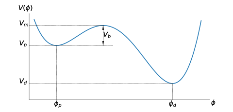
Figure 1: Potential with a true vacuum $V_{d}$ and a false vacuum $V_{p}$.

Consider a scalar field $\phi$ with a double well potential of the form illustrated in Fig. 1. Initially $\phi$ is in the parent vacuum, $\phi_{p}=0$. Suppose that at some time $t_{0}$ the field $\phi$ developed a velocity fluctuation with a spherically symmetric Gaussian profile,

$${\dot{\phi}}(t_{0},r)={\dot{\phi}}_{0}e^{-\frac{r^{2}}{2l^{2}}},$$ (4)

with $\phi(t_{0},r)=\phi_{p}$. In order for the field to fly over the barrier, we need ${\dot{\phi}}^{2}\gtrsim 2V_{b}$, where $V_{b}=V_{m}-V_{p}$ is the height of the barrier, $V_{m}$ is the potential at the top of the barrier and $V_{p}$ is the potential in the parent vacuum. In order for this condition to be satisfied for $r\lesssim l$, we need ${\dot{\phi}}_{0}^{2}\gtrsim 2eV_{b}$.

For $\phi$ near $\phi_{p}$ the potential has the form $V(\phi)\approx m^{2}\phi^{2}/2$, where $m^{2}=V^{\prime\prime}(\phi_{p})$ is the mass parameter of the field in the parent vacuum. For a generic potential we expect $V_{b}\sim m^{2}\Delta\phi^{2}$, where $\Delta\phi$ is the width of the barrier. The bubble wall thickness $\delta$ is determined by the balance between the gradient and potential energies; it can be estimated by minimizing $[(\Delta\phi/\delta)^{2}+V_{b}]\delta$. This gives $\delta\sim\Delta\phi/\sqrt{V_{b}}\sim 1/m$. The wall tension is then $\sigma\sim V_{b}\delta\sim V_{b}/m$.

The force of tension acting per unit area of the bubble wall is $\sigma/R$, and the force due to the difference of vacuum energy densities is $V_{p}-V_{d}\equiv\epsilon$, where $R$ is the bubble radius and $V_{p}$ and $V_{d}$ are the energy densities of the parent and daughter vacua, respectively. For a bubble to expand, its radius should exceed $2\sigma/\epsilon\equiv R_{0}$. A thin-wall bubble with $R_{0}\gg\delta$ corresponds to $V_{b}\gg\epsilon$. The opposite limit, where $V_{b}\ll\epsilon$ and $R_{0}\ll\delta$ will be referred to as a thick-wall bubble.

For a free scalar field the fluctuations are Gaussian and the probability of a velocity fluctuation of magnitude ${\dot{\phi}}_{0}$ on scale $l$ is Huang and Ford (2019)

$$P\sim\exp\left(-\frac{{\dot{\phi}}_{0}^{2}}{2\langle{\dot{\phi}}_{l}^{2}\rangle}\right),$$ (5)

where ${\dot{\phi}}_{l}$ is the field velocity operator smoothed with a Gaussian window of radius $l$ and the angular brackets indicate a vacuum expectation value. Note that this is true due to the fact that the smoothing process preserves the Gaussian nature of the smeared fluctuations. This expectation value is calculated in Appendix A, with the result

$$\langle{\dot{\phi}}_{l}^{2}\rangle\approx\frac{1}{8\pi^{2}l^{4}}$$ (6)

for $ml\ll 1$, and

$$\langle{\dot{\phi}}^{2}_{l}\rangle\approx\frac{m}{16\pi^{3/2}l^{3}}$$ (7)

for $ml\gg 1$. In our case $\phi$ can be accurately approximated as a free field only for $\phi\ll\Delta\phi$, but we shall assume that the above estimates are also correct by order of magnitude for $\phi\sim\Delta\phi$.

In the thin-wall case, the minimal length scale of a fluctuation that can result in an expanding bubble is $l\sim\sigma/\epsilon$. Then $ml\sim V_{b}/\epsilon\gg 1$ and we obtain the following estimate for the transition rate:

$$\kappa\sim\exp\left(-16e\pi^{3/2}\frac{V_{b}l^{3}}{m}\right).$$ (8)

Using $V_{b}/m\sim\sigma$ and $l\sim\sigma/\epsilon$, this can be rewritten as

$$\kappa\sim\exp\left(-16e\pi^{3/2}\frac{\sigma^{4}}{\epsilon^{3}}\right).$$ (9)

In the following subsection we will show a numerical example in this thin-wall limit, where this flyover transition will happen if we take $l\sim 4\sigma/\epsilon$. Apart from the numerical coefficient in the exponent, this agrees with Coleman’s result

$$\kappa_{\rm Coleman}\sim\exp\left(-\frac{27\pi^{2}}{2}\frac{\sigma^{4}}{\epsilon^{3}}\right).$$ (10)

In the thick-wall case, the potential in the vicinity of the barrier can be approximated as

$$V(\phi)\approx\frac{1}{2}m^{2}\phi^{2}-\gamma\phi^{3}$$ (11)

and the tunneling action is Sarid (1998); Dine and Paban (2015)

$$S\approx 24\frac{m^{2}}{\gamma^{2}}.$$ (12)

The height of the barrier in this case is $V_{b}=m^{6}/54\gamma^{2}$ and the minimal fluctuation size is $l\sim\delta\sim 1/m$. More accurately, numerical simulations described in the following subsection indicate that $l\sim 3/m$. Substituting this in the exponent of Eq. (8) gives

$$\ln\kappa\sim 10^{2}\frac{m^{2}}{\gamma^{2}}.$$ (13)

This has the same dependence on the parameters as in (12), but the numerical coefficient is several times larger.

The difference in the numerical coefficient is not surprising if we note that (i) we estimated the length scale $l$ only by order of magnitude and that (ii) we used a free field estimate for the rms velocity fluctuation. Furthermore, we assumed a specific form of the initial fluctuation (with velocity fluctuating and the field value remaining fixed), which is not necessarily the optimal fluctuation resulting in a bubble.

In the above analysis we assumed that the fluctuation keeps its coherence during the transition and obeys the classical field equation. The fluctuation is localized in a region of size $\sim l$ and is composed of the field modes of wavelength $\sim l$ and momentum $k\sim 1/l$. These modes will disperse on a time scale $\tau\sim l/v\sim ml^{2}$, where $v\sim k/m$ is the characteristic velocity. For the fluctuation to remain coherent it is necessary that $\tau\gtrsim\Delta t$, where $\Delta t\sim\Delta\phi/{\dot{\phi}}\sim 1/m$ is the flyover time. This requires that $ml\gtrsim 1$, which is satisfied with a great margin for a thin-wall bubble and is marginally satisfied for a thick-wall bubble. The fluctuation could also disintegrate due to the fact that its constituent modes would oscillate out of phase. But the oscillation frequency is $\sim m$ and once again the dispersion time is $\tau\sim 1/m$.

We note also that bubble nucleation in flat spacetime should conserve energy. On the other hand, the velocity fluctuation (4) has a positive energy ${\cal E}=(2\pi)^{3/2}{\dot{\phi}}_{0}^{2}l^{3}$. This energy should be compensated by a negative energy fluctuation of the vacuum. The mechanism of this energy compensation and its effect on bubble formation require further analysis.

A similar approach can be applied to bubble nucleation at a finite temperature $T$. It is shown in the Appendix that the rms field velocity fluctuation in this case can be represented as a sum of vacuum and thermal contributions,

$$\langle{\dot{\phi}}_{l}^{2}\rangle=\langle{\dot{\phi}}_{l}^{2}\rangle_{v}+\langle{\dot{\phi}}_{l}^{2}\rangle_{T},$$ (14)

where the vacuum contribution is the same as that at $T=0$. At $T\ll m$ the thermal contribution is exponentially suppressed and the nucleation rate is nearly the same as in vacuum. On the other hand, at $T\gg m,1/l$ thermal fluctuations dominate and we find

$$\langle{\dot{\phi}}_{l}^{2}\rangle_{T}\approx\frac{T}{8\pi^{3/2}l^{3}}.$$ (15)

The nucleation rate is then

$$\kappa\sim\exp\left(-8e\pi^{3/2}\frac{V_{b}l^{3}}{T}\right).$$ (16)

Note that ${\cal E}\sim V_{b}l^{3}$ is the energy needed to create a bubble of size $l$ at the top of the barrier, so the right-hand side of (16) can be interpreted as the Boltzmann suppression factor. Once again, the exponent in (16) is parametrically the same as given by the instanton method Linde (1983).

We note finally that the exponents in our estimates of flyover decay rates are consistently greater than those in the tunneling rates calculated by the instanton method, suggesting that flyover is a subdominant decay channel. This conclusion, however, should be taken with caution, since the numerical coefficients in the flyover exponents are not expected to be accurate, for the reasons given above.

II.2 Numerical simulations

In this section, we will numerically investigate the possibility of obtaining an expanding region of true vacuum by the ”flyover” process we discussed earlier. In order to do this we will consider a scalar field with a potential of the form

$$V(\phi)=\frac{1}{2}m^{2}\phi^{2}-\gamma\phi^{3}+\lambda\phi^{4},$$ (17)

where we will vary the parameters in such a way that we will always enforce the presence of two non-degenerate vacua separated by a potential barrier. We will not be concerned with the value of the cosmological constant in each vacuum since in this case we will consider this process in flat space.

As we mentioned earlier we will consider the situation where the initial fluctuation is of the form

$${\dot{\phi}}(t_{0},r)={\dot{\phi}}_{0}e^{-\frac{r^{2}}{2l^{2}}},$$ (18)

where $l$ describes the typical scale of the initial fluctuation and ${\dot{\phi}}_{0}$ denotes the maximum fluctuation amplitude of this initial state. Assuming spherical symmetry we can evolve this initial state by solving the equation

$$\ddot{\phi}-\phi^{\prime\prime}-\frac{2}{r}~{}\phi^{\prime}+\frac{\partial V(\phi)}{\partial\phi}=0~{}.$$ (19)

where we impose the boundary condition at the center of the fluctuation to be such that

$$\phi^{\prime}(r=0)=0$$ (20)

and we take the outer boundary of the simulation box to be fixed at the false vacuum value of the field.

Following Ref. Sarid (1998) we can always rescale the field and the coordinates by the following redefinitions, $\tilde{\phi}=(2\gamma/m^{2})\phi$, $\tilde{x}^{\mu}=(m/\sqrt{2})x^{\mu}$ to obtain a potential that depends only on the dimensionless quantity, $\iota=1-2\lambda m^{2}/\gamma^{2}$, namely,

$$\tilde{V}(\tilde{\phi})=\tilde{\phi}^{2}-\tilde{\phi}^{3}+\frac{1}{4}(1-\iota)\tilde{\phi}^{4},$$ (21)

where $\tilde{V}=(8\gamma^{2}/m^{6})V$. In the following we will investigate two scenarios with different values of $\iota$.

II.2.1 Thin-wall case

Taking the limit of $\iota\rightarrow 0$ the two minima of the potential become degenerate. This corresponds to the thin-wall limit of the usual instanton calculation. The top of the potential is in this case $\tilde{V}_{b}\approx 1/4$, the potential difference in dimensionless units is given by $\tilde{\epsilon}\approx 4\iota$ and the interpolating wall has a tension $\tilde{\sigma}\approx 2\sqrt{2}/3$.

As we described in the previous section, we are interested in studying a fluctuation with a central amplitude given $\dot{\tilde{\phi_{0}}}\approx\left(2e\tilde{V}_{b}\right)^{1/2}\approx\sqrt{e/2}$ and whose scale is of the order of $\tilde{l}\approx C\tilde{\sigma}/\tilde{\epsilon}\approx C\sqrt{2}/(6\iota)$, where $C$ is a numerical coefficient of the order one that we will find from our simulations.

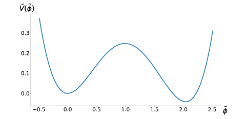
Figure 2: Plot of the potential in Eq. (21) with $\iota=0.01$.

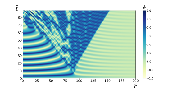
Figure 3: Evolution of the scalar field under the potential with $\iota=0.01$ ($\tilde{\phi}_{d}\approx 2$). The initial fluctuation size is $\tilde{l}=4\tilde{\sigma}/\tilde{\epsilon}\approx 90$. A shell is formed at $\tilde{r}\approx 90$, with the outer boundary propagating outwards and the inner inwards. Both boundaries propagate at a speed close to that of light.

We show in Fig. 3 an example of the evolution of this kind of initial configuration with $\iota=0.01$ (the potential is shown in Fig. 2) and $\tilde{l}=4\tilde{\sigma}/\tilde{\epsilon}$. We can see in the figure that the central region of the fluctuation quickly evolves over the barrier. However, this region is too small to create an expanding bubble. This leads to an oscillating pattern between the false and the true vacuum near the center of the fluctuation.

Further away from the center, the true vacuum is reached later on in the simulation when the interior has already bounced back to the false vacuum. We found that, when the initial size of the fluctuation is large enough, a shell of radius $\sim\tilde{l}$ will form that interpolates between oscillating interior and the parent vacuum outside. The subsequent evolution of this shell is such that its inner boundary propagates inwards and the outer boundary outwards. Both boundaries propagate at a speed close to that of light. For $\iota=0.01$ the smallest $\tilde{l}$ that is able to produce such a shell was found to be $\tilde{l}\approx 4\tilde{\sigma}/\tilde{\epsilon}$.

The field in the expanding shell oscillates around the true vacuum, while in the central region inside of the inner boundary of the shell, it oscillates between the true and the false vacuum.

II.2.2 Thick-wall case

We now study the other end of the spectrum of the possible values of the parameters where the instanton calculation would lead to the formation of a thick bubble. In our parametrization this is achieved by taking the limit of $\iota\rightarrow 1$.

Taking the form of the potential with $\iota=0.96$ (see Fig. 4) we have found that with $\dot{\tilde{\phi_{0}}}=\sqrt{2e\tilde{V}_{b}}$, the smallest fluctuation size that is able to produce a bubble is $\tilde{l}\approx 2.2$. This gives $ml\approx 3$, which leads to our estimate in Eq. (13).

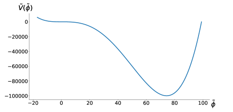
Figure 4: Potential with $\iota=0.96$.

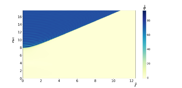
Figure 5: Evolution of the scalar field under the potential with $\iota=0.96$ ($\tilde{\phi}_{d}\approx 74$). The initial fluctuation size is $\tilde{l}=2.2$.

We see in Fig. 5 how, in this case, the initial fluctuation brings a large enough region of space over the barrier, so the resulting bubble of true vacuum is able to expand similarly to what happens in the usual instanton decay.

Since the time it takes for the field at the center to reach the true vacuum is of the order $\Delta\phi/\dot{\phi}_{0}\sim 1/m$ which in this case is $\sim l$, almost the whole fluctuation region gets to the true vacuum simultaneously. As we can see from Fig. 5, the shell structure in the thin-wall case completely disappears, and the field inside the bubble oscillates around the true vacuum.

As a final remark, let us note that rescaling things back we can get a family of solutions with the same kind of behavior as the one given in any of the scenarios presented here but written in terms of the original physical parameters, $m,\gamma$ and $\lambda$.

III Inflating universe

We now turn to flyover transitions in an inflating universe. The potential we consider still has the form shown in Fig. (1). We further assume the height of the barrier to be small compared to the vacuum energy in the parent vacuum, $V_{b}\ll V_{p}$. This ensures that the gravitational back-reaction of the velocity fluctuation is insignificant. Also, in the absence of fine-tuning we expect the mass of the field in the parent vacuum to satisfy $m\gg H_{p}$. Both parent and daughter vacua are de Sitter, so transitions can occur both upwards and downwards.

III.1 Downward transitions

We first consider downward transitions in the case of a small bubble, when the bubble size is small compared to the parent horizon $H_{p}^{-1}$. For a thick-wall bubble this follows from the condition $m\gg H_{p}$, while for a thin-wall bubble this requires $l_{0}\ll H_{p}^{-1}$, where $l_{0}\sim\sigma/\epsilon$ is the flat space bubble size. The minimal velocity necessary to take the field over the barrier is ${\dot{\phi}}_{0}^{2}\sim 2CV_{b}$, where the factor $C>1$ accounts for the Hubble friction. The flyover time is $\Delta t\sim\Delta\phi/{\dot{\phi}}_{0}\sim 1/m\ll 1/H_{p}$. Since it is small compared to the Hubble time, we expect Hubble friction to be insignificant and $C\sim 1$. The rms velocity fluctuation $\langle{\dot{\phi}}^{2}_{l}\rangle$ in dS space is estimated in Appendix A. Somewhat surprisingly, it is given by the same limiting expressions (6), (7) as in flat space, independent of the expansion rate $H_{p}$. Also, for a small bubble, the minimal length scale of the fluctuation needs to be the same as in flat space, that is, $l\sim l_{0}$ and $l\sim 1/m$ for thin-wall and thick-wall bubbles, respectively. The bottom line is that our estimates for the rate of downward transitions are still given by Eqs. (8) and (13), the same as in flat space.

Let us now consider a downward transition with a large bubble, whose size is not small compared to the horizon. This has to be a thin-wall bubble, since the wall thickness is $\delta\sim 1/m\ll H_{p}^{-1}$. Hence we must have $\epsilon\ll V_{b}\ll V_{p}$, so the energy densities of the parent and daughter vacua should be very close to one another: $V_{p}\approx V_{d}$. The minimal size of an inflating bubble in this case is $l\sim H_{p}^{-1}$. Substituting this in Eq. (8) we find

$$\kappa\sim\exp\left(-16e\pi^{3/2}\frac{V_{b}}{mH_{p}^{3}}\right)\sim\exp\left(-16e\pi^{3/2}\sigma H_{p}^{-3}\right).$$ (22)

This can be compared with the instanton calculation of the nucleation rate of domain walls in dS space Basu et al. (1991)

$$\kappa_{\rm wall}\sim\exp\left(-2\pi^{2}\sigma H_{p}^{-3}\right).$$ (23)

(Our process is similar to domain wall nucleation, since $V_{p}\approx V_{d}$.). Once again the two expressions agree, up to a numerical factor in the exponent.

III.2 Upward transitions

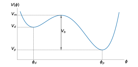
Figure 6: Potential with a true vacuum $V_{p}$ and a false vacuum $V_{d}$.

For an upward transition (Fig. 6), we have $\epsilon\lesssim V_{b}\ll V_{p}$; hence we should have $V_{p}\approx V_{d}$ and $H_{p}\approx H_{d}$. With either relation between $l_{0}$ and $H_{p}^{-1}$, the bubble will inflate only if its size is greater than the horizon, $l\gtrsim H_{p}^{-1}$. The transition rate is then given by Eq. (22). This has some interesting implications.

The upward and downward transition rates can generally be expressed as $\kappa_{\uparrow}\sim e^{-B_{\uparrow}}$ and $\kappa_{\downarrow}\sim e^{-B_{\downarrow}}$, with $B_{\uparrow}\sim\sigma H_{p}^{-3}$ and $B_{\downarrow}\sim\sigma l^{3}$, where $l={\rm min}\{l_{0},H_{p}^{-1}\}$. The ratio of these rates is

$$\frac{\kappa_{\uparrow}}{\kappa_{\downarrow}}=e^{-\Delta B},$$ (24)

where

$$\Delta B=B_{\uparrow}-B_{\downarrow}\lesssim\sigma H_{p}^{-3}.$$ (25)

According to the instanton calculation, this ratio must satisfy the detailed balance condition (3), which requires that $\Delta B=\Delta S$, where

$$\Delta S=S_{p}-S_{d}\sim\frac{\epsilon}{H_{p}^{4}}$$ (26)

is the difference of the de Sitter entropies of the two vacua. Now, from Eqs. (25) and (26) we can write

$$\Delta B\lesssim\frac{l_{0}}{H_{p}^{-1}}\Delta S.$$ (27)

This can be consistent with detailed balance if $l_{0}\gtrsim H_{p}^{-1}$. However, for $l_{0}\ll H_{p}^{-1}$ we have $\Delta B\ll\Delta S$ and the detailed balance is strongly violated. In this case the upward flyover transition rate is much greater than predicted by the instanton formalism.

To be more specific, consider a model where

$$V_{p}-V_{d}\sim V_{b}\ll V_{p}\ll{V_{b}}^{1/2}.$$ (28)

Let us also assume that the barrier is characterized by a single mass scale $m$. Then the flat-space version of this model describes a thick-wall bubble of initial size $l_{0}\sim m^{-1}\sim V_{b}^{-1/4}$, and the last inequality in (28) ensures that $l_{0}\ll H_{p}^{-1}$, where $H_{p}\sim V_{b}^{1/2}$. This implies that the bubble size and the transition amplitude for downward transitions are unaffected by gravity; in particular the bubble size $l$ is close to the flat space value $l_{0}$. The condition of small gravitational back-reaction is also satisfied, and thus we have a well controlled model where detailed balance is strongly violated.

As we already indicated, our analysis cannot be directly extended to large upward jumps with $V_{d}\gg V_{p}$. In this case an inflating bubble can be formed by a fluctuation of size $l\sim H_{d}^{-1}$, which can be much smaller than the parent horizon $H_{p}^{-1}$. This bubble will inflate at a rate much higher than that of the parent vacuum, which is possible geometrically only if the daughter bubble is connected to the parent vacuum by a wormhole. The situation here is similar to baby universe formation from false vacuum bubbles produced during inflation, as discussed in Refs. Garriga et al. (2016); Deng and Vilenkin (2017). It is also similar to the formation of an inflating baby universe in a laboratory, as discussed by Farhi, Guth and Guven Farhi et al. (1990) (See also Garriga and Megevand (2004); Aguirre and Johnson (2006)). The wormhole must close off in about a light crossing time, resulting in an inflating daughter region contained in a baby universe inside a black hole. The mass of the black hole can be estimated as

$$M\sim V_{d}H_{d}^{-3}\sim H_{d}^{-1}.$$ (29)

This scenario is confirmed by a numerical simulation described in the next subsection.

We cannot reliably estimate the rate of large upward transitions, since such transitions would induce a large gravitational back-reaction. As a plausible guess, one can expect that it is comparable to the nucleation rate of black holes of mass (29) in the parent dS space:

$$\kappa\sim\exp\left(-\frac{M}{T}\right)\sim\exp\left(-\frac{C}{H_{d}H_{p}}\right).$$ (30)

Here $T=H_{p}/2\pi$ is the Gibbons-Hawking temperature of the parent vacuum and $C$ is a numerical coefficient ${\cal O}(1)$. Once again, this rate is much higher than the estimate based on the Lee-Weinberg instanton,

$$\kappa_{LW}\sim\exp\left(-\frac{\pi}{H_{p}^{2}}\right).$$ (31)

III.3 Numerical simulations of upward transitions

We will now present some numerical results of the upward transitions discussed in the last subsection, where the background is inflating and gravity can no longer be neglected. We solve the scalar field equation together with Einstein’s equations for the spherically symmetric initial fluctuation of the form given by Eq. (4).

The metric we consider is

$$ds^{2}=-dt^{2}+B^{2}dr^{2}+R^{2}d\Omega^{2},$$ (32)

where $d\Omega^{2}$ is the metric on a unit sphere and $B$ and $R$ (which is called the area radius) are functions of the coordinates $t$ and $r$. We give in Appendix B a detailed account of the numerical implementation of this system of equations as well as the method we use to impose the initial conditions.

Specifically, we will use several examples to illustrate the flyover upward transitions in two cases: (i) $V_{d}\sim V_{p}\gg V_{b}$, where the background can be regarded as fixed dS; and (ii) $V_{d}\sim V_{b}\gg V_{p}$, where strong gravitational back-reaction is expected.

III.3.1 $V_{d}\sim V_{p}\gg V_{b}$

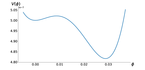
Figure 7: Potential with $V_{d}\sim V_{p}\gg V_{b}$

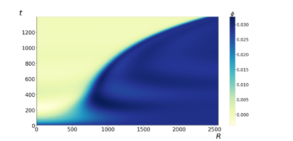
Figure 8: Evolution of the scalar field under the potential Fig. 7, with $l=H_{d}^{-1}\approx 490$ and $\dot{\phi}_{0}=-1.8\sqrt{2V_{b}}$. The horizontal axis is the area radius $R$ and the vertical axis is time $t$. We can clearly see the formation and growth of a false vacuum bubble.

As before, we consider a scalar field with a potential in the form of Eq. (17),

$$V(\phi)=10^{-8}[(100\phi)^{2}-(100\phi)^{3}+0.2(100\phi)^{4}]+5\times 10^{-7},$$ (33)

where the parameters have been chosen such that we fullfill the requirements given above together with the condition $m\gg H_{p}$ while still being in a sub-Planckian regime. In particular we get $m^{-1}\approx 46$, $l_{0}\approx 225$, $H_{p}^{-1}\approx 500$ and $H_{d}^{-1}\approx 490$. We show the form of this potential in Fig. 7 where we can see that the energy difference between the two vacua is small compared to their absolute values.

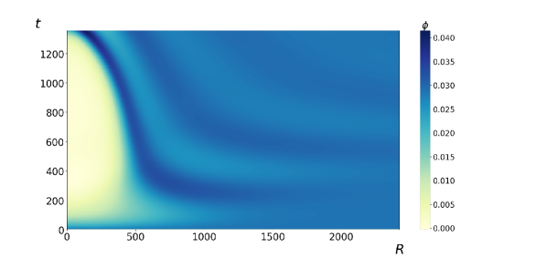
Figure 9: Evolution of the scalar field under the potential Fig. 7, with $l=H_{d}^{-1}\approx 490$ and $\dot{\phi}_{0}=-1.6\sqrt{2V_{b}}$. The horizontal axis is the area radius $R$ and the vertical axis is time $t$. A false vacuum bubble forms and then collapses.

We show in Fig. 8 an example of the field evolution obtained using the equations in the Appendix. The field is initially in the true vacuum everywhere, $\phi(t_{0},r)\approx 0.029$, but the velocity field has a spherically symmetric fluctuation with $l=H_{d}^{-1}$ and $\dot{\phi}_{0}=-1.8\sqrt{2V_{b}}$. It can be seen that, as the field at the center of the fluctuation flies over the barrier and reaches the false vacuum valley, a bubble is formed and starts to grow exponentially. This confirms our theoretical expectations from the previous section.

If the magnitude (or the size) of the field velocity fluctuation is not large enough, even if the field near the center flies over the barrier and form a bubble, the bubble would eventually shrink and disappear. Fig. 9 shows such a case with $l=H_{d}^{-1}$ and $\dot{\phi}_{0}=-1.6\sqrt{2V_{b}}$. The initial fluctuation has the same size as the one that gives Fig. 8, but a smaller magnitude. This case is nearly critical. As we can see from Fig. 9, the bubble reaches a size close to the daughter horizon $H_{d}^{-1}\approx 490$, which means gravity almost defeats pressure and creates an inflating region. But the bubble ends up collapsing.

III.3.2 $V_{d}\sim V_{b}\gg V_{p}$

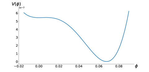
Figure 10: Potential with $V_{d}\sim V_{b}\gg V_{p}$

As discussed in the previous subsection, it would be interesting to numerically investigate the case where the expansion rate of the daughter vacuum is much larger than that in the parent vacuum. The potential we consider for this case is given by,

$$V(\phi)=10^{-8}[(100\phi)^{2}-(100\phi)^{3}+0.1(100\phi)^{4}]+5.44\times 10^{-7},$$ (34)

which is shown in Fig. 10. In this potential $m^{-1}\approx 25$, $H_{p}^{-1}\approx 3.7\times 10^{4}$ and $H_{d}^{-1}\approx 470$. As before, the field is initially in the true vacuum, $\phi(t_{0},r)\approx 0.068$ and the fluctuation parameters are $l=2.7H_{d}^{-1}\ll H_{p}^{-1}$ and $\dot{\phi}_{0}=-1.3\sqrt{2V_{b}}$.

We show in Fig. 11 the field evolution in this case where the fluctuation is strong enough to bring the field over the barrier and create a bubble of the false vacuum. We note that the size of this bubble is of the order of $H_{d}^{-1}$ and much smaller than $H_{p}^{-1}$ and once formed it does not collapse. This example shows that upward transitions of this type indeed seem to happen in a curved spacetime.

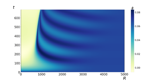
Figure 11: Evolution of the scalar field under the potential Fig. 10, with $l=2.7H_{d}^{-1}$ and $\dot{\phi}_{0}=-1.3\sqrt{2V_{b}}$. The horizontal axis is the area radius $R$ and the vertical axis is time $t$. A false vacuum bubble forms and expands.

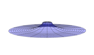
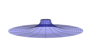
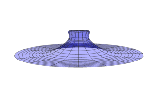
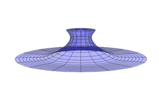
Figure 12: Embedding diagrams at different moments showing how the wormhole develops. The flat-looking region at the top and the bottom area represent the daughter and parent regions respectively. The ring that encircles the cap is the bubble wall. The arc length from the cap center along longitude is the proper radius $d(r)\equiv\int_{0}^{r}B(\tilde{r})d\tilde{r}$, while the radius of a latitude circle is the area radius $R$.

The exponentially growing stage is not shown in Fig. 11 due to the formation of a wormhole geometry. Since the expansion rate of the false vacuum is much larger than that in the background, the bubble inflates into a baby universe, which is connected to the parent universe by a wormhole. After the wormhole is formed, the area radius $R$ is no longer a monotonic function of the coordinate $r$ (hence it can no longer serve as the horizontal axis in Fig. 11) but has a local minimum, which is the wormhole throat. This throat would eventually close off and the wormhole would turn into a Schwarzschild-de Sitter black hole for an observer in the parent universe. In the above example, our simulation shows that the resulting black hole has mass $M\approx 750$. This is consistent with the estimate (29). In Fig. 12 we show the wormhole formation by its embedding diagrams at four different moments.

IV Conclusions

We used analytic and numerical methods to investigate flyover vacuum transitions in flat and dS space. Our numerical simulations indicate that the dynamics of bubble nucleation and early evolution in these transitions can be rather different from the standard picture. The difference is most pronounced for thin-wall bubbles, where the transition region undergoes a number of oscillations between true and false vacuum, until a true vacuum shell is formed which expands both inwards and outwards. This suggests that flyover transitions provide another channel of vacuum decay, different from quantum tunneling. Our analytic estimates of flyover decay rates in flat space and of downward decays in dS space have the same parametric dependence as given by the instanton method for tunneling transitions, with a numerical coefficient in the exponent different by a factor ${\cal O}(1-10)$. The estimates suggest that the flyover rate is smaller than the tunneling rate, although their accuracy is not sufficient to establish this with certainty. If the flyover decays are indeed subdominant, the standard results for the vacuum decay rate would still apply.

On the other hand, for upward transitions in dS space the flyover decay rate is parametrically different from tunneling and can be higher by many orders of magnitude. This is an interesting result, which implies in particular that the detailed balance condition (3) is violated. If correct, this violation would be a significant deviation from the conventional picture of quantum dS space as a thermal state Dyson et al. (2002).

Another important difference from the standard picture is that unlike Coleman’s or the CdL bubbles, flyover vacuum transitions are not symmetric with respect to Lorentz or de Sitter boosts. There is a preferred frame where the fluctuation is spherically symmetric, which can be regarded as the rest frame of bubble nucleation. This is not necessarily a problem, since a metastable vacuum always has a preferred frame, which is set by the way the vacuum was created and which manifests itself for example by the ”persistence of memory” effect Garriga et al. (2007).

In most of our analysis we assumed that the tunneling barrier height is small compared to the parent vacuum energy density, $V_{b}\ll V_{p}$, to ensure that gravitational back-reaction of the initial fluctuation is small. We also considered upward dS transitions where the daughter vacuum has a much higher energy density than the parent vacuum, $V_{d}\gg V_{p}$. Then we must also have $V_{b}\gg V_{p}$ and the transition rate cannot be reliably estimated. We expect, however, the rate to be nonzero and we performed numerical simulations of flyover transitions in this case. We find that after the transition the rapidly inflating daughter region is connected to the parent vacuum by a wormhole. The wormhole closes off in about a light crossing time, resulting in an inflating daughter bubble contained in a baby universe inside of a black hole.

In this paper we focused on flyover transitions for which an alternative CdL tunneling transition is also possible. We note however that there are generic situations where CdL instantons do not exist. For example, tunneling between two dS vacua may not be possible if there is an Anti de Sitter (AdS) or Minkowski vacuum between them. This could actually be the case for most dS vacuum pairs in the Landscape Blanco-Pillado et al. (2019). In such cases a flyover transition may be the only available vacuum decay channel. These types of transitions could also be relevant in the calculation of the spectrum of primordial black holes produced during inflation in scenarios previously discussed in Refs. Garriga et al. (2016); Deng and Vilenkin (2017).

We finally emphasize that our approach to estimating the transition rates is heuristic in nature. We used quantum field theory to estimate the probability of the initial fluctuation and then evolved the fluctuation using the classical field equations. Justification of this method from first principles and determining the limits of its applicability remain problems for future research. Some steps in this direction, using the Wigner distribution functions, were taken in Ref. Braden et al. (2018); Hertzberg and Yamada (2019).

V Acknowledgements

We are grateful to Adam Brown, Larry Ford, Haiyun Huang, Matthew Johnson, Matthew Kleban and Ken Olum for very useful discussions. J. J. B.-P. is supported in part by the Spanish Ministry MINECO grant (FPA2015-64041-C2-1P), the MCIU/AEI/FEDER grant (PGC2018-094626-B-C21), the Basque Government grant (IT-979-16) and the Basque Foundation for Science (IKERBASQUE). H. D. and A. V. are supported by the National Science Foundation under grant PHY-1820872.

Appendix A

Here we find the rms magnitude of field velocity fluctuations in Minkowski and de Sitter space.

A.1 Minkowski space

A free scalar field of mass $m$ in Minkowski space is represented by a field operator

$${\hat{\phi}}({\bf x},t)=(2\pi)^{-3/2}\int d^{3}k\left[{\hat{a}}_{\bf k}\psi_{k}(t)e^{i{\bf kx}}+{\hat{a}}^{\dagger}_{\bf k}\psi^{*}_{k}(t)e^{-i{\bf kx}}\right],$$ (35)

where the annihilation and creation operators ${\hat{a}},{\hat{a}}^{\dagger}$ satisfy the standard commutation relations, $\psi_{k}(t)=(2E_{k})^{-1/2}e^{-iE_{k}t}$, $E_{k}=\sqrt{k^{2}+m^{2}}$ and $k=|{\bf k}|$. We define a velocity operator smeared over distance scale $l$:

$${\dot{\hat{\phi}}}_{l}({\bf x},t)=(2\pi d^{2})^{-3/2}\int d^{3}x^{\prime}{\dot{\hat{\phi}}}({\bf x},t)\exp\left(-\frac{|{\bf x}-{\bf x}^{\prime}|^{2}}{2l^{2}}\right).$$ (36)

We are interested in the quantity

$$\langle{\dot{\phi}}_{l}^{2}\rangle\equiv\langle 0|{\dot{\hat{\phi}}}_{l}^{2}({\bf x},t)|0\rangle=\frac{1}{4\pi^{2}}\int_{0}^{\infty}e^{-k^{2}l^{2}}E_{k}k^{2}dk=\frac{(ml)^{2}e^{(ml)^{2}}}{16\pi^{2}l^{4}}K_{1}(ml/2)$$ (37)

where we have introduced $K_{1}(x)$ which denotes a modified Bessel function. For $ml\gg 1$ we can approximate $E_{k}\approx m$; this gives in this limit,

$$\langle{\dot{\phi}}_{l}^{2}\rangle\approx\frac{m}{16\pi^{3/2}l^{3}}.$$ (38)

In the opposite limit, $ml\ll 1$, $E_{k}\approx k$ and we have

$$\langle{\dot{\phi}}_{l}^{2}\rangle\approx\frac{1}{8\pi^{2}l^{4}}.$$ (39)

A.2 Finite temperature

In a thermal state at temerature $T$ we have $\langle a^{\dagger}a\rangle=n_{k}$ and Eq. (37) is replaced by

$$\langle{\dot{\phi}}_{l}^{2}\rangle=\frac{1}{4\pi^{2}}\int_{0}^{\infty}e^{-k^{2}l^{2}}(1+2n_{k})E_{k}k^{2}dk=\langle{\dot{\phi}}_{l}^{2}\rangle_{v}+\langle{\dot{\phi}}_{l}^{2}\rangle_{T}.$$ (40)

Here, angular brackets indicate averaging with a thermal density matrix, $n_{k}=\left(e^{E_{k}/T}-1\right)^{-1}$ is the Bose distribution function, and the two terms on the right-hand side represent vacuum and thermal contributions. The vacuum contribution is the same as at $T=0$ and the thermal contribution is

$$\langle{\dot{\phi}}_{l}^{2}\rangle_{T}=\frac{1}{2\pi^{2}}\int_{0}^{\infty}e^{-k^{2}l^{2}}\frac{E_{k}k^{2}dk}{e^{E_{k}/T}-1}.$$ (41)

For $T\ll m$ the thermal contribution is exponentially suppressed, $\langle{\dot{\phi}}_{l}^{2}\rangle_{T}\propto e^{-m/T}$. On the other hand, at $T\gg m,1/l$ we have

$$\langle{\dot{\phi}}_{l}^{2}\rangle_{T}\approx\frac{T}{2\pi^{2}}\int_{0}^{\infty}e^{-k^{2}l^{2}}k^{2}dk=\frac{T}{8\pi^{3/2}l^{3}}.$$ (42)

This is much larger than the vacuum contribution (38); hence thermal fluctuations dominate in this regime.

A.3 de Sitter space

We now consider a scalar field in dS space,

$$ds^{2}=a^{2}(\eta)\left(d\eta^{2}-d{\bf x}^{2}\right),$$ (43)

where $a(\eta)=-(H\eta)^{-1}$. The time variable $\eta$ varies in the range $-\infty<\eta<0$ and is related to the proper time $t$ by $dt=-a(\eta)d\eta$. A free scalar field operator in dS space can be represented as

$${\hat{\phi}}(x)=(2\pi)^{-3/2}\int d^{3}k\left[{\hat{a}}_{\bf k}\psi_{k}(\eta)e^{i{\bf kx}}+{\hat{a}}^{\dagger}_{\bf k}\psi^{*}_{k}(\eta)e^{-i{\bf kx}}\right],$$ (44)

Assuming that the field is in a Bunch-Davies vacuum state, the mode functions are given by

$$\psi_{k}(\eta)=\frac{\sqrt{\pi}H}{2}e^{\frac{i\pi\mu}{2}}(-\eta)^{3/2}H_{\mu}^{(1)}(-k\eta),$$ (45)

where $H_{\mu}^{(1)}(x)$ are the Hankel functions and

$$\mu=\sqrt{\frac{9}{4}-\frac{m^{2}}{H^{2}}}.$$ (46)

The smeared velocity operator is given by

$${\dot{\hat{\phi}}}_{l}({\bf x},\eta)=(2\pi d^{2})^{-3/2}\int d^{3}x^{\prime}{\dot{\hat{\phi}}}({\bf x},\eta)\exp\left(-\frac{|{\bf x}-{\bf x}^{\prime}|^{2}}{2H^{2}\eta^{2}l^{2}}\right),$$ (47)

where dots stand for derivatives with respect to the proper time $t$ and $l$ is the physical smearing length. The rms field velocity fluctuation is characterized by the vacuum expectation value

$${\dot{\phi}}^{2}_{l}\equiv\langle 0|{\dot{\hat{\phi}}}_{l}^{2}({\bf x},\eta)|0\rangle=\frac{H^{2}\eta^{2}}{2\pi^{2}}\int_{0}^{\infty}dkk^{2}\left|\frac{d\psi_{k}}{d\eta}\right|^{2}e^{-{H^{2}\eta^{2}k^{2}l^{2}}}.$$ (48)

We are interested in the case when $m\gg H$. Then $\mu\approx im/H\equiv i\nu$. The mode functions in this regime can be found using the integral representation of the Hankel functions,

$$H_{i\nu}^{(1)}(x)=\frac{1}{i\pi}e^{\frac{\pi\nu}{2}}\int_{-\infty}^{\infty}d\xi e^{i(x\cosh\xi-\nu\xi)}.$$ (49)

For $\nu\gg 1$ the integral in (49) can be evaluated using the stationary phase approximation; this gives

$$H_{i\nu}^{(1)}(x)\approx\sqrt{\frac{2}{i\pi}}e^{\frac{\pi\nu}{2}}(x^{2}+\nu^{2})^{-1/4}e^{if(x)},$$ (50)

where

$$f(x)=\sqrt{x^{2}+\nu^{2}}-\nu\ln\frac{x+\sqrt{x^{2}+\nu^{2}}}{\nu}.$$ (51)

The integral over $k$ in Eq. (48) is dominated by the values $k\sim 1/H\eta l$. For $ml\ll 1$ this corresponds to the argument of the Hankel function $k|\eta|\gg\nu$. Then

$$\psi_{k}(\eta)\approx\frac{H|\eta|}{\sqrt{2ik}}e^{-ik\eta}$$ (52)

and

$$\langle{\dot{\phi}}^{2}_{l}\rangle\approx\frac{H^{4}\eta^{4}}{4\pi^{2}}\int_{0}^{\infty}dkk^{3}e^{-{H^{2}\eta^{2}k^{2}l^{2}}}=\frac{1}{8\pi^{2}l^{4}}.$$ (53)

As one might expect, ${\dot{\phi}}^{2}_{l}$ is independent of time $\eta$. In the opposite regime, $ml\gg 1$, we have

$$\psi_{k}(\eta)\approx\frac{H}{\sqrt{2i\nu}}(-\eta)^{3/2}e^{i\nu\left(1+\ln\frac{k|\eta|}{2\nu}\right)}$$ (54)

and

$$\langle{\dot{\phi}}^{2}_{l}\rangle\approx\frac{m}{16\pi^{3/2}l^{3}}.$$ (55)

Somewhat surprisingly, these results are the same as in Minkowski space in both limiting cases.

As an independent check of Eq. (54) we note that it can be rewritten as

$$\psi_{k}(t)\approx\frac{1}{\sqrt{2m}}[a(t)]^{-3/2}e^{-imt+i\alpha_{k}},$$ (56)

where $a(t)=e^{Ht}=(H|\eta)^{-1}$ is the scale factor and $\alpha_{k}$ is a constant phase. This form of the mode functions can also be obtained by solving the field equation

$${\ddot{\psi}}_{k}+3H{\dot{\psi}}_{k}+k^{2}a^{-2}(t)\psi_{k}+m^{2}\psi_{k}=0.$$ (57)

For $ml\gg 1$ the relevant mode functions are the ones with $k/a\ll m$, so the gradient term in (57) can be neglected and the solution is (for $m\gg H$)

$$\psi_{k}(t)\approx A_{k}a^{-3/2}e^{-imt}.$$ (58)

The normalization constant $A_{k}$ can be found from the condition

$$\psi_{k}{\dot{\psi}}^{*}_{k}-\psi^{*}_{k}{\dot{\psi}}_{k}=ia^{-3}.$$ (59)

This gives $|A_{k}|\approx(2m)^{-1/2}$, and thus we recover Eq. (54).

We have also verified numerically that Eqs. (50), (51) give a good fit to Hankel functions of large imaginary order.

Appendix B

In this appendix we outline the setup of our simulations used to illustrate the upward transitions between dS vacua when gravity is taken into account.

Consider a general spherically symmetric metric

$$ds^{2}=-dt^{2}+B^{2}dr^{2}+R^{2}d\Omega^{2},$$ (60)

where $d\Omega^{2}$ is the metric on a unit sphere and $B$ and $R$ are functions of the coordinates $t$ and $r$. For later convenience, we define

$$U=\dot{R},~{}~{}~{}~{}~{}\Gamma=\frac{R^{\prime}}{B},~{}~{}~{}~{}~{}K=\frac{\dot{B}}{B}+\frac{2\dot{R}}{R}.$$ (61)

The Lagrangian density of a scalar field $\phi$ with potential $V(\phi)$ is

$$\mathcal{L}=\frac{1}{2}(\partial\phi)^{2}-V(\phi),$$ (62)

and the corresponding energy-momentum tensor is given by

$$-T^{0}_{\ 0}=\frac{1}{2}\dot{\phi}^{2}+\frac{1}{2}\left(\frac{\phi{\prime}}{B}\right)^{2}+V(\phi),$$ (63)

$$T^{1}_{\ 1}=\frac{1}{2}\dot{\phi}^{2}+\frac{1}{2}\left(\frac{\phi{\prime}}{B}\right)^{2}-V(\phi),$$ (64)

$$T^{2}_{\ 2}=\frac{1}{2}\dot{\phi}^{2}-\frac{1}{2}\left(\frac{\phi{\prime}}{B}\right)^{2}-V(\phi),$$ (65)

$$T^{0}_{\ 1}=\dot{\phi}\phi^{\prime}.$$ (66)

Using Einstein’s equations and the scalar field equation we obtain,

$$\dot{K}=-\left(K-\frac{2U}{R}\right)^{2}-2\left(\frac{U}{R}\right)^{2}-4\pi(T_{\ 1}^{1}+2T_{\ 2}^{2}-T_{\ 0}^{0})$$ (67)

$$\dot{U}=-\frac{1-\Gamma^{2}+U^{2}}{2R}-4\pi RT_{\ 1}^{1}$$ (68)

$$\dot{\Gamma}=-\frac{4\pi RT_{\ 1}^{0}}{B}$$ (69)

$$\dot{B}=B\left(K-\frac{2U}{R}\right)$$ (70)

$$\dot{R}=U$$ (71)

$$\ddot{\phi}=-K\dot{\phi}+\frac{1}{BR^{2}}\left(\frac{R^{2}}{B}\phi^{\prime}\right)^{\prime}-\partial_{\phi}V$$ (72)

which are the evolution equations for the functions $K,\ U,\ \Gamma,\ B,\ R$ and $\phi$.

To evolve this system we need initial and boundary conditions of the equations. The initial profile of the scalar field and that of the field velocity are respectively set to be

$$\phi(r)=\phi_{p},~{}~{}~{}~{}~{}\dot{\phi}(r)=\dot{\phi}_{0}e^{-\frac{r^{2}}{2l^{2}}},$$ (73)

where $\phi_{p}$ is the field value at true (parent) vaccum and $l$ characterizes the width of the velocity fluctuation. The initial energy density is given by $\rho(r)\equiv-T_{\ 0}^{0}=\dot{\phi}^{2}_{0}e^{-\frac{r^{2}}{l^{2}}}/2+V(\phi_{p})$.

As for the metric functions at the initial time, we set $B(r)=1$ and $R(r)=r$. Then by definition we have $\Gamma(r)=1$. The mass enclosed by a certain sphere is characterized by the Misner-Sharp mass, which in our coordinates is

$$M(r)=\frac{R}{2}\left(1-\Gamma^{2}+U^{2}\right).$$ (74)

From $G_{00}\propto T_{00}$, we have $M^{\prime}(r)=4\pi\rho R^{2}R^{\prime}$, which gives

$$M(r)=4\pi\int\rho r^{2}dr.$$ (75)

This can be found by numerical integration. Then by the definition of the Misner-Sharp mass, the initial profile of $U$ is

$$U(r)=\sqrt{\frac{2M}{r}},$$ (76)

where we have used $\Gamma=1$. From $G_{01}\propto T_{01}$, it can be shown that

$$\frac{\dot{B}}{B}=\frac{U^{\prime}}{R^{\prime}}=\frac{2\pi\rho r^{\frac{3}{2}}}{\sqrt{M/2}}-\frac{\sqrt{M/2}}{r^{\frac{3}{2}}}.$$ (77)

Therefore, by definition, the initial profile of $K$ is given by

$$K(r)=\frac{2\pi\rho r^{\frac{3}{2}}}{\sqrt{M/2}}+\frac{3\sqrt{M/2}}{r^{\frac{3}{2}}}.$$ (78)

Following this procedure we can obtain all the initial conditions needed for our system of equations.

The boundary conditions (at $r\to 0$ and $r\to\infty$) are easy to impose, and will not be listed here.

The formation of a black hole can be indicated by the appearance of a black hole apparent horizon, on which we have

$$U+\Gamma=0,~{}~{}~{}~{}~{}U-\Gamma<0$$ (79)

in our coordinates. Then the black hole mass can be read as the Misner-Sharp mass on the horizon, $M=R/2$. More details can be found in Ref. Deng and Vilenkin (2017) and references therein.

References

- Ellis et al. (1990) J. R. Ellis, A. D. Linde, and M. Sher, Phys. Lett. B252, 203 (1990).
- Linde (1992) A. D. Linde, Nucl. Phys. B372, 421 (1992), eprint hep-th/9110037.
- Brown and Dahlen (2011) A. R. Brown and A. Dahlen, Phys. Rev. Lett. 107, 171301 (2011), eprint 1108.0119.
- Braden et al. (2018) J. Braden, M. C. Johnson, H. V. Peiris, A. Pontzen, and S. Weinfurtner (2018), eprint 1806.06069.
- Huang and Ford (2019) H. Huang and L. H. Ford, work in progress (2019), seminar given by H. Huang at Tufts University, April 2018.
- Hertzberg and Yamada (2019) M. P. Hertzberg and M. Yamada (2019), eprint 1904.08565.
- Coleman (1977) S. R. Coleman, Phys. Rev. D15, 2929 (1977), [Erratum: Phys. Rev.D16,1248(1977)].
- Coleman and De Luccia (1980) S. R. Coleman and F. De Luccia, Phys. Rev. D21, 3305 (1980).
- Lee and Weinberg (1987) K.-M. Lee and E. J. Weinberg, Phys. Rev. D36, 1088 (1987).
- Hawking and Moss (1982) S. W. Hawking and I. G. Moss, Phys. Lett. 110B, 35 (1982), [Adv. Ser. Astrophys. Cosmol.3,154(1987)].
- Dyson et al. (2002) L. Dyson, M. Kleban, and L. Susskind, JHEP 10, 011 (2002), eprint hep-th/0208013.
- Sarid (1998) U. Sarid, Phys. Rev. D58, 085017 (1998), eprint hep-ph/9804308.
- Dine and Paban (2015) M. Dine and S. Paban, JHEP 10, 088 (2015), eprint 1506.06428.
- Linde (1983) A. D. Linde, Nucl. Phys. B216, 421 (1983), [Erratum: Nucl. Phys.B223,544(1983)].
- Basu et al. (1991) R. Basu, A. H. Guth, and A. Vilenkin, Phys. Rev. D44, 340 (1991).
- Garriga et al. (2016) J. Garriga, A. Vilenkin, and J. Zhang, JCAP 1602, 064 (2016), eprint 1512.01819.
- Deng and Vilenkin (2017) H. Deng and A. Vilenkin, JCAP 1712, 044 (2017), eprint 1710.02865.
- Farhi et al. (1990) E. Farhi, A. H. Guth, and J. Guven, Nucl. Phys. B339, 417 (1990).
- Garriga and Megevand (2004) J. Garriga and A. Megevand, Int. J. Theor. Phys. 43, 883 (2004), eprint hep-th/0404097.
- Aguirre and Johnson (2006) A. Aguirre and M. C. Johnson, Phys. Rev. D73, 123529 (2006), eprint gr-qc/0512034.
- Garriga et al. (2007) J. Garriga, A. H. Guth, and A. Vilenkin, Phys. Rev. D76, 123512 (2007), eprint hep-th/0612242.
- Blanco-Pillado et al. (2019) J. J. Blanco-Pillado, H. Deng, and A. Vilenkin, work in progress (2019).