Poiseuille flow of nematic liquid crystals via the full Ericksen-Leslie model

Abstract.

In this paper, we study the Cauchy problem of the Poiseuille flow of the full Ericksen-Leslie model for nematic liquid crystals. The model is a coupled system of a parabolic equation for the velocity and a quasilinear wave equation for the director. For a particular choice of several physical parameter values, we construct solutions with smooth initial data and finite energy that produce, in finite time, cusp singularities – blowups of gradients. The formation of cusp singularity is due to local interactions of wave-like characteristics of solutions, which is different from the mechanism of finite time singularity formations for the parabolic Ericksen-Leslie system. The finite time singularity formation for the physical model might raise some concerns for purposes of applications. This is, however, resolved satisfactorily; more precisely, we are able to establish the global existence of weak solutions that are Hölder continuous and have bounded energy. One major contribution of this paper is our identification of the effect of the flux density of the velocity on the director and the reveal of a singularity cancellation – the flux density remains bounded while its two components approach infinity at formations of cusp singularities.

2010 Mathematical Subject Classification: 35M31, 35L52, 35L67, 76D03.

Key Words: Liquid crystal, flux density, global existence, cusp singularity.

1. Introduction

In this paper, we consider singularity formation and global existence of Hölder continuous weak solution for the Cauchy problem

$$\begin{split}u_{t}=&(u_{x}+\theta_{t})_{x},\\ \theta_{tt}+2\theta_{t}=&c(\theta)(c(\theta)\theta_{x})_{x}-u_{x}.\end{split}$$ (1.1)

with initial data

$$u(x,0)=u_{0}(x)\in H^{1}(\mathbb{R}),\quad\theta(x,0)=\theta_{0}(x)\in H^{1}(\mathbb{R}),\quad\theta_{t}(x,0)=\theta_{1}(x)\in L^{2}(\mathbb{R}).$$ (1.2)

In addition, we assume that, for some $\alpha>0$,

$$u^{\prime}_{0}(x)+\theta_{1}(x)\in L^{\infty}\cap C^{\alpha}(\mathbb{R})\;\hbox{ and}\;\lim_{|x|\rightarrow\infty}(\theta_{1},\theta^{\prime}_{0},u^{\prime}_{0})(x)=0.$$ (1.3)

We also assume that the function $c(\cdot)$ is $C^{2}$, and there exist positive constants $C_{L}$, $C_{U}$ and $C_{1}$ such that,

$$0<C_{L}\leq c(\cdot)\leq C_{U}<\infty,\quad|c^{\prime}(\cdot)|\leq C_{1}.$$ (1.4)

System (1.1) is the full Ericksen-Leslie model for Poiseuille flow of nematic liquid crystals with a particular choice of parameters. The general model for Poiseuille flow of nematics and the choice of parameters that leads to system (1.1) will be discussed in Section 2.1.

For system (1.1), we will show by a class of examples that (one-sided) cusp singularity can be formed in finite time and, taking this into consideration, we are still able to establish the global existence of weak solutions with a bounded energy. Although we do not work on the model for Poiseuille flow of nematics with general parameters in this paper, we believe that the similar results hold true in general.

We will next recall the Ericksen-Leslie model followed by a discussion of some relevant results to this work. Experts in this field can skip Section 1.1 and jump to Section 1.2.

1.1. Ericksen-Leslie model for nematic liquid crystals

Liquid crystals are intermediate phases between solid and isotropic fluid. Liquid crystal materials have a degree of crystal structures but also exhibit many hydrodynamic features so they are capable to flow. These multi-facet properties are very important to present applications of display and many yet to come. Nematic liquid crystals are composed of rod-like molecules characterized by average alignment of the long axes of neighboring molecules, which have simplest structures among liquid crystals and have been widely studied analytically and experimentally that lead to fruitful applications ([14, 10, 15, 27]). The modeling and analysis of the nematic liquid crystals have attracted a lot of interests of mathematicians for several decades.

If the orientation order parameters of nematic materials are treated as a unit vector ${{\bf n}}\in\mathbb{S}^{2}$, the director, then the Oseen-Frank energy density determines the macrostructure of the crystal structure ([38, 17])

$$\begin{split}2W({\bf n},\nabla{\bf n})=&K_{1}(\mbox{div\,}{\bf n})^{2}+K_{2}({\bf n}\cdot\mbox{curl\,}{\bf n})^{2}+K_{3}|{\bf n}\times\mbox{curl\,}{\bf n}|^{2}\\ &+(K_{2}+K_{4})[\mbox{tr}(\nabla{\bf n})^{2}-(\mbox{div\,}{\bf n})^{2}]\end{split}$$ (1.5)

where $K_{j}$, $j=1,2,3$, are the positive constants representing splay, twist, and bend effects respectively, with $K_{2}\geq|K_{4}|$, $2K_{1}\geq K_{2}+K_{4}$. (One often takes $K_{2}+K_{4}=0$.) The equilibrium theory of nematics is the variational problem of the total Oseen-Frank energy over the domain $\Omega\subset\mathbb{R}^{3}$ occupied by the material. The theory has been developed successfully and gives a wide range of interesting properties [19, 33, 36].

The hydrodynamic property of nematics is macroscopically characterized by the velocity field ${\bf u}$. Any distortion of the director ${\bf n}$ causes the flow and, likewise, any flow affects the alignment ${\bf n}$. These influences are determined by the the kinematic transport tensor $g$ and the viscous stress tensor $\sigma$ given below. Let

$$D=\frac{1}{2}(\nabla{\bf u}+\nabla^{T}{\bf u}),\quad\omega=\frac{1}{2}(\nabla{\bf u}-\nabla^{T}{\bf u}),\quad N=\dot{\bf n}-\omega{\bf n},$$

represent the rate of strain tensor, skew-symmetric part of the strain rate, and the rigid rotation part of director changing rate by fluid vorticity, respectively. The kinematic transport ${\bf g}$ is given by

$${\bf g}=\gamma_{1}N+\gamma_{2}D{\bf n}$$ (1.6)

which represents the effect of the macroscopic flow field on the microscopic structure. The material coefficients $\gamma_{1}$ and $\gamma_{2}$ reflect the molecular shape and the slippery part between fluid and particles. The first term of ${\bf g}$ represents the rigid rotation of molecules, while the second term stands for the stretching of molecules by the flow. The viscous (Leslie) stress tensor $\sigma$ has the following form

$$\begin{split}\sigma=&\alpha_{1}({\bf n}^{T}D{\bf n}){\bf n}\otimes{\bf n}+\alpha_{2}N\otimes{\bf n}+\alpha_{3}{\bf n}\otimes N\\ &+\alpha_{4}D+\alpha_{5}(D{\bf n})\otimes{\bf n}+\alpha_{6}{\bf n}\otimes(D{\bf n}),\end{split}$$ (1.7)

where $\mathbf{a}\otimes\mathbf{b}=\mathbf{a}\,\mathbf{b}^{T}$ for column vectors $\mathbf{a}$ and $\mathbf{b}$ in $\mathbb{R}^{n}$. These coefficients $\alpha_{j}$ $(1\leq j\leq 6)$, depending on material and temperature, are called Leslie coefficients. The following relations are assumed in the literature.

$$\gamma_{1}=\alpha_{3}-\alpha_{2},\quad\gamma_{2}=\alpha_{6}-\alpha_{5},\quad\alpha_{2}+\alpha_{3}=\alpha_{6}-\alpha_{5}.$$ (1.8)

The first two relations are compatibility conditions, while the third relation is called Parodi’s relation, derived from Onsager reciprocal relations expressing the equality of certain relations between flows and forces in thermodynamic systems out of equilibrium (cf. [39]). They also satisfy the following empirical relations (p.13, [27])

$$\alpha_{4}>0,\quad 2\alpha_{1}+3\alpha_{4}+2\alpha_{5}+2\alpha_{6}>0,\quad\gamma_{1}=\alpha_{3}-\alpha_{2}>0,$$ (1.9)

$$2\alpha_{4}+\alpha_{5}+\alpha_{6}>0,\quad 4\gamma_{1}(2\alpha_{4}+\alpha_{5}+\alpha_{6})>(\alpha_{2}+\alpha_{3}+\gamma_{2})^{2}.$$

Note that the 4th relation is implied by the 3rd together with the last relation and the last can be rewritten as $\gamma_{1}(2\alpha_{4}+\alpha_{5}+\alpha_{6})>\gamma_{2}^{2}$.

The dynamic theory of nematics was first proposed by Ericksen [16] and Leslie [26] in the 1960’s. Using the convention to denote $\dot{f}=f_{t}+{\bf u}\cdot\nabla f$ the material derivative, the full Ericksen-Leslie system is given as follows (see, e.g. [27, 31])

$$\begin{cases}\rho\dot{\bf u}+\nabla P=\nabla\cdot\sigma-\nabla\cdot\left(\frac{\partial W}{\partial\nabla{\bf n}}\otimes\nabla{\bf n}\right),\\ \nabla\cdot{\bf u}=0,\\ \nu{\ddot{\bf n}}=\lambda{\bf n}-\frac{\partial W}{\partial{\bf n}}-{\bf g}+\nabla\cdot\left(\frac{\partial W}{\partial\nabla{\bf n}}\right),\\ |{\bf n}|=1.\\ \end{cases}$$ (1.10)

In (1.10), $P$ is the pressure, $\lambda$ is the Lagrangian multiplier of the constraint $|{\bf n}|=1$, $\rho$ is the density, $\nu$ is the inertial coefficient of the director ${\bf n}$, $W$ is the Oseen-Frank energy in (1.5), ${\bf g}$ and $\sigma$ are the kinematic transport and the viscous stress tensor, respectively, given in (1.6) and (1.7).

1.2. Results relevant to present work.

The full Ericksen-Leslie system (1.10) is a coupled system of forced Navier-Stokes equations and the wave map equations. Basic concerns about existence, uniqueness and regularity of solutions are not completely understood. In general, global regular solutions are not expected; in fact, in several cases, singularity is shown to formulate in finite time for smooth initial data. Therefore, singularity formation and global existence of weak solutions are often treated in pair for dynamical models of liquid crystals from mathematical analysis viewpoint. This is the case of this work.

1.2.1. On the variational wave equation for director field

When the fluid field ${\bf u}$ is neglected, the Ericksen-Leslie system (1.10) is replaced by a quasilinear wave system only on the director field ${\bf n}$. (It is known that the neglect of ${\bf u}$ is not physically consistent since a change of ${\bf n}$ in time would drive a change of ${\bf u}$ in time.) In one spatial dimension $x\in\mathbb{R}$ and for director ${\bf n}(x,t)=(\cos(\theta(x,t)),0,\sin(\theta(x,t))$ restricted to a unit circle, the quasilinear wave system – the second equation in (1.1) without $u_{x}$ and the damping $2\theta_{t}$ – is often called the variational wave equation and was intensively studied in the last two decays (see for example [18]).

Solutions of the variational wave equation with smooth initial data could in general produce cusp singularities due to local interactions of waves; more precisely, there may be finite time blowup in their gradients while the solutions themselves are still Hölder continuous ([18, 11, 13]). On the other hand, the existence of global energy conservative solutions after the singularity formation was established in [6]. Later this result was extended to more general initial data in [20], the case with damping in [13] and the variational wave system with ${\bf n}\in{\mathbb{S}}^{2}$ in [12, 43, 44]. Especially, in [13], the authors showed that behaviors of large solutions of the variational wave systems with and without damping are similar. The global well-posedness of Hölder continuous conservative solutions was established for the variational wave system, including: uniqueness [3, 8], Lipschitz continuous dependence on some optimal transport metric [1], and generic regularity [5, 2]. The existence of the dissipative solution was studied in [4, 42].

The singularity formation of the variational wave equation is due to local interactions of waves. This mechanism is different from that for the parabolic Ericksen-Leslie models which will be discussed in the next part §1.2.2.

The singularity formation of the present work on system (1.1) is inspired by and directly related to those for the variational wave equations discussed above. A major difference is the coupling term $u_{x}$ on $\theta$ in the second equation of system (1.1). It turns out $u_{x}$ blows up when singularity forms, which makes it hard to track its effect on the singularity of $\theta$ from the variational wave equation. We are able to control the effect of $u_{x}$ by controlling that of the quantity $J(x,t):=u_{x}+\theta_{t}$, and show that the singularity formation for the coupled system (1.1) has more or less the same mechanism as that for the variational wave equation.

Note that, from the first equation of system (1.1), the quantity $J(x,t):=u_{x}+\theta_{t}$ is the flux density of the velocity $u$. The flux density $J(x,t)$ of the velocity further plays a crucial role in establishing the existence of global weak solutions. For the global existence result, we adapt the framework in [6] of using the semilinear system on characteristic coordinates for the variational wave equation. For our problem (1.1), however, in the heat equation, the solution flow does not propagate along characteristic directions. One has to overcome the difficulty caused by the coupling of “mismatching” behaviors. A key ingredient for extending the framework in [6] to the coupled system (1.1) is a careful treatment of the flux density $J(x,t)$ of the velocity. In fact $J(x,t)$ will be shown to be bounded (see Lemma 3.1), although $u_{x}$ and $\theta_{t}$ both may blowup in finite time.

1.2.2. On the parabolic Ericksen-Leslie system

When $\nu=0$, the Ericksen-Leslie system (1.10) becomes a parabolic system (also called Ericksen-Leslie system in literature). For the parabolic Ericksen-Leslie system in dimension two, the existence and uniqueness of global solution have been studied in [41, 22, 21, 28, 40]. In dimension three, under some simplified assumptions, the authors of [41] established global existence of solutions for small initial data and provided a characterization of the maximal existence time for general initial data.

In [31], Lin proposed a simplified system, by neglecting the Leslie stress and taking $W({\bf n},\nabla{\bf n})$ to be the Dirichlet energy density

$$\begin{cases}{\bf u}_{t}+{\bf u}\cdot\nabla{\bf u}-\Delta{\bf u}+\nabla P=-\nabla\cdot\left(\nabla{\bf n}\odot\nabla{\bf n}-\frac{1}{2}|\nabla{\bf n}|^{2}\mathbb{I}_{3}\right)\\ \nabla\cdot{\bf u}=0\\ {\bf n}_{t}+{\bf u}\cdot\nabla{\bf n}=\Delta{\bf n}+|\nabla{\bf n}|^{2}{\bf n}.\end{cases}$$ (1.11)

For system (1.11) in dimension two, it was shown in [32, 35] that there is a unique Leray-Hopf type global weak solution. This weak solution may have at most finitely many singular times, at which $|{\bf u}|+|\nabla{\bf n}|\rightarrow\infty$. Very recently, examples of finite time singularities of such weak solution have been constructed in [25] by a new inner-outer gluing method. More precisely, given any $k$ points in the domain of dimension two, the local smooth solution blows up exactly at those $k$ points at finite time. In dimension three, existence of global weak solutions has been shown in [34] under the assumption ${\bf n}_{0}(x)\in\mathbb{S}^{2}_{+}$ with the help of some new compactness arguments. In [23], for system (1.11) over a bounded domain, two examples of finite time singularity have been constructed. The formations of these singularities are related to some global or non-trivial topological conditions on the initial data (over bounded domains); in particular, the mechanisms are different from that for variational wave equation discussed in the previous part §1.2.1 and our system (1.1) (see Section 1.3 for more details). It is not clear how the singularity will behave after its formation, which is presumably one of the main difficulties in establishing a global existence result.

Although system (1.11) misses specifics of many physical parameters, the simplification allows initial success in analyzing the general dynamical behavior of such a system that further drives a great deal treatments of the parabolic Ericksen-Leslie system. For a more complete review, please see the survey paper [36] and the references therein.

1.2.3. On the full Ericksen-Leslie system (1.10)

The full Ericksen-Leslie system (1.10) itself is poorly understood. It seems to the authors that the only result available for the global wellposedness is in [24] where local existence and uniqueness for initial data with finite energy and global existence and uniqueness of classical solutions with small initial data were established.

1.3. Main results of this work

An interesting and important question is the existence and behaviors of global solutions for the full Ericksen-Leslie system (1.10) with $\nu>0$. In this paper, we give an example of singularity formation and establish the global existence of weak solutions for the special Poiseuille flow (1.1).

Finite time singularity formation

Inspired by [18, 13, 11], we can construct some special smooth initial data for which the solution will produce singularity of gradient blow-up in finite time. To this end, we introduce a $C^{1}(\mathbb{R})$ function $\phi$ satisfying the following properties

$$\phi(0)=0\;\mbox{ and }\;\phi(a)=0\;\mbox{ for }\;a\not\in(-1,1),$$ (1.12)

$$-\phi^{\prime}(0)>\max\Big{\{}\frac{16C_{U}}{c^{\prime}(\theta^{*})C_{L}},\frac{2}{C_{L}}\Big{\}}\,,\quad|\phi^{\prime}(x)|\leq C_{2}$$ (1.13)

where $C_{L}$ and $C_{U}$ are defined in (1.4), $C_{2}$ is a positive constant and

$$\int_{-1}^{1}(\phi^{\prime})^{2}(a)\,da<k_{0},$$ (1.14)

for some constant $k_{0}$.

Theorem 1.

Consider the Cauchy problem of (1.1)-(1.4) with the following $C^{1}$ initial data

$$\theta_{0}(x)=\theta^{*}+\varepsilon\,\phi(\frac{x}{\varepsilon}),\quad\theta_{1}(x)=\left(-c(\theta_{0}(x))+\varepsilon\right)\,\theta^{\prime}_{0}(x)$$ (1.15)

$$u_{0}(x)=\left\{\begin{array}[]{lll}\vspace{2mm}&0,&x\in(-\infty,-\varepsilon),\\ \vspace{2mm}&\displaystyle\int_{-\varepsilon}^{x}\,c(\theta_{0}(a))\,\theta_{0}^{\prime}(a)\,da,&x\in[-\varepsilon,\varepsilon]\\ &\Phi(x),&x\in(\varepsilon,\varepsilon+2),\\ &0,&x\in(\varepsilon+2,\infty),\end{array}\right.$$ (1.16)

where $\theta^{*}$ is a constant satisfying $c^{\prime}(\theta^{*})>0$, $\phi(x)$ is the function satisfying (1.12)-(1.14), and $\Phi(x)$ is $C^{1}$ and satisfies

$$\Phi(\varepsilon)=\int_{-\varepsilon}^{\varepsilon}\,c(\theta_{0}(a))\,\theta_{0}^{\prime}(a)\,da,\quad\Phi^{\prime}(\varepsilon)=c(\theta_{0}(\varepsilon))\theta_{0}^{\prime}(\varepsilon)=0,$$ (1.17)

$$\Phi(\varepsilon+2)=\Phi^{\prime}(\varepsilon+2)=0,\quad|\Phi^{\prime}(x)|\leq 6C_{U}C_{2}\varepsilon\mbox{ for any }x\in(\varepsilon,\varepsilon+2)$$ (1.18)

Then, one can choose $\varepsilon>0$ sufficiently small, such that the solution $(u(x,t),\theta(x,t))$ is $C^{1}$ only for $t<t_{*}$ with some $t_{*}<1$ and forms singularity as $t\rightarrow t_{*}^{-}$; more precisely, at some $x_{*}$,

$$\theta_{t}(x,t)\to\infty,\quad\theta_{x}(x,t)\to-\infty,\quad u_{x}(x,t)\to-\infty$$

as $(x,t)\to(x_{*},t_{*}^{-})$.

We comment that the requirement on $\Phi$ in (1.17) and (1.18) is consistent; in fact one can construct a function $\Phi$ with all properties and with the factor $6$ in (1.18) being replaced by any number bigger than $4$.

Together with the energy decay for smooth solutions, we know that the singularity formed in finite time is a cusp (generically one-sided-cusp) singularity, i.e. derivatives $|\theta_{x}|$ and $|\theta_{t}|$ are infinity (see [18]), but the $L^{2}$ norms of $|\theta_{x}|$ and $|\theta_{t}|$ are finite by Proposition 2.1, which gives Hölder continuity of $\theta$. The estimate on $J=u_{x}+\theta_{t}$ in Lemma 3.1 and the relation $u_{x}=J-\theta_{t}$ show that $u(\cdot,t)$ is also Hölder continuous for almost all $t$. See Remark 4.1 for more details.

As mentioned in Section 1.2, the two examples of finite time singularity formation constructed in [23, 25] for the parabolic system over bounded regions are directly related to or caused by some non-trivial global/topological conditions. While as the singularity claimed in Theorem 1 is formed in essentially the same mechanism as that in [13, 18] – it is created locally due to interactions of local waves that are of finite speed. A typical point singularity of direction field ${\bf n}$ of three dimensional parabolic system is in the form of $x/|x|$, which is not continuous at singular point. In fact, if $(\mathbf{u},{\bf n})$ is continuous, one may show higher regularity of the solutions to parabolic system.

Our method of showing the formation of singularity is thus based on those in papers [11, 13, 18] for a variational wave equation while there are several new ideas provided to cope with the new model. For example, we need understand the impact of the source term $u_{x}$ in $\eqref{simeqn0}_{2}$.

Global existence of weak solutions

Due to the formation of singularity in Theorem 1, one cannot expect existence of global classical solutions in general. One would like to know how the singularity behaves and whether a certain class of weak solutions exist beyond the time of singularity formation. This is important particularly for models of physical problems that are expected to have “global solutions”. We will show that a weak solution defined below does exist globally and has a bounded energy.

Definition 1.1.

For any given time $T<\infty$, $(u(x,t),\theta(x,t))$ is a weak solution to the initial value problem (1.1)-(1.3) for $(x,t)\in\mathbb{R}\times[0,T]$ if

• for any $\phi\in C^{\infty}_{0}\{\mathbb{R}\times[0,T]\}$,

  $$\iint\left(\theta_{t}\phi_{t}-(c(\theta)\phi)_{x}c(\theta)\theta_{x}-\theta_{t}\phi-v_{t}\phi\right)\,dxdt=0$$ (1.19)

  with

  $$v(x,t)=\int_{-\infty}^{x}u(y,t)dy,\quad\hbox{and}\quad v_{x}(x,t)=u(x,t)$$ (1.20)

  pointwise with

  $${v_{t}(x,t)\in L^{\infty}\cap L^{2}(\mathbb{R}\times[0,T])}$$

  and

  $$v_{t}=v_{xx}+\theta_{t}$$

  is satisfied in $L^{2}(\mathbb{R}\times[0,T])$ sense, and

  $$u\in L^{2}([0,T],H^{1}(\mathbb{R}))\cap L^{\infty}([0,T],H^{1}_{loc}(\mathbb{R}))\cap L^{\infty}([0,T]\times\mathbb{R}),$$

  and

  $$u_{t}\in L^{2}([0,T],H^{-1}(\mathbb{R})).$$

• the first and second equations for initial conditions in (1.2) are satisfied pointwise, and the third equation holds in $L^{p}_{loc}$ for $p\in[1,2)$.

Theorem 2.

Assume $c(\theta)$ satisfies (1.4) and $\theta_{0}$ is absolutely continuous. Then, for any time $T<\infty$, there exists a weak solution $(u(x,t),\theta(x,t))$ in the sense of Definition 1.1 for $(x,t)\in\mathbb{R}\times[0,T]$ to the initial value problem (1.1)-(1.3). Furthermore,

• the associated energy

  $$\mathcal{E}(t):=\frac{1}{2}\int_{\mathbb{R}}\left(\theta_{t}^{2}+c^{2}(\theta)\theta_{x}^{2}+u^{2}\right)\,dx$$ (1.21)

  is well-defined for $t\in(0,T]$ and satisfies

  $$\mathcal{E}(t)\leq\mathcal{E}(0)-\iint_{\mathbb{R}\times[0,t]}(v_{t}^{2}+\theta^{2}_{t})\,dxdt;$$

• $\theta(x,t)$ is locally Hölder continuous with exponent $1/2$ in both $x$ and $t$;

• $u(x,t)$ is locally Hölder continuous in $x$ with exponent $1/2$ for a.e. $t$.

Note that the statement of Theorem 2 involves an arbitrary but fixed time $T<\infty$. The reason is that we do not have uniqueness on weak solutions. Thus, in principle, for different $T$, one may have different weak solutions with the same initial data that make it difficult to get the conclusion for $(x,t)\in\mathbb{R}\times[0,\infty)$. Of course, we do not believe neither suggest the latter is the case.

A main challenge in establishing a global existence comes from the coupling of quasilinear wave equation $\eqref{simeqn0}_{2}$ and heat equation $\eqref{simeqn0}_{1}$. To solve the quasilinear wave equation $\eqref{simeqn0}_{2}$ without $2\theta_{t}$ and $u_{x}$ for general initial data, one of few available frameworks is to use a semilinear system on some dependent variables in the energy dependent characteristic coordinates introduced in [6]. However, in the heat equation $\eqref{simeqn0}_{1}$, the solution flow does not propagate along characteristic directions, so it destroys the sharp wave front. Here the source term $\theta_{tx}(\cdot,t)$ in $\eqref{simeqn0}_{1}$ has a poor regularity, only $H^{-1}$, since $\theta_{t}(\cdot,t)\in L^{2}$ for any $t$. So the solution cannot gain any regularity directly from the heat equation $\eqref{simeqn0}_{1}$. As mentioned in §1.2.1, a key ingredient for extending the framework in [6] to our coupled system is a careful treatment of the flux density $J(x,t)=u_{x}+\theta_{t}$ of the velocity.

The remaining of the paper is organized as follows. In Section 2, we discuss the model for Poiseuille flows of nematics, specify the choice of parameters that leads to system (1.1) considered in this paper, and explain main ideas for the proofs of our results. In Section 3, we give the a priori estimate on the flux density $J(x,t)$ of the velocity for smooth solutions. In Section 4, we construct a singularity formation example. In Section 5, a semilinear system for the wave equation will be given. In Section 6, we prove the existence of weak solutions and the energy estimate. In Appendix A, we provide a brief derivation of (2.1) for the Poiseuille flows of nematics, a derivation of the semilinear system in the characteristic coordinates used in Section 6, and a proof of the Hölder continuity of some functions used in Section 6.3.

2. Poiseuille flows, special system (1.1), ideas of our analysis

2.1. System for Poiseuille flows and energy decay for smooth solutions

In this paper, we are interested in Poiseuille flows of nematic liquid crystals; more precisely, we will consider solutions of system (1.10) of the form ([9])

$${\bf u}(x,t)=(0,0,u(x,t))^{T}\;\mbox{ and }\;{\bf n}(x,t)=\big{(}\sin\theta(x,t),0,\cos\theta(x,t)\big{)}^{T}.$$

Then system (1.10) becomes (see Appendix A.1 for a detailed derivation)

$$\begin{split}\rho u_{t}=&a+\Big{(}g(\theta)u_{x}+h(\theta)\theta_{t}\Big{)}_{x},\\ \nu\theta_{tt}+\gamma_{1}\theta_{t}=&c(\theta)(c(\theta)\theta_{x})_{x}-h(\theta)u_{x},\end{split}$$ (2.1)

where the constant $a$ is the gradient of pressure along the flow direction, and

$$\begin{split}g(\theta):=&\alpha_{1}\sin^{2}\theta\cos^{2}\theta+\frac{\alpha_{5}-\alpha_{2}}{2}\sin^{2}\theta+\frac{\alpha_{3}+\alpha_{6}}{2}\cos^{2}\theta+\frac{\alpha_{4}}{2},\\ f(\theta)\,\equiv&c^{2}(\theta):=K_{1}\cos^{2}\theta+K_{3}\sin^{2}\theta,\\ h(\theta):=&\alpha_{3}\cos^{2}\theta-\alpha_{2}\sin^{2}\theta=\frac{\gamma_{1}+\gamma_{2}\cos(2\theta)}{2}.\end{split}$$ (2.2)

The last relation comes from (1.8). Note that $c(\cdot)$ is smooth and satisfies (1.4).

For system (2.1), we will take $a=0$ in the sequel. In fact, once one finds a weak solution $(u,\theta)$ for (2.1) without $a$, then $(\hat{u}=u+\frac{a}{\rho}t,\theta)$ will satisfy system (2.1) with $a$. For any smooth solution of the system (2.1), we define the associated energy

$$\mathcal{E}(t):=\frac{1}{2}\int_{\mathbb{R}}\left(\nu\theta_{t}^{2}+c^{2}(\theta)\theta_{x}^{2}+\rho u^{2}\right)\,dx.$$ (2.3)

Let $b(\theta)$ be the function given by

$$\begin{split}b(\theta):=g(\theta)-\frac{1}{\gamma_{1}}h^{2}(\theta)=&\frac{\gamma_{1}(2\alpha_{4}+\alpha_{5}+\alpha_{6})-\gamma_{2}^{2}}{4\gamma_{1}}\cos^{2}(2\theta)+\frac{\alpha_{4}}{8}\sin^{2}(2\theta)\\ &+\frac{2\alpha_{1}+3\alpha_{4}+2\alpha_{5}+2\alpha_{6}}{8}\sin^{2}(2\theta).\end{split}$$ (2.4)

Then $b(\theta)>0$ is an immediate consequence of (1.8) and (1.9).

Proposition 2.1.

If $(u(x,t),\theta(x,t))$ is a smooth solution of the Poiseuille flow (2.1) with $a=0$, then the associated energy $\mathcal{E}(t)$ decays; more precisely,

$$\begin{split}\frac{d}{dt}\mathcal{E}(t)=-\int_{\mathbb{R}}\Big{(}b(\theta)u_{x}^{2}+\gamma_{1}\Big{(}\theta_{t}+\frac{h(\theta)}{\gamma_{1}}u_{x}\Big{)}^{2}\Big{)}\;dx\leq 0,\end{split}$$ (2.5)

where $b(\theta)>0$ is given in (2.4).

Proof.

Recall, with $a=0$, the system (2.1) becomes

$$\begin{cases}\rho\displaystyle u_{t}=\left(g(\theta)u_{x}+h(\theta)\theta_{t}\right)_{x},\\ \nu\displaystyle\theta_{tt}+\gamma_{1}\theta_{t}=c(\theta)\big{(}c(\theta)\theta_{x}\big{)}_{x}-h(\theta)u_{x}.\end{cases}$$ (2.6)

Multiplying the first equation of (2.6) by $u$ and the second equation of (2.6) by $\theta_{t}$, and integrating by parts, we have

$$\frac{\rho}{2}\frac{d}{dt}\int u^{2}\,dx=-\int g(\theta)u_{x}^{2}\,dx-\int h(\theta)\theta_{t}u_{x}\,dx,$$ (2.7)

and

$$\begin{split}\frac{1}{2}\frac{d}{dt}\int\left(\nu\theta_{t}^{2}+c^{2}(\theta)\theta_{x}^{2}\right)\,dx=&-\int\gamma_{1}\theta_{t}^{2}\,dx-\int h(\theta)u_{x}\theta_{t}\,dx.\end{split}$$ (2.8)

Sum up (2.7) and (2.8) to get

$$\frac{1}{2}\frac{d}{dt}\int\left(\nu\theta_{t}^{2}+c^{2}(\theta)\theta_{x}^{2}+\rho u^{2}\right)\,dx= -\int\left(\gamma_{1}\theta_{t}^{2}+2h(\theta)\theta_{t}u_{x}+g(\theta)u_{x}^{2}\right)\,dx$$

$$= -\int_{\mathbb{R}}\Big{(}b(\theta)u_{x}^{2}+\gamma_{1}\big{(}\theta_{t}+\frac{1}{\gamma_{1}}h(\theta)u_{x}\big{)}^{2}\Big{)}\,dx,$$

where $b(\theta)=g(\theta)-h(\theta)/{\gamma_{1}}>0$ is given in (2.4). This completes the proof. ∎

The term $-h(\theta)u_{x}$ in the second equation of system (2.1) could blow up (see Theorem 1), and hence, is hard to control directly. In view of the special structures of the system, we will introduce new state and time variables.

We first make the following rescaling of time variable,

$$\tilde{u}(x,t)=u(x,\sqrt{\nu}t)\;\mbox{ and }\;\tilde{\theta}(x,t)=\theta(x,\sqrt{\nu}t).$$

Then, system (2.1) becomes

$$\begin{split}\frac{\rho}{\sqrt{\nu}}\tilde{u}_{t}=&\Big{(}g(\tilde{\theta})\tilde{u}_{x}+\frac{1}{\sqrt{\nu}}h(\tilde{\theta})\tilde{\theta}_{t}\Big{)}_{x},\\ \tilde{\theta}_{tt}+\frac{\gamma_{1}}{\sqrt{\nu}}\tilde{\theta}_{t}=&c(\tilde{\theta})(c(\tilde{\theta})\tilde{\theta}_{x})_{x}-h(\tilde{\theta})\tilde{u}_{x}.\end{split}$$ (2.9)

We then introduce a state variable

$$\tilde{v}(x,t)=\int_{-\infty}^{x}\rho\tilde{u}(z,t)dz.$$

Then, $\tilde{v}_{t}=\sqrt{\nu}g(\tilde{\theta})\tilde{u}_{x}+h(\tilde{\theta})\tilde{\theta}_{t}$. One has

$$\begin{split}\frac{\rho}{\sqrt{\nu}}\tilde{v}_{t}=&g(\tilde{\theta})\tilde{v}_{xx}+\frac{\rho}{\sqrt{\nu}}h(\tilde{\theta})\tilde{\theta}_{t},\\ \tilde{\theta}_{tt}+\frac{1}{\sqrt{\nu}}\Big{(}\gamma_{1}-\frac{h^{2}(\tilde{\theta})}{g(\tilde{\theta})}\Big{)}\tilde{\theta}_{t}=&c(\tilde{\theta})(c(\tilde{\theta})\tilde{\theta}_{x})_{x}-\frac{h(\tilde{\theta})}{\sqrt{\nu}g(\tilde{\theta})}\tilde{v}_{t}.\end{split}$$ (2.10)

We emphasize that the relation

$$\gamma_{1}-\frac{h^{2}(\theta)}{g(\theta)}=\gamma_{1}\frac{b(\theta)}{g(\theta)}>0$$ (2.11)

holds where $b(\theta)>0$ is defined in (2.4) and it gives a damping in $(\ref{time_poi_v1})_{2}$.

It turns out that the term

$$\tilde{v}_{t}=\sqrt{\nu}g(\tilde{\theta})\tilde{u}_{x}+h(\tilde{\theta})\tilde{\theta}_{t}=:\tilde{J},$$

which is the flux density of the velocity from $\eqref{time_poi_u1}_{1}$, captures the interaction between $u$ and $\theta$ well – one has a good control on the $L^{\infty}$ norm of $\tilde{J}$. For smooth solutions, this is proved in Lemma 3.1. It is much more involved to control the $L^{\infty}$ norm of $\tilde{J}$ for weak solutions. In replacing $\tilde{u}_{x}$ in $(\ref{time_poi_u1})_{2}$ with $\tilde{v}_{t}$ in $(\ref{time_poi_v1})_{2}$, we need some contribution from the damping term $\gamma_{1}\tilde{\theta}_{t}/{\sqrt{\nu}}$ in (2.9). The feature that some damping is kept in $(\ref{time_poi_v1})_{2}$ due to (2.11) is crucial in the proof of global existence of weak solutions. See Lemma 6.2 in Section 6.

2.2. A special choice of parameters leading to system (1.1)

As mentioned in the introduction, we consider a special case of Poiseuille flows (2.1) in this paper; more precisely, we take

$$a=0,\quad\rho=\nu=1,\quad\alpha_{1}=\alpha_{5}=\alpha_{6}=0,\quad\alpha_{2}=-1,\quad\alpha_{3}=\alpha_{4}=1,\quad\gamma_{1}=2.$$

By the Onsager-Parodi relation (1.8), one has

$$\gamma_{2}=\alpha_{6}-\alpha_{5}=\alpha_{2}+\alpha_{3}=0,$$

and hence, $g(\theta)=h(\theta)=1$. System (2.1) is then reduced to (1.1)

This special case keeps the the main structure of (2.1) while the heat equation $\eqref{time_poi}_{1}$ is simplified to one with constant coefficients, i.e. $g(\theta)=h(\theta)=1$. We do believe that similar singularity formation and global existence results in this paper hold true for (2.1).

In terms of the variable $(v,\theta)$, where

$$v(x,t)=\int_{-\infty}^{x}u(z,t)dz,\;\mbox{ and hence, }\;v_{t}=u_{x}+\theta_{t},$$ (2.12)

system (1.1) reads

$$\begin{split}v_{t}=&v_{xx}+\theta_{t},\\ \theta_{tt}+\theta_{t}=&c(\theta)(c(\theta)\theta_{x})_{x}-v_{t}.\end{split}$$ (2.13)

We remind the readers that the damping term $\theta_{t}$ in the second equation is not due to the special choice of the parameters but the intrinsic property of the problem discussed immediately after display (2.10).

For system (1.1), the energy introduced in (2.3) simplifies to (1.21), which, for smooth solutions, satisfies

$$\frac{d}{dt}\mathcal{E}(t)=-\int_{\mathbb{R}}\Big{(}\frac{1}{2}v_{xx}^{2}+2\Big{(}\theta_{t}+\frac{1}{2}v_{xx}\Big{)}^{2}\Big{)}\;dx=-\int_{\mathbb{R}}(v_{t}^{2}+\theta^{2}_{t})\,dx.$$

The latter shows our result in statement (i) of Theorem 2 on energy estimates for weak solutions is sharp.

2.3. Main ideas of proofs

One of key contributions of this paper is the identification of the crucial quantity

$$J:=v_{t}=u_{x}+\theta_{t},$$

where $v(x,t)=\int_{-\infty}^{x}u(z,t)\,dz$ introduced in (2.12).

For any time $T$, it will be shown that $J(x,t)$ is defined for $(x,t)\in\mathbb{R}\times[0,T]$ and has finite $L^{2}$, $L^{\infty}$ and $C^{\alpha}$ norms, with $\alpha\in(0,1/4)$. Given the fact that both $u_{x}$ and $\theta_{t}$ may blow up (Theorem 1), the bound and regularity of $J$ are fundamentally important. It will be seen that the result is indeed critical for both singularity formation and global existence. Roughly speaking, this result holds because of the different “scales” of time variable $t$ in heat equation and in wave equation. To understand it, one can first look at Lemma 3.1 that gives a bound on $J$ associated with smooth solutions.

In our construction of the example with cusp formation, we adapt the framework in [11, 13] to our coupled system. For smooth solutions from our construction, the bound of $J$ can be carefully estimated using the initial energy using Lemma 3.1. Especially, such a bound is small when $u_{0}$ and $\mathcal{E}(0)$ are both small, although $\theta_{t}(x,0)$ and $\theta_{x}(x,0)$ might be large near the point of singularity formation. In this case, the compressive effect from the quasilinear wave equation dominates the dissipative effect from the heat equation and leads to a cusp singularity in finite time.

The global existence part is much more complicated. In the first step, for a given bounded, square integrable and Hölder continuous function $J$, we replace $v_{t}$ with $J$ in equation $\eqref{simeqn}_{2}$ and solve for $\theta=\theta^{J}(x,t)$. Instead of considering the problem directly in the $(x,t)$ coordinates, we start the analysis from an equivalent semilinear system in the characteristic coordinates and, afterward, we transform back to the $(x,t)$ coordinates. This framework was used in [6] for variational wave equation.

Here we mention two differences from this paper to [6]. First, due to the low regularity of $J(x,t)$, we use Schauder fixed point theorem to prove the existence of solution on characteristic coordinates. Secondly, since there is no direct way to control two key dependent variables $p$ and $q$, which measure the dilation of the transformation, by the semilinear system, a great deal of extra efforts are made in finding the a priori bounds on $p$ and $q$ using the relation (2.11) which works even for the general case. In fact, by (2.11), we know the nematic liquid crystal model naturally gives us some “leftover” damping after we change from $\eqref{simeqn0}_{2}$ to $\eqref{simeqn}_{2}$, and such a “leftover” damping term plays a crucial role in bounding $p$ and $q$. See Lemma 6.2 for this key estimate.

In the second step, using the heat equation $\eqref{simeqn}_{1}$, with $\theta(x,t)=\theta^{J}(x,t)$, we solve for $v=v^{J}(x,t)$. This allows us to define a map $J\to v^{J}_{t}$. A fixed point of this map using the Schauder Fixed-Point Theorem gives the existence.

To show the energy decay, we need to conquer the “mismatch” between the semilinear system in characteristic coordinates and the heat equation.

3. Estimates on $J=v_{t}$ for smooth solutions

In this section, we derive some estimates on $J=v_{t}$ for any smooth solution of (2.13). Recall from (2.12)-(2.13) that

$$v(x,t)=\int_{-\infty}^{x}u(z,t)\,dz\;\mbox{ and }\;v_{t}=v_{xx}+\theta_{t}=u_{x}+\theta_{t}.$$ (3.1)

Lemma 3.1.

If $(v,\theta)$ is a smooth solution of system (2.13) for $t\in[0,T)$, one has, for any $t\in[0,T)$,

$$\begin{split}\|v_{t}\|_{L^{\infty}(\mathbb{R}\times(0,t))}\leq&\|u^{\prime}_{0}(x)+\theta_{1}(x)\|_{L^{\infty}(\mathbb{R})}\\ &+Ct^{\frac{1}{4}}\left(\|\theta_{t}\|_{L^{\infty}((0,t),L^{2}(\mathbb{R}))}+\|\theta_{x}\|_{L^{\infty}((0,t),L^{2}(\mathbb{R}))}\right)\\ &+Ct^{\frac{1}{4}}\left(\|\theta_{x}\|^{2}_{L^{\infty}((0,t),L^{2}(\mathbb{R}))}+t^{\frac{1}{4}}\|u\|_{L^{\infty}(\mathbb{R}\times(0,t))}\right),\end{split}$$ (3.2)

and

$$\|u\|_{L^{\infty}(\mathbb{R}\times(0,t))}=\|v_{x}\|_{L^{\infty}(\mathbb{R}\times(0,t))}\leq\|u_{0}\|_{L^{\infty}(\mathbb{R})}+Ct^{\frac{1}{4}}\|\theta_{t}\|_{L^{\infty}((0,t),L^{2}(\mathbb{R}))}.$$ (3.3)

Proof.

Recall that

$$H(x,t)=\frac{1}{\sqrt{4\pi t}}\,\exp\left\{-\frac{x^{2}}{4t}\right\}$$ (3.4)

is the fundamental solution of 1D heat equation, that is,

$$H_{t}-H_{xx}=0,\quad\mbox{for }(x,t)\in\mathbb{R}\times(0,\infty)$$

with $H(x,0)=\delta_{0}(x)$ being the Dirac function at $x=0$.

We decompose

$$v(x,t)=l(x,t)+k(x,t)$$ (3.5)

where $l(x,t)$ and $k(x,t)$ satisfy, respectively,

$$\left\{\begin{array}[]{ll}\displaystyle l_{t}=l_{xx}+\theta_{t},\\ \displaystyle l(x,0)=0,\end{array}\right.$$ (3.6)

and

$$\left\{\begin{array}[]{ll}\displaystyle k_{t}=k_{xx},\\ \displaystyle k(x,0)=\int_{-\infty}^{x}u_{0}(y)\,dy:=k_{0}(x).\end{array}\right.$$ (3.7)

By the Duhamel formula, one has

$$l(x,t)=\int_{0}^{t}\int_{\mathbb{R}}H(x-y,t-s)\theta_{s}(y,s)\,dyds=\int_{0}^{t}\int_{\mathbb{R}}H(x-y,s)\theta_{s}(y,t-s)\,dyds,$$

and

$$\begin{split}k(x,t)&=\int_{\mathbb{R}}H(x-y,t)k_{0}(y)\,dy\\ &=k_{0}(x)+\int_{0}^{t}\int_{\mathbb{R}}H(x-y,t-s)\big{(}k_{0}\big{)}_{yy}(y)\,dyds\\ &=k_{0}(x)+\int_{0}^{t}\int_{\mathbb{R}}H(x-y,s)\big{(}k_{0}\big{)}_{yy}(y)\,dyds.\end{split}$$ (3.8)

Direct calculation implies

$$\begin{split}&|l_{x}(x,t)|\\ \leq&C\int_{0}^{t}\int_{\mathbb{R}}\frac{|x-y|}{(t-s)^{3/2}}\exp\left(-\frac{(x-y)^{2}}{4(t-s)}\right)|\theta_{s}(y,s)|\,dyds\\ \leq&C\left(\int_{0}^{t}\int_{\mathbb{R}}\frac{|x-y|^{2}}{(t-s)^{3/2+3/4}}\exp\left(-\frac{(x-y)^{2}}{2(t-s)}\right)\,dyds\right)^{\frac{1}{2}}\cdot\left(\int_{0}^{t}\int_{\mathbb{R}}\frac{|\theta_{s}(y,s)|^{2}}{(t-s)^{3/4}}\,dyds\right)^{\frac{1}{2}}\\ \leq&C\|\theta_{t}\|_{L^{\infty}((0,T),L^{2}(\mathbb{R}))}\int_{0}^{t}\frac{1}{(t-s)^{3/4}}\,ds\leq Ct^{\frac{1}{4}}\|\theta_{t}\|_{L^{\infty}((0,T),L^{2}(\mathbb{R}))}.\end{split}$$ (3.9)

On the other hand, one can show

$$\begin{split}|k_{x}(x,t)|=\left|\int_{\mathbb{R}}H(y,t)u_{0}(x-y)\,dy\right|\leq\|u_{0}\|_{L^{\infty}(\mathbb{R})},\end{split}$$ (3.10)

which combining with (3.9) implies (3.3).

To obtain the estimate of $v_{t}$, by the definition of $k$ and $l$, we have

$$\begin{split}v_{t}=&l_{t}+k_{t}\\ =&\frac{d}{dt}\int_{0}^{t}\int_{\mathbb{R}}H(x-y,s)\theta_{s}(y,t-s)\,dyds+\frac{d}{dt}\int_{0}^{t}\int_{\mathbb{R}}H(x-y,s)k_{0}^{\prime\prime}(y)\,dyds\\ =&\int_{\mathbb{R}}H(x-y,t)\left(\theta_{1}(y)+u^{\prime}_{0}(y)\right)\,dy+\int_{0}^{t}\int_{\mathbb{R}}H(x-y,s)\theta_{st}(y,t-s)\,dyds\\ =&\int_{\mathbb{R}}H(x-y,t)\left(\theta_{1}(y)+u^{\prime}_{0}(y)\right)\,dy-\int_{0}^{t}\int_{\mathbb{R}}H(x-y,s)\theta_{ss}(y,t-s)\,dyds.\end{split}$$

The first term can be estimated as follows

$$\begin{split}\left|\int_{\mathbb{R}}H(x-y,t)\left(\theta_{1}(y)+u^{\prime}_{0}(y)\right)\,dy\right|\leq\|u^{\prime}_{0}(x)+\theta_{1}(x)\|_{L^{\infty}(\mathbb{R}))}.\end{split}$$ (3.11)

By $\eqref{simeqn}_{2}$, we can rewrite the second term as

$$\begin{split}\int_{0}^{t}\int_{\mathbb{R}}&H(x-y,s)\theta_{ss}(y,t-s)\,dyds\\ =&\int_{0}^{t}\int_{\mathbb{R}}H(x-y,s)\big{[}-2\theta_{s}+c(\theta)(c(\theta)\theta_{y})_{y}-u_{y}\big{]}(y,t-s)\,dyds\\ =&\int_{0}^{t}\int_{\mathbb{R}}H(x-y,s)\big{[}-2\theta_{s}-c^{\prime}(\theta)c(\theta)\theta_{y}^{2}\big{]}(y,t-s)\,dyds\\ &+\int_{0}^{t}\int_{\mathbb{R}}H_{y}(x-y,s)\big{[}c^{2}(\theta)\theta_{y}-u\big{]}(y,t-s)\,dyds.\end{split}$$ (3.12)

Similarly to (3.9), one can show that

$$\begin{split}&\left|\int_{0}^{t}\int_{\mathbb{R}}H(x-y,s)\theta_{ss}(y,t-s)\,dyds\right|\\ &\quad\leq Ct^{\frac{1}{4}}\left(\|\theta_{t}\|_{L^{\infty}((0,t),L^{2}(\mathbb{R}))}+\|\theta_{x}\|_{L^{\infty}((0,t),L^{2}(\mathbb{R}))}\right)\\ &\qquad+Ct^{\frac{1}{4}}\left(\|\theta_{x}\|^{2}_{L^{\infty}((0,t),L^{2}(\mathbb{R}))}+t^{\frac{1}{4}}\|u\|_{L^{\infty}(\mathbb{R}\times(0,t))}\right).\end{split}$$ (3.13)

Note in (3.12), we use the different “scales” of time variable $t$ in heat equation and in wave equation. Heuristically, we use the wave equation to change $H*\theta_{tt}$ to $H*\theta_{xx}$ and other lower order terms. This helps us bound the term in (3.12) that leads to the bound of $J$.

Combining (3.11) and (3.13), one has (3.2). ∎

By the energy decay proved in Proposition 2.1

$$\mathcal{E}(t)\leq\mathcal{E}_{0}\quad\hbox{for any}\quad 0\leq t\leq T,$$

and also using Lemma 3.1, we know that there exists a constant $\hat{J}(T)$ depending only on $\|u_{0}^{\prime}\|_{L^{2}(\mathbb{R})}$, $\mathcal{E}_{0}$ and $T$, such that,

$$\max_{(x,t)\in\mathbb{R}\times[0,T]}{|J(x,t)|}<\hat{J}(T).$$ (3.14)

From the proof of Lemma 3.1,

$$\begin{split}u(x,t)=&\int_{\mathbb{R}}H(x-y,t)u_{0}(y)\,dy+\int_{0}^{t}\int_{\mathbb{R}}H_{x}(x-y,t-s)\theta_{s}(y,s)\,dyds.\end{split}$$ (3.15)

One then has

$$\begin{split}J(x,t)=&\int_{\mathbb{R}}H(x-y,t)\left(u_{0}^{\prime}(y)+\theta_{1}(y)\right)\,dy\\ &+\int_{0}^{t}\int_{\mathbb{R}}H(x-y,t-s)\big{[}2\theta_{s}+c^{\prime}(\theta)c(\theta)\theta_{y}^{2}\big{]}(y,s)\,dyds\\ &-\int_{0}^{t}\int_{\mathbb{R}}H_{y}(x-y,t-s)\big{[}c^{2}(\theta)\theta_{y}-u\big{]}(y,s)\,dyds.\end{split}$$ (3.16)

These two relations will be used in Section 6.3 where we prove the global existence of weak solutions. In fact, the main step in the proof of existence is to find a fixed point of a map $\mathcal{M}(J)$, constructed by using (3.15) and (3.16), for $J$ in $L^{\infty}\cap L^{2}$. By (3.14) and (3.1), one can easily see why we use the sup-norm space and square integrable function space, respectively. Secondly, the estimate on $v_{t}=J$ in Lemma 3.1 and the energy decay will give us the key estimate on $J$ for the singularity formation in the next section.

4. Singularity formation

This section is devoted to a proof of Theorem 1 for the singularity formation. We extend the framework for the variational wave equation in [18, 13] to the coupled system (1.1). The main difference is that there is a nonlocal source term $J$ in the second equation of (1.1). The estimate on $J$ in Lemma 3.1 is thus the major new ingredient for our construction.

The proof of Theorem 1 is split into several steps. We will show that, if $\varepsilon$ is small enough, then the singularity will appear before $t=1$. Thus all estimates below are for solutions over $0\leq t<1$.

Step 1. For any smooth solution $(u(x,t),\theta(x,t))$ of (1.1), set

$$S:=\theta_{t}-c(\theta)\theta_{x},\quad R:=\theta_{t}+c(\theta)\theta_{x}.$$ (4.1)

It follows from $\eqref{simeqn0}_{2}$ that

$$\begin{split}S_{t}+c(\theta)S_{x}=&\frac{c^{\prime}(\theta)}{4c(\theta)}(S^{2}-R^{2})-(R+S)-u_{x},\\ R_{t}-c(\theta)R_{x}=&\frac{c^{\prime}(\theta)}{4c(\theta)}(R^{2}-S^{2})-(R+S)-u_{x},\end{split}$$ (4.2)

or, with $J=v_{t}=u_{x}+\theta_{t}$ as in the previous section,

$$S_{t}+c(\theta)S_{x}= \frac{c^{\prime}(\theta)}{4c(\theta)}(S^{2}-R^{2})-\frac{1}{2}(R+S)-J,$$ (4.3)

$$R_{t}-c(\theta)R_{x}= \frac{c^{\prime}(\theta)}{4c(\theta)}(R^{2}-S^{2})-\frac{1}{2}(R+S)-J.$$ (4.4)

It is then easy to have

$$\bigl{(}R^{2}+S^{2}\bigr{)}_{t}+\bigl{(}c(\theta)(S^{2}-R^{2})\bigr{)}_{x}=-(S+R)^{2}-2(S+R)J.$$ (4.5)

Step 2. From the initial condition (1.15) set for Theorem 1, one has

$$\theta_{x}(x,0)=\phi^{\prime}(\frac{x}{\varepsilon}),\;R(x,0)=\varepsilon\,\phi^{\prime}(\frac{x}{\varepsilon}),\;S(x,0)=\big{(}-2c(\theta(x,0))+\varepsilon\big{)}\,\phi^{\prime}(\frac{x}{\varepsilon}).$$ (4.6)

We always choose $0<\varepsilon<C_{L}$ and $\varepsilon\ll 1$. Here recall from (1.4) that the uniform lower and upper bounds of the function $c$ are $C_{L}$ and $C_{U}$, respectively. So by (1.13),

$$S(0,0)=(-2c(\theta^{*})+\varepsilon)\phi^{\prime}(0)>\max\left\{\frac{16C_{U}}{c^{\prime}(\theta^{*})},2\right\}.$$ (4.7)

We now define a function $E$ as

$$E(t)\equiv E(\theta(\cdot,t))=\int_{-\infty}^{\infty}(\theta^{2}_{t}+c^{2}\theta^{2}_{x})(x,t)\,dx=\frac{1}{2}\int_{-\infty}^{\infty}(R^{2}+S^{2})(x,t)\,dx.$$ (4.8)

For smooth solutions, by the energy decay proved in Proposition 2.1, and properties in (1.14)-(1.18), we have

$$\begin{split}E(t)\leq&2\mathcal{E}(t)\leq 2\mathcal{E}(0)=\frac{1}{2}\int_{-\infty}^{\infty}(R^{2}+S^{2}+2u^{2})(x,0)\,dx\\ =&\frac{1}{2}\int_{-\infty}^{\infty}\big{[}\,\left(-2\,c(\theta(x,0))+\varepsilon\right)^{2}+\varepsilon^{2}\,\big{]}\,\big{(}\phi^{\prime}(\frac{x}{\varepsilon})\big{)}^{2}\,dx+KC_{U}^{2}C_{2}^{2}\varepsilon^{2}\leq O(\varepsilon),\end{split}$$ (4.9)

where $K$ is some constant, and $\varepsilon$ is any sufficiently small constant. It then follows from Lemma 3.1, (1.15)-(1.18) and (4.9) that there exists a constant $k_{1}$ independent of $\varepsilon$ such that,

$$\|J\|_{L^{\infty}(\mathbb{R}\times(0,t))}\leq k_{1}\sqrt{\varepsilon}\quad\hbox{for}\quad 0\leq t\leq 1.$$ (4.10)

Figure 1. Characteristic triangle $\Omega$

Step 3. Next we consider any characteristic triangle $\Omega$ in Figure 1 bounded by the $x$-axis together with the characteristic curves $x_{\pm}(t)$ (or $t_{\pm}(x)$) given by

$$\frac{dx_{\pm}(t)}{dt}=\pm c(\theta)\leq C_{U},\;\mbox{ or equivalently, }\;\frac{dt_{\pm}(x)}{dx}=\pm\frac{1}{c(\theta)}.$$

It is easy to see that, for any $(x_{0},t_{0})$ with $t_{0}<1$,

$$|x_{2}-x_{1}|<2C_{U}.$$ (4.11)

Integrating (4.5) over $\Omega$ and applying the divergence theorem, we have,

$$\int_{x_{1}}^{x_{0}}R^{2}(x,t_{+}(x))\,dx+ \int_{x_{0}}^{x_{2}}S^{2}(x,t_{-}(x))\,dx=\frac{1}{2}\int_{x_{1}}^{x_{2}}\big{(}R^{2}(x,0)+S^{2}(x,0)\big{)}\,dx$$

$$+ \frac{1}{2}\iint_{\Omega}(S+R)^{2}\,dx\,dt+\iint_{\Omega}(S+R)J\,dx\,dt.$$

Using (4.9), (4.10) and (4.11), one has, for $\varepsilon$ small,

$$\begin{split}&\int_{x_{1}}^{x_{0}}R^{2}(x,t_{+}(x))\,dx+\int_{x_{0}}^{x_{2}}S^{2}(x,t_{-}(x))\,dx\\ &\qquad\leq\frac{1}{2}\int_{x_{1}}^{x_{2}}\left[R^{2}(x,0)+S^{2}(x,0)\right]\,dx+\int_{0}^{t_{0}}\int_{x_{-}(t)}^{x_{+}(t)}(S^{2}+R^{2})\,dx\,dt\\ &\qquad\qquad+\iint_{\Omega}(|S|+|R|)|J|\,dx\,dt\\ &\qquad<12C_{U}^{2}k_{0}\varepsilon+k_{1}\sqrt{\varepsilon}\int_{0}^{t}\int_{x_{-}(t)}^{x_{+}(t)}(|S|+|R|)\,dx\,dt\\ &\qquad<12C_{U}^{2}k_{0}\varepsilon+k_{1}\sqrt{\varepsilon}(2C_{U})^{\frac{1}{2}}(4C^{2}_{U}k_{0}\varepsilon)^{\frac{1}{2}}=k_{2}\varepsilon\end{split}$$ (4.12)

where $k_{2}=12k_{0}C_{U}^{2}+2\sqrt{2k_{0}}k_{1}C_{U}^{\frac{3}{2}}.$

Step 4. Consider now the forward characteristic piece $x=\Gamma(t)$ for $t\in[0,1]$ starting from the origin, that is,

$$\frac{d\Gamma(t)}{dt}=c\Bigl{(}\theta\bigl{(}\Gamma(t),t\bigr{)}\Bigr{)},\quad\Gamma(0)=0.$$

We will show the singularity formation by tracking $S(t)\equiv S(\Gamma(t),t)$ along $\Gamma$.

We know that

$$\frac{d\theta(\Gamma(t),t)}{dt}=R(\Gamma(t),t).$$

Integrate this equation and use (4.12) to have

$$\begin{split}&|\theta(\Gamma(t),t)-\theta(\Gamma(0),0)|=|\int_{0}^{t}R(\Gamma(t),t)\,dt|\leq\sqrt{t}\sqrt{\int_{0}^{t}R^{2}(\Gamma(t),t)\,dt}\\ &\qquad\leq\sqrt{\int_{x_{0}}^{x}R^{2}(x,t(x))\frac{1}{c}\,dx}\leq\sqrt{\frac{1}{C_{L}}\int_{x_{0}}^{x}R^{2}(x,t(x))\,dx}\leq\sqrt{\frac{k_{2}}{C_{L}}\varepsilon},\end{split}$$

where without confusion we use $t(x)$ to denote the characteristic $\Gamma(t)$. Recall that $c$ is $C^{2}$. Thus, if $\varepsilon$ is small enough, one has

$$c^{\prime}(\theta(\Gamma(t),t))>\frac{c^{\prime}(\theta(\Gamma(0),0))}{2}=\frac{c^{\prime}(\theta^{*})}{2}>0.$$ (4.13)

We claim that before time $t=1$, if there is no break down of classical solution, then $S(\Gamma(t),t)>1$. This will be proved by contradiction. Suppose that $t_{*}$ is the first time such that

$$S(\Gamma(t_{*}),t_{*})=1,$$ (4.14)

while

$$S(\Gamma(t),t))>1\quad\hbox{for}\quad 0<t<t_{*}\leq 1.$$ (4.15)

Now we only consider $\Gamma(t)$ with $0<t<t_{*}\leq 1$. Set $\tilde{S}=e^{\frac{1}{2}t}S$. By (4.3), we have

$${\tilde{S}}_{t}+c{\tilde{S}}_{x}=\frac{c^{\prime}}{4c}e^{-\frac{1}{2}t}{\tilde{S}}^{2}-\frac{c^{\prime}}{4c}e^{\frac{1}{2}t}R^{2}-\frac{1}{2}e^{\frac{1}{2}t}R-e^{\frac{1}{2}t}J.$$

Along the characteristic $\Gamma(t)$, we have

$$\frac{d}{dt}\tilde{S}\geq\frac{c^{\prime}}{4c}e^{-\frac{1}{2}t}{\tilde{S}}^{2}-\frac{c^{\prime}}{4c}e^{\frac{1}{2}t}R^{2}-\frac{1}{2}e^{\frac{1}{2}t}|R|-e^{\frac{1}{2}t}|J|.$$

Divide the above by $\tilde{S}^{2}$ and integrate to get

$$\begin{split}\frac{1}{\tilde{S}(t_{*})}&\leq\frac{1}{\tilde{S}(0)}-\frac{c^{\prime}(\theta^{*})}{8C_{U}}t_{*}+\int_{0}^{t_{*}}\frac{1}{\tilde{S}^{2}}\left\{\frac{c^{\prime}}{4c}e^{\frac{1}{2}t}R^{2}+\frac{1}{2}e^{\frac{1}{2}t}|R|+e^{\frac{1}{2}t}|J|\right\}dt\\ &\leq\min\{\frac{c^{\prime}(\theta^{*})}{16C_{U}},\frac{1}{2}\}-\frac{c^{\prime}(\theta^{*})}{8C_{U}}t_{*}+k_{3}\sqrt{\varepsilon},\end{split}$$ (4.16)

for some positive constant $k_{3}$ independent of $\varepsilon$ because of (4.12), (4.15) and (4.10), where we also use (4.13) and (4.7). If $\varepsilon$ is small enough, one has $\tilde{S}(t_{*})>e^{\frac{1}{2}}$, and hence, $S(t_{*})>1$, which contradicts to (4.14).

Hence, if there is no blowup before $t=1$, then $S(\Gamma(t),t))>1$ for $0<t<1$.

Step 5. Finally, we prove the breakdown of the solution. By the same calculation as in (4.16),

$$\frac{1}{\tilde{S}(t)}\leq\frac{c^{\prime}(\theta^{*})}{16C_{U}}-\frac{c^{\prime}(\theta^{*})}{8C_{U}}t+k_{3}\sqrt{\varepsilon}.$$

Therefore $\tilde{S}(t)\rightarrow\infty$ will occur no later than the time when the right-hand side is zero or

$$t=\frac{1}{2}+\frac{8C_{U}k_{3}}{c^{\prime}(\theta^{*})}\sqrt{\varepsilon}<1,$$

where the inequality holds when $\varepsilon$ is small enough. This completes the proof of Theorem 1.

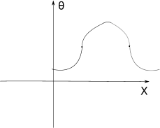
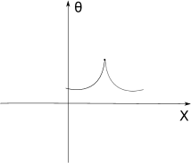
Figure 2. The first picture illustrates a one-sided cusp proved in Theorem 1. The third picture illustrates a full cusp singularity.

We close this section with a remark on why the singularity is a cusp singularity.

Remark 4.1.

By (4.6), we know that the maximum initial value of $|R(x,0)|$ is of $O(\varepsilon)$ order. It is easy to get that $R$ will be bounded above in any $O(1)$ time by studying the Riccati equation $\eqref{RxSx}_{2}$ and using $c^{\prime}>0$ which can be proved similarly as (4.13) when $\varepsilon$ is small enough. Thus, at the point of blowup, one has

$$S=\theta_{t}-c\theta_{x}=\infty,\quad|R|=|\theta_{t}+c\theta_{x}|<\hbox{constant},$$

which imply that $\theta_{t}=\infty$ and $\theta_{x}=-\infty$. The singularity is typically one-sided cusp. For carefully designed initial data, two opposite one-sided cusps might occur at the same time and the same location to form a full cusp. See Figure 2.

Together with the energy decay for smooth solutions, we know that the singularity formed in finite time is a cusp singularity with derivatives $|\theta_{x}|$ and $|\theta_{t}|$ being infinity, but the $L^{2}$ norms of which are finite. Hence $\theta$ is Hölder continuous with exponent $1/2$. By the estimate on $v_{t}$ in Lemma 3.1 and $u_{x}=v_{t}-\theta_{x}$, we also know that $u(\cdot,t)$ is Hölder continuous with exponent $1/2$ before and at the blowup.

5. A semilinear system in characteristic coordinates

As commented in Section 1.3 on the approach for global existence result, we will rewrite system (2.13) into a semilinear system in characteristic coordinates.

For any smooth solution $(u(x,t),\theta(x,t))$ of (1.1), the equations of the characteristics are

$$\frac{dx^{\pm}(s)}{ds}=\pm c\bigl{(}\theta(x^{\pm}(s),s)\bigr{)},$$ (5.1)

where, at time $s$,

$$x^{\pm}(s)\equiv x^{\pm}(s;\,x,\,t)$$

denote the forward and backward characteristics passing through the point $(x,t)$, respectively. Using the variables

$$S:=\theta_{t}-c(\theta)\theta_{x},\quad R:=\theta_{t}+c(\theta)\theta_{x},$$

defined in (4.1), we introduce new coordinates $(X,Y)$ by

$$\begin{split}X\equiv X(x,t):=&\int_{1}^{x^{-}(0;\,x,\,t)}(1+R^{2}(x^{\prime},0))\,dx^{\prime},\\ Y\equiv Y(x,t):=&\int_{x^{+}(0;\,x,\,t)}^{1}(1+S^{2}(x^{\prime},0))\,dx^{\prime}.\end{split}$$ (5.2)

It is easy to check that $X$ and $Y$ are constants along backward and forward characteristic, respectively; that is,

$$X_{t}-c(\theta)X_{x}=0\quad{\textrm{and}}\quad Y_{t}+c(\theta)Y_{x}=0.$$ (5.3)

Here we use $1+R^{2}$ and $1+S^{2}$ as the integrands in (5.2) just for later convenience in assigning the boundary data. One could choose other nonzero integrable functions as the integrands. For any smooth function $f$, it follows from (5.2) that

$$\left\{\begin{array}[]{l}f_{t}+c(\theta)f_{x}=f_{X}\,(X_{t}+c(\theta)X_{x})+f_{Y}\,(Y_{t}+c(\theta)Y_{x})=2cX_{x}f_{X},\\ f_{t}-c(\theta)f_{x}=f_{X}\,(X_{t}-c(\theta)X_{x})+f_{Y}\,(Y_{t}-c(\theta)Y_{x})=-2cY_{x}f_{Y}.\end{array}\right.$$ (5.4)

In order to complete the system, we introduce several variables:

$$w=2\arctan R,\qquad z=2\arctan S,$$ (5.5)

and

$$p=\frac{1+R^{2}}{X_{x}},\qquad q=\frac{1+S^{2}}{-Y_{x}}.$$ (5.6)

Furthermore, set $f=x$ and $f=t$ in two equations in (5.4) to get

$$\left\{\begin{array}[]{rcl}\displaystyle c&=&2cX_{x}x_{X},\\ \\ \displaystyle-c&=&-2cY_{x}x_{Y},\end{array}\right.\quad\left\{\begin{array}[]{rcl}\displaystyle 1&=&2cX_{x}t_{X},\\ \\ \displaystyle 1&=&-2cY_{x}t_{Y}.\end{array}\right.$$ (5.7)

Using (5.5) and (5.6), it holds

$$\left\{\begin{array}[]{ll}\displaystyle x_{X}=\frac{1}{2X_{x}}=\frac{1+\cos w}{4}p,\\ \\ \displaystyle x_{Y}=\frac{1}{2Y_{x}}=-\frac{1+\cos z}{4}q,\end{array}\right.\qquad\left\{\begin{array}[]{ll}\displaystyle t_{X}=\frac{1}{2cX_{x}}=\frac{1+\cos w}{4c}p,\\ \\ \displaystyle t_{Y}=-\frac{1}{2cY_{x}}=\frac{1+\cos z}{4c}q.\end{array}\right.$$ (5.8)

Then system (2.13) can be written as follows.

$$\begin{split}\theta_{X}&=\frac{\sin w}{4c}p,\quad\theta_{Y}=\frac{\sin z}{4c}q,\\ z_{X}&=\frac{p}{4c}\Big{\{}\frac{c^{\prime}}{c}(\cos^{2}\frac{w}{2}-\cos^{2}\frac{z}{2})-\sin w\cos^{2}\frac{z}{2}-\sin z\cos^{2}\frac{w}{2}-4J\cos^{2}\frac{z}{2}\cos^{2}\frac{w}{2}\Big{\}},\\ w_{Y}&=\frac{q}{4c}\Big{\{}\frac{c^{\prime}}{c}(\cos^{2}\frac{z}{2}-\cos^{2}\frac{w}{2})-\sin w\cos^{2}\frac{z}{2}-\sin z\cos^{2}\frac{w}{2}-4J\cos^{2}\frac{z}{2}\cos^{2}\frac{w}{2}\Big{\}},\\ p_{Y}&=\frac{pq}{2c}\Big{\{}\frac{c^{\prime}}{4c}(\sin z-\sin w)-\frac{1}{4}\sin w\sin z-\sin^{2}\frac{w}{2}\cos^{2}\frac{z}{2}-J\sin w\cos^{2}\frac{z}{2}\Big{\}},\\ q_{X}&=\frac{pq}{2c}\Big{\{}\frac{c^{\prime}}{4c}(\sin w-\sin z)-\frac{1}{4}\sin w\sin z-\sin^{2}\frac{z}{2}\cos^{2}\frac{w}{2}-J\sin z\cos^{2}\frac{w}{2}\Big{\}}\end{split}$$ (5.9)

where, recalling that,

$$J=u_{x}+\theta_{t}=u_{x}+\frac{S+R}{2}.$$ (5.10)

A derivation of the semilinear system (5.9)-(5.10) is given in Appendix A.2. It is a special case of system (A.10) that is derived from (2.1).

Remark 5.1.

We observe that the new system is invariant under translation by $2\pi$ in $w$ and $z$. Actually, it would be more precise to work with the variables $\hat{w}=e^{iw}$ and $\hat{z}=e^{iz}$. However, for simplicity we shall use the variables $w$, $z$, keeping in mind that they range on the unit circle $[-\pi,\pi]$ with endpoints identified.

6. Global existence and energy decay

In this section, we prove the global existence and energy decay in Theorem 2. Here by global existence, we mean that, for any $T>0$, there exists a solution for $t\in[0,T]$.

We will work on system (2.13) and accomplish the proof of Theorem 2 in three steps. First, for any fixed $J$, we solve for $\theta=\theta^{J}$ of the wave equation $\eqref{simeqn}_{2}$ with $v_{t}$ replaced by $J$. Then, in the second step, substituting $\theta^{J}$ into $\eqref{simeqn}_{1}$ and solving for $v=v^{J}$, we obtain a map from $J$ to $\mathcal{M}(J):=v^{J}_{t}$, which is basically (3.15)-(3.16), and then show this map has a fixed point, for a small time interval. Finally, we prove the energy decay and extend the local existence result to a global one.

Since we will use the Schauder fixed point theorem, we cannot achieve uniqueness in this paper. As a consequence, the solutions obtained for $t\in[0,T_{1}]$ and for $t\in[0,T_{2}]$ with $T_{2}>T_{1}$ might not agree with each other for $t\in[0,T_{1}]$. Hence we cannot claim an existence result for $t\in[0,\infty)$. The uniqueness for the variational wave equation was proved in [3]. So this might be a very interesting technique issue which, hopefully, could be conquered later, although the method in this paper fails to give a uniqueness.

6.1. Existence result for the wave equation with any given $J$

In this subsection, we first prove the existence of a weak solution for

$$\theta_{tt}+\theta_{t}=c(\theta)(c(\theta)\theta_{x})_{x}-J(x,t)$$ (6.1)

where $J(x,t)$ is given for any $(x,t)\in\mathbb{R}\times\mathbb{R}^{+}$, with

$$\|J\|_{C^{\alpha}\cap L^{\infty}\cap L^{2}(\Omega_{T})}=:\bar{J}(T)<\infty,$$ (6.2)

where

$$\Omega_{T}=\{(x,t)\,|\,x\in\mathbb{R},\;t\in[0,T]\}$$

for any $T\geq 0$. We fix an arbitrary time $T>0$, and only prove the existence of solution in $t\in[0,T]$. The equation (6.1) comes from $\eqref{simeqn}_{2}$ with $v_{t}$ replaced by $J$.

In the rest of paper, we always assume that $\alpha$ is a constant such that

$$0<\alpha<\frac{1}{4}.$$

By the initial condition (1.3), there exist $x_{a}$ and $x_{b}$, such that, $\theta_{1}(x)$, $\theta^{\prime}_{0}(x)$ and $J(x,0)=u^{\prime}_{0}(x)+\theta_{1}(x)$ are small enough for $x\not\in(x_{a},x_{b})$, particularly, if $\Omega^{a}$ and $\Omega^{b}$ are domains of dependence with bases $(-\infty,x_{a}]$ and $[x_{b},\infty)$, respectively, then solutions over $\Omega^{a}$ and $\Omega^{b}$ will not blow up before time $T$.

In fact, because $J$ is in $C^{\alpha}\cap L^{2}\cap L^{\infty}$ with $J(\pm\infty,0)=0$, for any $\varepsilon>0$, when $x_{a}$ and $x_{b}$ have sufficiently large magnitudes, $|J(x,t)|<\varepsilon$ for any $x<x_{a}$ or $x>x_{b}$ and $0\leq t\leq T$. Hence, one can find a priori bounds on gradient variables $R$ and $S$ using equations (4.3)-(4.4) and the initial smallness of $R$ and $S$. The existence and uniqueness for $C^{1}$ solutions in domains of dependence $\Omega^{a}$ and $\Omega^{b}$ is a classical result (see [29, 30] together with equations (4.3)-(4.4)). One can also use the semilinear equation method to find this unique solution. Note, when $T$ increases, $|x_{a}|$ and $|x_{b}|$ may increase.

The solution of (6.1) has a finite speed of propagation, so we can split the region $\Omega_{T}$ into different domains of dependence. As described in Figure 3 and its caption, now we only have to consider a characteristic triangle $\Omega^{0}$, which, together with $\Omega^{a}$ and $\Omega^{b}$, covers $\Omega_{T}$.

Due to the assumption (1.4) that the wave speed $c$ has positive lower and upper bounds, a time $T_{0}$, whose definition is clear from Figure 3, is finite.

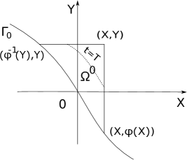
Figure 3. Left: $\Omega^{a}$ and $\Omega^{b}$ are domains of dependence corresponding to $x<x_{a}$ and $x>x_{b}$, respectively. When $-x_{a}$ and $x_{b}$ are sufficiently large, there will be no gradient blowup in $\Omega^{a}$ and $\Omega^{b}$ before $t=T$. $\Omega^{0}$ is another characteristic triangle, which covers $\Omega_{T}$ together with $\Omega^{a}$ and $\Omega^{b}$. Right: region $\Omega^{0}$ on the $(X,Y)$-plane.

6.1.1. Setup of the boundary value problem over $\Omega^{0}$ in the $(X,Y)$-coordinates.

Now we only have to consider the region $\Omega^{0}$ in Figure 3.

The key idea is to first construct the solution of semilinear system (5.9) then change it back to the original system. This idea was used for the variational wave equation in [6]. The appearance of the source term $J$ in our equation makes the existence proof harder than that in [6]. In fact, we do not have uniform a priori estimates for $p$ and $q$ by directly using the semi-linear system (5.9) in the $(X,Y)$-plane. Instead, we first establish the local existence for solutions in the $(X,Y)$-coordinates then transform it to the $(x,t)$-coordinates. Next, we will prove the key Lemma 6.2, in which the $L^{\infty}$ estimates for $p$ and $q$ are given. This helps extend the solution to $t\in[0,T]$.

Now we start from the boundary value problem on $\Omega^{0}$ in the $(X,Y)$-plane. The system for this boundary value problem is given in (6.1) with $J(x,t)$ given and satisfying (6.2).

The initial line $t=0$ in the $(x,t)$-plane is transformed to a parametric curve

$$\Gamma_{0}:=\big{\{}(X,Y):\,~{}~{}Y=\varphi(X)\big{\}}\subset{\mathbb{R}}^{2}$$ (6.3)

in the $(X,Y)$-plane, where $Y=\varphi(X)$ if and only if there is $x$ such that

$$X=\displaystyle\int_{0}^{x}[1+R^{2}(y,0)]\,dy\;\mbox{ and }\;Y=\displaystyle\int_{x}^{0}[1+S^{2}(y,0)]\,dy.$$ (6.4)

The curve $\Gamma_{0}$ is non-characteristic. The two functions $X=X(x),Y=Y(x)$ are well-defined and absolutely continuous. So $\varphi(X)$ is continuous and strictly decreasing in $X$ since $X(x)$ is strictly increasing while $Y(x)$ is strictly decreasing. From (1.2), (1.21) and (4.1), it follows

$$\big{|}X+\varphi(X)\big{|}\leq 4{\mathcal{E}}(0)<\infty\,.$$ (6.5)

As $(x,t)$ ranges over the domain $\Omega^{0}$, the corresponding variable $(X,Y)$ ranges over the set enclosed by one vertical line, one horizontal line and $\Gamma_{0}$, see Figure 3. Without loss of generality, we still use $\Omega^{0}$ to denote this region in the $(X,Y)$-plane.

Along the initial curve $\Gamma_{0}$ in (6.3) parametrized by $x\mapsto\big{(}X(x),\,Y(x)\big{)}$ using (6.4), we can thus assign the boundary data $\bar{\theta},\bar{z},\bar{w}$ $\in L^{\infty}$ by their definitions in (5.5) evaluated at the initial data, and $\bar{p}=1$ and $\bar{q}=1$ by (5.6), where we also used (1.2). Therefore, it is easy to check that

$$\int_{\Gamma_{0}}\frac{1-\cos\bar{w}}{4}\,dX-\frac{1-\cos\bar{z}}{4}\,dY\leq 2\mathcal{E}(0).$$

Finally, we denote

$$D=\hbox{Distance between two vertices of }\Omega^{0}\hbox{ on }\Gamma_{0}.$$ (6.6)

Since the wave speed $c$ has positive lower and upper bounds, clearly, $D$ is a constant depending only on the initial condition.

6.1.2. Local existence of the boundary value problem in $(X,Y)$ coordinates.

Now we first show a local existence result, by finding a fixed point of the map

$$(\hat{\theta},\hat{w},\hat{z},\hat{p},\hat{q})=\mathcal{T}_{1}(\theta,w,z,p,q)$$

defined by the solution of (5.9), more precisely,

$$\hat{\theta}(X,Y)=\theta(X,\phi(X))+\int_{\phi(X)}^{Y}\frac{\sin z}{4c}q(X,\bar{Y})d\bar{Y},$$ (6.7)

$$\begin{split}\hat{z}(X,Y)=&z(\phi^{-1}(Y),Y)+\int_{\phi^{-1}(Y)}^{X}p\Big{\{}\frac{c^{\prime}}{4c^{2}}(\cos^{2}\frac{w}{2}-\cos^{2}\frac{z}{2})\\ &-\frac{1}{4c}(\sin w\cos^{2}\frac{z}{2}+\sin z\cos^{2}\frac{w}{2})-\frac{1}{c}J(x_{p},t_{p})\cos^{2}\frac{z}{2}\cos^{2}\frac{w}{2}\Big{\}}(\bar{X},Y)d\bar{X},\end{split}$$ (6.8)

$$\begin{split}\hat{w}(X,Y)=&w(X,\phi(X))+\int_{\phi(X)}^{Y}q\Big{\{}\frac{c^{\prime}}{4c^{2}}(\cos^{2}\frac{z}{2}-\cos^{2}\frac{w}{2})\\ &-\frac{1}{4c}(\sin w\cos^{2}\frac{z}{2}+\sin z\cos^{2}\frac{w}{2})-\frac{1}{c}J(x_{m},t_{m})\cos^{2}\frac{z}{2}\cos^{2}\frac{w}{2}\Big{\}}(X,\bar{Y})d\bar{Y},\end{split}$$ (6.9)

$$\begin{split}\hat{p}(X,Y)=&p(X,\phi(X))+\int_{\phi(X)}^{Y}pq\left\{\frac{c^{\prime}}{8c^{2}}(\sin z-\sin w)\right.\\ &\left.-\frac{1}{2c}[\frac{1}{4}\sin w\sin z+\sin^{2}\frac{w}{2}\cos^{2}\frac{z}{2}]-\frac{1}{2c}J(x_{m},t_{m})\sin w\cos^{2}\frac{z}{2}\right\}(X,\bar{Y})d\bar{Y},\end{split}$$ (6.10)

$$\begin{split}\hat{q}(X,Y)=&q(\phi^{-1}(Y),Y)+\int_{\phi^{-1}(Y)}^{X}pq\left\{\frac{c^{\prime}}{8c^{2}}(\sin w-\sin z)\right.\\ &\left.-\frac{1}{2c}[\frac{1}{4}\sin w\sin z+\sin^{2}\frac{z}{2}\cos^{2}\frac{w}{2}]-\frac{1}{2c}J(x_{p},t_{p})\sin z\cos^{2}\frac{w}{2}\right\}(\bar{X},Y)d\bar{X},\end{split}$$ (6.11)

where

$$x_{p}(\bar{X},Y)=x(\bar{X},\phi(\bar{X}))+\int_{\phi(\bar{X})}^{Y}-\frac{1+\cos z}{4}qd\tilde{Y},$$ (6.12)

$$t_{p}(\bar{X},Y)=t(\bar{X},\phi(\bar{X}))+\int_{\phi(\bar{X})}^{Y}\frac{1+\cos z}{4c}qd\tilde{Y},$$ (6.13)

$$x_{m}(X,\bar{Y})=x(\phi^{-1}(\bar{Y}),\bar{Y})+\int_{\phi^{-1}(\bar{Y})}^{X}-\frac{1+\cos w}{4}pd\tilde{X},$$ (6.14)

and

$$t_{m}(X,\bar{Y})=t(\phi^{-1}(\bar{Y}),\bar{Y})+\int_{\phi^{-1}(\bar{Y})}^{X}-\frac{1+\cos w}{4c}pd\tilde{X}.$$ (6.15)

Note that $(x_{p},t_{p})$ and $(x_{m},t_{m})$ come from different but equivalent equations in (5.8). More importantly, such a choice makes sure that $(x_{p},t_{p})(\bar{X},Y)$ and $(x_{m},t_{m})(X,\bar{Y})$ have finite partial derivative in $Y$ and $X$, respectively.

For brief, we set

$$V=(\theta,w,z,p,q)\quad\hbox{and}\quad\hat{V}=(\hat{\theta},\hat{w},\hat{z},\hat{p},\hat{q}),$$

and let

$$\bar{V}(X)=(\theta,w,z,p,q)(X,\phi(X))$$

denote the initial data.

Fix a constant $K_{1}$ large to be determined later on (say $K_{1}\gg 2\|\bar{V}(X)\|_{C^{\alpha}\cap L^{\infty}}$). Define the set

$$\mathcal{K}_{1}=\left\{V\,\big{|}\,\|V(X,Y)\|_{C^{\alpha}\cap L^{\infty}(\hat{\Omega}_{\delta})}\leq K_{1},\ \ V(X,\phi(X))=\bar{V}(X)\right\}$$ (6.16)

where $\delta>0$ is a constant and

$$\hat{\Omega}_{\delta}=\big{\{}(X,Y)\in\Omega^{0}:\;\mbox{dist}((X,Y),\Gamma_{0})\leq\delta\big{\}}.$$ (6.17)

Note that the space $\mathcal{K}_{1}$ is compact in $C^{0}(\hat{\Omega}_{\delta})$, where $\hat{\Omega}_{\delta}$ is a two dimensional bounded connected region. We will apply the Schauder Fixed-Point Theorem to show that, there exists $\delta>0$, such that, the map $\mathcal{T}_{1}$ has a fixed point in the set $\mathcal{K}_{1}$.

The proof is standard and we will check the conditions for the theorem briefly.

For any local solution, when $\delta$ is small enough, it is easy to find uniform a priori bounds on $p$ and $q$ by corresponding equations in (5.9). We omit details here because we will later give much stronger global a priori bounds on $p$ and $q$, which will allow us to extend the solution to a global one.

Since $\mathcal{K}_{1}$ is a compact set in $C^{0}(\hat{\Omega}_{\delta})$ space, it suffices to show that the map $\mathcal{T}_{1}$ is continuous under $C^{0}$ norm and maps $\mathcal{K}_{1}$ to itself.

It follows directly from (6.7)-(6.11) that the map $\mathcal{T}_{1}$ is continuous since $J(x,t)$ is continuous in $x$ and $t$, and that $\mathcal{T}_{1}(V)(X,\phi(X))=V(X,\phi(X))$. Now recall that $J(x,t)$ is Hölder continuous in $x$ and $t$, and $(x_{p},t_{p})(\bar{X},Y)$ and $(x_{m},t_{m})(X,\bar{Y})$ have finite partial derivatives with respect to $Y$ and $X$. By (6.7)-(6.11), if $\delta$ is small enough, $\mathcal{T}_{1}$ maps $\mathcal{K}_{1}$ to itself. For example, $\hat{p}_{Y}$ is bounded, so $\hat{p}$ is Lipschitz in the $Y$ direction. In the $X$ direction, the $C^{\alpha}$ norm of $\hat{p}$ is different from the $C^{\alpha}$ norm of $p(X,\phi(X))$ by $C\delta$ times $\|V\|_{C^{\alpha}\cap L^{\infty}}$ for some constant $C$, where we use $J(x_{m},t_{m})$ is Hölder in $(x_{m},t_{m})$, and $(x_{m},t_{m})$ is Lipschitz in the $X$ direction.

So, we claim that there is a fixed point for the map $\mathcal{T}_{1}$ in $\mathcal{K}_{1}$.

Note that $\delta$ depends on $K_{1}$ while $K_{1}$ can be determined by the a priori bound on $\|V(X,Y)\|_{C^{\alpha}\cap L^{\infty}(\Omega^{0})}$. Later, in Lemma 6.2, we provide the a priori bounds on $p$ and $q$ in $\Omega^{0}$, by the map ${\mathcal{T}}_{1}$, and then we can find the $C^{\alpha}$ bound on $V$ as we just discussed. Clearly, the $L^{\infty}$ bound on $V$ is finite. So $K_{1}$ will be given by a constant only depending on the initial data $\bar{V}$. As a consequence, $\delta$ is fixed with respect to $K_{1}$. This allows one to apply the same procedure to extend the solution to $\Omega^{0}$.

Remark 6.1.

The equations of $\theta_{X}$ and $\theta_{Y}$ are equivalent since it is easy to check that $\theta_{XY}=\theta_{YX}$, as in [6]. The semilinear system (5.9) are invariant under translation by $2\pi$ in $w$ and $z$. It would be more precise to work with the variables $e^{iw}$ and $e^{iz}$. For simplicity, we shall use the variables $w$ and $z$ keeping in mind that they range on the unit circle $[-\pi,\pi]$ with endpoints identified.

6.1.3. Inverse transformation

Now we can carry out the inverse transformation from the $(X,Y)$-coordinate to the $(x,t)$-coordinate. This step is very similar to the one in [6]. Let’s only briefly introduce the key steps for completeness.

For convenience, we recall (5.8) below

$$\left\{\begin{array}[]{ll}\displaystyle x_{X}=\frac{1}{2X_{x}}=\frac{1+\cos w}{4}p,\\ \\ \displaystyle x_{Y}=\frac{1}{2Y_{x}}=-\frac{1+\cos z}{4}q,\end{array}\right.\qquad\left\{\begin{array}[]{ll}\displaystyle t_{X}=\frac{1}{2cX_{x}}=\frac{1+\cos w}{4c}p,\\ \\ \displaystyle t_{Y}=-\frac{1}{2cY_{x}}=\frac{1+\cos z}{4c}q.\end{array}\right.$$ (6.18)

It is easy to check that

$$t_{XY}=t_{YX},\qquad x_{XY}=x_{YX}$$

using (6.18) and (5.9), so two $t$ equations and two $x$ equations in (6.18) are equivalent, respectively. Hence, by (6.12)-(6.15),

$$(x_{m},t_{m})=(x_{p},t_{p})=:(x,t)$$

And, (6.18) provides an inverse transformation from the $(X,Y)$-coordinates to the $(x,t)$-coordinates.

Next, we note that the map from $(X,Y)$ to $(x,t)$ may not be one-to-one, since $(t_{X},x_{X})$ and $(t_{Y},x_{Y})$ might vanish as singularity forms. But, if

$$x(X_{1},Y_{1})=x(X_{2},Y_{2}),\quad t(X_{1},Y_{1})=t(X_{2},Y_{2}),$$

then

$$\theta(x(X_{1},Y_{1}),t(X_{1},Y_{1}))=\theta(x(X_{2},Y_{2}),t(X_{2},Y_{2})),$$

and hence, the function $\theta(x,t)$ is well defined and

$$dx\,dt=\frac{pq}{2c(1+R^{2})(1+S^{2})}dX\,dY=\frac{pq}{2c}\cos^{2}\frac{w}{2}\cos^{2}\frac{z}{2}\,dX\,dY.$$ (6.19)

We omit the proof here and refer the readers to [6] for more details.

6.1.4. Global existence of (5.9)

Now we extend the local solution of (5.9) established in Section 6.1.2 to $\Omega_{T}$. As we discussed, we only need some global a priori bounds on $p$ and $q$, which will be given in the next key lemma.

Lemma 6.2.

Consider any solution of (5.9) constructed in the local existence result up to the region $\Omega^{0}$. Then, we have

$$0<A_{1}\leq\max_{(X,Y)\in\Omega^{0}}\left\{p(X,Y),\,q(X,Y)\right\}\leq A_{2},$$ (6.20)

for some constants $A_{1}$ and $A_{2}$ specified in the proof.

Proof.

Figure 4. The domain $\Sigma$.

We consider a characteristic triangle $\Sigma$ in $\Omega^{0}$ enclosed by the line segment between $(X,Y)$ and $(X,\varphi(X))$, the line segment between $(X,Y)$ and $(\varphi^{-1}(Y),Y)$, and $\Gamma_{0}$. See Figure 4. If we denote equations of $p$ and $q$ in (5.9) as

$$q_{X}=Apq,\quad p_{Y}=Bpq,$$

then $p$ and $q$ are positive since $p=q=1$ on $\Gamma_{0}$. Furthermore, direct computation using (5.9) gives

$$\begin{split}\int_{\partial\Sigma}p\,d\bar{X}-q\,d\bar{Y}=&-\iint_{\Sigma}q_{X}+p_{Y}\,d\bar{X}d\bar{Y}\\ =&\iint_{\Sigma}\frac{pq}{2c}(\sin\frac{w}{2}\cos\frac{z}{2}+\sin\frac{z}{2}\cos\frac{w}{2})^{2}\,d\bar{X}d\bar{Y}\\ &+\iint_{\Sigma}\frac{pq}{2c}J(\sin z\cos^{2}\frac{w}{2}+\sin w\cos^{2}\frac{z}{2})\,d\bar{X}d\bar{Y}.\end{split}$$

Thus, using $p=q=1$ on $\Gamma_{0}$ again,

$$\int_{\varphi^{-1}(Y)}^{X}p(\bar{X},Y)\,d\bar{X}+\int^{Y}_{\varphi(X)}q(X,\bar{Y})\,d\bar{Y}$$

$$\quad=X-\varphi^{-1}(Y)+Y-\varphi(X)-\iint_{\Sigma}\frac{pq}{2c}(\sin\frac{w}{2}\cos\frac{z}{2}+\sin\frac{z}{2}\cos\frac{w}{2})^{2}\,dXdY$$

$$\qquad-\iint_{\Sigma}\frac{pq}{2c}J(\sin z\cos^{2}\frac{w}{2}+\sin w\cos^{2}\frac{z}{2})\,dXdY$$ (6.21)

$$\quad=X-\varphi^{-1}(Y)+Y-\varphi(X)-\iint_{\Sigma}\frac{pq}{2c}(\tan\frac{w}{2}+\tan\frac{z}{2})^{2}\cos^{2}\frac{z}{2}\cos^{2}\frac{w}{2}\,dXdY$$

$$\qquad-\iint_{\Sigma}\frac{pq}{2c}2J(\tan\frac{w}{2}+\tan\frac{z}{2})\cos^{2}\frac{z}{2}\cos^{2}\frac{w}{2}\,dXdY$$

$$\quad\leq X-\varphi^{-1}(Y)+Y-\varphi(X)+\iint_{\Sigma}\frac{pq}{2c}|J|^{2}\cos^{2}\frac{z}{2}\cos^{2}\frac{w}{2}\,dXdY$$

$$\quad\leq X-\varphi^{-1}(Y)+Y-\varphi(X)+\iint_{\tilde{\Sigma}}|J|^{2}\,dxdt$$

$$\quad\leq 2D+\bar{J}(T)$$ (6.22)

where we use (6.2), (6.6) and (6.19) in the last step. The constant $\bar{J}(T)$ is defined in (6.2). Here $\tilde{\Sigma}$ denotes the characteristic triangle in the $(x,t)$ plane transformed from $\Sigma$.

It then follows from $p_{Y}=Bpq$ that

$$p(X,Y)\leq e^{\sup{|B|}\,\int_{\phi(X)}^{Y}q(X,Y^{\prime})\,dY^{\prime}}<e^{\sup{|B|}\,(2D+\bar{J}(T))},$$

where $\sup{|B|}$ also depending on $\bar{J}(T)$.

The other bounds in (6.20) can be found similarly. ∎

6.1.5. Global existence for the wave equation

Finally, we show that $\theta(x,t)$ is a weak solution for the wave equation (6.1) in the $(x,t)$-plane for $0\leq t\leq T$, i.e. on $\Omega_{T}$.

We can prove the local Hölder continuity of $\theta$ in both $x$ and $t$ with exponent $1/2$ by showing that the integrals of $(\theta_{t}+c(\theta)\theta_{x})^{2}$ and $(\theta_{t}-c(\theta)\theta_{x})^{2}$ along forward and backward characteristics, respectively, are bounded. Then using the Sobolev embedding from $H^{1}$ to $C^{1/2}$. Note we also use the property on wave speed $c$ in (1.4). This also shows that all characteristic curves are $C^{1}$ with Hölder continuous derivative. Finally, one can show that

$$\iint_{\Omega_{0}}\left(\theta_{t}\phi_{t}-(c(\theta)\phi)_{x}c(\theta)\theta_{x}-\theta_{t}\phi-J\phi\right)\,dxdt=0$$ (6.23)

for any test function $\phi$ on $\Omega^{0}$. Applying this on the overlap domain $\Omega^{a}\cap\Omega^{0}$ or $\Omega^{b}\cap\Omega^{0}$, and by the uniqueness of $C^{1}$ solution on $\Omega^{a}$ and $\Omega^{b}$, we can glue solutions found on three regions $\Omega^{a}$, $\Omega^{b}$ and $\Omega^{0}$ to get a solution $\theta(x,t)$ for (6.1), when $t\in[0,T]$, in the weak sense of

$$\int_{0}^{T}\int_{\mathbb{R}}\left(\theta_{t}\phi_{t}-(c(\theta)\phi)_{x}c(\theta)\theta_{x}-\theta_{t}\phi-J\phi\right)\,dxdt=0$$ (6.24)

for $\phi\in C_{0}^{\infty}\{(x,t)\in\mathbb{R}\times[0,T]\}$. Since the proofs of these results are very similar to those in [6], we refer the readers to [6] for details.

Finally, for this part, we will prove that

$$E(t)=\int_{-\infty}^{\infty}(\theta_{t}^{2}+c^{2}(\theta)\theta_{x}^{2})(x,t)dx<C_{E}$$ (6.25)

for a constant $C_{E}$ depending on $E(0)$ and $J$, where $E(t)$ is first given in (4.8).

For any $\tau\geq 0$, let $\Gamma_{\tau}\subset\Omega^{+}$ be the transformation of the horizontal line $t=\tau$ in the $(x,t)$-plane.

Figure 5. The domain $D_{t}$ is enclosed by four curves with vertices $A,B,C,D$.

We first consider the bounded domain $D_{t}$ in the $(X,Y)$-plane in Figure 5, where $D_{t}$ is enclosed by two curves $AB$ and $CD$ with

$$AB\subset\Gamma_{t}\cap\partial D_{t},\quad CD\subset\Gamma_{0}\cap\partial D_{t}$$ (6.26)

and two straight line-segments $BC$ and $DA$. Here we denote four vertices in $(x,t)$ coordinates as

$$A=(a,t),\quad B=(b,t),\quad C=(c,0),\quad D=(d,0)$$ (6.27)

for some $a<b$ and $d<c$, respectively.

By Green’s theorem,

$$\begin{split}&\int_{\partial D_{t}}\frac{1-\cos w}{4}p\,dX-\frac{1-\cos z}{4}q\,dY\\ &\qquad=-\frac{1}{4}\iint_{D_{t}}\big{[}((1-\cos z)q)_{X}+((1-\cos w)p)_{Y}\big{]}\,dXdY.\end{split}$$ (6.28)

Direct computation from (5.9) gives

$$\begin{split}&((1-\cos z)q)_{X}+((1-\cos w)p)_{Y}\\ &\quad=-\frac{pq}{c}(\sin\frac{w}{2}\cos\frac{z}{2}+\sin\frac{z}{2}\cos\frac{w}{2})^{2}-\frac{pq}{c}J(\sin z\cos^{2}\frac{w}{2}+\sin w\cos^{2}\frac{z}{2}).\end{split}$$ (6.29)

Substituting it into (6.28), and using the transformation relation in (5.8), the following inequality holds, where curves $AB$ and $DC$ have starting points $A$, $D$ and ending points $B$, $C$, respectively.

$$\begin{split}&\int_{a}^{b}(\theta_{t}^{2}+c^{2}(\theta)\theta_{x}^{2})(x,t)\,dx\\ &\quad=\int_{AB\cap(\cos w\neq-1)}\frac{1-\cos w}{4}p\,dX+\int_{BA\cap(\cos z\neq-1)}\frac{1-\cos z}{4}q\,dY\\ &\quad\leq\int_{AB}\frac{1-\cos w}{4}p\,dX-\frac{1-\cos z}{4}q\,dY\\ &\quad=\int_{DC}\frac{1-\cos w}{4}p\,dX-\frac{1-\cos z}{4}q\,dY-\int_{DA}\frac{1-\cos w}{4}p\,dX\\ &\qquad-\int_{CB}\frac{1-\cos z}{4}q\,dY-\frac{1}{4}\iint_{D_{t}}\frac{pq}{c}(\sin\frac{w}{2}\cos\frac{z}{2}+\sin\frac{z}{2}\cos\frac{w}{2})^{2}\,dXdY\\ &\qquad-\frac{1}{4}\iint_{D_{t}}\frac{pq}{c}J(\sin z\cos^{2}\frac{w}{2}+\sin w\cos^{2}\frac{z}{2})\,dXdY\\ &\quad\leq\int_{DC}\frac{1-\cos w}{4}p\,dX-\frac{1-\cos z}{4}q\,dY-2\iint_{\mathcal{D}}\theta^{2}_{t}\,dxdt-2\iint_{\mathcal{D}}J\theta_{t}\,dxdt\\ &\quad=\int_{d}^{c}(\theta_{t}^{2}+c^{2}(\theta)\theta_{x}^{2})(x,0)\,dx-2\iint_{\mathcal{D}}\theta^{2}_{t}\,dxdt-2\iint_{\mathcal{D}}J\theta_{t}\,dxdt,\end{split}$$ (6.30)

where we have used the following fact in the second last step:

$$\left|\frac{\partial(X,Y)}{\partial(x,t)}\right|=\left|\begin{array}[]{cc}\displaystyle X_{x}&\displaystyle X_{t}\\ \displaystyle Y_{x}&\displaystyle Y_{t}\end{array}\right|=-2cX_{x}Y_{x}=\frac{8}{pq}\frac{1}{1+\cos w}\frac{1}{1+\cos z},$$

and $\mathcal{D}$ is the region in the $(x,t)$-plane transformed from $D_{t}$. The last equal sign holds since there exists no energy concentration initially using $\theta_{0}(x)$ is absolutely continuous.

If we let $(a,b)$ goes to $(-\infty,\infty)$, then by (6.30) we have, for any $0\leq t\leq T$,

$$E(t)\leq E(0)+4\int_{0}^{t}\int_{-\infty}^{\infty}|J||\theta_{t}|\,dxdt,$$

and hence,

$$\frac{1}{2}\max_{0\leq t\leq T}E(t)\leq E(0)+4C_{\varepsilon}\int_{0}^{T}\int_{-\infty}^{\infty}|J|^{2}\,dxdt$$

for some constant $C_{\varepsilon}$ and $C$. This gives (6.25), and implies that $\theta_{t}(\cdot,t)$ and $\theta_{x}(\cdot,t)$ are both square integrable functions in $x$, so do $R$ and $S$.

In summarize, we have

Lemma 6.3.

Fix any $T>0$ and any function $J(x,t)$ satisfying (6.2) over $\Omega_{T}$. If the same assumptions on initial conditions in Theorem 2 hold, then there exists a weak solution of (6.1) over $\Omega_{T}$ with bounded energy $E(t)<C_{E}$ for some $C_{E}$ depending on $E(0)$ and $J$.

6.2. A map from $J(x,t)$ to $J(X,Y)$

Using similar method as in Lemmas 1 and 2 in [3] for variational wave equation (i.e. (6.1) with $J\equiv 0$), we can show that the uniqueness of forward and backward characteristics for equation (6.1), i.e. the uniqueness of the $(X,Y)$ coordinates. Hence $(x_{m}(X,Y),t_{m}(X,Y))=(x_{p}(X,Y),t_{p}(X,Y))$ is unique. As a consequence, for any given $J(x,t)\in C^{\alpha}\cap L^{2}\cap L^{\infty}$, solution we found previously satisfies the semilinear system (5.9) with a unique source term $\tilde{J}(X,Y)=J(x(X,Y),t(X,Y))$.

Clearly $\tilde{J}(X,Y)$ is $L^{\infty}$. In fact, for any given $\tilde{J}(X,Y)\in L^{\infty}$, the semilinear system (5.9) has a unique solution obtained as the fixed point of a contract mapping in a weighted $L^{\infty}$ space, in the same way as the proof in [2]. As a consequence, we know that the solution $(x,t,\theta,w,z,p,q)(X,Y)$ of the semilinear system (5.9) is continuously dependent on $J$ in the $L^{\infty}$ space, due to the uniform bounds on $p$ and $q$ and the relation (5.8). The proof is straightforward and we omit the detail.

Remark 6.4.

The main idea in [3] for the variational wave equation is to find some Lipschitz weighted distance between any two characteristics. This distance essentially measures the forward and backward energy between two characteristics. The Lipschitz property protects the uniqueness of characteristics. By adding $J(x,t)\in C^{\alpha}\cap L^{2}\cap L^{\infty}$, there will be some new lower order terms $-2SJ$ and $-2RJ$ in the energy balance laws (A.8). This will not cause any problem since $S,R,J$ are all in $L^{2}$. The appearance of damping term never makes trouble here. Since this uniqueness result can be shown in a very similar way as in [3], we omit the proof here.

Remark 6.5.

The $(X,Y)$-coordinates system is ideal for the wave equation but it is not the case for the heat equation. The original $(x,t)$-coordinates system works better for the heat equation. So we run our proof mainly in the $(x,t)$-coordinates system and use the continuous dependence of solution on $J$ in the $(X,Y)$-coordinates system.

From $J(x,t)$ to $\tilde{J}(X,Y)$, there is actually an unfolding process when singularity forms, i.e. when characteristics tangentially touch each other.

6.3. A fixed point argument for a map on $J$

Recall that, for any given function $J(x,t)\in(C^{\alpha}\cap L^{\infty}\cap L^{2})(\Omega_{T})$, there exists a weak solution $\theta(x,t)=\theta^{J}(x,t)$ of (6.1).

Using relations (3.16) and (3.15), we define a function $\mathcal{M}(J)$ on $\Omega_{T}$ as follows

$$\begin{split}\mathcal{M}(J)(x,t)=&\int_{\mathbb{R}}H(x-y,t)\left(u_{0}^{\prime}(y)+\theta_{1}(y)\right)\,dy\\ &+\int_{0}^{t}\int_{\mathbb{R}}H(x-y,t-s)\big{[}2\theta_{s}+c^{\prime}(\theta)c(\theta)(\theta_{y})^{2}\big{]}(y,s)\,dyds\\ &-\int_{0}^{t}\int_{\mathbb{R}}H_{y}(x-y,t-s)\big{[}c^{2}(\theta)\theta_{y}-u\big{]}(y,s)\,dyds\end{split}$$ (6.31)

for $t\in[0,T]$ and

$$\begin{split}u(x,t)=&\int_{\mathbb{R}}H(x-y,t)u_{0}(y)\,dy+\int_{0}^{t}\int_{\mathbb{R}}H_{x}(x-y,t-s)\theta_{s}(y,s)\,dyds.\end{split}$$ (6.32)

This gives a map

$$\mathcal{T}:\ J(x,t)\rightarrow\mathcal{M}(J)(x,t)$$ (6.33)

on $C^{\alpha}\cap L^{\infty}\cap L^{2}(\Omega_{T})$.

Initially, we define a set $\mathcal{K}$ as follows: for some constants $\delta$ and $K$,

$$\mathcal{K}=\left\{J(x,t)\,\big{|}\,\|J(x,t)-J^{0}(x,t)\|_{C^{\alpha}\cap L^{\infty}\cap L^{2}(\Omega_{\delta})}\leq K,\ J(x,0)=\theta_{1}(x)+u^{\prime}_{0}(x)\right\}$$ (6.34)

where

$$\begin{split}J^{0}(x,t)=\int_{\mathbb{R}}H(x-y,t)\left(u_{0}^{\prime}(y)+\theta_{1}(y)\right)\,dy\end{split}$$

and

$$\Omega_{\delta}=\{(x,t)\,|\,x\in\mathbb{R},\;t\in[0,\delta]\}.$$

The goal in this subsection is first to show, for a given large $K$, if $\delta$ is sufficiently small, then $\mathcal{T}$ has a fixed point on $\mathcal{K}$. In general, $\delta$ would depend on $K$. Later, after proving the energy estimate in Theorem 3, we will establish a uniform bound on ${\mathcal{E}}(t)$ and we will be able to choose $K$ as the a priori bound on $\|J(x,t)-J^{0}(x,t)\|_{C^{\alpha}\cap L^{\infty}\cap L^{2}(\Omega_{\delta})}$, which depends only on the initial data. As a consequence, $\delta>0$ can be fixed in terms of the initial data. Hence, one can extend the existence to $\Omega_{T}$ in finite step.

The existence of a fixed point for small $\delta$ will be accomplished in several steps.

(i).

As before, we consider the far field separately, where the solution of forced wave equation is smooth due to finite propagation.

At time $t=0$, $J(x,0)=\theta_{1}(x)+u^{\prime}_{0}(x)$ for any function $J$ in $\mathcal{K}$. Furthermore, all functions in $\mathcal{K}$ have uniform $C^{\alpha}$, $L^{\infty}$ and $L^{2}$ bounds. So by a very similar argument as in the beginning of Section 6.1, we can find a domain $\Omega^{0}$ as in Figure 3, such that for any function $J$, the corresponding $\theta^{J}$, solved by the forced wave equation, has no singularity in the region $\Omega_{T}/\Omega^{0}$. Note that the solution $\theta^{J}$ solved by the forced wave equation is finitely propagating.

The choose of $\Omega^{0}$ depends on both $T$ and $K$.

(ii).

To apply the Schauder Fixed-Point Theorem, we use the following Banach space $L^{*}$, which includes all functions $f$ in $\bigcap\limits_{p\in[2+\sigma,\infty)}L^{p}$ with a finite norm

$$\|f\|_{L^{*}(\Omega_{\delta})}=\sup\limits_{p\in[2+\sigma,\infty)}\|f\|_{L^{p}(\Omega_{\delta})}<\infty.$$

Here $\sigma$ is any given positive constant. It is easy to check that $L^{*}$ is a Banach space. Clearly, $\mathcal{K}\subset L^{*}$ and is bounded, since for any $f\in\mathcal{K}$,

$$\|f\|_{L^{p}}\leq\max(\|f\|_{L^{2}},\|f\|_{L^{\infty}})<K,\quad p\in[2+\sigma,\infty).$$ (6.35)

This can be easily proved by the Hölder inequality.

Claim: $\mathcal{K}$ is a compact set in $L^{*}$.

We divide the proof of the claim into two steps.

Step 1: We use Frechet-Kolmogorov theorem ([7, 37]) to prove that $\mathcal{K}$ is a compact subset of $L^{p}(\Omega_{\delta})$ for any $p\in[2+\sigma,\infty)$.

We can verify two conditions in Frechet-Kolmogorov theorem as following. For any $p\in[2+\sigma,\infty)$ and $f\in\mathcal{K}$,

$$\begin{split}&\Big{(}\int_{0}^{\delta}\int_{\mathbb{R}}|f(x+a,t+b)-f(x,t)|^{p}\,dxdt\Big{)}^{\frac{1}{p}}\\ &\leq\|f(x+a,t+b)-f(x,t)\|_{L^{\infty}}^{l}(\int_{0}^{\delta}\int_{\mathbb{R}}|f(x+a,t+b)-f(x,t)|^{p(1-l)}\,dxdt)^{\frac{1}{p}}\end{split}$$

where $p(1-l)>2$. Because $f$ has a uniformly bounded $C^{\alpha}\cap L^{\infty}\cap L^{2}$ norm, $\|f(x+a)-f(a)\|_{L^{p}(\Omega_{\delta})}$ uniformly approaches zero as $a\rightarrow 0$ in $\mathcal{K}$.

By the same argument as in paragraphs (i), for any $\epsilon$, there exists a constant $r_{0}>0$ such that, if $r>r_{0}$, then $J(x,t)$ is less than $\epsilon$ for any $x>r$, $0\leq t\leq\delta$. So

$$\int_{0}^{\delta}\int_{|x|>r}|f|^{p}\,dxdt\leq\epsilon^{pl}\,\int_{0}^{\delta}\int_{\mathbb{R}}|f|^{p(1-l)}\,dxdt\leq\epsilon^{pl}(\max\{\|f\|_{L^{2}},\|f\|_{L^{\infty}}\})^{p(1-l)},$$

with $p(1-l)>2$. This shows the uniform convergence of $\int_{0}^{\delta}\int_{|x|>r}|f|^{p}\,dxdt$ as $r$ goes to $\infty$.

It follows from Frechet-Kolmogorov theorem that $\mathcal{K}$ is a compact subset in $L^{p}(\Omega_{\delta})$ with $p\in[2+\sigma,\infty)$.

Step 2: We show that $\mathcal{K}$ is a compact subset in $L^{*}$.

In fact, for any bounded set in $\mathcal{K}$, we can find a convergent sequence $f_{n}^{1}$ in $L^{2+\sigma}$. Then in $f_{n}^{1}$, we can find a convergent sub-sequence $f_{n}^{2}$ converging in $L^{3}$, then until any $L^{n}$. Now we claim $f_{n}^{n}$ converges in $L^{*}$. Clearly, all sub-sequences converge to the same function $f^{*}$ in a.e. sense. Furthermore, since $f_{n}^{n}\in\mathcal{K}$, one has $\|f_{n}^{n}\|_{L^{p}}<K$ for $p\in[2+\sigma,\infty)$ by (6.35). Therefore, $\|f^{*}\|_{L^{p}}<K$ for $p\in[2+\sigma,\infty)$, and hence, $f^{*}\in L^{*}$ with $\|f^{*}\|_{L^{*}}<K$. The compactness proof is done, which completes the proof of the claim.

(iii).

To use the Schauder Fixed-Point Theorem for $\mathcal{T}$ on $\mathcal{K}$, we have to prove:

• The map $\mathcal{T}$ maps from $\mathcal{K}$ to itself, for a small time interval $(0,\delta)$.

• The map $\mathcal{T}$ is continuous under the $L^{*}$ norm.

Proof of (a). First we show that $\|\mathcal{M}(J)(X,Y)\|_{L^{\infty}\cap L^{2}(\Omega_{\delta})}<K$. In fact, it is easy to show that the super norm of $u$ defined in (6.32) is bounded. Then by the $L^{2}$ bound of $\theta_{t}$ in (6.25) and using a similar argument as in Lemma 3.1, we can show that

$$\|\mathcal{M}(J)(x,t)-J^{0}(x,t)\|_{L^{\infty}(\Omega_{\delta})}<{C\cdot\delta^{\frac{1}{4}}}<K$$

for $\delta$ small enough, where $C$ is a constant.

Now we treat the $L^{2}$ norm of $\mathcal{M}(J)$. By (6.32), it is easy to see that $u(x,t)$ is a weak solution of

$$u_{t}-u_{xx}=\theta_{tx}.$$ (6.36)

Similarly, by (6.31), $\mathcal{M}(J)(x,t)$ is a weak solution of

$${\mathcal{M}}_{t}-{\mathcal{M}}_{xx}=c(\theta)(c(\theta)\theta_{x})_{x}-u_{x}-2\theta_{t}$$ (6.37)

where the calculation is very similar to (3.4)-(3.8). Then by same arguments as in Lemma 3.1 and using (6.25), we know

$$\|\mathcal{M}(J)(x,t)-J^{0}(x,t)\|_{L^{2}(\Omega_{\delta})}<{C\cdot\delta^{\frac{1}{4}}}<K$$

if $\delta$ is small. Here, as before, we get use of the $t^{1/4}$ power in Lemma 3.1.

Finally, if $\delta$ is small, the estimate

$$\|\mathcal{M}(J)(x,t)-J^{0}(x,t)\|_{C^{\alpha}(\Omega_{\delta})}<{C\cdot\delta^{\frac{1}{4}-\alpha}}<K$$

when $\delta$ is small enough, can be derived directly from Lemma A.1 in Appendix A.3.

Proof of (b). First recall $(\theta,z,w,p,q,x,t)(X,Y)$ is Lipschitz continuously dependent on $\tilde{J}(X,Y)$ in the $L^{\infty}$ distance, as discussed in the previous section.

Note, all integrals in $\mathcal{M}$ can be written as “nice” equations using $\theta,z,w,p,q,x,t$ and (6.19). For example,

$$2\iint H(x-y,t-s)\theta_{s}(y,s)dyds=\iint\tilde{H}\,\frac{pq}{4c}(\sin{w}\cos^{2}\frac{z}{2}-\sin{z}\cos^{2}\frac{w}{2})\,dXdY,$$

where

$$\tilde{H}=H(x-y(X,Y),t-s(X,Y)).$$

So the continuity of $\mathcal{M}$ in super norm can be proved by the Lipschitz continuous dependence of $(\theta,z,w,p,q,x,t)(X,Y)$ on $J$ in the $L^{\infty}$ distance.

Clearly, the $L^{\infty}$ and $L^{*}$ norm are different in the whole domain, but they are the same in any bounded domain. Thanks to the finite propagation property for (6.1), we can split the region into $\Omega^{0}$ and the rest, where for any $J(x,t)\in\mathcal{K}$, singularity only happens on $\Omega^{0}$. The continuity of $\mathcal{M}(J)$ on $J$ is clear for smooth solutions on $\Omega/\Omega^{0}$. One can use both $L^{2}$ and $L^{\infty}$ norms estimate to cover the $L^{*}$ space. In $\Omega^{0}$, we know that

$$\|J_{2}-J_{1}\|_{L^{\infty}}=\lim_{p\rightarrow\infty}\|J_{2}-J_{1}\|_{L^{p}}\leq\|J_{2}-J_{1}\|_{L^{*}}.$$

Hence, we proved (b).

Therefore, by (a) and (b), an application of the Schauder Fixed-Point Theorem gives a fixed point $J^{*}(x,t)\in\mathcal{K}$ of $\mathcal{T}$, that is,

$$\mathcal{M}(J^{*})(x,t)=J^{*}(x,t).$$ (6.38)

Finally, let’s fix $J=J^{*}$ in (6.38). Then for any $0\leq t\leq\delta$, by previous results, we know that,

$$\theta_{t}(\cdot,t),\ \theta_{x}(\cdot,t)\in L^{2}(\mathbb{R})\;\mbox{ and }\;u,\,J\in L^{\infty}\cap L^{2}(\mathbb{R}\times[0,\delta]),\qquad$$ (6.39)

and by applying standard heat equation theory to (6.36),

$$u\in L^{2}([0,\delta],H^{1}(\mathbb{R})),\quad u_{t}\in L^{2}([0,\delta],H^{-1}(\mathbb{R})).$$

Furthermore, from

$$v=\int_{-\infty}^{x}u\,dz,$$

one has

$$v_{t}-v_{xx}=\theta_{t},$$

in the $L^{2}$ sense by (6.36), which means for any test function $\phi\in C_{0}^{\infty}(\mathbb{R}\times[0,\delta])$,

$$\iint v_{t}\phi\,dxdt=\iint(v_{xx}+\theta_{t})\phi\,dxdt=\iint(u_{x}+\theta_{t})\phi\,dxdt,$$ (6.40)

where this and also the following integrals are all on $\mathbb{R}\times[0,\delta]$. By (6.24), we also know that

$$\iint\theta_{t}\phi_{t}dxdt=\iint\left((c(\theta)\phi)_{x}c(\theta)\theta_{x}+\theta_{t}\phi+J\phi\right)\,dxdt.$$ (6.41)

Now we are ready to show that

$$J=v_{t},\quad a.e..$$

First notice that for any test function $\phi\in C_{0}^{\infty}(\mathbb{R}\times[0,\delta])$, there exist a function $\psi\in C_{0}^{\infty}(\mathbb{R}\times[0,\delta])$ such that

$$\psi_{t}+\psi_{xx}+\psi=\phi.$$ (6.42)

In fact, $\psi$ can be found by first solving (6.42) with an initial boundary value problem with zero boundary conditions on some bounded interval containing the support of $\phi$, then doing an zero extension. By (6.40) and (6.41),

$$\iint v_{t}\psi_{t}\,dxdt=\iint(v_{xx}+\theta_{t})\psi_{t}\,dxdt$$

and

$$\iint\theta_{t}\psi_{t}dxdt=\iint\left((c(\theta)\psi)_{x}c(\theta)\theta_{x}+\theta_{t}\psi+J\psi\right)\,dxdt.$$

Add above two equations up to get

$$\iint v_{t}(\psi_{t}+\psi_{xx})\,dxdt=\iint\left((c(\theta)\psi)_{x}c(\theta)\theta_{x}+\theta_{t}\psi+J\psi\right)\,dxdt.$$

Furthermore, by (6.37) we mean that

$$\iint J(\psi_{t}+\psi_{xx})\,dxdt=\iint\left((c(\theta)\psi)_{x}c(\theta)\theta_{x}+u_{x}\psi+2\theta_{t}\psi\right)\,dxdt.$$

Now comparing the above two equations, and using (6.40) and (6.42), we have

$$\iint(J-v_{t})\phi\,dxdt=0,$$ (6.43)

which shows that $J=v_{t}$, a.e., and

$$\iint J\phi\,dxdt=\iint(u_{x}+\theta_{t})\phi\,dxdt,$$ (6.44)

The equation (1.19) is satisfied due to (6.41) and (6.43).

Finally, it follows from (6.44), (6.39) and (6.25) that

$$u_{x}(x,t)\in L^{\infty}([0,\delta],L^{2}_{loc}(\mathbb{R})).$$

The Hölder continuous properties of $u$ and $\theta$ in Theorem 2 can be easily shown by the Sobolev embedding from $H^{1}_{loc}$ to $C^{1/2}$ in one space dimension.

6.4. Energy Estimate

We now prove the energy estimate for the weak solution established in Section 6.3, which provides the energy estimate in Theorem 2 and allows an extension of the solution to $[0,T]$.

Theorem 3.

Fix $T>0$. For any weak solution of system (1.1) constructed in Section 6.3, one has, for $t\in[0,T]$,

$$\mathcal{E}(t)\leq\mathcal{E}(0)-\iint_{\mathbb{R}\times[0,t]}(v_{t}^{2}+\theta^{2}_{t})\,dxdt.$$ (6.45)

Proof.

We first consider the bounded domain $D_{t}$ in the $(X,Y)$-plane in Figure 5, and using the corresponding notation (6.26)-(6.27). Recall that $\mathcal{D}$ is the region in the $(x,t)$-plane transformed from $D_{t}$.

We start our proof from inequality (6.30), where $J$ in the last integral can be replaced by $v_{t}$, that is,

$$\begin{split}\int_{a}^{b}(\theta_{t}^{2}+c^{2}(\theta)\theta_{x}^{2})(x,t)\,dx\leq&\int_{d}^{c}(\theta_{t}^{2}+c^{2}(\theta)\theta_{x}^{2})(x,0)\,dx\\ &-2\iint_{\mathcal{D}}\theta^{2}_{t}\,dxdt-2\iint_{\mathcal{D}}v_{t}\theta_{t}\,dxdt.\end{split}$$ (6.46)

By (6.44) and the discussion in Section 6.3, we know $J=v_{t}=v_{xx}+\theta_{t}$ holds true in the $L^{2}(\mathbb{R}\times[0,T])$ sense. Thus,

$$\begin{split}\iint_{\mathcal{D}}v_{t}\theta_{t}\,dxdt=\iint_{\mathcal{D}}(v_{t}^{2}-v_{xx}v_{t})\,dxdt,\end{split}$$ (6.47)

where $v_{xx}$, $\theta_{t}$, $v_{t}\in L^{2}(\mathcal{D})$. Integrating by parts, the second term becomes

$$\begin{split}-\iint_{\mathcal{D}}v_{xx}v_{t}\,dxdt=&\iint_{\mathcal{D}}v_{x}v_{xt}\,dxdt+\int_{AD}\frac{v_{x}v_{t}}{\sqrt{1+c^{2}}}\,ds-\int_{CB}\frac{v_{x}v_{t}}{\sqrt{1+c^{2}}}\,ds\\ =&\frac{1}{2}\int_{a}^{b}|v_{x}|^{2}(x,t)\,dx-\frac{1}{2}\int_{d}^{c}|v_{x}|^{2}(x,0)\,dx\\ &-\int_{0}^{t}(v_{t}v_{x})(x^{+}(t),t)\,dt-\int_{0}^{t}(v_{t}v_{x})(x^{-}(t),t)\,dt\end{split}$$ (6.48)

where $x^{+}(t)$ and $x^{-}(t)$ are characteristic $DA$ and $CB$ respectively. Substitute this identity into (6.47) to get

$$\begin{split}\iint_{\mathcal{D}}v_{t}\theta_{t}\,dxdt=&\iint_{\mathcal{D}}v_{t}^{2}\,dxdt+\frac{1}{2}\int_{a}^{b}u^{2}(x,t)\,dx-\frac{1}{2}\int_{d}^{c}u^{2}(x,0)\,dx\\ &-\int_{0}^{t}(v_{t}v_{x})(x^{+}(t),t)\,dt-\int_{0}^{t}(v_{t}v_{x})(x^{-}(t),t)\,dt.\end{split}$$ (6.49)

Because $v_{t}$ is uniformly bounded and $v_{x}=u\in L^{2}$,

$$-\int_{0}^{t}(v_{t}v_{x})(x^{+}(t),t)\,dt-\int_{0}^{t}(v_{t}v_{x})(x^{-}(t),t)\,dt\to 0\;\mbox{ as }\;(a,b)\rightarrow(-\infty,\infty).$$

Taking $(a,b)\to(-\infty,\infty)$ (so $(d,c)\to(-\infty,\infty)$ too) in (6.46) and (6.49), we have

$$\begin{split}\mathcal{E}(t)\leq\mathcal{E}(0)-\iint_{\mathbb{R}\times[0,t]}(v_{t}^{2}+\theta^{2}_{t})\,dxdt.\end{split}$$ (6.50)

This completes the proof. ∎

By Lemma 3.1, we know that the time step $\delta$ only depends on the bound of $\mathcal{E}(t)$ in (6.25). The previous theorem gives an a priori bound on $\mathcal{E}(t)$, which only depends on the initial condition. By this piece of information, we know $\delta$ is uniformly positive, so one can obtain a solution on $[0,T]$ in finite many time steps. Alternatively, one can choose $K$ larger than the a priori bound on $\|J(x,t)-J^{0}(x,t)\|_{C^{\alpha}\cap L^{\infty}\cap L^{2}(\Omega_{T})}$ only depending on the initial data, then directly find the fixed point for $t\in[0,T]$. Here there seems to be repetition in our presentation from local to global existence. We feel this might be helpful for the readers to understand the ideas for this involved proof. This completes the proof of Theorem 2.

Remark 6.6.

If the solution has no energy concentration at time $t_{1}$, i.e. $\cos w$ and $\cos z$ are not $-1$ or equivalently $\theta_{t}$ and $\theta_{x}$ both have no blowup at $t_{1}$, then for any $t_{2}\geq t_{1}$,

$$\mathcal{E}(t_{2})\leq\mathcal{E}(t_{1})-\int_{t_{1}}^{t_{2}}\int_{\mathbb{R}}(v_{t}^{2}+\theta^{2}_{t})\,dxdt.$$ (6.51)

In fact, one can still prove it using the same method in the last theorem.

However, if solution has energy concentration at time $t_{1}$, (6.51) might not be true, because some energy might be later released from concentration. In this case, one cannot get the last step of (6.30), where

$$\begin{split}\int_{DC}\frac{1-\cos w}{4}p&\,dX-\frac{1-\cos z}{4}q\,dY\\ >&\int_{DC\cap(\cos w\neq-1)}\frac{1-\cos w}{4}p\,dX+\int_{CD\cap(\cos z\neq-1)}\frac{1-\cos z}{4}q\,dY\\ =&\int_{d}^{c}\frac{1}{2}(\theta_{t}^{2}+c^{2}(\theta)\theta_{x}^{2})(x,t_{1})\,dx,\end{split}$$

with $DC$ on the curve $t=t_{1}$.

Appendix A

A.1. Derivation of system (2.1)

We consider the following form of solutions to the system (1.10)

$${\bf u}(x,t)=(0,0,u(x,t))^{T}\;\mbox{ and }\;{\bf n}(x,t)=\big{(}\sin\theta(x,t),0,\cos\theta(x,t)\big{)}^{T}.$$

It is easy to see that $\nabla\cdot{\bf u}(x,t)=0$, and ${\bf u}\cdot\nabla{\bf u}={\bf u}\cdot\nabla{\bf n}={\bf u}\cdot\nabla\dot{{\bf n}}=0$. Direct computation implies

$$D=\frac{1}{2}(\nabla{\bf u}+\nabla^{T}{\bf u})=\frac{1}{2}\left[\begin{array}[]{ccc}0&0&u_{x}\\ 0&0&0\\ u_{x}&0&0\end{array}\right],$$

$$\omega=\frac{1}{2}(\nabla{\bf u}-\nabla^{T}{\bf u})=\frac{1}{2}\left[\begin{array}[]{ccc}0&0&-u_{x}\\ 0&0&0\\ u_{x}&0&0\end{array}\right],$$

$${\bf n}\otimes{\bf n}=\left[\begin{array}[]{ccc}\sin^{2}\theta&0&\sin\theta\cos\theta\\ 0&0&0\\ \sin\theta\cos\theta&0&\cos^{2}\theta\end{array}\right].$$

Then

$$N=\dot{{\bf n}}-\omega{\bf n}=\left(\theta_{t}+\frac{1}{2}u_{x}\right)\big{(}\cos\theta,0,-\sin\theta\big{)}^{T},$$

$$N\otimes{\bf n}=\left(\theta_{t}+\frac{1}{2}u_{x}\right)\left[\begin{array}[]{ccc}\sin\theta\cos\theta&0&\cos^{2}\theta\\ 0&0&0\\ -\sin^{2}\theta&0&-\sin\theta\cos\theta\end{array}\right],$$

$${\bf n}\otimes N=\left(\theta_{t}+\frac{1}{2}u_{x}\right)\left[\begin{array}[]{ccc}\sin\theta\cos\theta&0&-\sin^{2}\theta\\ 0&0&0\\ \cos^{2}\theta&0&-\sin\theta\cos\theta\end{array}\right].$$

And also

$$D{\bf n}=\frac{1}{2}u_{x}\big{(}\cos\theta,0,\sin\theta\big{)}^{T},$$

$${\bf n}^{T}D{\bf n}=u_{x}\cos\theta\sin\theta,$$

$$D{\bf n}\otimes{\bf n}=\frac{1}{2}u_{x}\left[\begin{array}[]{ccc}\sin\theta\cos\theta&0&\cos^{2}\theta\\ 0&0&0\\ \sin^{2}\theta&0&\sin\theta\cos\theta\end{array}\right],$$

$${\bf n}\otimes D{\bf n}=\frac{1}{2}u_{x}\left[\begin{array}[]{ccc}\sin\theta\cos\theta&0&\sin^{2}\theta\\ 0&0&0\\ \cos^{2}\theta&0&\sin\theta\cos\theta\end{array}\right].$$

Hence

$$\begin{split}{\bf g}=&\gamma_{1}N+\gamma_{2}D{\bf n}\\ =&\gamma_{1}\theta_{t}\big{(}\cos\theta,0,-\sin\theta\big{)}^{T}+\frac{1}{2}u_{x}\big{(}(\gamma_{1}+\gamma_{2})\cos\theta,0,(\gamma_{2}-\gamma_{1})\sin\theta\big{)}^{T}.\end{split}$$

Since the last term in Oseen-Frank energy density is null Lagrangian term, without loss of generalization, we only compute the first three terms. The Oseen-Frank energy density of this case will be

$$W({\bf n},\nabla{\bf n})=K_{1}({\bf n}^{1}_{x})^{2}+K_{3}\big{(}({\bf n}^{1}{\bf n}^{1}_{x})^{2}+({\bf n}^{1}{\bf n}^{3}_{x})^{2}\big{)}=\frac{1}{2}\theta^{2}_{x}\big{(}K_{1}\cos^{2}\theta+K_{3}\sin^{2}\theta\big{)},$$

where ${\bf n}^{i}$ is the $i$-th component of ${\bf n}$. Thus

$$\frac{\partial W}{\partial{\bf n}}=\big{(}K_{3}\theta_{x}^{2}\sin\theta,0,0\big{)}^{T},$$

$$\frac{\partial W}{\partial\nabla{\bf n}}=\left[\begin{array}[]{ccc}K_{1}\theta_{x}\cos\theta+K_{3}\theta_{x}\sin^{2}\theta\cos\theta&0&0\\ 0&0&0\\ -K_{3}\theta_{x}\sin^{3}\theta&0&0\end{array}\right].$$

The Lagrangian constant

$$\begin{split}\gamma=&\frac{\partial W}{\partial{\bf n}}\cdot{\bf n}+\gamma_{2}D{\bf n}\cdot{\bf n}-\nabla\cdot\left(\frac{\partial W}{\partial\nabla{\bf n}}\right)\cdot{\bf n}-|{\bf n}_{t}|^{2}\\ =&(K_{1}+2K_{3})\theta_{x}^{2}\sin^{2}\theta-K_{1}\theta_{xx}\sin\theta\cos\theta+\gamma_{2}u_{x}\sin\theta\cos\theta-|\theta_{t}|^{2}.\end{split}$$

We are ready to derive the system (2.1). We first work on the equation of $\theta$. By the third equation of (1.10), we have

$$\begin{split}{\bf n}_{tt}=&\theta_{tt}\big{(}\cos\theta,0,-\sin\theta\big{)}^{T}+|\theta_{t}|^{2}\big{(}-\sin\theta,0,-\cos\theta\big{)}^{T}\\ =&\gamma{\bf n}-\frac{\partial W}{\partial{\bf n}}-{\bf g}+\nabla\cdot\left(\frac{\partial W}{\partial\nabla{\bf n}}\right)\\ =&-|\theta_{t}|^{2}\big{(}\sin\theta,0,\cos\theta\big{)}^{T}-\gamma_{1}\theta_{t}\big{(}\cos\theta,0,-\sin\theta\big{)}^{T}+u_{x}{\mathbf{T}_{1}}+K_{1}\mathbf{T}_{2}+K_{3}\mathbf{T}_{3}.\end{split}$$

Then

$$\begin{split}(\theta_{tt}+\gamma_{1}\theta_{t})\big{(}\cos\theta,0,-\sin\theta\big{)}^{T}=u_{x}{\mathbf{T}_{1}}+K_{1}\mathbf{T}_{2}+K_{3}\mathbf{T}_{3}.\end{split}$$ (A.1)

Here the vector $\mathbf{T}_{1}$ is given by

$$\begin{split}\mathbf{T}_{1}=&\gamma_{2}\sin\theta\cos\theta\big{(}\sin\theta,0,\cos\theta\big{)}^{T}-\frac{1}{2}\big{(}(\gamma_{1}+\gamma_{2})\cos\theta,0,(\gamma_{2}-\gamma_{1})\sin\theta\big{)}^{T}\\ =&-\frac{\gamma_{1}}{2}\big{(}\cos\theta,0,-\sin\theta\big{)}^{T}+\frac{\gamma_{2}}{2}\big{(}2\sin^{2}\theta\cos\theta-\cos\theta,0,2\sin\theta\cos^{2}\theta-\sin\theta\big{)}^{T}\\ =&\left(-\frac{\gamma_{1}}{2}-\frac{\gamma_{2}}{2}\cos(2\theta)\right)\big{(}\cos\theta,0,-\sin\theta\big{)}^{T}.\end{split}$$ (A.2)

The nonzero components of vector $\mathbf{T}_{2}$ is given by

$$\mathbf{T}_{2}^{1}= \theta_{x}^{2}\sin^{3}\theta-\theta_{xx}\sin^{2}\theta\cos\theta+(\theta_{x}\cos\theta)_{x}$$

$$= -\sin^{2}\theta(\theta_{x}\cos\theta)_{x}+(\theta_{x}\cos\theta)_{x}=\cos^{2}\theta(\theta_{x}\cos\theta)_{x},$$

$$\mathbf{T}_{2}^{3}= \theta_{x}^{2}\sin^{2}\theta\cos\theta-\theta_{xx}\sin\theta\cos^{2}\theta=-\sin\theta\cos\theta(\theta_{x}\cos\theta)_{x}.$$

So the vector $\mathbf{T}_{2}$ is

$$\begin{split}\mathbf{T}_{2}=\cos\theta(\theta_{x}\cos\theta)_{x}\big{(}\cos\theta,0,-\sin\theta\big{)}^{T}.\end{split}$$ (A.3)

Similarly, the vector $\mathbf{T}_{3}$ is

$$\begin{split}\mathbf{T}_{3}=\sin\theta(\theta_{x}\sin\theta)_{x}\big{(}\cos\theta,0,-\sin\theta\big{)}^{T}.\end{split}$$ (A.4)

Plugging (A.2), (A.3) and (A.4) into (A.1), we obtain

$$\theta_{tt}+\gamma_{1}\theta_{t}=K_{1}\cos\theta(\theta_{x}\cos\theta)_{x}+K_{3}\sin\theta(\theta_{x}\sin\theta)_{x}+\left(-\frac{\gamma_{1}}{2}-\frac{\gamma_{2}}{2}\cos(2\theta)\right)u_{x},$$

which is exactly the second equation in (2.1).

For the equation of $u$, direct computation gives

$$\nabla\cdot\left(\frac{\partial W}{\partial\nabla{\bf n}}\otimes\nabla{\bf n}\right)=\big{(}(K_{1}\theta_{x}^{2}\cos^{2}\theta)_{x}+(K_{3}\theta_{x}^{2}\sin^{2}\theta)_{x},0,0\big{)}^{T}$$

and

$$\begin{split}\nabla\cdot\sigma=&\alpha_{1}\big{(}(u_{x}\sin^{3}\theta\cos\theta)_{x},0,(u_{x}\sin^{2}\theta\cos^{2}\theta)_{x}\big{)}^{T}\\ &+\alpha_{2}\left(\big{(}(\theta_{t}+\frac{1}{2}u_{x})\sin\theta\cos\theta\big{)}_{x},0,-\big{(}(\theta_{t}+\frac{1}{2}u_{x})\sin^{2}\theta\big{)}_{x}\right)^{T}\\ &+\alpha_{3}\left(\big{(}(\theta_{t}+\frac{1}{2}u_{x})\sin\theta\cos\theta\big{)}_{x},0,\big{(}(\theta_{t}+\frac{1}{2}u_{x})\cos^{2}\theta\big{)}_{x}\right)^{T}\\ &+\frac{\alpha_{4}}{2}\big{(}0,0,u_{xx}\big{)}^{T}+\frac{\alpha_{5}}{2}\big{(}(u_{x}\sin\theta\cos\theta)_{x},0,(u_{x}\sin^{2}\theta)_{x}\big{)}^{T}\\ &+\frac{\alpha_{6}}{2}\big{(}(u_{x}\sin\theta\cos\theta)_{x},0,(u_{x}\cos^{2}\theta)_{x}\big{)}^{T}.\end{split}$$

Therefore the first equation of system (1.10) can be written into following three equations

$$\begin{split}P_{x}=&K_{1}(\theta_{x}^{2}\cos^{2}\theta)_{x}+K_{3}(\theta_{x}^{2}\sin^{2}\theta)_{x}+\alpha_{1}(u_{x}\sin^{3}\theta\cos\theta)_{x}\\ &+\frac{1}{2}\left(\alpha_{2}+\alpha_{3}+\alpha_{5}+\alpha_{6}\right)(u_{x}\sin\theta\cos\theta)_{x}+(\alpha_{2}+\alpha_{3})\big{(}\theta_{t}\sin\theta\cos\theta\big{)}_{x},\end{split}$$ (A.5)

$$P_{y}=0,$$ (A.6)

$$\begin{split}u_{t}+P_{z}=&\frac{\alpha_{4}}{2}u_{xx}+\alpha_{1}(u_{x}\sin^{2}\theta\cos^{2}\theta)_{x}-\alpha_{2}\big{(}(\theta_{t}+\frac{1}{2}u_{x})\sin^{2}\theta\big{)}_{x}\\ &+\alpha_{3}\big{(}(\theta_{t}+\frac{1}{2}u_{x})\cos^{2}\theta\big{)}_{x}+\frac{\alpha_{5}}{2}(u_{x}\sin^{2}\theta)_{x}+\frac{\alpha_{6}}{2}(u_{x}\cos^{2}\theta)_{x}.\end{split}$$ (A.7)

By these equations, one can obtain that $P_{z}=a$ for some constant $a$. The right hand side of (A.7) can be rewritten as $(g(\theta)u_{x}+h(\theta)\theta_{t})_{x}$ where $g(\theta)$ and $h(\theta)$ is defined as (2.2). Therefore, we obtain the first equation of (2.1).

A.2. Derivation of system (5.9)

We will in fact derive the semilinear system in $XY$-coordinates for (2.1) with $\nu=\rho=1$ and $a=0$. Recall, from (5.5) and (5.6), that we have introduced

$$w=2\arctan R,\quad z=2\arctan S,\quad p=\frac{1+R^{2}}{X_{x}},\quad q=-\frac{1+S^{2}}{Y_{x}}.$$

It is easy to have that

$$R=\tan\frac{w}{2},\quad\frac{R}{1+R^{2}}=\frac{1}{2}\sin w,\quad\frac{1}{1+R^{2}}=\cos^{2}\frac{w}{2},$$

$$S=\tan\frac{z}{2},\quad\frac{S}{1+S^{2}}=\frac{1}{2}\sin z,\quad\frac{1}{1+S^{2}}=\cos^{2}\frac{z}{2}.$$

By (5.4) and (4.2), we have

$$\theta_{X}=\frac{\sin w}{4c}p,\quad\theta_{Y}=\frac{\sin z}{4c}q.$$

Denote

$$U=h(\theta)u_{x}.$$

By (4.2), we have

$$\left\{\begin{array}[]{rcl}(S^{2})_{t}+c(\theta)(S^{2})_{x}&=&\frac{c^{\prime}}{2c}(S^{3}-R^{2}S)-\gamma_{1}(RS+S^{2})-2SU,\\ (R^{2})_{t}-c(\theta)(R^{2})_{x}&=&\frac{c^{\prime}}{2c}(R^{3}-RS^{2})-\gamma_{1}(RS+R^{2})-2RU,\end{array}\right.$$ (A.8)

so

$$\left\{\begin{array}[]{rcl}(S^{2})_{X}&=&\frac{1}{2c}p\frac{1}{1+R^{2}}\Big{\{}\frac{c^{\prime}}{2c}(S^{3}-R^{2}S)-\gamma_{1}(RS+S^{2})-2SU\Big{\}},\\ (R^{2})_{Y}&=&\frac{1}{2c}q\frac{1}{1+S^{2}}\Big{\{}\frac{c^{\prime}}{2c}(R^{3}-RS^{2})-\gamma_{1}(RS+R^{2})-2RU\Big{\}}.\end{array}\right.$$ (A.9)

Hence,

$$\begin{split}z_{X}=&\textstyle\frac{1}{1+S^{2}}\frac{1}{S}(S^{2})_{X}\\ =&\textstyle\frac{1}{2c}p\frac{1}{(1+R^{2})(1+S^{2})}\Big{\{}\frac{c^{\prime}}{2c}(S^{2}-R^{2})-\gamma_{1}(R+S)-2U\Big{\}}\\ =&\textstyle p\Big{\{}\frac{c^{\prime}}{4c^{2}}(\cos^{2}\frac{w}{2}-\cos^{2}\frac{z}{2})-\frac{\gamma_{1}}{4c}(\sin w\cos^{2}\frac{z}{2}+\sin z\cos^{2}\frac{w}{2})-\frac{1}{c}\cos^{2}\frac{z}{2}\cos^{2}\frac{w}{2}U\Big{\}}.\end{split}$$

Similarly,

$$\textstyle w_{Y}=q\Big{\{}\frac{c^{\prime}}{4c^{2}}(\cos^{2}\frac{z}{2}-\cos^{2}\frac{w}{2})-\frac{\gamma_{1}}{4c}(\sin w\cos^{2}\frac{z}{2}+\sin z\cos^{2}\frac{w}{2})-\frac{1}{c}\cos^{2}\frac{z}{2}\cos^{2}\frac{w}{2}U\Big{\}}.$$

On the other hand, using $X_{t}-cX_{x}=0$, we have

$$X_{tx}-cX_{xx}=\frac{c^{\prime}}{2c}(R-S)X_{x}.$$

Then

$$p_{Y}= \textstyle\frac{1}{X_{x}}(R^{2})_{Y}-\frac{q\cos^{2}{\frac{w}{2}}}{2c}\frac{1+R^{2}}{X_{x}^{2}}(X_{xt}-cX_{xx})$$

$$= \textstyle\frac{pq}{2c}\frac{1}{(1+R^{2})(1+S^{2})}\Big{\{}\frac{c^{\prime}}{2c}(R^{3}-RS^{2})-\gamma_{1}(RS+R^{2})-2RU\Big{\}}-\frac{pq}{2c}\frac{c^{\prime}}{2c}\frac{R-S}{1+S^{2}}$$

$$= \textstyle\frac{pq}{2c}\frac{1}{(1+R^{2})(1+S^{2})}\Big{\{}\frac{c^{\prime}}{2c}(-R-RS^{2})-\gamma_{1}(RS+R^{2})-2RU\Big{\}}+\frac{pq}{2c}\frac{c^{\prime}}{2c}\frac{S}{1+S^{2}}$$

$$= \textstyle pq\frac{c^{\prime}}{8c^{2}}(\sin z-\sin w)-\gamma_{1}\frac{pq}{2c}[\frac{1}{4}\sin w\sin z+\sin^{2}\frac{w}{2}\cos^{2}\frac{z}{2}]-\frac{pq}{2c}U\sin w\cos^{2}\frac{z}{2}.$$

Similarly, we have

$$q_{X}=\textstyle pq\frac{c^{\prime}}{8c^{2}}(\sin w-\sin z)-\gamma_{1}\frac{pq}{2c}[\frac{1}{4}\sin w\sin z+\sin^{2}\frac{z}{2}\cos^{2}\frac{w}{2}]-\frac{pq}{2c}U\sin z\cos^{2}\frac{w}{2}.$$

In summary, we have the following system of equations.

$$\begin{split}\theta_{X}&\textstyle=\frac{\sin w}{4c}p,\qquad\theta_{Y}=\frac{\sin z}{4c}q\\ z_{X}&\textstyle=p\Big{\{}\frac{c^{\prime}}{4c^{2}}(\cos^{2}\frac{w}{2}-\cos^{2}\frac{z}{2})-\frac{\gamma_{1}}{4c}(\sin w\cos^{2}\frac{z}{2}+\sin z\cos^{2}\frac{w}{2})-\frac{1}{c}\cos^{2}\frac{z}{2}\cos^{2}\frac{w}{2}U\Big{\}}\\ w_{Y}&\textstyle=q\Big{\{}\frac{c^{\prime}}{4c^{2}}(\cos^{2}\frac{z}{2}-\cos^{2}\frac{w}{2})-\frac{\gamma_{1}}{4c}(\sin w\cos^{2}\frac{z}{2}+\sin z\cos^{2}\frac{w}{2})-\frac{1}{c}\cos^{2}\frac{z}{2}\cos^{2}\frac{w}{2}U\Big{\}}\\ p_{Y}&\textstyle=pq\frac{c^{\prime}}{8c^{2}}(\sin z-\sin w)-\gamma_{1}\frac{pq}{2c}[\frac{1}{4}\sin w\sin z+\sin^{2}\frac{w}{2}\cos^{2}\frac{z}{2}]-\frac{pq}{2c}U\sin w\cos^{2}\frac{z}{2}\\ q_{X}&\textstyle=pq\frac{c^{\prime}}{8c^{2}}(\sin w-\sin z)-\gamma_{1}\frac{pq}{2c}[\frac{1}{4}\sin w\sin z+\sin^{2}\frac{z}{2}\cos^{2}\frac{w}{2}]-\frac{pq}{2c}U\sin z\cos^{2}\frac{w}{2}\end{split}$$

where recall that $U=h(\theta)u_{x}.$

Denote $J=g(\theta)u_{x}+h(\theta)\theta_{t}$. Then

$$U=\frac{h(\theta)}{g(\theta)}(J-h(\theta)\theta_{t}).$$

In terms of the variable $J$, the above system is

$$\begin{split}&\theta_{X}=\frac{\sin w}{4c}p,\quad\theta_{Y}=\frac{\sin z}{4c}q\\ &\textstyle z_{X}=p\Big{\{}\frac{c^{\prime}}{4c^{2}}(\cos^{2}\frac{w}{2}-\cos^{2}\frac{z}{2})+\frac{\frac{h^{2}(\theta)}{g(\theta)}-\gamma_{1}}{4c}(\sin w\cos^{2}\frac{z}{2}+\sin z\cos^{2}\frac{w}{2})-\frac{h(\theta)}{cg(\theta)}J\cos^{2}\frac{z}{2}\cos^{2}\frac{w}{2}\Big{\}}\\ &\textstyle w_{Y}=q\Big{\{}\frac{c^{\prime}}{4c^{2}}(\cos^{2}\frac{z}{2}-\cos^{2}\frac{w}{2})+\frac{\frac{h^{2}(\theta)}{g(\theta)}-\gamma_{1}}{4c}(\sin w\cos^{2}\frac{z}{2}+\sin z\cos^{2}\frac{w}{2})-\frac{h(\theta)}{cg(\theta)}J\cos^{2}\frac{z}{2}\cos^{2}\frac{w}{2}\Big{\}}\\ &\textstyle p_{Y}=pq\Big{\{}\frac{c^{\prime}}{8c^{2}}(\sin z-\sin w)+\frac{\frac{h^{2}(\theta)}{g(\theta)}-\gamma_{1}}{2c}(\frac{1}{4}\sin w\sin z+\sin^{2}\frac{w}{2}\cos^{2}\frac{z}{2})-\frac{h(\theta)}{2cg(\theta)}J\sin w\cos^{2}\frac{z}{2}\Big{\}}\\ &\textstyle q_{X}=pq\Big{\{}\frac{c^{\prime}}{8c^{2}}(\sin w-\sin z)+\frac{\frac{h^{2}(\theta)}{g(\theta)}-\gamma_{1}}{2c}(\frac{1}{4}\sin w\sin z+\sin^{2}\frac{z}{2}\cos^{2}\frac{w}{2})-\frac{h(\theta)}{2cg(\theta)}J\sin z\cos^{2}\frac{w}{2}\Big{\}}\end{split}$$ (A.10)

where the coefficient $\frac{h^{2}(\theta)}{g(\theta)}-\gamma_{1}<0$ by (2.11).

For the special case where $\gamma_{1}=2$, $\gamma_{2}=0$ and $g(\theta)=h(\theta)=1$, system (A.10) reduces to system (5.9).

A.3. Hölder continuity of $\mathcal{M}(J)$ in §6.3

First, we consider three types of integrals in the definition of $J$ in (6.31),

$$L_{i}(x,t):=\int_{\mathbb{R}}H(x-y,t)f(y)\,dy$$

$$L_{ii}(x,t):=\int_{0}^{t}\int_{\mathbb{R}}H(x-y,t-s)g(y,s)\,dyds$$

$$L_{iii}(x,t):=\int_{0}^{t}\int_{\mathbb{R}}H_{x}(x-y,t-s)f(y,s)\,dyds.$$

We first prove the following lemma working generally.

Lemma A.1.

If $f(x,t)\in L^{\infty}([0,T],L^{2}(\mathbb{R}))$, $g(x,t)\in L^{\infty}([0,T],L^{1}(\mathbb{R}))$ or $g(x,t)\in L^{\infty}([0,T],L^{2}(\mathbb{R}))$ we have $L_{j}(x,t)$ is Hölder continuous w.r.t $x$ and $t$, for all $j=i,ii,iii$, with exponent $\beta\in(0,\frac{1}{4})$.

Proof.

We only provide the proof of Hölder continuity w.r.t $x$ for $L_{iii}$, the rest cases can be proved similarly. For any $x_{1}<x_{2}$, it is sufficient to show

$$\left|\int_{0}^{t}\int_{\mathbb{R}}\frac{H_{y}(x_{2}-y,t-s)-H_{y}(x_{1}-y,t-s)}{(x_{2}-x_{1})^{\beta}}f(y,s)dyds\right|\leq\hbox{Constant}\,\cdot\,t^{\frac{1}{4}-\frac{\beta}{2}},$$ (A.11)

for some $\beta\in(0,1)$. Since

$$H_{x}(x,t)=-\frac{1}{4\sqrt{\pi}}\frac{x}{t^{3/2}}\exp\left(-\frac{x^{2}}{4t}\right),$$

$$\begin{split}&H_{x}(x_{2}-y,t-s)-H_{x}(x_{1}-y,t-s)\\ &\quad=-\frac{1}{4\sqrt{\pi}}\frac{1}{(t-s)^{3/2}}\left\{(x_{2}-x_{1})\exp\left(-\frac{(x_{2}-y)^{2}}{4(t-s)}\right)\right.\\ &\qquad-\left.(x_{1}-y)\left[\exp\left(-\frac{(x_{2}-y)^{2}}{4(t-s)}\right)-\exp\left(-\frac{(x_{1}-y)^{2}}{4(t-s)}\right)\right]\right\}\\ &\quad:=I_{1}+I_{2}.\end{split}$$

The integral related to the first term $I_{1}$ can be estimated as follows

$$\begin{split}&\int_{0}^{t}\int_{\mathbb{R}}\frac{1}{(t-s)^{3/2}}(x_{2}-x_{1})^{1-\beta}\exp\left(-\frac{(x_{2}-y)^{2}}{4(t-s)}\right)|f(y,s)|\,dyds\\ \leq&C\int_{0}^{t}\int_{\mathbb{R}}\frac{1}{(t-s)^{3/2}}\left(|x_{2}-y|^{1-\beta}+|x_{1}-y|^{1-d}\right)\exp\left(-\frac{(x_{2}-y)^{2}}{4(t-s)}\right)|f(y,s)|\,dyds.\end{split}$$ (A.12)

By the same argument in (3.9), and choosing $0<\beta<\frac{1}{8}$, the first term in (A.12) should be controlled by

$$\int_{0}^{t}\int_{\mathbb{R}}\frac{1}{(t-s)^{3/2}}|x_{2}-y|^{1-\beta}\exp\left(-\frac{(x_{2}-y)^{2}}{4(t-s)}\right)|f(y,s)|\,dyds\leq Ct^{\frac{1}{4}-\frac{\beta}{2}}\|f\|_{L^{\infty}((0,T),L^{2}(\mathbb{R}))}.$$ (A.13)

For the second term in (A.12)

$$\begin{split}&\int_{0}^{t}\int_{\mathbb{R}}\frac{1}{(t-s)^{3/2}}|x_{1}-y|^{1-\beta}\exp\left(-\frac{(x_{2}-y)^{2}}{4(t-s)}\right)|f(y,s)|\,dyds\\ \leq&C\left(\int_{0}^{t}\int_{\mathbb{R}}\frac{|x_{1}-y|^{2(1-\beta)}}{(t-s)^{9/4-\beta/2}}\exp\left(-\frac{(x_{2}-y)^{2}}{2(t-s)}\right)\,dyds\right)^{\frac{1}{2}}\left(\int_{0}^{t}\int_{\mathbb{R}}\frac{|f(y,s)|^{2}}{(t-s)^{3/4+\beta/2}}\,dyds\right)^{\frac{1}{2}}\\ \leq&C\left(\int_{0}^{t}\int_{\mathbb{R}}\frac{|\sqrt{t-s}u|^{2(1-\beta)}}{(t-s)^{7/4-\beta/2}}\exp\left(-\frac{u^{2}}{2}-\frac{x_{2}-x_{1}}{\sqrt{t-s}}u\right)\,duds\right)^{\frac{1}{2}}\left(\int_{0}^{t}\int_{\mathbb{R}}\frac{|f(y,s)|^{2}}{(t-s)^{3/4+\beta/2}}\,dyds\right)^{\frac{1}{2}}\\ \leq&C\left(\int_{0}^{t}\int_{\mathbb{R}}\frac{|u|^{2(1-\beta)}}{(t-s)^{3/4+\beta/2}}\exp\left(-u\big{(}\frac{u}{2}+\frac{x_{2}-x_{1}}{\sqrt{t-s}}\big{)}\right)\,duds\right)^{\frac{1}{2}}\left(\int_{0}^{t}\int_{\mathbb{R}}\frac{|f(y,s)|^{2}}{(t-s)^{3/4+\beta/2}}\,dyds\right)^{\frac{1}{2}}\\ \leq&Ct^{\frac{1}{4}-\frac{\beta}{2}}\|f\|_{L^{\infty}((0,T),L^{2}(\mathbb{R}))},\end{split}$$ (A.14)

where $x_{1}-y=u\sqrt{t-s}$, and

$$\begin{split}&\exp\left(-\frac{(x_{2}-y)^{2}}{2(t-s)}\right)=\exp\left(-\frac{(x_{2}-x_{1}+x_{1}-y)^{2}}{2(t-s)}\right)\\ =&\exp\left(-\frac{(x_{2}-x_{1})^{2}}{2(t-s)}\right)\cdot\exp\left(-\frac{2(x_{2}-x_{1})(x_{1}-y)}{2(t-s)}\right)\cdot\exp\left(-\frac{(x_{1}-y)^{2}}{2(t-s)}\right).\end{split}$$

Putting (A.13) and (A.14) into (A.12), it holds

$$\begin{split}&\int_{0}^{t}\int_{\mathbb{R}}\frac{1}{(t-s)^{3/2}}(x_{2}-x_{1})^{1-\beta}\exp\left(-\frac{(x_{2}-y)^{2}}{4(t-s)}\right)|f(y,s)|\,dyds\\ &\quad\leq Ct^{\frac{1}{4}-\frac{\beta}{2}}\|f\|_{L^{\infty}((0,T),L^{2}(\mathbb{R}))}.\end{split}$$ (A.15)

On the other hand, by mean value theorem, there exists a $\xi\in(x_{1},x_{2})$ such that

$$\begin{split}e^{-\frac{(x_{2}-y)^{2}}{4(t-s)}}-e^{-\frac{(x_{1}-y)^{2}}{4(t-s)}}=&-e^{-\frac{(\xi-y)^{2}}{4(t-s)}}\frac{\xi-y}{2(t-s)}(x_{2}-x_{1})\leq-e^{-\frac{(x_{1}-y)^{2}}{4(t-s)}}\frac{x_{1}-y}{2(t-s)}(x_{2}-x_{1}).\end{split}$$

Hence for the term related to $I_{2}$, it holds

$$\begin{split}&\int_{0}^{t}\int_{\mathbb{R}}\frac{1}{(t-s)^{3/2}}\frac{(x_{1}-y)^{2}}{t-s}(x_{2}-x_{1})^{1-\beta}\exp\left(-\frac{(x_{1}-y)^{2}}{4(t-s)}\right)|f(y,s)|\,dyds\\ \leq&C\int_{0}^{t}\int_{\mathbb{R}}\frac{1}{(t-s)^{3/2}}\frac{(x_{1}-y)^{2}}{t-s}\left(|x_{2}-y|^{1-\beta}+|x_{1}-y|^{1-\beta}\right)\exp\left(-\frac{(x_{1}-y)^{2}}{4(t-s)}\right)|f(y,s)|\,dyds.\end{split}$$ (A.16)

The second term is similar to (3.9) and (A.13)

$$\int_{0}^{t}\int_{\mathbb{R}}\frac{1}{(t-s)^{5/2}}|x_{1}-y|^{3-\beta}\exp\left(-\frac{(x_{1}-y)^{2}}{4(t-s)}\right)|f(y,s)|\,dyds\leq Ct^{\frac{1}{4}-\frac{\beta}{2}}\|f\|_{L^{\infty}((0,T),L^{2}(\mathbb{R}))}.$$ (A.17)

For the first term, one has

$$\begin{split}&\int_{0}^{t}\int_{\mathbb{R}}\frac{1}{(t-s)^{3/2}}\frac{(x_{1}-y)^{2}}{t-s}|x_{2}-y|^{1-\beta}\exp\left(-\frac{(x_{1}-y)^{2}}{4(t-s)}\right)f(y,s)\,dyds\\ \leq&C\left(\int_{0}^{t}\int_{\mathbb{R}}\frac{|x_{2}-y|^{2(1-\beta)}}{(t-s)^{9/4-d/2}}\frac{(x_{1}-y)^{4}}{(t-s)^{2}}\exp\left(-\frac{(x_{1}-y)^{2}}{2(t-s)}\right)\,dyds\right)^{\frac{1}{2}}\cdot\left(\int_{0}^{t}\int_{\mathbb{R}}\frac{|f(y,s)|^{2}}{(t-s)^{3/4+\beta/2}}\,dyds\right)^{\frac{1}{2}}.\end{split}$$ (A.18)

Let $x_{2}-y=\sqrt{t-s}u$. Then it holds

$$\begin{split}&\int_{0}^{t}\int_{\mathbb{R}}\frac{|u|^{2(1-d)}}{(t-s)^{3/4+\beta/2}}\frac{(x_{1}-x_{2}+\sqrt{t-s}u)^{4}}{(t-s)^{2}}\exp\left(-\frac{(x_{1}-x_{2}+\sqrt{t-s}u)^{2}}{2(t-s)}\right)\,duds\\ \leq&C\int_{0}^{t}\int_{\mathbb{R}}\frac{|u|^{2(1-\beta)}}{(t-s)^{3/4+\beta/2}}\frac{(x_{1}-x_{2})^{4}+(\sqrt{t-s}u)^{4}}{(t-s)^{2}}\exp\left(-\frac{(x_{1}-x_{2}+\sqrt{t-s}u)^{2}}{2(t-s)}\right)\,duds.\end{split}$$ (A.19)

It is easy to see

$$\begin{split}&\exp\left(-\frac{(x_{1}-x_{2}+\sqrt{t-s}u)^{2}}{2(t-s)}\right)\\ &\quad=\exp\left(-\frac{(x_{1}-x_{2})^{2}}{2(t-s)}\right)\exp\left(-\frac{(x_{1}-x_{2})u}{\sqrt{t-s}}\right)\exp\left(-\frac{u^{2}}{2}\right)\\ &\quad\leq\exp\left(-\frac{u^{2}}{2}-\frac{(x_{1}-x_{2})u}{\sqrt{t-s}}\right).\end{split}$$

Hence

$$\begin{split}&\int_{0}^{t}\int_{\mathbb{R}}\frac{|u|^{2(1-\beta)}}{(t-s)^{3/4+\beta/2}}u^{4}\exp\left(-\frac{(x_{1}-x_{2}+\sqrt{t-s}u)^{2}}{2(t-s)}\right)\,duds\\ &\quad\leq\int_{0}^{t}\int_{\mathbb{R}}\frac{|u|^{2(1-\beta)}}{(t-s)^{3/4+\beta/2}}u^{4}\exp\left(-\frac{u^{2}}{2}-\frac{(x_{1}-x_{2})u}{\sqrt{t-s}}\right)\,duds\leq Ct^{\frac{1}{4}-\frac{\beta}{2}},\end{split}$$ (A.20)

and

$$\begin{split}&\int_{0}^{t}\int_{\mathbb{R}}\frac{|u|^{2(1-\beta)}}{(t-s)^{3/4+\beta/2}}\frac{(x_{1}-x_{2})^{4}}{(t-s)^{2}}\exp\left(-\frac{(x_{1}-x_{2}+\sqrt{t-s}u)^{2}}{2(t-s)}\right)\,duds\\ =&\int_{0}^{t}\int_{\mathbb{R}}\frac{|u|^{2(1-\beta)}}{(t-s)^{3/4+\beta/2}}\frac{(x_{1}-x_{2})^{4}}{(t-s)^{2}}\exp\left(-\frac{(x_{1}-x_{2})^{2}}{2(t-s)}\right)\exp\left(-\frac{u^{2}}{2}-\frac{(x_{1}-x_{2})u}{\sqrt{t-s}}\right)\,duds\\ \leq&\int_{0}^{t}\int_{\mathbb{R}}\frac{|u|^{2(1-\beta)}}{(t-s)^{3/4+\beta/2}}u^{4}\exp\left(-\frac{u^{2}}{2}-\frac{(x_{1}-x_{2})u}{\sqrt{t-s}}\right)\,duds\leq Ct^{\frac{1}{4}-\frac{\beta}{2}}.\end{split}$$ (A.21)

Putting (A.20) and (A.21) into (A.19), we obtain

$$\begin{split}&\int_{0}^{t}\int_{\mathbb{R}}\frac{|u|^{2(1-d)}}{(t-s)^{3/4+\beta/2}}\frac{(x_{1}-x_{2}+\sqrt{t-s}u)^{4}}{(t-s)^{2}}\exp\left(-\frac{(x_{1}-x_{2}+\sqrt{t-s}u)^{2}}{2(t-s)}\right)\,duds\\ &\quad\leq Ct^{\frac{1}{4}-\frac{\beta}{2}}.\end{split}$$ (A.22)

Combining (A.22) with (A.17) and (A.18), we have

$$\begin{split}&\int_{0}^{t}\int_{\mathbb{R}}\frac{1}{(t-s)^{3/2}}\frac{(x_{1}-y)^{2}}{t-s}(x_{2}-x_{1})^{1-\beta}\exp\left(-\frac{(x_{1}-y)^{2}}{4(t-s)}\right)|f(y,s)|\,dyds\\ &\quad\leq Ct^{\frac{1}{4}-\frac{\beta}{2}}\|f\|_{L^{\infty}((0,T),L^{2}(\mathbb{R}))}.\end{split}$$ (A.23)

It is easy to see that (A.15) and (A.23) imply (A.24).

Similarly, we can show the Hölder continuity of for $L_{iii}$ in $t$ , and

$$\left|\int_{0}^{t}\int_{\mathbb{R}}\frac{H_{y}(x_{2}-y,t-s)-H_{y}(x_{1}-y,t-s)}{(t_{2}-t_{1})^{\beta}}f(y,s)dyds\right|\leq Ct^{\frac{1}{4}-\beta}.$$ (A.24)

The proof of Hölder continuity for other terms are similar, and all bounds include a factor $t^{\frac{1}{4}-\beta}$. ∎

Acknowledgement: G. Chen’s research is partially supported by NSF grant DMS-1715012, T. Huang’s research is partially supported by NSFC grant 11601333 and Shanghai NSF grant 16ZR1423800, and W. Liu’s research is partially supported by Simons Foundation Mathematics and Physical Sciences-Collaboration Grants for Mathematicians #581822.

References

- [1] A. Bressan and G. Chen, Lipschitz metric for a class of nonlinear wave equations. Arch. Ration. Mech. Anal. 226 (2017), no. 3, 1303-1343.
- [2] A. Bressan and G. Chen, Generic regularity of conservative solutions to a nonlinear wave equation. Ann. I. H. Poincaré–AN 34 (2017), no. 2, 335-354.
- [3] A. Bressan, G. Chen, and Q. Zhang, Unique conservative solutions to a variational wave equation. Arch. Ration. Mech. Anal. 217 (2015), no. 3, 1069-1101.
- [4] A. Bressan and T. Huang Representation of dissipative solutions to a nonlinear variational wave equation. Comm. Math. Sci. 14 (2016), 31-53.
- [5] A. Bressan, T. Huang, and F. Yu, Structurally stable singularities for a nonlinear wave equation, Bull. Inst. Math., Acad. Sin. (N.S.) 10 (2015), no. 4, 449-478.
- [6] A. Bressan and Y. Zheng, Conservative solutions to a nonlinear variational wave equation. Comm. Math. Phys. 266 (2006), 471-497.
- [7] H. Brezis, Functional Analysis, Sobolev Spaces and Partial Differential Equations, Springer, New York, 2011.
- [8] H. Cai, G. Chen, and Y. Du, Uniqueness and regularity of conservative solution to a wave system modeling nematic liquid crystal. J. Math. Pures Appl. 9 (2018), no 117, 185-220.
- [9] M. Calderer and C. Liu. Liquid crystal flow: Dynamic and static configurations. SIAM J. Appl. Math. 60 (2000), 1925-1949.
- [10] S. Chanderasekhar, Liquid Crystals, 2nd Ed. Cambridge University Press 1992.
- [11] G. Chen, T. Huang, and C. Liu, Finite time singularities for hyperbolic systems. SIAM J. Math. Anal. 47 (2015), no. 1, 758-785.
- [12] G. Chen, P. Zhang, and Y. Zheng, Energy Conservative Solutions to a Nonlinear Wave System of Nematic Liquid Crystals. Comm. Pure Appl. Anal. 12 (2013), no 3, 1445-1468.
- [13] G. Chen and Y. Zheng, Singularity and existence to a wave system of nematic liquid crystals. J. Math. Anal. Appl. 398 (2013), 170-188.
- [14] P. G. De Gennes and J. Prost, The Physics of Liquid Crystals, 2nd Ed. International Series of Monographs on Physics, 83, Oxford Science Publications, 1995.
- [15] J. L. Ericksen, Equilibrium Theory of Liquid Crystals. Advances in Liquid Crystals (G. H. Brown, ed.), Vol. 2, 233-298. Academic Press, New York, 1976.
- [16] J. L. Ericksen, Hydrostatic theory of liquid crystals. Arch. Ration. Mech. Anal. 9 (1962), 371-378.
- [17] F. C. Frank, I. Liquid Crystals. On the theory of liquid crystals. Discussions of the Faraday Society 25 (1958), 19-28.
- [18] R. T. Glassey, J. K. Hunter, and Y. Zheng, Singularities in a nonlinear variational wave equation. J. Differential Equations 129 (1996), 49-78.
- [19] R. Hardt and D. Kinderlehrer, Mathematical questions of liquid crystal theory. In Theory and applications of liquid crystals (Minneapolis, Minn., 1985). IMA Vol. Math. Appl. Vol 5, 151-184, Springer, New York, 1987.
- [20] H. Holden and X. Raynaud, Global semigroup of conservative solutions of the nonlinear variational wave equation. Arch. Ration. Mech. Anal. 201 (2011), 871-964.
- [21] M. C. Hong and Z. P. Xin, Global existence of solutions of the liquid crystal flow for the Oseen-Frank model in . Adv. Math. 231 (1012),1364-1400.
- [22] J. R. Huang, F. H. Lin, and C. Y. Wang, Regularity and existence of global solutions to the Ericksen-Leslie system in . Comm. Math. Phys. 331 (2014), no. 2, 805-850.
- [23] T. Huang, F. H. Lin, C. Liu, and C. Y. Wang, Finite time singularity of the nematic liquid crystal flow in dimension three. Arch. Ration. Mech. Anal. 221 (2016), 1223-1254.
- [24] N. Jiang and Y. L Luo, On well-posedness of Ericksen-Leslie’s hyperbolic incompressible liquid crystal model. SIAM J. Math. Anal. 51 (2019), no. 1, 403-434.
- [25] C. C. Lai, F. H. Lin, C. Y. Wang, J. C. Wei, and Y. F. Zhou. Finite time blow-up for the nematic liquid crystal flow in dimension two. arXiv:1908.10955, 2019.
- [26] F. M. Leslie, Some thermal effects in cholesteric liquid crystals. Proc. Roy. Soc. A. 307 (1968), 359-372.
- [27] F. M. Leslie, Theory of Flow Phenomena in Liquid Crystals. Advances in Liquid Crystals, Vol. 4, 1-81. Academic Press, New York, 1979.
- [28] J. K. Li, E. Titi, and Z. P. Xin, On the uniqueness of weak solutions to the Ericksen-Leslie liquid crystal model in . Math. Models Methods Appl. Sci. 26 (2016), no. 4, 803-822.
- [29] T.T. Li, Global Classical Solutions for Quasilinear Hyperbolic Systems, Research in Applied mathematics 32, Wiley-Masson, 1994.
- [30] T.T. Li and W. Yu, Boundary Value Problems for Quasilinear Hyperbolic Systems, Duke University Mathematics Series, Durham, 1985.
- [31] F. H. Lin, Nonlinear theory of defects in nematic liquid crystals; phase transition and phenomena. Comm. Pure Appl. Math. 42 (1989), 789-814.
- [32] F. H. Lin, J. Y. Lin, and C. Y. Wang, Liquid crystal flows in two dimensions. Arch. Ration. Mech. Anal. 197 (2010), 297-336.
- [33] F. H. Lin and C. Liu, Static and dynamic theories of liquid crystals. J. Partial Differential Equations 14 (2001), 289-330.
- [34] F. H. Lin and C. Y. Wang, Global existence of weak solutions of the nematic liquid crystal flow in dimension three. Comm. Pure Appl. Math. 69 (2016), 1532-1571.
- [35] F. H. Lin and C. Y. Wang, On the uniqueness of heat flow of harmonic maps and hydrodynamic flow of nematic liquid crystals. Chin. Ann. Math., Ser. B 31 (2010), 921-938.
- [36] F. H. Lin and C. Y. Wang, Recent developments of analysis for hydrodynamic flow of nematic liquid crystals. Philos. Trans. R. Soc. Lond. Ser. A Math. Phys. Eng. Sci. 372 (2014), no. 2029, 20130361, 18 pp.
- [37] H. H., Olsen, H. Holden, The Kolmogorov-Riesz compactness theorem Expositiones Mathematicae 28 (2010) 385-394.
- [38] C. W. Oseen, The theory of liquid crystals. Trans. Faraday Soc. 29 (1933), no. 140, 883-899.
- [39] O. Parodi, Stress tensor for a nematic liquid crystal. J. Phys. 31 (1970), 581–584.
- [40] M. Wang and W. D. Wang, Global existence of weak solution for the 2-D Ericksen-Leslie system. Calc. Var. Partial Differential Equations 51 (2014), no. 3-4, 915-962.
- [41] W. Wang, P. W. Zhang, and Z. F. Zhang, Well-posedness of the Ericksen-Leslie system. Arch. Ration. Mech. Anal. 210 (2013), no. 3, 837-855.
- [42] P. Zhang and Y. Zheng, Weak solutions to a nonlinear variational wave equation. Arch. Ration. Mech. Anal. 166 (2003), 303–319.
- [43] P. Zhang and Y. Zheng, Conservative solutions to a system of variational wave equations of nematic liquid crystals. Arch. Ration. Mech. Anal. 195 (2010), 701-727.
- [44] P. Zhang and Y. Zheng, Energy conservative solutions to a one-dimensional full variational wave system. Comm. Pure Appl. Math. 55 (2012), 582-632.