Deep Learning-Based Decoding of Constrained Sequence Codes

Abstract

Constrained sequence (CS) codes, including fixed-length CS codes and variable-length CS codes, have been widely used in modern wireless communication and data storage systems. Sequences encoded with constrained sequence codes satisfy constraints imposed by the physical channel to enable efficient and reliable transmission of coded symbols. In this paper, we propose using deep learning approaches to decode fixed-length and variable-length CS codes. Traditional encoding and decoding of fixed-length CS codes rely on look-up tables (LUTs), which is prone to errors that occur during transmission. We introduce fixed-length constrained sequence decoding based on multiple layer perception (MLP) networks and convolutional neural networks (CNNs), and demonstrate that we are able to achieve low bit error rates that are close to maximum a posteriori probability (MAP) decoding as well as improve the system throughput. Further, implementation of capacity-achieving fixed-length codes, where the complexity is prohibitively high with LUT decoding, becomes practical with deep learning-based decoding. We then consider CNN-aided decoding of variable-length CS codes. Different from conventional decoding where the received sequence is processed bit-by-bit, we propose using CNNs to perform one-shot batch-processing of variable-length CS codes such that an entire batch is decoded at once, which improves the system throughput. Moreover, since the CNNs can exploit global information with batch-processing instead of only making use of local information as in conventional bit-by-bit processing, the error rates can be reduced. We present simulation results that show excellent performance with both fixed-length and variable-length CS codes that are used in the frontiers of wireless communication systems.

I Introduction

Constrained sequence (CS) codes have been widely used to improve the performance and reliability of communication and data storage systems such as visible light communications, wireless energy harvesting, optical and magnetic recording systems, solid state drives, and DNA-based storage [1, 2, 3, 4]. Since the initial study of CS coding in Shannon’s 1948 paper [5], researchers have continuously sought to design efficient CS codes that achieve code rates close to capacity with low implementation complexity [1, 5, 6, 7, 8, 9, 10, 11, 12, 13, 14, 4, 15, 16, 17, 18, 19, 20, 21, 22, 23]. Most CS codes in the literature are fixed-length (FL) codes [6, 7, 8, 9, 10, 11, 12, 13, 14, 4, 15], while recent work shows that variable-length (VL) CS codes have the potential to achieve higher code rates with much simpler codebooks [16, 17, 18, 19, 20, 21, 22, 23].

Look-up tables (LUTs) are widely used for encoding and decoding FL CS codes that map length-$k$ source words to length-$n$ codewords. Although many good FL codes have been proposed and used in practical systems, FL CS codes often suffer from the following drawbacks: i) advantage usually is not taken of whatever error control capability may be inherent in CS codes, therefore they are prone to errors that occur during transmission; ii) the capacity of most constraints is irrational, therefore it is difficult to construct a CS codebook with rate $k/n$ that is close to capacity without using very large values of $k$ and $n$. However, with large $k$ and $n$ values, the time and implementation complexity of LUTs become prohibitive since a total of $2^{k}$ codewords exist in the codebooks of binary CS codes. Therefore, the design of practical capacity-achieving FL CS codes has been a challenge for many years.

In contrast, VL codes have the flexibility to map VL source words to VL codewords in the codebook, and are therefore better able to achieve capacity-approaching code rates with small $\bar{k}$ and $\bar{n}$ values, where $\bar{k}$ and $\bar{n}$ are the average length of source words and codewords in the codebook, respectively. Since VL CS codes can be designed as instantaneous codes [19, 20, 21, 22, 23], conventional decoders perform codeword segmentation of the received sequence bit-by-bit by checking whether the sequence being processed is a valid codeword upon reception of each incoming bit. Few attempts have been made to batch-process the received sequence by a VL CS decoder such that the entire sequence is segmented at once in the manner of one-shot decoding. It is desirable to perform one-shot batch-processing within VL CS decoders since that approach will greatly improve the system throughput. Furthermore, given information of the entire batch instead of bit-by-bit decisions, the decoder is more likely to correct errors in the received sequence and maintain synchronization.

With the advancement of greater computational power and increasingly sophisticated algorithms, reinforcement learning (RL) has demonstrated impressive performance on tasks such as playing video games [24] and Go [25]. RL commonly uses Q-learning for policy updates in order to obtain an optimal policy that maps the state space to the action space [26], however, obtaining the update rule from LUTs, as traditionally has been done, becomes impossible with large state-action space. The invention of deep Q-networks that use deep neural networks (DNNs) to approximate the Q-function enables sophisticated mapping between the input and output, with great success [27]. Motivated by this approach, we hypothesized that it would be promising to replace look-up tables in both FL and VL CS codes with DNNs. Therefore, we propose using DNNs for FL and VL CS decoding to overcome the drawbacks outlined above.

Recently several works have reported the application of DNNs to the decoding of error control codes (ECCs) [28, 29, 31, 32, 33, 30]. A DNN enables low-latency decoding since it enables one-shot decoding, where the DNN finds its estimate by passing each layer only once [28, 31, 32]. In addition, DNNs can efficiently execute in parallel and be implemented with low-precision data types on a graphical processing unit (GPU), field programmable gate array (FPGA), or application specific integrated circuit (ASIC) [28, 31, 32, 33, 35]. It has been shown that, with short-to-medium length (i.e., up to a few hundred bits) codewords, DNN-based decoding can achieve competitive bit error rate (BER) performance. However, since the number of candidate codewords becomes extremely large with medium-to-large codeword lengths (i.e., a few hundred to a few thousand bits), direct application of DNNs to ECC decoding becomes difficult because of the explosive number of layers and weights. In [32], DNNs were employed on sub-blocks of the decoder, which were then connected via belief propagation decoding to enable scaling of deep learning-based ECC decoding. In [33], the authors proposed recurrent neural network (RNN)-based decoding for linear codes, which outperforms the standard belief propagation (BP) decoding and significantly reduces the number of parameters compared to BP feed-forward neural networks.

To the best of our knowledge, no other work has yet been reported that explores deep learning-based decoding for CS codes. As we will show in the rest of our paper, deep learning fits well with CS decoding for both FL CS codes and VL CS codes, which we discuss separately in this paper. For FL codes, the deep learning-based decoder outperforms traditional LUT decoding, while naturally avoiding the explosive number of layers and weights that occur in ECC decoding. For VL codes, the deep learning-based decoder enables one-shot batch-processing of received sequences such that system throughput is improved, while simultaneously providing stronger error-correction capability.

Throughout this paper we focus on two types of CS codes for wireless communications: DC-free codes that have been employed in visible light communications [3], and runlength-limited (RLL) codes that have been proposed to realize efficient wireless energy harvesting [2, 48]. However, we stress that our discussion applies to any other CS codes.

The contributions of this paper are as follows. For FL CS codes:

• We explore multiple layer perception (MLP) networks and convolutional neural networks (CNNs) for FL CS decoding, and show that use of a CNN reduces the number of parameters that need to be trained by employing the constraints that are inherent in CS codewords.

• We show that well-trained networks achieve BER performance that is very close to maximum a posteriori probability (MAP) decoding of FL CS codes, therefore increasing the reliability of transmission.

• We demonstrate that the implementation of FL capacity-achieving CS codes with long codewords, which has been considered impractical, becomes practical with deep learning-based CS decoding.

For VL CS codes:

• We show that for both single-state VL and multi-state VL codes, CNNs are able to perform segmentation of codewords in the received sequences in one shot, therefore enabling batch-processing of received sequences by the VL CS decoder, which increases the system throughput.

• We demonstrate that with erroneous received sequences, a well-designed CNN exhibits error-correction capabilities such that it might still be able to segment erroneous sequences into codewords correctly and therefore maintain synchronization when it is difficult for traditional bit-by-bit processing to achieve similar performance.

We first provide background information before considering FL and VL codes in turn.

II Preliminaries

II-A CS codes

CS encoders convert source bits into coded sequences that satisfy certain constraints imposed by the physical channel. Some of the most widely-recognized constraints include $(d,k)$ RLL constraints that bound the number of logic zeros between consecutive logic ones to be between $d$ and $k$, and DC-free constraints that bound the running digital sum (RDS) value of the encoded sequence, where RDS is the accumulation of encoded bit weights in a sequence given that a logic one has weight $+1$ and a logic zero has weight $-1$ [1]. Some other types of constraints include the Pearson constraint and constraints that mitigate inter-cell interference in flash memories [13, 14, 17, 10, 19, 21, 22, 20].

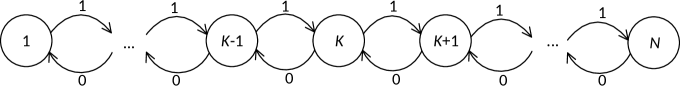
Figure 1: FSM of DC-free constraints

CS encoders can be described by finite state machines (FSMs) consisting of states, edges and labels. For example, the FSM of a DC-free constraint with $N$ different RDS values is shown in Fig. 1. The capacity of a constrained sequence $C$ is defined as [5]

$$C=\lim_{m\rightarrow\infty}\frac{\log_{2}{\cal N}(m)}{m}$$ (1)

where ${\cal N}(m)$ denotes the number of constraint-satisfying sequences of length $m$. Based on the FSM description and the adjacency matrix $\bf{D}$ [1], we can evaluate the capacity of a constraint by calculating the logarithm of $\lambda_{max}$ which is the largest real root of the determinant equation [5]

$$\det[{\bf{D}}-z{\bf{I}}]={\bf{0}}$$ (2)

where $\bf{I}$ is an identity matrix. The capacity is given as [5]

$$C=\log_{2}\lambda_{max}$$ (3)

with units bits of information per symbol.

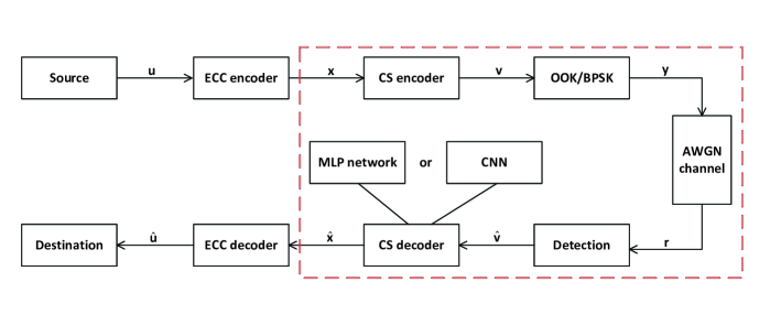
Figure 2: System model

II-B System model

We consider a typical wireless communication system as shown in Fig. 2. In particular, we consider visible light communications when demonstrating the use of DC-free codes, and wireless energy harvesting when demonstrating the use of RLL codes. Source bits $\bf{u}$ are encoded by an ECC encoder and a CS encoder to generate coded bits $\bf{x}$ and $\bf{v}$, respectively. The coded bits are then modulated to $\bf{y}$ and transmitted via an additive white Gaussian noise (AWGN) channel. We use on-off keying (OOK) modulation for VLC, and binary phase shift keying (BPSK) for wireless energy harvesting. The received bits are

$${\bf{r}}={\bf{y}}+{\bf{n}}$$ (4)

where ${\bf{n}}$ is the noise vector where each element is a Gaussian random variable with a zero mean and variance $\sigma^{2}$. The detector outputs symbol estimates $\bf{\hat{v}}$, and this sequence of estimates is decoded with the CS decoder and ECC decoder successively to generate the estimate $\bf{\hat{u}}$. In this paper we consider the framed components, and focus on the CS decoder that outputs $\bf{\hat{x}}$ as close as possible to $\bf{x}$. Throughout the paper we denote $|\bf{x}|$ as the size of vector $\bf{x}$.

II-C MLP networks and CNNs

The fundamentals of deep learning are comprehensively described in [36]. We employ both MLP networks and CNNs for CS decoding to predict $\bf{\hat{x}}$ given the input $\bf{\hat{v}}$. An MLP network has $L$ feed-forward layers. For each of the neurons in the MLP network, the output $\nu$ is determined by the input vector $\bf{t}$, the weights vector ${\bm{\theta}}$ and the activation function $g()$:

$${\nu=g({\bm{\theta}}\bf{t})}$$ (5)

where for the activation function we use the sigmoid function $g(z)=\frac{1}{1+\exp(-z)}$ and the rectified linear unit (ReLU) function $g(z)=\max\{0,z\}$. A deep MLP network consists of many layers; the $i$th layer performs the mapping ${\bf{f}}^{(i)}:\mathbb{R}^{t_{i}}\rightarrow\mathbb{R}^{m_{i}}$, where $t_{i}$ and $m_{i}$ are the lengths of the input vector and the output vector of that layer, respectively. The MLP network is represented by:

$${\bf{\hat{x}}}={\bf{f}}^{(L)}({\bf{f}}^{(L-1)}(...{\bf{f}}^{(2)}({\bf{f}}^{(1)}(\bf{\hat{v}}))))$$ (6)

The use of CNNs has recently achieved impressive performance in applications such as visual recognition, classification and segmentation, among others [36]. It employs convolutional layers to explore local features instead of extracting global features with fully connected layers as in MLP networks, thus greatly reducing the number of weights that need to be trained and making it possible for the network to grow deeper [37]. Different from visual tasks where the input colored images are represented by three dimensional vectors, the input vector $\bf{\hat{v}}$ in our task of CS decoding is a one dimensional vector. For a convolutional layer with $F$ kernels given as: ${\bf{q}}^{f}\in\mathbb{R}^{1\times|{\bf{q}}|},{f=1,...,F}$, the generated feature map ${\bf{\hat{p}}}^{f}\in\mathbb{R}^{1\times|{\bf{\hat{p}}}|}$ from the input vector ${\bf{\hat{v}}}\in\mathbb{R}^{1\times|{\bf{\hat{v}}}|}$ satisfies the following dot product:

$${p}^{f}_{i}=\sum_{l=0}^{|{\bf{q}}|-1}q^{f}_{l}{\hat{v}}_{1+s(i-1)+l}$$ (7)

where $s\geq 1$ is the stride. CNNs benefit from weight sharing that exploits the spatial correlations of images and thus usually require fewer weights to be trained. Usually convolutional layers are followed by pooling layers such that high-level features can be extracted at the top layers. However, as we will show, pooling may not fit well in CS decoding and therefore our implementation of CNN does not include pooling layers.

III Deep learning-based decoding for fixed-length CS codes

III-A The fixed-length 4B6B code in visible light communications

VLC refers to short-range optical wireless communication using the visible light spectrum from 380 nm to 780 nm, and has gained much attention recently [3]. The simplest VLC relies on OOK modulation, which is realized with DC-free codes to generate a constant dimming level of $50\%$. Three types of FL DC-free codes have been used in VLC standards to adjust dimming control and reduce flicker perception: the Manchester code, the 4B6B code and the 8B10B code [3]. We use the 4B6B code as a running example in this section to discuss FL CS codes.

The 4B6B code satisfies the DC-free constraint with $N=5$, which has a capacity of 0.7925 [1]. The codebook has 16 source words as shown in Table I [3]. Each source word has a length of 4 and is mapped to a codeword of length 6, which results in a code rate $R$ of $2/3$, and therefore an efficiency $\eta=R/C$ of $84.12\%$. In the remainder of this section we discuss how we use DNNs to decode the 4B6B code. We employ both MLPs and CNNs, and compare their performance.

TABLE I: Codebook of the 4B6B DC-free VLC code: $R=2/3,\eta=84.12\%$

Source word	Codeword	Source word	Codeword
0000	001110	1000	011001
0001	001101	1001	011010
0010	010011	1010	011100
0011	010110	1011	110001
0100	010101	1100	110010
0101	100011	1101	101001
0110	100110	1110	101010
0111	100101	1111	101100

III-B Training method

In order to constrain the size of the training set, we follow the training method in [28] where the DNN was extended with additional layers of modulation, noise addition and detection that have no additional parameters that need to be trained. Therefore, it is sufficient to work only with the sets of all possible noiseless codewords ${\bf{v}}\in\mathbb{F}_{2}^{|\bf{v}|},\mathbb{F}_{2}\in\{0,1\}$, i.e., training epoches, as input to the DNNs. For the additional layer of detection, we calculate the log-likelihood ratio (LLR) of each received bit and forward it to the DNN. We use the mean squared error (MSE) as the loss function, which is defined as:

$$L_{MSE}=\frac{1}{|{\bf{x}}|}\sum_{i}(x_{i}-\hat{x}_{i})^{2}.$$ (8)

Both the MLP networks and CNNs employ three hidden layers, details of which are discussed in the next section. We aim at training a network that is able to generalize, that is we train at a particular signal-to-noise ratio (SNR) and test it within a wide range of SNRs. The criterion for model selection that we employ follows [28], which is the normalized validation error (NVE) defined as:

$$NVE(\rho_{t})=\frac{1}{S}\sum_{s=1}^{S}\frac{BER_{DNN}(\rho_{t},\rho_{v,s})}{BER_{MAP}(\rho_{v,s})},$$ (9)

where $\rho_{v,s}$ denotes the $S$ different test SNRs. $BER_{DNN}(\rho_{t},\rho_{v,s})$ denotes the BER achieved by the DNN trained at SNR $\rho_{t}$ and tested at SNR $\rho_{v,s}$, and $BER_{MAP}(\rho_{v,s})$ denotes the BER of MAP decoding of CS codes at SNR $\rho_{v,s}$. The networks are trained with a fixed number of epoches that we will present in the next section.

III-C Results and outlook

We use the notation ${\bf{h}}=[h_{1},h_{2},...,h_{L}]$ to represent a network with $L$ hidden layers, where $h_{l}$ denotes the number of neurons in the fully connected layer $l$, or the number of kernels in the convolutional layer $l$. In recent works that apply DNNs to decode ECCs, the training set explodes rapidly as the source word length grows. For example, with a rate 0.5 $(n=1024,k=512)$ ECC, one epoch consists of $2^{512}$ possibilities of codewords of length 1024, which results in very large complexity and makes it difficult to train and implement DNN-based decoding in practical systems [28, 29, 31, 32]. However, we note that in FL CS decoding, this problem does not exist since CS source words are typically considerably shorter, possibly only up to a few dozen symbols [1, 6, 7, 8, 9, 16, 10, 11, 12, 13, 17, 14, 15]. This property fits deep learning based-decoding well.

III-C1 BER performance

Frame-by-frame decoding

First we consider frame-by-frame transmission, where the 4B6B codewords are transmitted and decoded one-by-one, i.e., $|{\bf{v}}|=6$. We will later consider processing multiple frames simultaneously to improve the system throughput. Note that in the VLC standard, two 4B6B look-up tables can be used simultaneously [3].

We compare performance of deep learning-based decoding with conventional LUT decoding that generates hard-decision bits. That is, the traditional detector estimates the hard decision $\hat{\bf{v}}$, and the CS decoder attempts to map $\hat{\bf{v}}$ to a valid source word to generate $\hat{\bf{x}}$. If the decoder is not able to locate $\hat{\bf{v}}$ in the code table due to erroneous estimation at the detector, the decoder determines the codeword that is closest to $\hat{\bf{v}}$ in terms of Hamming distance, and then outputs the corresponding source word. We also implement the maximum likelihood (ML) decoding of CS codes, where the codeword with the closest Euclidean distance to the received noisy version of the codeword is selected and the corresponding source word is decoded. We assume equiprobable zeros and ones in source sequences, thus ML decoding is equivalent to MAP decoding of CS codes since each codeword has an equal occurrence probability.

TABLE II: Parameters of the MLP networks and CNNs trained for CS decoding with different frames

	MLP		CNN
# of frame	# of neurons	# of parameters	# of kernels	# of parameters	epoches
1	[32,16,8]	924	[8,12,8]	760	4$\mathrm{e}$+4
2	[64,32,16]	3576	[8,14,8]	1374	3$\mathrm{e}$+4
3	[128,64,32]	13164	[8,16,8]	2372	3$\mathrm{e}$+4
4	[128,128,64]	29008	[16,16,12]	5676	2.5$\mathrm{e}$+3
5	[256,128,64]	50338	[16,32,12]	9536	2.5$\mathrm{e}$+3

Table II shows the parameters of the MLP networks and the CNNs for a variety of tasks, and the number of epoches used for each network. The DNNs are initialized using Xavier initialization [38], and trained at an SNR of 1 dB using Adam for stochastic gradient descent optimization [39]. With $|{\bf{v}}|=6$, the parameters of the proposed networks are shown in row three of Table II. The MLP network we trained for frame-by-frame decoding has three hidden layers [32,16,8] and 924 trainable parameters. Its BER performance is shown in Fig. 3, which shows that DNN-based decoding achieves a BER that is very close to MAP decoding of CS codes, and outperforms the conventional LUT decoding described above by $\sim$2.2 dB.

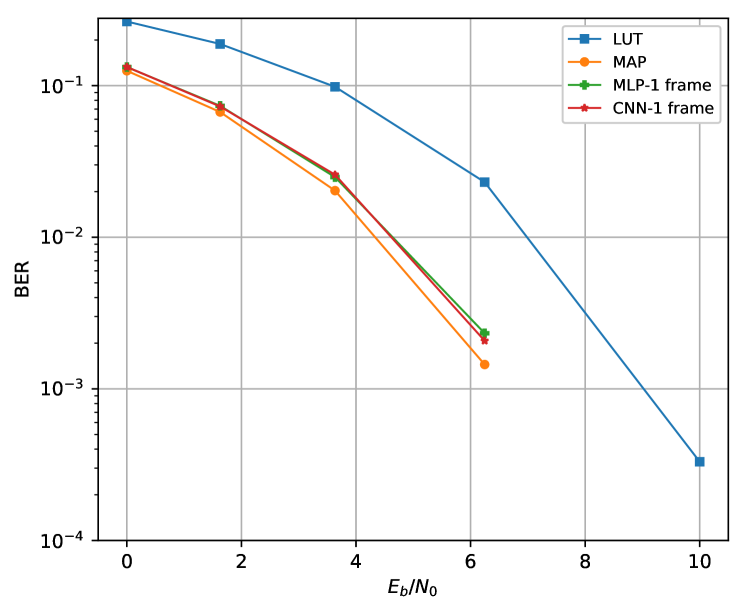
Figure 3: Comparison of BER performance with frame-by-frame transmission, i.e., $|{\bf{v}}|=6$

We then investigate employing CNNs for this task. With ECC decoding, CNNs and MLP networks have similar number of weights in order to achieve similar performance [31]. In the following we outline our findings that are unique to CS decoding.

TABLE III: Structures of the CNNs for CS decoding

layer	kernal size / stride	input size	padding
OOK	N/A	$1\times|{\bf{v}}|$	N/A
Adding noise	N/A	$1\times|{\bf{v}}|$	N/A
LLR	N/A	$1\times|{\bf{v}}|$	N/A
Convolution	$1\times 3$ / 1	$1\times|{\bf{v}}|$	no
Convolution	$1\times 3$ / 1	$1\times(|{\bf{v}}|-2)\times h_{1}$	yes
Convolution	$1\times 3$ / 1	$1\times(|{\bf{v}}|-2)\times h_{2}$	yes
Fully connected	N/A	$1\times((|{\bf{v}}|-2)\times h_{3})$	N/A
Sigmoid	N/A	$1\times(|{\bf{x}}|)$	N/A

In Table III we outline the structure of the CNNs we apply for CS decoding. ReLU is used as the activation function for each convolutional layer. We note that CS codes always have inherent constraints on their codewords such that they match the characteristics of the channel. For example, the 4B6B code in Table I always has an equal number of logic ones and logic zeros in each codeword, and the runlength is limited to four in the coded sequence for flicker reduction. These low-level features can be extracted to enable CNNs to efficiently learn the weights of the kernels, which results in a smaller number of weights that need to be trained in the training phase compared to MLP networks. For example, although similar BER performance is achieved by the [32, 16, 8] MLP network and the [6, 10, 6] CNN, the number of weights in the CNN is only $82\%$ of that in the MLP network. With larger networks the reduction in the number of weights that need to be trained is more significant, as we show in the next subsection.

Another finding we observe during training of a CNN is that pooling layers, which are essential component structures in CNNs for visual tasks, may not be required in our task. The reason is that in visual tasks, pooling is often used to extract high-level features of images such as shapes, edges or corners. However, CS codes often possess low-level features only, and we find that adding pooling layers may not assist CS decoding. Therefore, no pooling layer is used in our CNNs, as indicated in Table III. Fig. 3 shows that use of a CNN achieves similar performance to the use of an MLP network, and that it also approaches the performance of MAP decoding.

TABLE IV: Test phase time and space complexity of the MLP networks and CNNs used in Table II

	MLP		CNN
# of frame	Time (FLOPs)	Space (MBytes)	Time (FLOPs)	Space (MBytes)
1	8.64$\mathrm{e}$+2	0.0035	2.53$\mathrm{e}$+3	0.0032
2	3.46$\mathrm{e}$+3	0.014	7.6$\mathrm{e}$+3	0.0063
3	1.29$\mathrm{e}$+4	0.05	1.42$\mathrm{e}$+4	0.011
4	2.87$\mathrm{e}$+4	0.11	3.48$\mathrm{e}$+4	0.025
5	4.99$\mathrm{e}$+4	0.19	8.33$\mathrm{e}$+4	0.043

Improving the throughput

We now consider processing multiple frames in one time slot in order to improve the system throughput. The system throughput can be enhanced by increasing the optical clock rate, which has its own physical limitations, or by processing multiple 4B6B codewords in parallel. The VLC standard allows two 4B6B codes to be processed simultaneously [3]. Now we show that DNNs can handle larger input size where $|{\bf{v}}|$ is a multiple of 6, thus system throughput can be enhanced by using one of those DNNs or even using multiple DNNs in parallel.

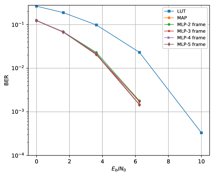
Figure 4: BER performance of MLP networks with multiple frames processed simultaneously, $|{\bf{v}}|=12,18,24,30$

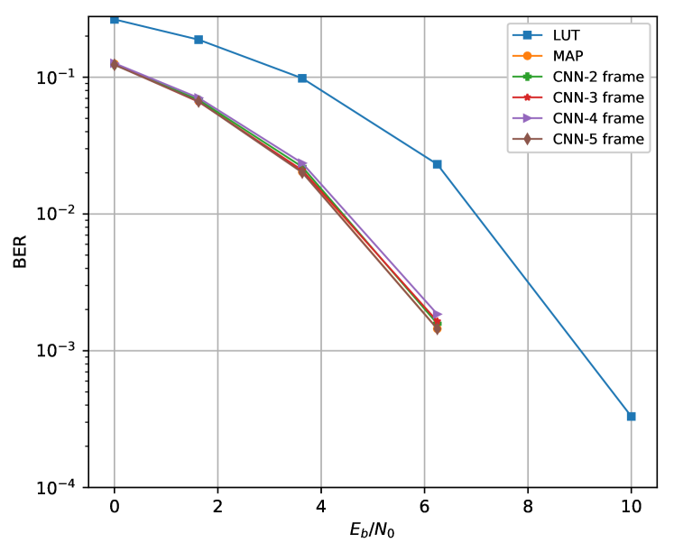
Figure 5: BER performance of CNNs with multiple frames processed simultaneously, $|{\bf{v}}|=12,18,24,30$

Figs. 4 and 5 present the BER performance of MLP networks and CNNs respectively. The parameters of those networks are shown in Table II, where rows 3, 4, 5 and 6 correspond to the parameters of the proposed networks with $|{\bf{v}}|=12,18,24,30$, respectively. These figures demonstrate that both MLP networks and CNNs are able to achieve BERs very close to MAP decoding, while the CNNs have a smaller number of weights that need to be trained at the training phase compared to the MLP networks for the reasons outlined above. With larger $|{\bf{v}}|$, CNN becomes more advantageous in extracting the low-level features from the longer input sequences and learning the weights, and thus the reduction in the number of trainable parameters with a CNN is more significant. For example, when processing five frames simultaneously, the CNN has less than $1/5$ of the parameters that need to be trained for the MLP network. Note that we consider the number of parameters in the networks shown in Table II to be small, e.g., ResNet [37] has a few million parameters to train.

Following the study in [40, 41], we now consider the time and space complexities of the proposed networks at the test phase. We study the theoretical time complexity instead of actual running time, because the actual running time can be sensitive to specific hardware and implementations. The time complexity of an MLP network is measured, with units of floating-point operations (FLOPs), as:

$$O\bigg{(}\sum_{l=1}^{L+1}h_{l-1}\cdot h_{l}\bigg{)},$$ (10)

where $h_{0}=|\bf{v}|$ and $h_{L+1}=|\bf{x}|$.

The space complexity of the MLP networks is measured, with units of bytes, as:

$$O\bigg{(}4\sum_{l=1}^{L+1}\Big{(}h_{l-1}\cdot h_{l}+(1\cdot m_{l})\Big{)}+4|\bf{v}|\bigg{)},$$ (11)

where $m_{l}$ is the length of the output of layer $l$ and $m_{L+1}=|\bf{x}|$. $h_{l-1}\cdot h_{l}$ is the memory needed to store the weights of the network, $1\cdot m_{l}$ is the memory needed to store the output of each layer, and $|\bf{v}|$ is the memory needed to store the input vector.

For CNNs, the time complexity of a CNN is measured, with units of floating-point operations (FLOPs), as:

$$O\bigg{(}\sum_{l=1}^{L+1}h_{l-1}\cdot(1\cdot{\cal K}_{l})\cdot h_{l}\cdot(1\cdot m_{l})\bigg{)},$$ (12)

where $h_{0}=1$ and $h_{L+1}=|\bf{x}|$, and ${\cal K}_{l}$ denotes the length of the kernel at layer $l$. $m_{l}$ is the length of the output of layer $l$. ${\cal K}_{L+1}=m_{L}$, $m_{L+1}=1$ [42].

The space complexity of the CNNs is measured, with units of bytes, as:

$$O\bigg{(}4\sum_{l=1}^{L+1}\Big{(}(1\cdot{\cal K}_{l})\cdot h_{l-1}\cdot h_{l}+(1\cdot m_{l})\cdot h_{l}\Big{)}+4|\bf{v}|\bigg{)}.$$ (13)

In Table IV, we provide the time and space complexity of the networks we described in Table II. It is seen that, at the test phase, CNNs have higher time complexity since convolutional layers are time-consuming at the test phase [40]. However, CNNs have less space complexity due to weight sharing, and they require less memory. Nevertheless, we note that all networks listed in Table II are small and have relatively low implementation complexity when compared to other modern DNNs, for example, VGG-16 [43] which has time complexity of 1.55$\mathrm{e}$+10 FLOPs and space complexity of 5.53$\mathrm{e}$+2 MB [40]. Therefore, we anticipate that it will be practical to achieve further improvement of system throughput with larger and deeper networks.

III-C2 Paving the way to FL capacity-achieving CS codes

As we outlined in Section I, it is not an easy task to implement capacity-achieving FL CS codes. As determined by equations (1)-(3), the capacity of a constraint is irrational in all but a very limited number of cases [44], and can be typically approached with fixed-length codes of rate $R=k/n$ only with very large $k$ and $n$ values. This hinders implementation of LUT encoding and decoding for capacity-achieving CS codes. For example, as shown in Section II-B, the 4B6B code achieves $84.12\%$ of the capacity of a DC-free code with 5 different RDS values, which has $C=0.7925$. In Table V we list, for increasing values of $k$, values of $n$ that result in high code rates. This table shows that with $k=11,15,19$, it could be possible to construct fixed-length codes with efficiencies that exceed $99\%$. With $k$ as large as $79$ and $n=100$, the code would have rate 0.79 and efficiency $99.68\%$. However, an LUT codebook with $2^{k}$ source word-to-codeword mappings becomes impractical to implement as $k$ grows large. Other examples are the $k$-constrained codes recently developed for DNA-based storage systems in [4]. Those fixed-length 4-ary $k$-constrained codes have rates very close to the capacity, however they require very large codebooks. For example, with method B in [4], for the $k$-constrained code with $k=1,2,3,4$, the codebooks have $4^{10},4^{38},4^{147},4^{580}$ source word-to-codeword mappings respectively.

TABLE V: Highest code rate and efficiency with fixed-length CS codes for the DC-free constraint with five different RDS values, $C=0.7925$

$k$	$n$	$R$	$\eta$	$k$	$n$	$R$	$\eta$
1	2	0.5000	63.09%	11	14	0.7857	99.14%
2	3	0.6667	84.12%	12	16	0.7500	94.64%
3	4	0.7500	94.64%	13	17	0.7647	96.49%
4	6	0.6667	84.12%	14	18	0.7778	98.14%
5	7	0.7143	90.13%	15	19	0.7895	99.62%
6	8	0.7500	94.64%	16	21	0.7619	96.14%
7	9	0.7778	98.14%	17	22	0.7727	97.51%
8	11	0.7273	91.77%	18	23	0.7826	98.75%
9	12	0.7500	94.64%	19	24	0.7917	99.89%
10	13	0.7692	97.06%	20	26	0.7692	97.06%

With DNNs, however, it becomes practical to handle a large set of source word-to-codeword mappings which used to be considered impractical with LUT decoding. This paves the way for practical design and implementation of fixed-length capacity-achieving CS codes. Appropriate design of such codes is a practice of using standard algorithms from the rich theory of CS coding, such as Franaszek’s recursive elimination algorithm [6], or the sliding-block algorithm [45, 46] with large $k$ and $n$ values to determine the codebooks. We propose implementing both the encoder and the decoder with DNNs. Although here we focus on decoding, similar to DNN-based decoders, CS encoders map noiseless source words to codewords, and can also be implemented with DNNs.

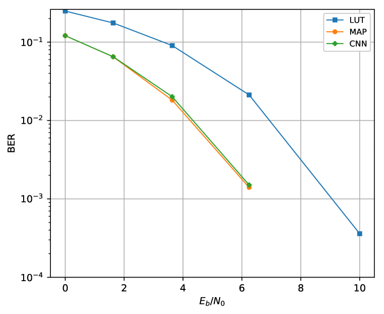
Figure 6: BER performance of DNN-based decoding for a constrained sequence code with $2^{20}$ possibilities of mappings

We now demonstrate that the proposed DNN-based  decoders are able to map long received words from a CS code to their corresponding source words. We concatenate five 4B6B codebooks, where each 4B6B codebook is randomly shuffled in terms of its source word-to-codeword mappings, to generate a large codebook with $2^{20}$ entries of mappings. We train and test a CNN with ${\bf{h}}=[16,32,12]$ that has 9536 weights to perform decoding. From Fig. 6, we can see that this CNN is capable of decoding the received noisy version of the large set of received words. The BER is close to MAP decoding, and outperforms the LUT decoding approach that we implemented as a benchmark. Therefore, the design and implementation of DNN-based CS decoding is practical with long CS codewords because of their low-level features that we can use to our advantage to simplify decoding.

We also note that DNNs that are proposed in communication systems could have many more parameters than the 9536 we use in this network. For example, [47] proposes an MLP network with 4 hidden layers where each layer has 512 neurons, which results in at least $512\times 512\times 3=786432$ parameters. Thus a larger CNN can be trained to decode fixed-length capacity-approaching CS codes with longer codewords. Having found that CNNs require many fewer parameters to train compared to MLP networks, we continue using CNNs for decoding variable-length CS codes in the next section.

IV Deep learning-based decoding for VL CS codes

IV-A VL CS codes

It has been recently reported in the literature that VL CS codes can exhibit higher code rates and simpler codebooks than their FL counterparts. Capacity-approaching VL codes have been designed with a single state [19, 20, 21, 22] and multiple states [23] in their codebooks. With a one-to-one correspondence between the lengths of VL source words and VL codewords, and the assumption of independent and equiprobable zeros and ones in the source sequence, the average code rate $\overline{R}$ is [19, 20]

$$\overline{R}=\frac{{\bar{k}}}{{\bar{n}}}=\frac{{\sum\limits_{{s_{i}}}{{2^{-{s_{i}}}}}{s_{i}}}}{{\sum\limits_{{o_{i}}}{{2^{-{s_{i}}}}}{o_{i}}}}$$ (14)

where $s_{i}$ is the length of the $i$-th source word that is mapped to the $i$-th codeword of length $o_{i}$. The efficiency of a code is defined as $\eta=\overline{R}/C$.

IV-A1 Codes for wireless energy harvesting

Wireless energy harvesting requires avoidance of battery overflows or underflows at the receiver, where overflow represents the event that energy is received but the battery is full, while underflow occurs when energy is required by the receiver when the battery is empty [2]. Consider an energy harvesting system where logic one coded bits carry energy, bit logic zeros do not. In such cases, $(d,k)$ RLL codes have been proposed to work in regimes where overflow protection is the most critical. By substituting all logic zeros with logic ones and vice versa, use of these RLL codes have been proposed for regimes where underflow protection is the most critical [2, 48].

Following the capacity-approaching VL code construction technique in [19, 20], we construct a single-state codebook for the VL $(d=1,k=3)$ RLL code given in Table VI that achieves $98.9\%$ of capacity, and we use this code as a running example throughout this section. As a comparison, note that a widely used $(d=1,k=3)$ FL RLL code is the MFM code with $\eta=91\%$ [1], which demonstrates the increase in efficiency that is possible with use of VL CS codes.

TABLE VI: Codebook of a $(d=1,k=3)$ RLL code with efficiency of $98.9\%$

Source word	Codeword
$0$	01
$10$	001
$11$	0001

IV-A2 Codes for visible light communications

Table VII (from [23]) presents a VL DC-free codebook that has two encoding states $\sigma_{1},\sigma_{2}$ and satisfies exactly the same constraint as the 4B6B code in Table I. $\alpha(\sigma_{i})$ and $\beta(\sigma_{i})$ denote the output codewords and the next states. This code has an average code rate $\overline{R}=0.7857$ and an average efficiency $\eta=99.14\%$, which is significantly higher than the 4B6B code. It also has fewer codewords compared to the 4B6B code.

TABLE VII: Codebook of DC-free code with $\eta=99.14\%$ and an RDS value of 5

Source word	$\alpha(\sigma_{1})$	$\beta(\sigma_{1})$	$\alpha(\sigma_{2})$	$\beta(\sigma_{2})$
$00$	$11$	$\sigma_{2}$	00	$\sigma_{1}$
$010$	$0111$	$\sigma_{2}$	1000	$\sigma_{1}$
$011$	$0101$	$\sigma_{1}$	0101	$\sigma_{2}$
$100$	$0110$	$\sigma_{1}$	0110	$\sigma_{2}$
$101$	$1011$	$\sigma_{2}$	0100	$\sigma_{1}$
$110$	$1001$	$\sigma_{1}$	1001	$\sigma_{2}$
$111$	$1010$	$\sigma_{1}$	1010	$\sigma_{2}$

In the following we demonstrate how we employ CNNs for VL CS decoders to improve the system throughput and reduce error rates.

IV-B Conventional bit-by-bit processing

Since the VL CS codes in Tables VI and VII are instantaneous codes, when no errors occur during transmission, the received sequences can be accurately segmented at the decoder and decoded with bit-by-bit processing. Details of this process are given in Algorithm 1, where ${\bf{\widehat{v}}}_{i}^{j}$ denotes the sub-vector of ${\bf{\widehat{v}}}$ starting from the $i$th position and ending at the $j$th position. Whenever the receiver receives another bit, it attempts to match the current processed sequence with a codeword in the codebook. If the receiver is unable to find a match, it then takes the next received bit and repeats the process. For example, with the single-state $(d=1,k=3)$ RLL codebook in Table VI, the RLL coded sequence ${\bf{\widehat{v}}}=010001001$ is correctly decoded into $01110$ by the decoder that uses Algorithm 1.

Algorithm 1 Conventional bit-by-bit decoding of error-free VL CS coded sequences

0:  

1:  $\bf{\hat{v}}$, the codebook

2:  $cur\_pos\_head\leftarrow 1,cur\_pos\leftarrow 1$

2:  

3:  while $cur\_pos\_head\leq|\bf{\hat{v}}|$ do

4:     if ${\bf{\hat{v}}}_{cur\_pos\_head}^{cur\_pos}$ is a valid codeword then

5:        decode ${\bf{\hat{v}}}_{cur\_pos\_head}^{cur\_pos}$ into the corresponding source word

6:        $cur\_pos\leftarrow cur\_pos+1$;

7:        $cur\_pos\_head\leftarrow cur\_pos$;

8:     else

9:        $cur\_pos\leftarrow cur\_pos+1$;

10:     end if

11:  end while

If errors occur during transmission, the decoder will have low probability of segmenting the received sequence correctly, and hence may lose synchronization. For example, assume the encoded $(d=1,k=3)$ RLL sequence is ${\bf{v}}=010001001$, but that noise causes the fifth bit to be detected in error such that the erroneously detected sequence is ${\bf{\widehat{v}}}=010011001$. After correctly decoding codeword $01$ into 0, the bit-by-bit decoder would determine that the next codeword is 001 and hence would perform incorrect codeword segmentation and therefore would output an incorrect decoded sequence. Note that due to incorrect segmentation, synchronization is lost in the sense that codeword boundaries are incorrectly determined. This loss of synchronization, i.e., incorrect identification of the start and end positions of each codeword, may result in error propagation. One possible algorithm for decoding VL CS sequences in case of transmission errors is described in Algorithm 2 in the Appendix, which helps recover synchronization, but is unable to correct detection errors.

Therefore, there are two drawbacks of conventional decoding for VL CS codes: i) since decoding is processed bit-by-bit, the system throughput is limited especially when errors occur during transmission which requires more processing to be done, and ii) since bit-by-bit decoding is in fact greedy and takes into account only the local information by considering only the next few bits when trying to find a codeword match, it is very likely that the decoder generates erroneous output and/or loses synchronization. To tackle these drawbacks, we propose using CNNs to help the decoder perform batch-processing to increase the system throughput and reduce the error rate such that the CNN-aided decoder can still generate correct output sequences in the event of transmission errors.

IV-C CNN-aided decoding of VL CS codes

We propose using CNNs for codeword segmentation of the received sequences to enable batch-processing. Consider the $(d=1,k=3)$ RLL code in Table VI. As illustrated in Fig. 7(a), $\bf{\widehat{v}}$ is passed into the decoder, where the CNN performs segmentation and generates a codeword boundary vector $\bf{\gamma}$ in one shot. Once $\bf{\gamma}$ is obtained, the decoder enters the post-processing phase and generates the source sequence by looking directly at the codeword boundaries and finding the corresponding source words in Table VI. In this way the system throughput can be improved. Moreover, as illustrated in Fig. 7(b), when determining the next codeword boundary, since the CNN considers an entire batch at a time, it also makes use of bits that are not close to the current codeword. In other words, the CNN not only makes use of local information, but also takes advantages of global information such that even if the received sequence is in error, the CNN may still be able to help the decoder stay synchronized and correctly recover the source sequence. Note that to take advantage of the full received information, in our implementation the input vector of the CNN is the noisy received sequence $\bf{r}$ instead of the demodulated bit sequence $\bf{\widehat{v}}$.

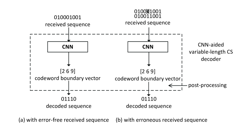
Figure 7: Illustration of the CNN-aided VL CS decoder

We propose that the codeword segmentation problem is analogous to two-dimensional object detection in computer vision. In object detection, the output is the coordinates $(a_{1},b_{1})$, $(a_{1},b_{2})$, $(a_{2},b_{1})$, $(a_{2},b_{2})$ of the four corners of the boxed rectangle that captures the detected object. Our CNN works with the one-dimensional input sequence $\bf{r}$, hence for the $i$th detected codeword in $\bf{r}$ it suffices to output two scalars $\gamma_{i}=(\gamma_{i,start},\gamma_{i,end})$ that correspond to the start and end positions of that codeword, where $\gamma_{i,end}=\gamma_{i+1,start}-1$. Therefore, the output vector of the CNN is ${\bm{\gamma}}=[\gamma_{1},\gamma_{2},...,\gamma_{|{\bf{\gamma}}|}]$ which indicates the start and end positions of all codewords segmented from $\bf{r}$, which are exactly the synchronization positions. Furthermore, we propose to set the input size $|\bf{r}|$ of the CNN to be the largest packet size $L_{max}$ of the transmission system, such that the CNN is able to perform codeword segmentation with the largest packet and hence the start position of the first detected codeword is $\gamma_{1,start}=0$. Therefore, ${\bm{\gamma}}$ is simplified to ${\bm{\gamma}}=[\gamma_{1,end},\gamma_{2,end},...,\gamma_{|{\bf{\gamma}}|,end}]$ where each element indicates a codeword boundary, which is a synchronization position. When the received packet has size smaller than $L_{max}$, the packet is augmented with padding symbols to match the input size of the CNN. Details of the padding are discussed below.

Training method

The data generation phase is the same as in Section III.B where the CNN is extended with additional layers that have no parameters such that it suffices to work only with the set of all possible noiseless codewords, except that we do not use the LLR layer in our CNN-aided VL CS decoder. From the codebook in Table VI, it is readily seen that the longest source sequence that can generate a coded sequence of length $L_{max}$ is $L_{max}/2$. We generate all possible source sequences of length $L_{max}/2$ and encode them into coded sequences that are at most of length $L_{max}$. If a received sequence has length smaller than $L_{max}$, it is padded with invalid symbol values (which we denote here as –1) such that the resulting length is $L_{max}$. The output vector $\bm{\gamma}$ has length $|\bm{\gamma}|=L_{max}/2$, where each of the elements is a codeword boundary, i.e., a synchronization position. If the number of codewords in the coded sequence is smaller than $L_{max}/2$, the rest of the elements are padded with symbols $L_{max}+1$ that indicate the last valid codeword boundary has been passed. At the post-processing phase, if the decoder encounters a value of $L_{max}+1$, it interprets this to indicate that the segmentation of the entire batch is completed, and it will finish decoding the current batch.

To illustrate, consider the situation in Fig. 7(a). If we set $L_{max}=10$, then the received sequence is padded with invalid symbol values, resulting in a vector of $[0,1,0,0,0,1,0,0,1,-1]$ that has length 10, and the output codeword boundary vector is ${\bm{\gamma}}=[2,6,9,11,11]$.

The criterion for model selection is similar to (9), except that we employ the block error rates (BLERs) instead of the bit error rates. The NVE in this case is defined as:

$$NVE(\rho_{t})=\frac{1}{S}\sum_{s=1}^{S}\frac{BLER_{CNN}(\rho_{t},\rho_{v,s})}{BLER_{raw}(\rho_{v,s})},$$ (15)

where $\rho_{v,s}$ denotes the $S$ different test SNRs. $BLER_{CNN}(\rho_{t},\rho_{v,s})$ denotes the BLER of the decoded source sequence achieved by the CNN-aided decoder trained at SNR $\rho_{t}$ and tested at SNR $\rho_{v,s}$, and $BLER_{raw}(\rho_{v,s})$ denotes the raw BLER, i.e., the BLER of the received sequence $\bf{\widehat{v}}$, at SNR $\rho_{v,s}$. We use the MSE in (8) as the loss function.

TABLE VIII: Structures of the CNNs for VL CS decoding

layer	kernal size / stride	input size	padding
BPSK/OOK	N/A	$1\times|{\bf{r}}|$	N/A
Adding noise	N/A	$1\times|{\bf{r}}|$	N/A
Convolution	$1\times 4$ / 1	$1\times|{\bf{r}}|$	no
Convolution	$1\times 5$ / 1	$1\times(|{\bf{r}}|-3)\times h_{1}$	no
Convolution	$1\times 5$ / 1	$1\times(|{\bf{r}}|-7)\times h_{2}$	no
Fully connected	N/A	$1\times((|{\bf{r}}|-11)\times h_{3})$	N/A
Fully connected	N/A	$1\times 80$	N/A
Fully connected + ReLU	N/A	$1\times 30$	N/A

Results and outlook

In our experiments we set ${|\bf{r}|}=L_{max}=12$. The structure of the CNN we developed is shown in Table VIII, where ${\bf{h}}=[16,32,20,80,30]$. The first three layers are convolutional layers and the last two layers are fully connected layers, resulting in 10188 trainable parameters. ReLU is used as the activation function for each convolutional layer, and for the final output. The number of epoches used for training this network is 1$\mathrm{e}$+5. We observed during experimentation that, different from the prior-art (and Section III in this paper) that employs deep learning for channel decoding where the DNNs are trained at relatively small values of SNR, in the codeword segmentation problem we find that the CNN should be trained at relatively large SNRs in order to work well. The intuitive reasoning for this observation is that codeword segmentation is inspired from object detection in computer vision, and in object detection the CNN should be trained with ground-truth samples. Similarly, in the codeword segmentation problem, the CNN would be trained with codewords plus relatively small noise, i.e., “ground-truth samples”, as input.

The result for the $(d=1,k=3)$ RLL code is shown in Fig. 8, where the CNN is trained at 10dB. It is clear that the CNN-aided decoder has smaller BLER than the raw BLER, indicating that the CNN is able to make use of global information to search for the global optimum instead of only the local optimum when performing codeword segmentation, and therefore has the capability of correctly detecting the codeword boundaries and maintaining synchronization even when the received sequence is in error. In low-to-medium SNR regions the CNN-aided decoder achieves $\sim$1 dB performance gain. Therefore, the CNN-aided decoder is not only able to improve the system throughput by enabling one-shot decoding, but it also has some error-correction capabilities.

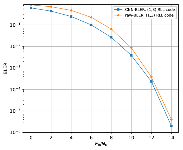
Figure 8: Comparison of BLER performance for the VL $(d=1,k=3)$ RLL code

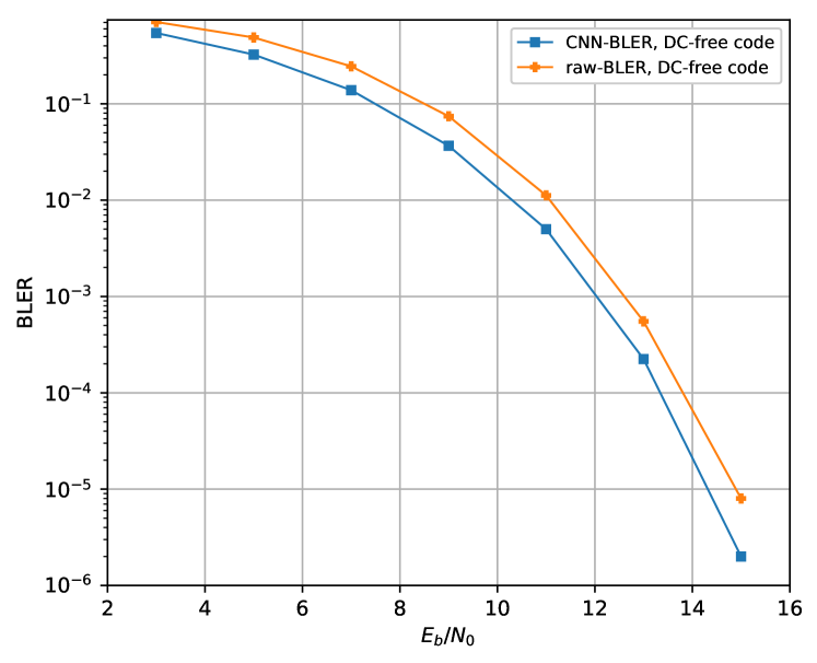
Figure 9: Comparison of BER performance for the VL DC-free code

We now show that our approach also works for multi-state codes where state transitions occur during encoding and hence the state information is implicitly carried in coded sequences. We employ the multi-state DC-free code in Table VII and train a CNN that has the same structure as in Table VIII to perform codeword segmentation. We note that, different from the $(d=1,k=3)$ RLL code in Table VI, although for this DC-free code the CNN is also able to perform codeword segmentation and help maintain synchronization, direct translation from $\bf{\gamma}$ to codewords is not possible since there is more than one codeword that has length 4. Therefore, during the post-processing phase the decoder performs soft-decision decoding based on the knowledge of $\bf{\gamma}$. In Fig. 9, we present the BLER of source sequences after the CNN-aided decoder, and compare it to the raw BLER. The CNN is trained at 11dB. Similar to the $(d=1,k=3)$ RLL code, apart from the ability of increasing the system throughput, the CNN demonstrates error-correction capabilities such that it may still correctly perform codeword segmentation when errors occur during transmission, and also provides $\sim$1 dB performance gain in low-to-medium SNR regions. Therefore, the CNN-aided decoder is able to learn the inherent state information in the multi-state coded sequences, improve the system throughput, help maintain synchronization by correctly performing codeword segmentation, and reduce the error rate. Lastly, we note that those CNN-aided decoders are practical for VL CS codes, and that a larger batch could be processed with a larger CNN in an actual implementation.

V conclusion

In this paper, we introduced deep learning-based decoding for FL and VL CS codes. For FL CS decoding, we studied two types of DNNs, namely MLP networks and CNNs, and found that both networks can achieve BER performance close to MAP decoding as well as improve the system throughput, where CNNs have smaller number of trainable parameters than MLP networks since they are able to efficiently exploit the inherent constraints imposed on the codewords. Furthermore, we showed that the design and implementation of FL capacity-achieving CS codes that have been considered impractical becomes practical with deep learning-based decoding, paving the way to deploying highly efficient CS codes in practical communication and data storage systems. We then developed CNNs for one-shot batch-processing of VL CS codes that exhibit higher code rates than their FL counterparts. We employed CNN-aided decoding for both single-state and multi-state VL CS codes, and showed that the CNN-aided decoder is not only able to improve the system throughput, but also has the capability of maintaining synchronization and performing error correction.

Appendix A An algorithm for bit-by-bit decoding of VL CS codes

Algorithm 2 Conventional bit-by-bit VL CS decoding when errors occur during transmission

0:  

1:  $\bf{\hat{v}}$, the codebook

2:  $l_{max}$: the maximum length of codewords in the codebook

3:  $cur\_pos\_head\leftarrow 1,cur\_pos\leftarrow 1$

3:  

4:  while $cur\_pos\_head\leq|\bf{\hat{v}}|$ do

5:     if $cur\_pos-cur\_pos\_head+1\leq l_{max}$ then

6:        if ${\bf{\hat{v}}}_{cur\_pos\_head}^{cur\_pos}$ is a valid codeword then

7:           decode ${\bf{\hat{v}}}_{cur\_pos\_head}^{cur\_pos}$ into the corresponding source word

8:           $cur\_pos\leftarrow cur\_pos+1$;

9:           $cur\_pos\_head\leftarrow cur\_pos$;

10:        else

11:           $cur\_pos\leftarrow cur\_pos+1$;

12:        end if

13:     else

14:        $/*$ no match is found in the codebook $*/$

15:        $cur\_pos\leftarrow cur\_pos\_head+1$;

16:        while $cur\_pos\leq|\bf{\hat{v}}|$ do

17:           for $tmp\_start\_pos$ in $[cur\_pos\_head,cur\_pos]$ do

18:              if ${\bf{\hat{v}}}_{tmp\_start\_pos}^{cur\_pos}$ is a valid codeword then

19:                 decode ${\bf{\hat{v}}}_{tmp\_start\_pos}^{cur\_pos}$

20:                 $cur\_pos\leftarrow cur\_pos+1$;

21:                 $cur\_pos\_head\leftarrow cur\_pos$;

22:                 goto line 5

23:              else

24:                 $tmp\_start\_pos\leftarrow tmp\_start\_pos+1$

25:              end if

26:           end for

27:           $cur\_pos\leftarrow cur\_pos+1$;

28:        end while

29:     end if

30:  end while

One possible algorithm for bit-by-bit decoding of VL CS codes is shown in Algorithm 2. To illustrate, we continue our example in Section IV.B where the transmitted sequence is $010001001$ and the detected sequence is $010011001$. According to this algorithm, after correctly decoding $01$ into 0 and incorrectly decoding $001$ into 10, the decoder processes lines 6–12 in Algorithm 2, tries to match $1,10,100,1001$ with codewords in Table VI sequentially and does not succeed. Since the decoder exhausted all possible codewords, it then processes lines 15–28, tries to match $1,10,0,100,00,0,1001,001$ with codewords in Table VI sequentially, finally finds that 001 is a match and decodes it into 10. The decoded sequence is $01010$. Note that although it does recover synchronization at the 9th received bit after loss of synchronization at the 5th received bit, the decoded sequence is incorrect due to temporary loss of synchronization, which contributes to the BLER.

References

- [1] K. A. S. Immink, Codes for mass data storage systems, The Netherlands: Shannon Foundation Publishers, 2004.
- [2] S. Ulukus, A. Yener, E. Erkip et al, “Energy Harvesting Wireless Communications: A Review of Recent Advances,” IEEE Journal on Selected Areas in Communications, vol. 33, no. 3, pp. 360-381, 2015.
- [3] IEEE standard for local and metropolitan area networks-part 15.7: short-range wireless optical communication using visible light, IEEE Standard 802.15.7, 2011, pp. 248-271.
- [4] K. A. S. Immink and K. Cai, “Design of capacity-approaching constrained codes for DNA-based storage systems,” IEEE Communications Letters, vol. 22, pp. 224-227, 2018.
- [5] C. E. Shannon, “A mathematical theory of communication,” Bell Syst. Tech. J., vol. 27, pp. 379-423, 1948.
- [6] P. A. Franaszek, “Sequence-state encoding for digital transmission,” Bell Syst. Tech. J., vol. 47, pp. 143-157, 1968.
- [7] A. X. Widmer and P. A. Franaszek, “A DC-balanced, partitioned-block, 8b/10b transmission code,” IBM Journal of research and development, vol. 27, no. 5, 1983.
- [8] K. A. S. Immink, Jin-Yong Kim, Sang-Woon Suh and Seong Keun Ahn, “Efficient DC-free RLL codes for optical recording,” IEEE Transactions on Communications, vol. 51, no. 3, pp. 326-331, 2003.
- [9] C. Jamieson, I. J. Fair, “Construction of constrained codes for state-independent decoding,” IEEE Journal on Selected Areas in Communications, vol. 28, no. 2, pp. 193-199, 2010.
- [10] R. Motwani, “Hierarchical constrained coding for floating-gate to floating-gate coupling mitigation in flash memory,” Proceedings of IEEE Global Telecommun. Conf. (GLOBECOM), Houston, TX, USA, 2011, pp. 1-5.
- [11] H. Zhou, A. Jiang and J. Bruck, “Balanced modulation for nonvolatile memories,” https://arxiv.org/abs/1209.0744.
- [12] F. R. Kschischang and T. Lutz, “A constrained coding approach to error-free half-duplex relay networks,” IEEE Transactions on Information Theory, vol. 59, no. 10, pp. 6258-6260, 2013.
- [13] K. A. S. Immink and J. H. Weber, “Minimum Pearson distance detection for multi-level channels with gain and/or offset mismatch,” IEEE Transactions on Information Theory, vol. 60, no. 10, pp. 5966-5974, 2014.
- [14] J. H. Weber, K. A. S. Immink, and S. Blackburn, “Pearson codes,” IEEE Transactions on Information Theory, vol. 62, no. 1, pp. 131-135, 2016.
- [15] C. Cao, D. Li and I. Fair, “Deep learning-based decoding for constrained sequence codes,” 2018 IEEE Globecom Workshops (GC Wkshps), Abu Dhabi, United Arab Emirates, 2018, pp. 1-7.
- [16] K. A. S. Immink and J. H. Weber, “Very efficient balanced codes,” IEEE Journal on Selected Areas in Communications, vol. 28, no. 2, pp. 188-192, 2010.
- [17] J. H. Weber, T. G. Swart and K. A. S. Immink, “Simple systematic Pearson coding,” 2016 IEEE International Symposium on Information Theory, Barcelona, 2016, pp. 385-389.
- [18] T. G. Swart and J. H. Weber, “Binary variable-to-fixed length balancing scheme with simple encoding/decoding,” IEEE Communications Letters, vol. 22, no. 10, pp. 1992-1995, 2018.
- [19] C. Cao and I. Fair, “Construction of minimal sets for capacity-approaching variable-length constrained sequence codes,” 2016 Asilomar Conference on Signals, Systems, and Computers, Pacific Grove, CA, 2016, pp. 255-259.
- [20] C. Cao and I. Fair, “Minimal sets for capacity-approaching variable-length constrained sequence codes,” IEEE Transactions on Communications, vol. 67, no. 2, pp. 890-902, 2019.
- [21] C. Cao and I. Fair, “Mitigation of inter-cell interference in flash memory with capacity-approaching variable-length constrained sequence codes,” IEEE Journal on Selected Areas in Communications, vol. 34, no. 9, pp. 2366-2377, 2016.
- [22] C. Cao and I. Fair, “Capacity-approaching variable-length Pearson codes,” IEEE Communications Letters, vol. 22, no. 7, pp. 1310-1313, 2018.
- [23] C. Cao and I. Fair, “Construction of multi-state capacity-approaching variable-length constrained sequence codes with state-independent decoding,” IEEE Access, vol. 7, pp. 54746-54759, 2019.
- [24] V. Mnih, K. Kavukcuoglu, D. Silver et al, “Playing Atari with deep reinforcement learning,” arXiv preprint arXiv:1312.5602, 2013.
- [25] D. Silver, A. Huang, C. J. Maddison et al, “Mastering the game of Go with deep neural networks and tree search,” Nature,vol. 529, no.7587, pp. 484-489, 2016.
- [26] R. S. Sutton and A. G. Barto, Reinforcement learning: An introduction, Cambridge: Cambridge Univ. Press, 2011.
- [27] V. Mnih, K. Kavukcuoglu, D. Silver et al, “Human-level control through deep reinforcement learning,” Nature, vol. 518, no. 7540, pp. 529-533, 2015.
- [28] T. Gruber, S. Cammerer, J. Hoydis, and S. ten Brink, “On deep learning-based channel decoding,” in The 51st Annual Conference on Information Sciences and Systems (CISS), Baltimore, MD, 2017, pp. 1-6.
- [29] H. Kim, Y. Jiang, R. B. Rana, S. Kannan, S. Oh and P. Viswanath, “Communication algorithms via deep learning,” 2018 International Conference on Learning Representations (ICLR), Vancouver, BC, Canada, 2018, poster presentation.
- [30] H. Kim, Y. Jiang, S. Kannan, S. Oh and P. Viswanath, “Deepcode: feedback codes via deep learning,” Conference on Neural Information Processing Systems (NeurIPS), Montreal, 2018, poster presentation.
- [31] W. Lyu, Z. Zhang and C. Jiao, K. Qin and H. Zhang, “Performance evaluation of channel decoding with deep neural networks,” International Conference on Communications (ICC), Kansas City, MO, 2018, pp. 1-6.
- [32] S. Cammerer, T. Gruber, J. Hoydis and S. ten Brink, “Scaling deep learning-based decoding of polar codes via partitioning,” 2017 IEEE Global Communications Conference, Singapore, 2017, pp. 1-6.
- [33] E. Nachmani, E. Marciano, L. Lugosch, W. J. Gross, D. Burshtein and Y. Be’ery, “Deep learning methods for improved decoding of linear codes,” IEEE Journal of Selected Topics in Signal Processing, vol. 12, no. 1, pp. 119-131, 2018.
- [34] Y. Jiang, H. Kim, H. Asnani, S. Kannan, S. Oh, P. Viswanath, “LEARN Codes: Inventing Low-latency Codes via Recurrent Neural Networks”, Available: https://arxiv.org/abs/1811.12707.
- [35] T. O’Shea and J. Hoydis, “An introduction to deep learning for the physical layer,” IEEE Transactions on Cognitive Communications and Networking, vol. 3, no. 4, pp. 563-575, 2017.
- [36] I. Goodfellow, Y. Bengio, and A. Courville, Deep Learning, book in preparation for MIT Press. [Online]. Available: http://www.deeplearningbook.org.
- [37] K. He, X. Zhang, S. Ren and J. Sun et al, “Deep residual learning for image recognition,” 2016 IEEE Conference on Computer Vision and Pattern Recognition (CVPR), Las Vegas, NV, 2016, pp. 770-778.
- [38] X. Glorot and Y. Bengio, “Understanding the difficulty of training deep feedforward neural networks,” Proceedings of the Thirteenth International Conference on Artificial Intelligence and Statistics, Sardinia, Italy, vol. 9, 2010, pp. 249-256.
- [39] D. P. Kingma and J. Ba, “Adam: A method for stochastic optimization,” CoRR, 2014. [Online]. Available: http://arxiv.org/abs/1412.6980
- [40] J. Wu, C. Leng and Y. Wang et al, “Quantized convolutional neural networks for mobile devices,” 2016 IEEE Conference on Computer Vision and Pattern Recognition (CVPR), Las Vegas, NV, 2016, pp. 4820-4828.
- [41] K. He and J. Sun, “Convolutional neural networks at constrained time cost,” 2015 IEEE Conference on Computer Vision and Pattern Recognition (CVPR), Boston, MA, 2015, pp. 5353-5360.
- [42] Y. Lecun, L. Bottou, Y. Bengio and P. Haffner, “Gradient-based learning applied to document recognition,” Proceedings of the IEEE, vol. 86, no. 11, pp. 2278-2324, 1998.
- [43] K. Simonyan and A. Zisserman, “Very deep convolutional networks for large-scale image recognition,” International Conference on Learning Representations (ICLR), San Diego, CA, 2015.
- [44] S. W. McLaughlin, J. Luo, and Q. Xie, “On the capacity of -ary runlength-limited codes,” IEEE Transactions on Information Theory, vol. 41, no. 5, pp. 1508-1511, 1995.
- [45] R. L. Adler, D. Coppersmith and M. Hassner, “Algorithms for sliding block codes – An application of symbolic dynamics to information theory,” IEEE Transactions on Information Theory, vol. 29, no. 1, pp. 5-22, 1983.
- [46] B. H. Marcus, P. H. Siegel and J. K. Wolf, “Finite-state modulation codes for data storage,” IEEE Journal on Selected Areas in Communications, vol 10, no. 1, pp. 5-37, 1992.
- [47] M. Kim, N. I. Kim, W. Lee and D. Cho, “Deep learning-aided SCMA,” IEEE Communications Letters, vol. 22, no. 4, pp. 720-723, 2018.
- [48] A. M. Fouladgar, O. Simeone and E. Erkip, “Constrained codes for joint energy and information transfer,” IEEE Transactions on Communications, vol. 62, no. 6, pp. 2121-2131, 2014.