Cross-cultural data shows musical scales evolved to maximise imperfect fifths

Musical scales are used throughout the world, but the question of how they evolved remains open. Some suggest that scales based on the harmonic series are inherently pleasant, while others propose that scales are chosen that are easy to communicate. However, testing these theories has been hindered by the sparseness of empirical evidence. Here, we assimilate data from diverse ethnomusicological sources into a cross-cultural database of scales. We generate populations of scales based on multiple theories and assess their similarity to empirical distributions from the database. Most scales tend to include intervals which are close in size to perfect fifths (“imperfect fifths”), and packing arguments explain the salient features of the distributions. Scales are also preferred if their intervals are compressible, which may facilitate efficient communication and memory of melodies. While scales appear to evolve according to various selection pressures, the simplest imperfect-fifths packing model best fits the empirical data.

How and why did humans evolve to create and appreciate music? The question arose at the dawn of evolutionary theory and been asked ever since [1, 2, 3, 4]. Studying musical features that are conserved across cultures may lead to possible answers. [5, 6]. Two such universal features are the use of discrete pitches and the octave, defined as an interval between two notes where one note is double the frequency of the other [7]. Taken together, these form the musical scale, defined as a set of intervals spanning an octave (Fig. 1A). Musical scales can therefore be considered solutions to the problem of partitioning an octave into intervals, and thus can be treated mathematically. Examination of scales from different cultures can help elucidate the basic perception and production mechanisms that humans share and shed light on this evolutionary puzzle.

One theory on the origin of scales suggests that the frequency ratios of intervals in a scale ought to consist of simple integers [8]. After the octave (2:1), the simplest ratio is 3:2, referred to in Western musical theory as a perfect fifth. Frequencies related by simple integer ratios naturally occur in the harmonic series – a plucked string will produce a complex sound with a fundamental frequency accompanied by integer multiples of the fundamental. The theory that scales are related to harmonicity follows from the idea that exposure to harmonic sounds in animal vocalisations may have conditioned humans to respond positively to them [9, 10]. Musical features related to harmonicity – harmonic intervals [11, 12, 13], octave equivalence [14, 15], a link between consonance and harmonicity [16, 17, 18] – are indeed widespread, although their universality is disputed [19, 20]. One study attempted to explain the origin of scales as maximization of harmonicity [8], however the universality of their findings is limited by the scope of cultures considered [21].

The vocal mistuning theory states that scales, and intervals, were chosen not due to harmonicity, but because they were easy to communicate [22, 23]. We perceive intervals as categories [24, 25, 26, 27], and due to errors in producing [28, 29, 22], and perceiving notes [30, 31, 32, 33, 34], musical intervals are not exact frequency ratios, but rather they span a range of acceptable interval sizes. Any overlap between interval categories will then result in errors in transmission. This theory appears promising, but it has not yet been rigorously investigated.

These two theories were proposed separately, yet they are not mutually exclusive. In this paper, we modify, integrate and expand upon these ideas to construct a general, stochastic model which generates populations of scales. Our aim is to test which model best mimics scales created by humans. To this end, we assembled the most diverse and extensive database of scales from ethnomusicological records. By comparing model-generated theoretical distributions with the empirical distributions, we find that the theory that best fits the data is the simplest. Most scales are arranged to maximise inclusion of imperfect fifths – perfect fifths with a tolerance for error. Scales are often found to be compressible, which may make them easier to transmit. Adding more detail, beyond fifths, to harmonicity-based theories decreased their performance, which suggests that only the first few harmonics are significant in this context.

Results

Harmonicity Models

The main assumption underpinning the harmonicity theory is that human pitch processing evolved to take advantage of natural harmonic sounds [37]. For example, harmonic amplitudes typically decay with harmonic number [9, 15], and correspondingly, lower harmonics tend to be more dominant in pitch perception [38]. Thus many proxy measures of harmonicity contain parameters to account for harmonic decay [39]. However, to minimize a priori assumptions and model parameters, we avoid explicitly modelling harmonic decay. Instead, we test two simple harmonicity theories which differ in how they treat higher order harmonics.

The first harmonicity model (HAR), assumes that there is no harmonic decay, for which the model of reference [8] is appropriate. This model scores an interval $f_{2}/f_{1}$ defined by two frequencies, $f_{1}$ and $f_{2}$, based on the fraction of harmonics of $f_{2}$ that are matched with the harmonics of $f_{1}$ in an infinite series. Humans do not notice small deviations from simple ratios [40, 41, 42], and the model accounts for this by considering intervals as categories of width $w$ cents; intervals are measured in cents such that an octave is $1200\log_{2}\frac{f_{2}}{f_{1}}=1200$ cents. Intervals are assigned to a category according to the highest scoring interval within $w/2$ cents. The resulting template (Fig. 1B) is used to calculate the average harmonicity score for each scale across all $N\times(N-1)$ possible intervals, apart from the octave; $N$ is the number of notes in a scale. We make no assumptions about tonality, and thus all intervals are weighted equally. The HAR model assumes that scales evolved to maximise this harmonicity score.

The second harmonicity model (FIF) considers the limiting case of high harmonic decay. As harmonic decay increases, eventually a few intervals in a harmonic series become dominant (SI Table 1), in the order of unison, octave, fifth, etc. Thus, this model assumes that due to harmonic decay, only the octave and the fifth significantly affected the evolution of scales. Given this, we simply count the fraction of intervals that are fifths, out of all $N\times(N-1)$ possible intervals – we do not count the octave, and we make no assumptions about tonality. We allow a tolerance for errors, $w$, and thus define “imperfect fifths” as intervals of size $702\pm w/2$ cents. The FIF model assumes that scales evolved to maximise the number of imperfect fifths that can be formed in a scale.

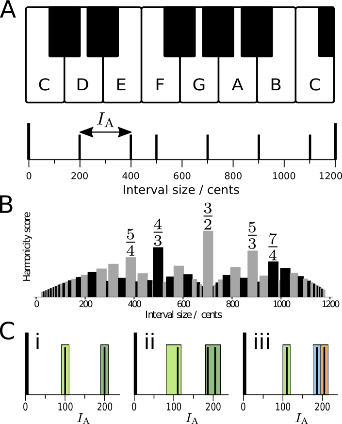
Figure 1: A: The major scale starting on a C shown on a piano (equal temperament), and as interval sizes (in cents) of each note measured from the first note. Intervals between adjacent pairs of notes are denoted by $I_{\textrm{A}}$. B: We use a harmonicity template to assign harmonicity scores to intervals [8]. The highest scoring intervals (frequency ratios are shown for the top five) act as windows of attraction, whereby any interval in this window is assigned its score. In this case the maximum window size is $w=40$ cents. C: Adjacent interval, $I_{\textrm{A}}$, sets for the major scale in equal temperament (i) and just intonation (ii & iii). Boxes indicate interval categories, where the width represents the error, and boxes with similar colours are related by a common denominator: (i) is losslessly compressed; a similar compression of (ii) is lossy; (iii) is uncompressed and therefore costs more to transmit.

Transmittability Model

The transmittability theory assumes that intervals are perceived as broad categories, and the humans make errors in both production and perception of intervals. Intervals must thus be large enough to avoid errors in transmission due overlapping interval categories (SI Fig. 1). This is not sufficient, however, to explain the considerable convergence in scales across cultures. We can further consider that scales are optimized for minimizing errors in transmission by favouring the use of large intervals, however this bias exclusively favours equidistant scales (SI pg. 4). While equidistant scales do exist [43, 44, 45, 46], they are a minority [47], so additional mechanisms are needed to explain the origin of scales.

When humans encode continuous audiovisual information such as speech, musical rhythm, brightness, or color, there is evidence that it is done efficiently [48, 49, 50, 51, 52, 53, 54]. If the same is true for pitch, then compressible scales would facilitate communication of melodies. An example of a compressible scale is the equal temperament major scale (Fig. 1A). We can represent this scale using its notes (C, D, etc.) or as a sequence of adjacent intervals, $I_{\textrm{A}}$: $200,200,100,200,200,200,100$. The most compressed representation uses an alphabet size of one by encoding the large interval ($200$) in terms of the small one ($100$) (Fig. 1Ci). However for the just intonation tuning – $I_{\textrm{A}}$: $204,182,112,204,182,204,112$ – this code is lossy (Fig. 1Cii). Lossless compression would require a three letter alphabet (Fig. 1Ciii).

With this in mind, we create a third model (TRANS) to test whether scales evolved to be compressible. We define scale compressibility as how accurately an $I_{\textrm{A}}$ set can be represented by a simple interval category template. We consider templates with categories centred about integer multiples of a common denominator (e.g., $100$, $200$, $300$). Accuracy in this case corresponds to the distance between $I_{\textrm{A}}$ and the centre of the closest category. Note that this is merely an approximation of information-theoretic compressibility as we do not explicitly calculate the information content. The TRANS model assumes that scales are selected for their ease of communication, and that this is captured by our measure of compressibility.

Generative Monte-Carlo simulations

To test the theories, we use Monte Carlo simulations to generate populations of scales, based on the above discussion on harmonicity and transmittability. We impose a minimum interval size constraint, $I_{\textrm{min}}$, such that scales with intervals $<I_{\textrm{min}}$ are rejected. Depending on the theory, we accept or reject scales according to a cost function and a corresponding Boltzmann probability, which allows us to control the strength of the bias via a parameter $\beta$. As $\beta$ increases, the generated populations become increasingly selective and eventually too selective, resulting in an optimal $\beta$ at which the generated scales best matches the empirical scales.

We examine and compare results for five models:

• RAN: random scales subject to no constraints or biases.

• MIN: random scales with a minimal interval constraint.

• FIF: scales that maximize the number of imperfect fifths.

• HAR: scales biased to have high harmonic similarity score.

• TRANS: transmittable scales biased to be compressible.

To simplify our simulations, we assume that adjacent intervals, $I_{\textrm{A}}$, in a scale add up to an octave of fixed size, $1200$ cents. We fix the number of notes, $N$, as a model parameter. In addition, (i) The FIF, HAR, and TRANS models are also subject to the $I_{\textrm{min}}$ constraint of the MIN model; (ii) The FIF and HAR models include the maximum window size $w$ as a variable parameter; (iii) The TRANS model has a single parameter, $n$, that affects the way inaccuracies due to compression are penalized.

For each model we generate a sample size of $S=10^{4}$ scales. Unless stated otherwise, we show results for $I_{\textrm{min}}$ = $80$ cents, $w=20$ and $n=2$. We varied the parameters $I_{\textrm{min}}$, $w$ and $n$, and found that differences are not negligible but do not alter the main results of this work (SI Fig. 2). We optimized the strength of the bias for each model and each $N$ by tuning $\beta$ (SI Table 4).

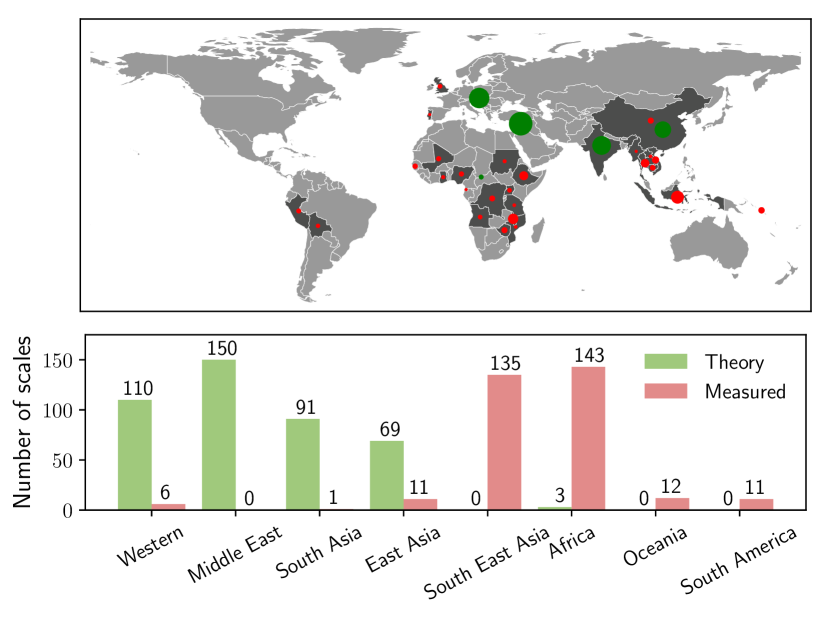
Figure 2: Scales in the database either come from a mathematical theory (theory) or from measurements from instruments or recordings (measured). The map shows the origin of the scales (theory: continents; measured: dark shaded countries), with sample size, $S$, indicated by the marker size.

Scale database

To evaluate the models, we created a database with the aim of recording the diversity of scales used by different cultures. To this end, we compiled scales that use exact mathematical ratios for interval sizes (e.g., Western, Arabic, Carnatic), taking into account usage of different tuning systems (e.g., equal temperament, just intonation) [12]. Despite the wealth of scales of this type, these cultures are but a fraction of the those that produce music. In our aim to obtain a comprehensive, diverse database we amalgamated work from ethnomusicologists who measured tuning systems used across the world. The database is split into ‘theory’ scales (sample size, $S=423$) which have exact theoretical values for frequency ratios, and ‘measured’ scales ($S=319$) which were inferred from measurements of instrument tunings and recorded performances (Fig. 2). ‘Measured’ scales within a culture can vary significantly (e.g., the Gamelan slendro scale), and given our goal of capturing this diversity, we recorded multiple ‘measured’ scales even if they have the same name. A full list of references, inclusion criteria, and the numbers/types of scales taken from each reference, are presented in the SI, Table 2 and 3.

A caveat with this approach is that the database might reflect hidden biases. For example, imperial dominance and globalization can result in homogenization of cultures [35], and many ethnomusicologists were biased towards reporting on cultures that were more distinct than similar [6]. It is therefore inherently difficult to rigorously define a ‘correct’ empirical distribution of scales, but we believe that this is a suitable approach to start with. Another issue is that despite the wide coverage of the database, it includes only a fraction of cultures, both geographically and historically, so it can be considered a lower bound on the diversity of scales. These limitations may be overcome with the aid of tools that can reliably estimate scales from ethnographic recordings, which will enable studies on a larger scale [28, 36]. By making our database open we hope to inspire others to plug these gaps and undertake further quantitative analysis of musical scales.

Packing intervals into octaves partially explains our choices of adjacent intervals

Adjacent intervals, $I_{\textrm{A}}$, can be considered the building blocks of scales. Many musical traditions use a restricted set of adjacent intervals with which multiple scales are formed. Fig. 3 shows $I_{\textrm{A}}$ histograms of database scales (DAT) for $N=4-9$ notes with the sample size, $S$, indicated. The $N=5$ and 7 note scales are most common [15]. However, we have few examples of 4 and 9 note scales, but nonetheless we have included them as they offer some information about the general shape of the distributions if not the details.

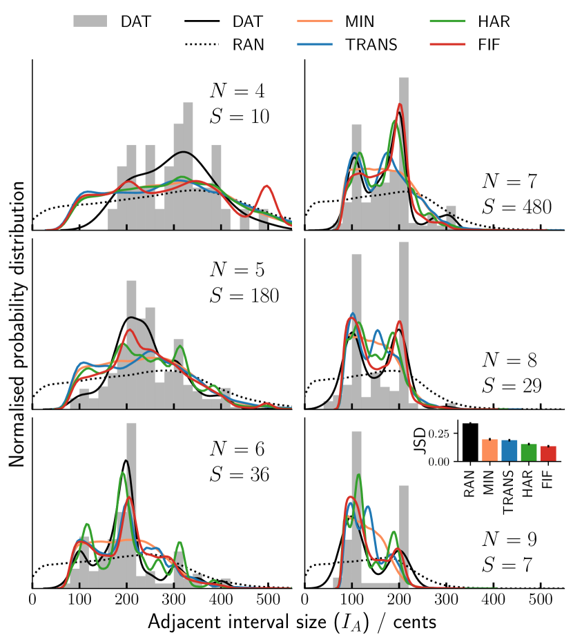
Figure 3: Adjacent interval ($I_{\textrm{A}}$) probability distributions for empirical DAT scales (black solid line) and model scales. The sum of the probabilities is one. Lines are fitted to histograms using kernel density estimation. Histograms (bin size is $20$ cents) and sample sizes ($S$) are shown only for DAT scales. Each panel shows the distributions for a given note number $N=4-9$. Inset: the average Jensen-Shannon divergence, JSD, between model and DAT distributions for each model; whiskers indicate $95\%$ confidence intervals.

The empirical distributions of the DAT scales, shown in Fig. 3, are clearly not random. Some intervals are more common, in particular a peak at 200 cents is prominent for all $N$. As $N$ increases, the main peaks in the distributions shift to the left (smaller interval sizes) and the range shrinks. This trend holds also for RAN scales, and by including the minimum interval constraint (MIN model), the ranges of the theoretically generated distributions approximate the empirical ones. This indicates that at the most basic level, the choice of intervals may be considered a packing problem. Given $N$ intervals of size $I_{\textrm{A}}$, their distribution depends on the possible ways that these $N$ intervals can be combined into an octave. Still, this description fails to explain the significant peaks and troughs in the distributions.

The FIF model best replicates empirical adjacent interval distributions

The models which use biases result in distributions with clear peaks and troughs (Fig. 3). In the TRANS distributions, some of the peaks are aligned with the DAT distributions ($N=6,7$), while others are clearly not ($N=8,9$). The existence of prominent peaks at $1200/N$, in addition to other peaks, indicates that the bias favours equidistant scales, but not exclusively. The HAR and FIF distributions match many of the features of the DAT distributions. The sample-size averaged Jensen-Shannon divergence between the DAT and the model distributions (Fig. 3 inset, SI Table 5) show that the FIF  model best fits the DAT distributions. This is somewhat unexpected, as the FIF model only specifies the inclusion of fifths, a large interval, while it predicts the distribution of smaller adjacent intervals. To explain the performance of the FIF model, we can consider how these building blocks are arranged into scales.

The FIF model best replicates the empirical note distributions

The MIN, and TRANS models accept or reject scales based only on their adjacent intervals, disregarding their order. Since the HAR and FIF models use all intervals (by comparing all pairs of notes) in their cost functions, they take the interval order into account. Hence, to see if interval order is indeed an important determinant, we examine how the notes are distributed in the scales (Fig. 4). Only $N=5$ and $N=7$ are shown due to the stricter need for sufficient statistics when considering the full scale distributions. The distributions of DAT scales show that certain notes are favoured, with notable peaks at 200, 500 and 700 cents for both $N$. Apart from exclusion zones at the boundaries, every note (when discretized in bins of width 30 cents) is used in at least one scale.

Among the models, the MIN distributions lack much detail beyond noise, apart from slight undulations with a periodicity of $\frac{1200}{N}$ cents. The TRANS distributions contain some notable peaks. Peaks at 500 and 700 cents fit the DAT distributions, while the 600 cents peak for $N=5$ is indubitably incorrect. The HAR and FIF distributions replicate the main features of the DAT distributions, including peaks, contour and troughs. The extra detail in the HAR model appears as additional peaks at harmonic intervals in the distributions.

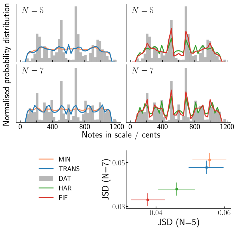
Figure 4: Top: Probability distribution of scale notes for DAT and model scales. Histograms are shown as lines for model results; sample sizes for DAT scales are the same as in Fig 3. Histograms (bin size is $30$ cents) are truncated at $15$ and $1185$ cents for clarity. Bottom: JSD between model and DAT distributions for $N=5$ and $N=7$; whiskers indicate $95\%$ confidence intervals.

Lacking rules for ordering intervals into scales, the TRANS model still performs well

We can compactly represent the performance of models by two scalar measurables (Fig. 5):

• The sample-size-weighted Jensen-Shannon divergence between DAT and theoretical $I_{\textrm{A}}$ distributions for each model.

• $f_{\textrm{D}}$ – The fraction of DAT scales that are found in the model-generated populations.

Due to our assumption that intervals in a scale add up to $1200$ cents, many ‘measured’ scales cannot be found by the model due to inexact octave tunings, resulting in an upper bound of $f_{\textrm{D}}\approx 0.8$. Additionally, the models generate samples of $S=10^{4}$ scales, and while JSD converges by this point, $f_{\textrm{D}}$ does not – i.e., as $S$ increases, so will $f_{\textrm{D}}$.

The TRANS model is better suited to predicting DAT scales than predicting DAT note distributions. This is surprising, given that the TRANS model offers no guidance on how to arrange intervals into a scale. Correlations between intervals in our database show that two intervals are usually ordered such that large goes with small and vice versa (we call this ‘well-mixed’). Two small (large) intervals are half as likely to be placed together in DAT scales than random chance would predict (SI Fig. 3). By shuffling the model scales with a bias towards mixing of sizes, we observed an average increase in $f_{\textrm{D}}$ of $12\%$ for the TRANS model while seeing an average decrease of $22\%$ for the FIF model (SI Fig. 4). So while scales tend to be arranged so that interval sizes are well-mixed, it is more important that they are arranged to maximise the number of fifths. Given that the FIF (HAR) and TRANS models are independent of each other, the performance of the TRANS model is quite notable.

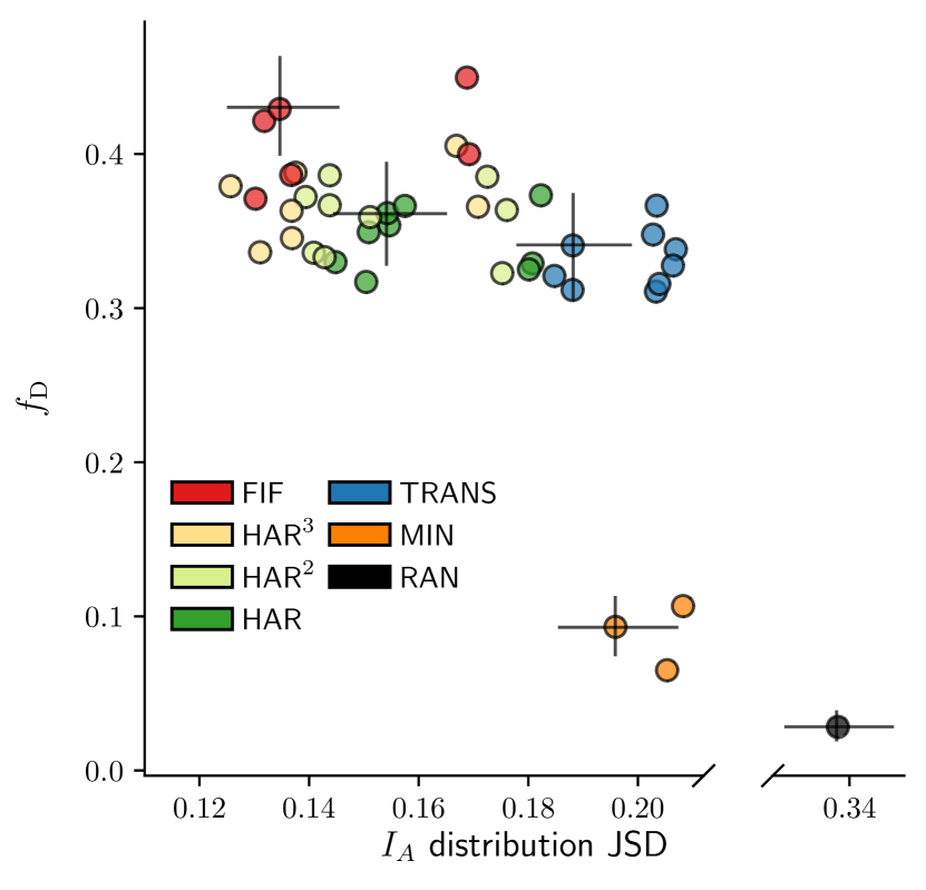
Figure 5: Model performance is plotted as the Jensen-Shannon divergence (JSD) between the DAT and model $I_{\textrm{A}}$ distributions against $f_{\textrm{D}}$, the fraction of DAT scales predicted. Superior models exhibit low JSD values and high values of $f_{\textrm{D}}$. Results for altered versions of the HAR model are also shown as HAR² and HAR³. For each model, results are shown for combinations of parameters: $I_{\textrm{min}}=[70,80,90]$, $w=[5,10,15,20]$, $n=[1,2,3]$, and in each case the bias strength $\beta$ is optimized. Whiskers indicating $95\%$ confidence intervals are only displayed for the models shown in Fig. 3, Fig. 4 and Fig. 6.

HAR model performance relies heavily on imperfect fifths

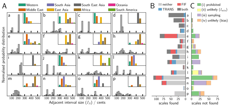
Figure 6: A: $I_{\textrm{A}}$ interval distributions of empirical DAT scales for clusters a-p and their geographical composition (inset). B: Number of DAT scales found by neither model, only the TRANS model, only the FIF model, or both models, for cluster a-p. C: For the scales that are not found by any of the TRANS, FIF, or HAR models, we show the breakdown of the reasons why: (i) prohibited due to model constraints, (ii) unlikely due to model constraints, (iii) insufficient sampling, (iv) unlikely due to model biases.

Despite the FIF model being a much simpler version of the HAR model, the FIF model achieves superior results according to our metrics (Fig. 5). To identify possible reasons, we interpolate between the HAR and FIF model templates by taking as a harmonicity score the $m$-th power of the harmonicity template in Fig. 1B, thereby approaching the FIF template as $m\to\infty$. Fig. 5 shows the results for models where we use $m=2$ (HAR²) and $m=3$ (HAR³), together with the original HAR model ($m=1$). The results indicate that as one interpolates from the HAR model to the FIF model the performance also interpolates continuously. Additionally, we note that the FIF and HAR models are strongly correlated (e.g., Pearson’s $r=0.76$ at $w=20$, SI Fig. 5B). This implies that fifths are a dominant part of the HAR model, while the extra detail merely hinders performance.

Clustering of scales reveals differences between model predictions

To further understand how the models work, and in particular why two disparate theories (harmonicity and transmittability) perform well, we examined what types of DAT scales they predict. We divide the scales into 16 clusters by hierarchical clustering based on their $I_{\textrm{A}}$ sets. In Fig. 6A we display the $I_{\textrm{A}}$ distribution and geographical composition for each cluster. Middle Eastern, Western, South Asian and East Asian scales appear to have been at one time based on similar mathematics [55, 56, 57, 58, 12], so it might be expected that they should cluster together (a, c, j, l). There are similarities between some South East Asian and African cultures that utilise equidistant 5 and 7-note scales (d, h, i, p). Clearly there are also some clusters that might be ill-defined (e, k).

The number of scales in each cluster found by the TRANS and FIF models is shown in Fig. 6B. For clarity, we omit the HAR results as they are qualitatively similar to the FIF results, but with less scales predicted (SI Fig 6A). The conclusions drawn about the differences between the TRANS and FIF models are also relevant when comparing the TRANS and HAR models. All models appear to perform well when $I_{\textrm{A}}$ distributions are uni/bimodal with sharp peaks (a, b, c, i). The TRANS model performs better if $I_{\textrm{A}}$ distributions have sharp peaks, regardless of how many peaks there are (a, c, d, i, j, l). The harmonicity models are better adapted to scales from clusters with broad $I_{\textrm{A}}$ distributions (b, e, f, g, h, m, n). Despite these differences, the majority of scales that are found are common to all models, and while the TRANS and FIF (HAR) cost functions are not correlated in MIN scales (Pearson’s $r=0.01$ ($-0.04$)) they are correlated in DAT scales (Pearson’s $r=0.41$ ($0.12$)) (SI Fig 7). Ultimately, of those scales that are predicted, a majority appear to be selected for both harmonicity and transmittability.

A majority of scales were predicted by at least one model

Between the three models, $407$ out of $742$ ($55\%$) scales were found. There are several reasons why the other scales were not found: (i) It is impossible for the model to generate them due to having an interval smaller than $I_{\textrm{min}}$ or deviations from a perfect octave. (ii) It is possible but unlikely for the model to generate them due to having intervals at the tails of the $I_{\textrm{A}}$ distributions - this is a feature of the random sampling, which is compounded by the use of an $I_{\textrm{min}}$ constraint. (iii) They are likely to be found, but we generated too few samples to find them all. (iv) They are not likely to be found by any model.

We calculated the breakdown of the reasons why scales were not found (Fig. 6C). Scales are in category (i) if $I_{\textrm{min}}<70$ or if the octave deviates from $1200$ cents by more than $10$ cents ($155$ scales). For all scales we calculate the probability, $P_{\textsc{MIN}}$, that they are predicted after applying the $I_{\textrm{min}}$ constraint, and note the value of $P_{\textsc{MIN}}$ below which only $10\%$ of scales are not found. Scales with $P_{\textsc{MIN}}$ lower than this value are in category (ii) ($26$ scales), or in one of categories (iii) and (iv) otherwise. We calculate for all scales the probability, $P_{\textsc{ANY}}$, that a scale will be found by any model, and note the value of $P_{\textsc{ANY}}$ below which only $10\%$ of scales are not found. Scales with $P_{\textsc{ANY}}$ higher than this value are in category (iii) ($100$ scales), otherwise (iv) ($54$ scales). When we only consider scales that the model can predict (categories ii-iv), we find that the three models are not particularly sensitive to ‘theory’ or ‘measured’ scales, nor the region or culture from which they come (SI Fig 6). This implies that these biases are in effect consistently across musical traditions.

Discussion

Packing arguments account for the success of the harmonicity models

The FIF model manages to reproduce the main features of the interval ($I_{\textrm{A}}$) and scale distributions, simply by specifying inclusion of fifths. This may seem counter-intuitive, but it can be rationalised entirely in terms of packing. Consider first Fig. 4. Since $0$ and $1200$ cents are fixed points, the easiest way to add fifths is by having notes at $500$ ($1700$) or $700$ cents. Taking into account the circular nature of scales, one can subsequently add notes at $200$ ($1400$) cents or $1000$ cents, which will further interact with previously added notes to create more fifths. As a result, there are exclusion zones at either side of $500$ and $700$ cents. Packing also explains the features of the $I_{\textrm{A}}$ distributions in Fig. 3: if $200$, $500$, $700$ and $1000$ cents are all highly probable, then the $I_{\textrm{A}}$ distributions ought to contain many $200$ cents intervals regardless of $N$.

It is likely that packing is also the main mechanism in the HAR model. The HAR model is affected not only by the harmonic template (Fig. 1B), but also the constraints of fixed $N$ and octave size. The HAR results then arise from the ways of arranging a scale to maximize its average harmonicity score. The fifth is the most important interval in the HAR model, as evidenced by its high score and also the high correlation between the FIF and HAR cost functions (SI Fig 5B). The similarities between the FIF and HAR results (Fig. 3, 4 and SI Fig. 6A) provides additional evidence that the HAR model shares the FIF packing mechanism. Constructing scales from fifths is an old concept [11]. The new understanding is that different cultures can be explained in this way even when there is no evidence that they explicitly tuned instruments using fifths (SI Fig. 6).

The devil in music? – The devil is in the detail

The tritone interval (${\sim}600$ cents) has been traditionally considered dissonant in Western music – earning it the name diabolus in musica [59] – and is uncommon in classical and folk music [60]. Is it rare because it is unpleasant, or unpleasant because it is rare? Viewing scales as a packing problem reveals an alternative explanation: as $N$ increases, the average $I_{\textrm{A}}$ size decreases, and it becomes easier to simultaneously pack both tritones and fifths. Analysis of the database shows a linear relationship between $N$ and the frequency of tritone intervals, and this trend is replicated best by the FIF model (SI Fig. 8). Therefore according to this theory, the tritone is rarely used in music simply because it is difficult to simultaneously pack tritones and fifths.

On the universality of harmonic intervals

The oft-repeated claim that harmonic intervals are universal is based on sparse statistical evidence [59]. Our data shows that harmonicity and prevalence are correlated, and this correlation depends on $N$ ($N=5$, $r=0.70$, $p<0.005$; $N=6$, $r=0.43$, $p>0.05$; $N=7$, $r=0.65$, $p<0.005$; SI Fig. 9). Fifths ($3/2$, $702$ cents) and, due to inversion, fourths ($3/2$, $498$ cents) are the most widespread. However the ratios $7/6$ ($267$ cents) and $7/4$ ($968$ cents) are quite rare despite their relatively high harmonicity, in contrast to $11/7$ ($783$ cents) which is more common yet less harmonic. Thus we report the first clear evidence for prevalence of harmonic intervals, showing that the correlation between prevalence and harmonicity is not straightforward.

Multiple selection pressures affect evolution of scales

All three models, HAR, FIF and TRANS, explain the empirical data significantly better than chance. Thus it is possible that scales are simultaneously optimized for compressibility, maximization of fifths, and maximization of other harmonic intervals. Out of the two harmonicity models, the FIF model better fits the data than the HAR model, but we note that these models are the two extreme cases in how they treat higher order harmonics. A more sophisticated model may have a nuanced approach that accounts for the spectra of natural sounds and how they are processed. There is also a speculative scenario in which harmonic intervals are selected through a different mechanism. The cultures which use small-integer frequency ratios (‘theory’ scales) overlap with those that had contributed to the development of mathematics [61]. Thus the use of mathematics may have contributed to the development of scales [62].

A significant minority of scales are not supported by any model. A view some may consider natural is that perhaps no one mathematical model can predict the diversity of scales. Regarding the theories tested: cultures which produce monophonic music may ignore harmony [19]; cultures which primarily focus on rhythm and dance may not mind imprecision in melodies. Consider the Gamelan pelog scale, variations of which account for over two thirds of cluster p. Pelog scales rarely contain imperfect fifths (SI Fig. 10A). A crude approximation of the pelog scale reduces it to intervals on a 9-TET (9-tone equal temperament) scale [63]. This scale is composed of 5 small intervals (average size 133 cents) and 2 large intervals (average size 267 cents). This should be predicted by the TRANS model, but within individual pelog scales the deviations from 9-TET are so large that this rarely happens.

The pelog scale is not exceptional in this regard; huge deviations from the average are seen in Thai scales and the Gamelan slendro scale (SI Fig. 10). In this case, some propose that the deviations from some mathematical ideal are not examples of mistuning, but rather a display of artistic intent [64, 65, 66]. Tuning as a means of expression is rare in the West, but not unheard of in classical or popular music (see La Monte Young’s ”The Well-tuned Piano” or King Gizzard and the Wizard Lizard’s ”Flying Microtonal Banana”). While these theories have performed well, the variability in scales of some cultures hints that although scales are inherently mathematical, mathematics alone lacks the power to fully explain our choices of scales.

Limitations due to assumptions and data

We report that the FIF model best fits the available data, and we assume that the data is representative of scales used in different musical traditions. However, a different data collection method may significantly alter the results. We replicated the analysis with sub-samples of our database and found that the conclusions are at least robust to resampling (SI Fig 11). Future work may benefit from controlling for historical relationships between musical traditions [47].

Despite evidence that tonal hierarchies are common, they are not a necessary element of scales so we avoid assumptions about tonality [2, 67]. We could have assumed that the tonic (the note at $0$ cents) is special, and so are intervals made with the tonic. This would explain why in Fig. 4 the $700$ cents is more salient than $500$ cents. We note that the we could have chosen a different proxy measure of harmonicity [39]. However, we think that doing so would not alter the conclusions as the different measures are highly correlated (SI Fig 5A).

Lack of hexatonic scales may be owing to historical convention

Why do we choose $N$ notes in a scale? – It is generally agreed that there is some trade-off involved. With too few notes melodies lack complexity; with too many notes melodies are difficult to learn. Too few notes results in larger intervals which are more difficult to sing [68]; too many notes results in smaller intervals which have lower harmonic similarity [8]. This simple trade-off is at odds with the contrasting ubiquity of 5 and 7 note scales and scarcity of 6 note scales. One suggestion is that 6 note scales are actually prevalent, but classified as variants of 5 and 7 note scales due to convention. Evidence for this can be found in the Essen folk song collection [69].

Chinese music and Western music are conventionally thought to be composed using 5 and 7 note scales respectively, but for both cultures, 6 note scales are the second most prevalent in folk songs (SI Fig. 12). While the following is mere speculation, this work points to a possible route by which a preference for pentatonic and heptatonic scales may have arisen. Given the simplicity of equidistant scales, they are the easiest compressible scales to evolve. For 5, 6, 7 and 8 note equidistant scales, the closest notes to fifths are 720 cents, 600 (800) cents, 686 cents, and 750 cents, respectively. Thus, 5 and 7 note scales are the only equidistant scales that can include imperfect fifths. The paucity of recorded hexatonic scales may therefore be due to historical convention driven by evolutionary pressures in early music.

Conclusion

By constructing a cross-cultural database and using generative stochastic modelling, we quantitatively tested several theories on the origin of scales. Scales tend to include imperfect fifths, and the features of the empirical distributions arise from the most probable ways of packing fifths into a scale of fixed length. Scales also tend to be compressible, which we suggest leads to melodies that are easier to communicate and remember. There is evidence that efficient data compression is a general mechanism humans use for discretizing continuous signals. The effect of compressibility on pitch processing merits further research.

No single theory could explain the diversity exhibited in the database. It is instead likely that scales evolved subject to different selection pressures across cultures. These theories can be further tested by expanding the database, in particular by computationally identifying scales used in ethnographic recordings. Out of two harmonicity-based theories, the one that best fits the empirical data only considers the first three harmonics. This may shed some light on the important, but still developing, understanding of how harmonicity is processed in the brain.

Methods

The stochastic models

The stochastic models generate adjacent intervals $I_{\textrm{A}}$ from a uniform distribution, which are then scaled so that they sum to $1200$ cents. Some models apply a minimum interval constraint, $I_{\textrm{min}}$, such that no $I_{\textrm{A}}$ is smaller than $I_{\textrm{min}}$. Depending on the model, scales are accepted or rejected according to a probability

$$P=\min\left\{1,\exp(-\beta C)\right\}~{},$$ (1)

where $C$ is a cost function, and we tune the strength of the bias with the parameter $\beta$. We tested many cost functions to check that the results are insensitive to the exact functional form (SI Fig. 13, 14, 15).

For the harmonicity model HAR,

$$C_{\textsc{HAR}}=1-\frac{\bar{H}-\bar{H}_{min}}{\bar{H}_{max}-\bar{H}_{min}}~{},$$ (2)

where $\bar{H}_{min}$ and $\bar{H}_{max}$ are normalization constants (these constants, obtained via random sampling, are listed in SI Table 4), and the average harmonicity score $\bar{H}$ is given by

$$\bar{H}=\bigg{[}N(N-1)\bigg{]}^{-1}\sum^{N-1}_{i=0}\sum^{i+N-1}_{j=i+1}H(I_{ij},w)~{},$$ (3)

where $H(I)$ is the harmonic similarity score of an interval size $I$, $w$ is the size of the window in which intervals are considered equivalent, and $I_{ij}$ is the interval between note $i$ and note $j$. The index $i=0$ refers to the starting note of the scale and $j$ takes into account the circular nature of scales (if $j>N$ then note $j$ is an octave higher than note $j-N$). Note that we do not consider either unison or octave intervals in this score. The harmonic similarity score $H$ of an interval is calculated from its frequency ratio expressed as a fraction.

$$H(I)=\frac{x+y-1}{xy}\times 100~{},$$ (4)

where $x$ is the numerator and $y$ is the denominator of the fraction. The harmonic similarity template is produced by creating a grid of windows of maximum size $w$ centred about the intervals that have the largest $H$ values. An interval expressed in cents is allocated to the window with the highest $H$ value that is within $w/2$ cents.

For the imperfect fifths model FIF,

$$C_{\textsc{FIF}}=(1+\bar{F})^{-1}~{},$$ (5)

where a constant is added to prevent division by zero in the case of scales with no imperfect fifths, and the fraction of fifths $\bar{F}$ is

$$\bar{F}=\bigg{[}N(N-1)\bigg{]}^{-1}\sum^{N-1}_{i=0}\sum^{i+N-1}_{j=i+1}F(I_{ij},w)~{},$$ (6)

where $F(I,w)=1$ if $|I-702|\leq w/2$ and $0$ otherwise.

For the transmittable scales model TRANS,

$$C_{\textsc{TRANS}}=\min_{\frac{1}{2}\min\{I_{\textrm{A}}\}\leq\gamma\leq\frac{3}{2}\min\{I_{\textrm{A}}\}}\left\{\sum^{N}_{i=1}\Bigg{|}\left\lceil\frac{I_{Ai}}{\gamma}\right\rceil-\frac{I_{Ai}}{\gamma}\Bigg{|}^{n}\right\}/N~{},$$ (7)

where $I_{Ai}$ is the $i^{\rm th}$ adjacent interval in a scale, and $n$ is parameter that controls how deviations from the template are considered in the model (see main text). The parameter $\gamma$ is the common denominator of the compressible template; it is constrained so that it is never less than half of the smallest adjacent interval.

Classification of scales as similar

The fraction of DAT scales $f_{\textrm{D}}$ for each model was calculated by checking if model scales are similar to DAT scales. Two scales A and B are similar if

$$\forall i\in\{1..N\},|\alpha^{A}_{i}-\alpha^{B}_{i}|\leq e~{},$$ (8)

where $\alpha^{A}_{i}$ is $i^{th}$ note in scale $A$ and the tolerance is $e=10$.

Probability of predicting scales

$P_{\textsc{MIN}}$, the probability of a scale A being predicted by the MIN model, is calculated as the sum of the probabilities of each scale $B$ that can be labelled similar to, or the same as, scale $A$. We use a tolerance of $e=10$, we keep the length of the scale constant, and we consider probabilities at an integer resolution, so there are $21^{N-1}$ similar scales.

$$P_{\textsc{MIN}}=\sum^{21^{N-1}}\prod^{N}_{i=1}p(I^{B}_{\textrm{A}i})~{},$$ (9)

where $p$ is the probability of an interval being picked by the MIN model, and $I^{B}_{\textrm{A}i}$ is the $i^{th}$ adjacent interval in scale B.

$P_{\textsc{ANY}}$, the probability that any of the TRANS, HAR or FIF models finds a scale is given by

$$P_{\textsc{ANY}}=P_{\textsc{MIN}}\sum P(\beta,C)~{},$$ (10)

where $P$ is summed over the three models using the parameters listed in SI Table 4.

Clustering criterion

To group DAT scales we used hierarchical clustering based on distances between adjacent intervals. The distance, $d_{AB}$, from scale $A$ to scale $B$ is asymmetric, and is calculated as the sum of the shortest distances from every $I_{\textrm{A}}$ in $A$ to any $I_{\textrm{A}}$ in B,

$$d_{AB}=\sum_{i=1}^{N}\min_{j}\{I^{A}_{\textrm{A}i}-I^{B}_{\textrm{A}j}\}~{},$$ (11)

where $i$ and $j$ are the indices of adjacent intervals in scales $A$ and $B$ respectively. For clustering, we use the symmetric distance $d_{C}=(d_{AB}d_{BA})^{1/2}$. We used Ward’s minimum variance method to agglomerate clusters using the SciPy package for Python [70].

Statistical analysis

We tested whether the empirical $I_{\textrm{A}}$ and note distributions are better approximated by a theoretical model (FIF,HAR,TRANS), compared to the RAN, and the MIN model, which are effectively the null distributions. We chose to smooth the $I_{\textrm{A}}$ distributions in Fig. 3 mainly due to one assumption. Given that (with the exception of modern fixed pitch instruments) intervals are not produced as exact frequency ratios, the $I_{\textrm{A}}$ distributions should be smooth. We consider that the sharp peaks (e.g., at $100$ and $200$ cents are a result of theoretical values for interval sizes and are not representative of how intervals are produced in reality. To minimize artefacts from this smoothing we used a non-parametric kernel density estimation method, implemented in the Statsmodels package for Python [71]. The kernel is Gaussian and Silverman’s rule is used to estimate the bandwidth. We compared goodness-of-fit between the empirical and theoretical distributions using the Jensen-Shannon divergence (we get the arithmetic mean across $N$, weighted by sample size). We verified that the smoothing did not influence the results by using a two sample Cramér-von Mises test (SI Table 5). Due to the high dimensionality of the system we needed to generate large samples ($S=10^{4}$) for each model. As a result, $p$ values tend to be astronomically low ($p\ll 0.01$), so we instead calculated $95\%$ confidence intervals by bootstrapping (1000 resamples from the DAT sample). Applying kernel density estimation to the note distributions (Fig. 4) resulted in a loss of detail via oversmoothing. Hence, we only show histograms for these distributions and calculate the Jensen-Shannon divergence using the histograms. The conclusions do not depend on the histogram bin size. To test whether we have sufficient empirical data we replicate the analysis with three types of sub-sampling: bootstrapping with smaller sample sizes; only the ‘theory’ scales; and only the ‘measured’ scales (SI Fig 11). We find that the conclusions are robust to resampling.

Data and Code Availability

All data used in the figures and Supplementary Information are available, along with simulation and analysis code are accessible at https://github.com/jomimc/imperfect_fifths. The scales database is included as Supplementary Material.

Acknowledgements

J.M. acknowledges helpful discussions with Patrick Savage. This work was supported by the taxpayers of South Korea through the Institute for Basic Science, Project Code IBS-R020-D1.

Competing Interests

The authors declare that they have no competing financial interests.

Correspondence

Correspondence and requests for materials should be addressed to J.M. (email: jmmcbride@protonmail.com) and T.T. (tsvitlusty@gmail.com).

Author Contributions

J.M. and T.T. designed research; J.M. performed research; J.M. analyzed data; J.M. and T.T. wrote the paper.

References

- Darwin [1896] C. Darwin. The Descent of Man and Selection in Relation to Sex, volume 1. D. Appleton, 1896.
- McDermott and Hauser [2005] J. McDermott and M. Hauser. The origins of music: Innateness, uniqueness, and evolution. Music Percept., 23(1):29–59, 2005. 10.1525/mp.2005.23.1.29.
- Fitch [2006] W. T. Fitch. The biology and evolution of music: A comparative perspective. Cognition, 100(1):173 – 215, 2006. https://doi.org/10.1016/j.cognition.2005.11.009.
- Ball [2010] P. Ball. The Music Instinct: How Music Works and Why We Can’t Do Without It. Random House, 2010.
- Wallin et al. [2001] N. L. Wallin, B. Merker, and S. Brown. The Origins of Music. MIT press, 2001.
- Nettl [2010] B. Nettl. The Study of Ethnomusicology: Thirty-One Issues and Concepts. University of Illinois Press, 2010.
- Brown and Jordania [2013] Steven Brown and Joseph Jordania. Universals in the world’s musics. Psychol. Music, 41(2):229–248, 2013. 10.1177/0305735611425896.
- Gill and Purves [2009] K. Z. Gill and D. Purves. A biological rationale for musical scales. Plos One, 4(12):1–9, 2009. 10.1371/journal.pone.0008144.
- Schwartz et al. [2003] D. A. Schwartz, C. Q. Howe, and D. Purves. The statistical structure of human speech sounds predicts musical universals. J. Neurosci., 23(18):7160–7168, 2003. 10.1523/JNEUROSCI.23-18-07160.2003.
- Bruckert et al. [2010] Laetitia Bruckert, Patricia Bestelmeyer, Marianne Latinus, Julien Rouger, Ian Charest, Guillaume A. Rousselet, Hideki Kawahara, and Pascal Belin. Vocal attractiveness increases by averaging. Curr. Biol., 20(2):116 – 120, 2010. https://doi.org/10.1016/j.cub.2009.11.034.
- West [1994] M. L. West. The babylonian musical notation and the hurrian melodic texts. Music Lett., 75(2):161–179, 1994. 10.2307/737674.
- Rechberger [2018] H. Rechberger. Scales and Modes Around the World: The Complete Guide to the Scales and Modes of the World. Fennica Gehrman Ltd., 2018.
- Kuroyanagi et al. [2019] J. Kuroyanagi, S. Sato, M. J. Ho, G. Chiba, J. Six, P. Pfordresher, A. Tierney, S. Fujii, and P. Savage. Automatic comparison of human music, speech, and bird song suggests uniqueness of human scales. In Proceedings of the Folk Music Analysis (FMA 2019), 2019.
- Burns [1999] E. M. Burns. Intervals, scales, and tuning. In Diana Deutsch, editor, The Psychology of Music (Second Edition), pages 215 – 264. Academic Press, San Diego, second edition edition, 1999. https://doi.org/10.1016/B978-012213564-4/50008-1.
- Patel [2010] A. D. Patel. Music, Language, and the Brain. Oxford university press, 2010.
- McDermott et al. [2010a] Josh H. McDermott, Andriana J. Lehr, and Andrew J. Oxenham. Individual differences reveal the basis of consonance. Curr. Biol., 20(11):1035 – 1041, 2010a. https://doi.org/10.1016/j.cub.2010.04.019.
- Cousineau et al. [2012] M. Cousineau, J. H. McDermott, and I. Peretz. The basis of musical consonance as revealed by congenital amusia. P. Natl. Acad. Sci. Usa., 109(48):19858–19863, 2012. 10.1073/pnas.1207989109.
- Bowling and Purves [2015] D. L. Bowling and D. Purves. A biological rationale for musical consonance. P. Natl. Acad. Sci. Usa., 112(36):11155–11160, 2015. 10.1073/pnas.1505768112.
- McDermott et al. [2016] J. H. McDermott, A. F. Schultz, E. A. Undurraga, and R. A. Godoy. Indifference to dissonance in native amazonians reveals cultural variation in music perception. Nature, 535:547 EP –, 2016. 10.1038/nature18635.
- Jacoby et al. [2019] Nori Jacoby, Eduardo A. Undurraga, Malinda J. McPherson, Joaquín Valdés, Tomás Ossandón, and Josh H. McDermott. Universal and non-universal features of musical pitch perception revealed by singing. Curr. Biol., 2019. 10.1016/j.cub.2019.08.020.
- Savage [2019] P. E. Savage. The Need for Global Studies. Oxford University Press, New York, 2019.
- Pfordresher and Brown [2017] Peter Q. Pfordresher and Steven Brown. Vocal mistuning reveals the origin of musical scales. Eur. J. Cogn. Psychol., 29(1):35–52, 2017. 10.1080/20445911.2015.1132024.
- Sato et al. [2019] S. Sato, J. Six, P. Pfordresher, S. Fujii, and P. Savage. Automatic comparison of global children’s and adult songs supports a sensorimotor hypothesis for the origin of musical scales. In 9th Folk Music Analysis Conference, 2019. https://doi.org/10.31234/osf.io/kt7py.
- Siegel and Siegel [1977] J. A. Siegel and W. Siegel. Categorical perception of tonal intervals: Musicians can’t tell sharp from flat. Percept. Psychophys., 21(5):399–407, 1977. 10.1037/h0094008.
- Burns and Ward [1978] E. M. Burns and W. D. Ward. Categorical perception—phenomenon or epiphenomenon: Evidence from experiments in the perception of melodic musical intervals. J. Acoust. Soc. Am., 63(2):456–468, 1978. 10.1121/1.381737.
- Lynch et al. [1991] M. P. Lynch, R. E. Eilers, D. K. Oller, R. C. Urbano, and P. Wilson. Influences of acculturation and musical sophistication on perception of musical interval patterns. J. Exp. Psychol. Human., 17(4):967, 1991. 10.1037/0096-1523.17.4.967.
- McDermott et al. [2010b] J. H. McDermott, M. V. Keebler, C. Micheyl, and A. J. Oxenham. Musical intervals and relative pitch: Frequency resolution, not interval resolution, is special. J. Acoust. Soc. Am., 128(4):1943–1951, 2010b. 10.1121/1.3478785.
- Serra et al. [2011] J. Serra, G. K. Koduri, M. Miron, and X. Serra. Assessing the tuning of sung indian classical music. In ISMIR, pages 157–162, 2011.
- Devaney et al. [2011] J. Devaney, M. I. Mandel, D. P. W. Ellis, and I. Fujinaga. Automatically extracting performance data from recordings of trained singers. PsychoMusicology, 21(1-2):108, 2011. 10.1037/h0094008.
- Russo and Thompson [2005a] F. A. Russo and W. F. Thompson. An interval size illusion: The influence of timbre on the perceived size of melodic intervals. Percept. Psychophys., 67(4):559–568, 2005a. 10.3758/BF03193514.
- Russo and Thompson [2005b] F. A. Russo and W. F. Thompson. The subjective size of melodic intervals over a two-octave range. Psychon. B. Rev., 12(6):1068–1075, 2005b. 10.3758/BF03206445.
- Aruffo et al. [2014] C. Aruffo, R. L. Goldstone, and D. J. D. Earn. Absolute judgment of musical interval width. Music Percept., 32(2):186–200, 2014. 10.1525/mp.2014.32.2.186.
- Geringer et al. [2015] John M. Geringer, Rebecca B. MacLeod, and Justine K. Sasanfar. In tune or out of tune: Are different instruments and voice heard differently? J. Res. Music Educ., 63(1):89–101, 2015. 10.1177/0022429415572025.
- Larrouy-Maestri et al. [2019] P. Larrouy-Maestri, P. M. C. Harrison, and D. Müllensiefen. The mistuning perception test: A new measurement instrument. Behav. Res. Methods, 51(2):663–675, 2019. 10.3758/s13428-019-01225-1.
- Cowen [2009] T. Cowen. Creative Destruction: How Globalization Is Changing the World’s Cultures. Princeton University Press, 2009.
- Six and Cornelis [2011] J. Six and O. Cornelis. Tarsos: A platform to explore pitch scales in non-western and western music. In 12th International Society for Music Information Retrieval Conference (ISMIR-2011), pages 169–174, 2011.
- Plomp [1964] R. Plomp. The ear as a frequency analyzer. J. Acoust. Soc. Am., 36(9):1628–1636, 1964. 10.1121/1.1919256.
- Plack and Oxenham [2005] C. J. Plack and A. J. Oxenham. The psychophysics of pitch. In Pitch, pages 7–55. Springer, 2005.
- Harrison and Pearce [2019] P. Harrison and M. Pearce. Simultaneous consonance in music perception and composition. Psychol. Rev., 2019.
- Hartmann [1993] W. M. Hartmann. On the origin of the enlarged melodic octave. J. Acoust. Soc. Am., 93(6):3400–3409, 1993. 10.1121/1.405695.
- Loosen [1995] F. Loosen. The effect of musical experience on the conception of accurate tuning. Music Percept., 12(3):291–306, 1995. 10.2307/40286185.
- Carterette and Kendall [1994] Edward C. Carterette and Roger A. Kendall. On the tuning and stretched octave of javanese gamelans. Leonardo Music J., 4:59–68, 1994. 10.2307/1513182.
- Wachsmann [1950] K. P. Wachsmann. An equal-stepped tuning in a ganda harp. Nature, 165(4184):40–41, 1950. 10.1038/165040a0.
- Van Zanten [1980] W. Van Zanten. The equidistant heptatonic scale of the asena in malawi. Afr. Music, 6(1):107–125, 1980. 10.21504/amj.v6i1.1099.
- McNeil and Mitran [2008] L. E. McNeil and S. Mitran. Vibrational frequencies and tuning of the african mbira. J. Acoust. Soc. Am., 123(2):1169–1178, 2008. 10.1121/1.2828063.
- Ross and Knight [2017] Barry Ross and Sarah Knight. Reports of equitonic scale systems in african musical traditions and their implications for cognitive models of pitch organization. Music. Sci., page 1029864917736105, 2017. 10.1177/1029864917736105.
- Savage et al. [2015] P. E. Savage, S. Brown, E. Sakai, and T. E. Currie. Statistical universals reveal the structures and functions of human music. P. Natl. Acad. Sci. Usa., 112(29):8987–8992, 2015. 10.1073/pnas.1414495112.
- Lewicki [2002] M. S. Lewicki. Efficient coding of natural sounds. Nat. Neurosci., 5(4):356–363, 2002. 10.1038/nn831.
- Desain and Honing [2003] Peter Desain and Henkjan Honing. The formation of rhythmic categories and metric priming. Perception, 32(3):341–365, 2003. 10.1068/p3370.
- Ravignani et al. [2016] A. Ravignani, T. Delgado, and S. Kirby. Musical evolution in the lab exhibits rhythmic universals. Nature Human Behaviour, 1:0007 EP –, 2016. 10.1038/s41562-016-0007.
- Jacoby and McDermott [2017] Nori Jacoby and Josh H. McDermott. Integer ratio priors on musical rhythm revealed cross-culturally by iterated reproduction. Curr. Biol., 27(3):359 – 370, 2017. https://doi.org/10.1016/j.cub.2016.12.031.
- Stilp and Kluender [2010] C. E. Stilp and K. R. Kluender. Cochlea-scaled entropy, not consonants, vowels, or time, best predicts speech intelligibility. P. Natl. Acad. Sci. Usa., 107(27):12387–12392, 2010. 10.1073/pnas.0913625107.
- Regier et al. [2007] T. Regier, P. Kay, and N. Khetarpal. Color naming reflects optimal partitions of color space. P. Natl. Acad. Sci. Usa., 104(4):1436–1441, 2007. 10.1073/pnas.0610341104.
- Baddeley and Attewell [2009] Roland Baddeley and David Attewell. The relationship between language and the environment: Information theory shows why we have only three lightness terms. Psychol. Sci., 20(9):1100–1107, 2009. 10.1111/j.1467-9280.2009.02412.x.
- te Nijenhuis [1970] E. te Nijenhuis. Dattilam: A Compendium of Ancient Indian Music, volume 11. Brill Archive, 1970.
- Signell [1977] K. L. Signell. Makam: Modal Practice in Turkish Art Music, volume 4. Da Capo Pr, 1977.
- Farhat [2004] H. Farhat. The Dastgah Concept in Persian Music. Cambridge University Press, 2004.
- Katz [2015] I. Katz. Henry George Farmer and the First International Congress of Arab Music (Cairo 1932). Brill, 2015.
- Trehub [2018] S. E. Trehub. Human processing predispositions and musical universals. In Henkjan Honing, editor, The origins of musicality. The MIT Press, 2018.
- Vos and Troost [1989] P. G. Vos and J. M. Troost. Ascending and descending melodic intervals: Statistical findings and their perceptual relevance. Music Percept., 6(4):383–396, 1989. 10.2307/40285439.
- Goodman [2016] M. K. J. Goodman. An Introduction to the Early Development of Mathematics. John Wiley & Sons, 2016.
- Crocker [1963] Richard L. Crocker. Pythagorean mathematics and music. The Journal of Aesthetics and Art Criticism, 22(2):189–198, 1963. 10.2307/427754.
- Rahn [1978] Jay Rahn. Javanese pélog tunings reconsidered. Yearb. Int. Folk Music Council, 10:69–82, 1978. 10.2307/767348.
- Vetter [1989] Roger Vetter. A retrospect on a century of gamelan tone measurements. Ethnomusicology, 33(2):217–227, 1989. 10.2307/924396.
- Marcus [1993] S. Marcus. The interface between theory and practice: Intonation in arab music. Asian Music, 24(2):39–58, 1993. 10.2307/834466.
- Garzoli [2015] J. Garzoli. The myth of equidistance in thai tuning. Anal Approaches Music, 4(2):1–29, 2015.
- Kessler et al. [1984] E. J. Kessler, C. Hansen, and R. N. Shepard. Tonal schemata in the perception of music in bali and in the west. Music Percept., 2(2):131–165, 1984. 10.2307/40285289.
- Sundberg et al. [1993] J. Sundberg, I. Titze, and R. Scherer. Phonatory control in male singing: A study of the effects of subglottal pressure, fundamental frequency, and mode of phonation on the voice source. J. Voice, 7(1):15 – 29, 1993. https://doi.org/10.1016/S0892-1997(05)80108-0.
- Schaffrath [1995] H. Schaffrath. The essen folksong collection, 1995.
- Jones et al. [2001–] Eric Jones, Travis Oliphant, Pearu Peterson, et al. Scipy: Open source scientific tools for Python, 2001–.
- Seabold and Perktold [2010] S. Seabold and J. Perktold. Statsmodels: Econometric and statistical modeling with python. In 9th Python in Science Conference, 2010.