Abstract

The $\mu\nu\mathrm{SSM}$ is a simple supersymmetric extension of the Standard Model (SM) capable of describing neutrino physics in agreement with experiments. We perform the complete one-loop renormalization of the neutral scalar sector of the $\mu\nu\mathrm{SSM}$ with three generation of right-handed neutrinos in a mixed on-shell/$\smash{\overline{\mathrm{DR}}}$ scheme. We calculate the full one-loop corrections to the neutral scalar masses of the $\mu\nu\mathrm{SSM}$. The one-loop contributions are supplemented by available MSSM higher-order corrections. We obtain numerical results for a SM-like Higgs-boson mass consistent with experimental bounds, while simultaneously agreeing with neutrino oscillation data. We illustrate the distinct phenomenology of the $\mu\nu\mathrm{SSM}$ in scenarios in which one or more right-handed sneutrinos are lighter than the SM-like Higgs boson, which might be substantially mixed with them. These scenarios are experimentally accessible, on the one hand, through direct searches of the right-handed sneutrinos decaying into SM particles, and on the other hand, via the measurements of the SM-like Higgs-boson mass and its couplings. In this way the parameter space of the $\mu\nu\mathrm{SSM}$ can be probed without the need to propose model dependent searches at colliders. Finally, we demonstrate how the $\mu\nu\mathrm{SSM}$ can simultaneously accommodate two excesses measured at LEP and LHC at $\sim 96\,\,\mathrm{GeV}$ at the $1\sigma$ level, while at the same time reproducing neutrino masses and mixings in agreement with neutrino oscillation measurements.

1 Introduction

The scalar particle at $\sim 125\,\,\mathrm{GeV}$ discovered by the ATLAS [1] and CMS [2] experiments has so far shown to be consistent with the Standard Model (SM) Higgs-boson prediction. The Higgs boson was the last missing piece in the description of electroweak symmetry breaking (EWSB) and the generation of masses of fundamental particles within the SM. The measurement of the mass of this new state already reached a remarkable precision [3]:

$$m_{H}=125.09\pm 0.21(\text{stat.})\pm 0.11(\text{syst.})\;.$$ (1.1)

However, other properties of the Higgs boson, while being in agreement with the SM predictions, are still measured with relatively large uncertainties [6, 7]. Thus, even though any theory beyond the SM necessarily needs to accommodate a state corresponding to a SM-like Higgs boson at $\sim 125\,\,\mathrm{GeV}$, there is still ample room for interpretations of the Higgs-boson signal with sizable deviations w.r.t. the SM prediction.

Supersymmetry (SUSY) is one of the most studied beyond the Standard Model (BSM) extensions. SUSY combines bosonic and fermionic degrees of freedom of the fundamental fields and spacetime itself. In particular, SUSY models predict two scalar particles for each SM fermion and a fermion for each SM gauge boson. The simplest version of such models is the Minimal Supersymmetric Standard Model (MSSM) [8, 9]. Besides the doubling of the SM particle content due to SUSY, the MSSM contains a second Higgs doublet which in the ${{\cal CP}}$-conserving case leads to a physical spectrum of two ${{\cal CP}}$-even, one ${{\cal CP}}$-odd and two charged Higgs bosons. Both the lighter or the heavier ${{\cal CP}}$-even scalar can be interpreted as the SM-like Higgs boson at $\sim 125\,\,\mathrm{GeV}$ [10, 11, 12]. Despite its simplicity, the MSSM is capable of fixing a few shortcomings of the SM. If the breaking of SUSY takes place not too far away from the electroweak scale, the hierarchy problem [13, 14] is solved by additional quantum corrections from the SUSY partners that cancel large corrections to the Higgs mass from the heavy SM fermions. Apart from that, the extended spectrum leads to the unification of the three gauge couplings in a singular point at very high energies [15]. Due to the conservation of $R$-parity, the lightest supersymmetric particle (LSP) is stable and can contribute to the dark matter relic abundance [16, 17].

However, the MSSM does not address all the open problems of the SM, and also introduces new issues, motivating non-minimal SUSY extensions of the SM. The most prominent example is the Next-to-Minimal supersymmetric standard model (NMSSM) [18, 19] which extends the particle content of the MSSM by a gauge-singlet superfield. The $Z_{3}$-symmetric NMSSM provides a solution to the $\mu$-problem by naturally associating an adequate scale to the $\mu$-parameter in the MSSM superpotential [20, 21]. In the NMSSM, the fermionic component of the singlet superfield (called singlino) extends the neutral fermion sector of the MSSM to a total of five neutralinos. Assuming ${{\cal CP}}$-conservation, the complex scalar component of the singlet superfield will extend the ${{\cal CP}}$-even and the ${{\cal CP}}$-odd scalar sector by an additional particle state, respectively.

Neither the MSSM nor the NMSSM accommodate neutrino masses and lepton-flavor violation in the neutrino sector. Therefore, a well motivated extension of the SM is the $\mu$-from-$\nu$ Supersymmetric Standard Model ($\mu\nu\mathrm{SSM}$) [22, 23]. In this model, the particle content of the MSSM is extended by right-handed neutrino superfields. Since they are gauge-singlets, the $\mu$-problem can be solved in total analogy to the NMSSM. Remarkably, in the $\mu\nu\mathrm{SSM}$ it is possible to accommodate neutrino masses and mixings in agreement with experiments via an electroweak seesaw mechanism, dynamically generated during the EWSB [22, 24, 25, 26, 27, 28]. In addition to the Higgs doublet fields also the right- and left-handed scalar neutrinos acquire a vacuum expectation value (vev). Thus, the $\mu\nu\mathrm{SSM}$ solves the $\mu$- and the $\nu$-problem (neutrino masses) simultaneously without the need to introduce additional energy scales beyond the SUSY-breaking scale. In contrast to the (N)MSSM, $R$-parity and lepton number are not conserved, leading to a completely different phenomenology, characterized by distinct prompt or displaced decays of the LSP [29, 30, 31, 32]. Although the LSP is not stable anymore, the $\mu\nu\mathrm{SSM}$ can provide a dark matter candidate with a gravitino with a lifetime longer than the age of the universe [33, 34, 35, 36]. The breaking of $R$-parity is induced by a neutrino Yukawa term, with the size of the couplings $Y^{\nu}_{ij}\leq 10^{-6}$ determined by the electroweak seesaw. Because of the values of $Y^{\nu}_{ij}$, mixings between SM particles and their supersymmetric partners are suppressed. Nevertheless, the additional sources of mixing effects induce a conceptually modified spectrum compared to the MSSM and the NMSSM. The spectrum will be described in detail in Sect. 2.

SUSY relates the quartic couplings of the neutral scalar potential to the gauge couplings of the underlying field theory. Therefore, within SUSY the scalar masses can be predicted in terms of other model parameters, and the precise value of the SM-like Higgs-boson mass is of particular significance. However, the SM-like Higgs-boson mass predictions strongly depend on quantum corrections which can be calculated only to certain order in perturbation theory. Missing higher-order contributions lead to a sizable amount of uncertainty which is usually of a few GeV (see below for details), hence an order of magnitude larger than the experimental uncertainty. This is why a lot of effort is made to predict the Higgs mass to the highest possible precision [37]. We briefly summarize the status of Higgs-mass predictions in the MSSM, the NMSSM, and the $\mu\nu\mathrm{SSM}$ in the following.

In the MSSM the tree-level mass can be predicted by just two SUSY parameters, i.e., the ratio of the vevs of the Higgs doublets $\tan\beta$, and either the mass of the ${{\cal CP}}$-odd Higgs boson $M_{A}$ or the mass of the charged Higgs boson $M_{H^{\pm}}$, leading to an upper bound given by the $Z$-boson mass. Large loop corrections are needed to achieve a Higgs-boson mass of $\sim 125\,\,\mathrm{GeV}$. Beyond the one-loop level, the dominant two-loop corrections of ${\cal O}(\alpha_{t}\alpha_{s})$ [38, 39, 40, 41, 42, 43], ${\cal O}(\alpha_{t}^{2})$ [44, 45], ${\cal O}(\alpha_{b}\alpha_{s})$ [46, 47] and ${\cal O}(\alpha_{t}\alpha_{b})$ [46] are known (here we use $\alpha_{f}=(Y^{f})^{2}/(4\pi)$, with $Y^{f}$ denoting the fermion Yukawa coupling). These corrections, together with a resummation of leading and subleading logarithms from the top/stop sector [48] (see also [49, 50] for more details on this type of approach), a resummation of leading contributions from the bottom/sbottom sector [46, 47, 51, 52, 53, 54] (see also [55, 56]) and momentum-dependent two-loop contributions [57, 58] (see also [59]) are included in the public code FeynHiggs [60, 61, 40, 62, 63, 48, 64, 65, 66, 67]. The most recent version of FeynHiggs contains an improved effective field theory calculation relevant for large SUSY scales [64, 66, 68]. The complete two-loop QCD contributions in the ${{\cal CP}}$-violating MSSM were calculated in Ref. [69], but not yet included in FeynHiggs. A (nearly) full two-loop effective potential (EP) calculation, including even the leading three-loop corrections, has also been published [70, 71], which is, however, not publicly available as a computer code. Furthermore, another leading three-loop calculation of ${\cal O}(\alpha_{t}\alpha_{s}^{2})$, depending on the various SUSY mass hierarchies, has been performed [72, 73], resulting in the code H3m and is now available as a stand-alone code [74]. It was proven that regularization by dimensional reduction preserves supersymmetry at the required three-loop order [75]. A new calculation of the three-loop contributions of the ${\cal O}(\alpha_{t}\alpha_{s}^{2})$ extends the validity of these corrections to the whole parameter space of the ${{\cal CP}}$-conserving MSSM [76]. Most recently, the leading logarithmic terms of the ${\cal O}(\alpha_{t}\alpha_{s}^{3})$ have been obtained (see the updated version of the public code Himalaya) [77]. The theoretical uncertainty on the lightest ${{\cal CP}}$-even Higgs-boson mass within the MSSM from unknown higher-order contributions is still at the level of about $2-3\leavevmode\nobreak\ \,\,\mathrm{GeV}$ for scalar top masses at the TeV-scale, where the actual uncertainty depends on the considered parameter region [62, 78, 79, 80, 81, 82].

In the NMSSM the full one-loop calculation including the momentum dependence has been performed in the $\smash{\overline{\mathrm{DR}}}$ renormalization scheme in Ref. [83, 84], or in a mixed on-shell (OS)-$\smash{\overline{\mathrm{DR}}}$ scheme in Ref. [85, 86, 87]. Dominant two-loop contributions of ${\cal O}(\alpha_{t}\alpha_{s},\alpha_{t}^{2})$ have been calculated in the leading logarithmic approximation [88, 89], and of ${\cal O}(\alpha_{t}\alpha_{s},\alpha_{b}\alpha_{s})$ in the $\smash{\overline{\mathrm{DR}}}$ scheme in the EP approach [83]. The two-loop corrections involving only superpotential couplings were given in Ref. [90]. A two-loop calculation of the ${\cal O}(\alpha_{t}\alpha_{s})$ corrections with the top/stop sector renormalized in the OS scheme or in the $\smash{\overline{\mathrm{DR}}}$ scheme was provided in Ref. [91], while the two-loop corrections of ${\cal O}(\alpha_{t}^{2})$ in the ${{\cal CP}}$-violating NMSSM were calculated in a mixed OS-$\smash{\overline{\mathrm{DR}}}$ scheme [92]. These contributions are implemented in the public code NMSSMCalc. A consistent combination of a full one-loop calculation with all corrections beyond one-loop in the MSSM approximation was given in Ref. [87]. According to a comparison of the various two-loop contributions, at present the theoretical uncertainties from unknown higher-order corrections in the NMSSM are expected to be still larger than for the MSSM [93, 94, 92].

Beyond the MSSM and the NMSSM, only generic $\smash{\overline{\mathrm{DR}}}$-calculations of Higgs-boson mass corrections exist publicly available. An automated calculation of the full one-loop corrections, supplemented by partial two-loop corrections to neutral scalars [90] is implemented in the Mathematica package SARAH [95, 96], which can be used to produce a spectrum generator based on the public code SPheno [97]. A hybrid Higgs-boson mass calculation combining effective field theory and fixed-order calculations for a generic class of SUSY models is publicly available in the code FlexibleSUSY [98], also using the expression for the renormalization group equations and fixed-order self-energies as they are calculated by SARAH.

In a previous publication we presented the first calculation of radiative corrections to the neutral scalars in a mixed OS-$\smash{\overline{\mathrm{DR}}}$ scheme for the $\mu\nu\mathrm{SSM}$ with only one generation of right-handed neutrinos [99]. We described in detail the renormalization of the scalar potential, including the full one-loop quantum corrections. We consistently combined the full one-loop corrections with the leading MSSM-like two-loop contributions using FeynHiggs. We showed that the contributions from the (s)top- and the (s)bottom-sector are also dominant in the $\mu\nu\mathrm{SSM}$, therefore proving that the combination of the one-loop result together with the two-loop contributions from FeynHiggs provides a calculation of the SM-like Higgs-boson mass at a similar accuracy as the NMSSM prediction. In this work, we go one step beyond and extend the calculation to the full $\mu\nu\mathrm{SSM}$ with three generations of right-handed neutrinos. A striking difference between the one- and the three-generation case is that in the latter case the neutrino sector can be described in agreement with experimental results without having to rely on the radiative generation of neutrino masses. On account of this, we are able to present benchmark scenarios of the $\mu\nu\mathrm{SSM}$ accurately accommodating a SM-like Higgs boson at $\sim 125\,\,\mathrm{GeV}$, as well as correct neutrino mass differences and mixing angles. In addition, we show that it is possible to simultaneously explain two excesses measured at LEP and CMS at a mass of $\sim 96\,\,\mathrm{GeV}$ at the $1\sigma$ level. An earlier study in the $\mu\nu\mathrm{SSM}$, before the discovery of the Higgs boson, discussing Higgs bounds and possible signals at the LHC, and suggesting the re-analysis of the LEP data in light of the excess, can be found in Ref. [100].

The paper is organized as follows. In Sect. 2 we describe the model and explain the particle mixings in each sector. In Sect. 3 we give details about the renormalization of the neutral scalar potential at the one-loop level, including the full set of free parameters of the $\mu\nu\mathrm{SSM}$. We present the renormalization conditions applied to extract the parameter counterterms, either in the neutral scalar or the neutral fermion sector. In Sect. 4 we explain the extraction of the one-loop corrections to the ${{\cal CP}}$-even scalar masses, based on the renormalization prescription introduced before. We also describe the incorporation of higher-order contributions from the MSSM. In Sect. 5 we discuss a set of benchmark scenarios with several light Higgs bosons. We conclude in Sect. 6.

2 The model: $\mu\nu\mathrm{SSM}$ with three generations of right handed neutrinos

The superpotential of the $\mu\nu\mathrm{SSM}$ with three generations of right-handed neutrinos is written as

$$W=\; \epsilon_{ab}\left(Y^{e}_{ij}\,\hat{H}_{d}^{a}\,\hat{L}^{b}_{i}\,\hat{e}_{j}^{c}+Y^{d}_{ij}\,\hat{H}_{d}^{a}\,\hat{Q}^{b}_{i}\,\hat{d}_{j}^{c}+Y^{u}_{ij}\,\hat{H}_{u}^{b}\,\hat{Q}^{a}_{i}\,\hat{u}_{j}^{c}\right)$$

$$+\; \epsilon_{ab}\left(Y^{\nu}_{ij}\,\hat{H}_{u}^{b}\,\hat{L}^{a}_{i}\,\hat{\nu}^{c}_{j}-\lambda_{i}\,\hat{\nu}^{c}_{i}\,\hat{H}_{u}^{b}\hat{H}_{d}^{a}\right)+\frac{1}{3}\kappa{{}_{ijk}}\hat{\nu}^{c}_{i}\hat{\nu}^{c}_{j}\hat{\nu}^{c}_{k}\ ,$$ (2.1)

where $\hat{H}_{d}^{T}=(\hat{H}_{d}^{0},\hat{H}_{d}^{-})$ and $\hat{H}_{u}^{T}=(\hat{H}_{u}^{+},\hat{H}_{u}^{0})$ are the MSSM-like doublet Higgs superfields, $\hat{Q}_{i}^{T}=(\hat{u}_{i},\hat{d}_{i})$ and $\hat{L}_{i}^{T}=(\hat{\nu}_{i},\hat{e}_{i})$ are the left-chiral quark and lepton superfield doublets, and $\hat{u}_{i}^{c}$, $\hat{d}_{i}^{c}$, $\hat{e}_{i}^{c}$ and $\hat{\nu}_{i}^{c}$ are the right-chiral quark and lepton superfields. $i$ and $j$ are family indices running from one to three and $a,b=1,2$ are indices of the fundamental representation of SU(2) with $\epsilon_{ab}$ the totally antisymmetric tensor and $\varepsilon_{12}=1$. The color indices are not written out. $Y^{u}$, $Y^{d}$ and $Y^{e}$ are the usual Yukawa couplings also present in the MSSM. The trilinear singlet self couplings $\kappa_{ijk}$ and the trilinear coupling with the Higgs doublets $\lambda_{i}$ in the second row are analogues to the couplings of the singlet in the superpotential of the $Z_{3}$-symmetric NMSSM. The $\mu$-term is generated dynamically after the spontaneous EWSB, when the right-handed sneutrinos obtain a vev. The $\kappa$-term forbids a global U(1) symmetry avoiding the existence of a Goldstone boson in the ${{\cal CP}}$-odd sector. The remarkable difference to the NMSSM is the additional Yukawa coupling $Y^{\nu}$ which induces explicit breaking of $R$-parity through the $\lambda$- and $\kappa$-terms, and which justifies the interpretation of the singlet superfields as right-handed neutrino superfields. It should be pointed out that in this case lepton number is not conserved anymore, and also the flavor symmetry in the leptonic sector is broken. A more complete motivation of this superpotential can be found in Refs. [22, 24, 29].

Working in the framework of low-energy SUSY the corresponding soft SUSY-breaking Lagrangian is given by

$$-\mathcal{L}_{\text{soft}}=\; \epsilon_{ab}\left(T^{e}_{ij}\,H_{d}^{a}\,\widetilde{L}^{b}_{iL}\,\widetilde{e}_{jR}^{*}+T^{d}_{ij}\,H_{d}^{a}\,\widetilde{Q}^{b}_{iL}\,\widetilde{d}_{jR}^{*}+T^{u}_{ij}\,H_{u}^{b}\widetilde{Q}^{a}_{iL}\widetilde{u}_{jR}^{*}+\text{h.c.}\right)$$

$$+\; \epsilon_{ab}\left(T^{\nu}_{ij}\,H_{u}^{b}\,\widetilde{L}^{a}_{iL}\widetilde{\nu}_{jR}^{*}-T^{\lambda}_{i}\,\widetilde{\nu}_{iR}^{*}\,H_{d}^{a}H_{u}^{b}+\frac{1}{3}T^{\kappa}_{ijk}\,\widetilde{\nu}_{iR}^{*}\widetilde{\nu}_{jR}^{*}\widetilde{\nu}_{kR}^{*}\ +\text{h.c.}\right)$$

$$+\; \left(m_{\widetilde{Q}}^{2}\right)_{ij}\widetilde{Q}_{iL}^{a*}\widetilde{Q}^{a}_{jL}+\left(m_{\widetilde{u}}^{2}\right)_{ij}\widetilde{u}_{iR}^{*}\widetilde{u}_{jR}+\left(m_{\widetilde{d}}^{2}\right)_{ij}\widetilde{d}_{iR}^{*}\widetilde{d}_{jR}+\left(m_{\widetilde{L}}^{2}\right)_{ij}\widetilde{L}_{iL}^{a*}\widetilde{L}^{a}_{jL}$$

$$+\; \left(m_{\widetilde{\nu}}^{2}\right)_{ij}\widetilde{\nu}_{iR}^{*}\widetilde{\nu}_{jR}+\left(m_{\widetilde{e}}^{2}\right)_{ij}\widetilde{e}_{iR}^{*}\widetilde{e}_{jR}+m_{H_{d}}^{2}{H^{a}_{d}}^{*}H^{a}_{d}+m_{H_{u}}^{2}{H^{a}_{u}}^{*}H^{a}_{u}+\left(m_{H_{d}\widetilde{L}}^{2}\right)_{i}H_{d}^{a*}\widetilde{L}_{iL}^{a}$$

$$+\; \frac{1}{2}\,\left(M_{3}\,{\widetilde{g}}\,{\widetilde{g}}+M_{2}\,{\widetilde{W}}\,{\widetilde{W}}+M_{1}\,{\widetilde{B}}^{0}\,{\widetilde{B}}^{0}+\text{h.c.}\right)\ .$$ (2.2)

In the first four lines the fields denote the scalar components of the corresponding superfields. In the last line the fields denote the fermionic superpartners of the gauge bosons. The scalar trilinear parameters $T^{e,\nu,d,u,\lambda,\kappa}$ correspond to the trilinear couplings in the superpotential. The soft mass parameters $m_{\widetilde{Q},\widetilde{u},\widetilde{d},\widetilde{L},\widetilde{\nu},\widetilde{e}}^{2}$ are hermitian $3\times 3$ matrices in family space. $m_{H_{d},H_{u}}^{2}$ are the soft masses of the doublet Higgs fields.

We will neglect flavor mixing in the squark and the quark sector, so the soft masses will be diagonal and we write $m_{\widetilde{Q}_{i}}^{2}$, $m_{\widetilde{u}_{i}}^{2}$ and $m_{\widetilde{d}_{i}}^{2}$, as well as for the soft trilinears $T^{u}_{i}=A^{u}_{i}Y^{u}_{i}$, $T^{d}_{i}=A^{d}_{i}Y^{d}_{i}$, where the summation convention on repeated indices is not implied, and the quark Yukawas $Y^{u}_{ii}=Y^{u}_{i}$ and $Y^{d}_{ii}=Y^{d}_{i}$ are chosen to be diagonal. For the sleptons we define $T^{e}_{ij}=A^{e}_{ij}Y^{e}_{ij}$ and $T^{\nu}_{ij}=A^{\nu}_{ij}Y^{\nu}_{ij}$, again without summation over repeated indices.

$m_{H_{d}\widetilde{L}}^{2}$ is a 3-dimensional vector in family space, which is always regarded to be absent in the tree-level Lagrangian of the $\mu\nu\mathrm{SSM}$, because it spoils the electroweak seesaw mechanism. We include it here, because the operator is generated at the one-loop level and the parameters $m_{H_{d}\widetilde{L}}^{2}$ are needed to renormalize the scalar potential. The same reasoning applies for the non-diagonal elements of the soft slepton masses $(m_{\widetilde{L}}^{2})_{i\neq j}$ and $(m_{\widetilde{\nu}}^{2})_{i\neq j}$.

Theoretically, the absence of soft mass parameters mixing different fields at tree level, $(m_{H_{d}\widetilde{L}}^{2})_{i}$, $(m_{\widetilde{L}}^{2})_{i\neq j}$, $(m_{\widetilde{Q}}^{2})_{i\neq j}$, etc., can be justified by the diagonal structure of the Kähler metric in certain supergravity models, or when the dilaton field is the source of SUSY breaking in string constructions [29]. Notice also that when the down-type Higgs doublet superfield is interpreted as a fourth family of leptons the parameters $m_{H_{d}\widetilde{L}}^{2}$ can be seen as off-diagonal elements of $m_{\widetilde{L}}^{2}$ [101].

After the EWSB the neutral scalar fields will acquire a vev. This includes the left- and right-handed sneutrinos, because they are not protected by lepton-number conservation as in the MSSM and the NMSSM. We define the decomposition

$$H_{d}^{0} = \frac{1}{\sqrt{2}}\left(H_{d}^{\mathcal{R}}+v_{d}+\text{i}\,H_{d}^{\mathcal{I}}\right)\ ,$$ (2.3)

$$H^{0}_{u} = \frac{1}{\sqrt{2}}\left(H_{u}^{\mathcal{R}}+v_{u}+\text{i}\,H_{u}^{\mathcal{I}}\right)\ ,$$ (2.4)

$$\widetilde{\nu}_{iR} = \frac{1}{\sqrt{2}}\left(\widetilde{\nu}^{\mathcal{R}}_{iR}+v_{iR}+\text{i}\,\widetilde{\nu}^{\mathcal{I}}_{iR}\right),$$ (2.5)

$$\widetilde{\nu}_{iL} = \frac{1}{\sqrt{2}}\left(\widetilde{\nu}_{iL}^{\mathcal{R}}+v_{iL}+\text{i}\,\widetilde{\nu}_{iL}^{\mathcal{I}}\right)\ ,$$ (2.6)

in such a way that after the EWSB they develop the real vevs

$$\langle H_{d}^{0}\rangle=\frac{v_{d}}{\sqrt{2}}\ ,\,\quad\langle H_{u}^{0}\rangle=\frac{v_{u}}{\sqrt{2}}\ ,\,\quad\langle\widetilde{\nu}_{iR}\rangle=\frac{v_{iR}}{\sqrt{2}}\ ,\,\quad\langle\widetilde{\nu}_{iL}\rangle=\frac{v_{iL}}{\sqrt{2}}\ ,$$ (2.7)

which is valid assuming ${{\cal CP}}$-conservation, as we will do throughout this paper.

The neutral scalar potential of the $\mu\nu\mathrm{SSM}$  is given at tree level with all parameters chosen to be real by the soft terms and the $F$- and $D$-term contributions of the superpotential. One finds

$$V^{(0)}=V_{\text{soft}}+V_{F}+V_{D}\ ,$$ (2.8)

with

$$V_{\text{soft}}=\; \left(T^{\nu}_{ij}\,H_{u}^{0}\,\widetilde{\nu}_{iL}\,\widetilde{\nu}_{jR}^{*}-T^{\lambda}_{i}\,\widetilde{\nu}_{iR}^{*}\,H_{d}^{0}H_{u}^{0}+\frac{1}{3}T^{\kappa}_{ijk}\,\widetilde{\nu}_{iR}^{*}\widetilde{\nu}_{jR}^{*}\widetilde{\nu}_{kR}^{*}\ +\text{h.c.}\right)$$

$$+\; \left(m_{\widetilde{L}}^{2}\right)_{ij}\widetilde{\nu}_{iL}^{*}\widetilde{\nu}_{jL}+\left(m_{\widetilde{\nu}}^{2}\right)_{ij}\widetilde{\nu}_{iR}^{*}\widetilde{\nu}_{jR}+m_{H_{d}}^{2}{H^{0}_{d}}^{*}H^{0}_{d}+m_{H_{u}}^{2}{H^{0}_{u}}^{*}H^{0}_{u}\ ,$$ (2.9)

$$V_{F}=\; \lambda_{j}\lambda_{j}H^{0}_{d}H_{d}^{0}{{}^{{}^{*}}}H^{0}_{u}H_{u}^{0}{{}^{{}^{*}}}+\lambda_{i}\lambda_{j}\tilde{\nu}^{*}_{iR}\tilde{\nu}_{jR}H^{0}_{d}H_{d}^{0}{{}^{*}}+\lambda_{i}\lambda_{j}\tilde{\nu}^{*}_{iR}\tilde{\nu}_{jR}H^{0}_{u}H_{u}^{0}{{}^{*}}$$

$$+\; \kappa_{ijk}\kappa_{ljm}\tilde{\nu}^{*}_{iR}\tilde{\nu}_{lR}\tilde{\nu}^{*}_{kR}\tilde{\nu}_{mR}-\left(\kappa_{ijk}\lambda_{j}\tilde{\nu}^{*}_{iR}\tilde{\nu}^{*}_{kR}H_{d}^{0*}H_{u}^{0*}-Y^{\nu}_{ij}\kappa_{ljk}\tilde{\nu}_{iL}\tilde{\nu}_{lR}\tilde{\nu}_{kR}H^{0}_{u}\right.$$

$$+\; \left.Y^{\nu}_{ij}\lambda_{j}\tilde{\nu}_{iL}H_{d}^{0*}H_{u}^{0*}H^{0}_{u}+{Y^{\nu}_{ij}}\lambda_{k}\tilde{\nu}_{iL}^{*}\tilde{\nu}_{jR}\tilde{\nu}_{kR}^{*}H^{0}_{d}+\text{h.c.}\right)$$

$$+\; Y^{\nu}_{ij}{Y^{\nu}_{ik}}\tilde{\nu}^{*}_{jR}\tilde{\nu}_{kR}H^{0}_{u}H_{u}^{0}{{}^{*}}+Y^{\nu}_{ij}{Y^{\nu}_{lk}}\tilde{\nu}_{iL}\tilde{\nu}_{lL}^{*}\tilde{\nu}_{jR}^{*}\tilde{\nu}_{kR}+Y^{\nu}_{ji}{Y^{\nu}_{ki}}\tilde{\nu}_{jL}\tilde{\nu}_{kL}^{*}H^{0}_{u}H_{u}^{0*}\,,$$ (2.10)

$$V_{D}=\; \frac{1}{8}\left(g_{1}^{2}+g_{2}^{2}\right)\left(\widetilde{\nu}_{iL}\widetilde{\nu}_{iL}^{*}+H^{0}_{d}{H^{0}_{d}}^{*}-H^{0}_{u}{H^{0}_{u}}^{*}\right)^{2}\,.$$ (2.11)

2.1 The neutral scalar sector

Using the decomposition from Eqs. (LABEL:vevd) - (2.6) the linear and bilinear terms in the fields define the tadpoles $T_{\varphi}$ and the scalar ${{\cal CP}}$-even and ${{\cal CP}}$-odd neutral mass matrices $m_{\varphi}^{2}$ and $m_{\sigma}^{2}$ after electroweak symmetry breaking,

$$V_{H}=\cdots-{T_{\varphi}}_{i}\varphi_{i}+\frac{1}{2}\varphi^{T}_{i}\left(m_{\varphi}^{2}\right)_{ij}\varphi_{j}+\frac{1}{2}\sigma^{T}_{i}\left(m_{\sigma}^{2}\right)_{ij}\sigma_{j}+\cdots\;.$$ (2.12)

where we collectively denote with $\varphi^{T}=(H_{d}^{\mathcal{R}},H_{u}^{\mathcal{R}},\widetilde{\nu}_{1R}^{\mathcal{R}},\widetilde{\nu}_{2R}^{\mathcal{R}},\widetilde{\nu}_{3R}^{\mathcal{R}},\widetilde{\nu}_{1L}^{\mathcal{R}},\widetilde{\nu}_{2L}^{\mathcal{R}},\widetilde{\nu}_{3L}^{\mathcal{R}})$ and $\sigma^{T}=(H_{d}^{\mathcal{I}},H_{u}^{\mathcal{I}},\widetilde{\nu}_{1R}^{\mathcal{I}},\widetilde{\nu}_{2R}^{\mathcal{I}},\widetilde{\nu}_{3R}^{\mathcal{I}},\widetilde{\nu}_{1L}^{\mathcal{I}},\widetilde{\nu}_{2L}^{\mathcal{I}},\widetilde{\nu}_{3L}^{\mathcal{I}})$ the ${{\cal CP}}$-even and ${{\cal CP}}$-odd scalar fields, respectively. The linear terms are only allowed for ${{\cal CP}}$-even fields and given by

$$T_{H_{d}^{\mathcal{R}}}= -m_{H_{d}}^{2}v_{d}-\left(m_{H_{d}\widetilde{L}}^{2}\right)_{i}v_{iL}-\frac{1}{8}\left(g_{1}^{2}+g_{2}^{2}\right)v_{d}\left(v_{d}^{2}+v_{iL}v_{iL}-v_{u}^{2}\right)$$

$$-\frac{1}{2}v_{d}v_{u}^{2}\lambda_{i}\lambda_{i}+\frac{1}{\sqrt{2}}v_{u}v_{iR}T^{\lambda}_{i}+\frac{1}{2}v_{u}^{2}Y^{\nu}_{ji}\lambda_{i}v_{jL}-\frac{1}{2}v_{d}v_{iR}\lambda_{i}v_{jR}\lambda_{j}$$

$$+\frac{1}{2}v_{u}\kappa_{ikj}\lambda_{i}v_{jR}v_{kR}+\frac{1}{2}v_{iR}\lambda_{i}v_{jL}Y^{\nu}_{jk}v_{kR}\;,$$ (2.13)

$$T_{H_{u}^{\mathcal{R}}}= -m_{H_{u}}^{2}v_{u}+\frac{1}{8}\left(g_{1}^{2}+g_{2}^{2}\right)v_{u}\left(v_{d}^{2}+v_{iL}v_{iL}-v_{u}^{2}\right)$$

$$-\frac{1}{2}v_{d}^{2}v_{u}\lambda_{i}\lambda_{i}+\frac{1}{\sqrt{2}}v_{d}v_{iR}T^{\lambda}_{i}+v_{d}v_{u}Y^{\nu}_{ji}\lambda_{i}v_{jL}-\frac{1}{\sqrt{2}}v_{iL}T^{\nu}_{ij}v_{jR}-\frac{1}{2}v_{u}v_{iR}\lambda_{i}v_{jR}\lambda_{j}$$

$$-\frac{1}{2}v_{u}Y^{\nu}_{ji}Y^{\nu}_{ki}v_{jL}v_{kL}-\frac{1}{2}v_{u}Y^{\nu}_{ij}Y^{\nu}_{ik}v_{jR}v_{kR}+\frac{1}{2}v_{d}\kappa_{ijk}\lambda_{i}v_{jR}v_{kR}-\frac{1}{2}Y^{\nu}_{li}\kappa_{ikj}v_{jR}v_{kR}v_{lL}\;,$$ (2.14)

$$T_{\widetilde{\nu}_{iR}^{\mathcal{R}}}= -\left(m_{\widetilde{\nu}}^{2}\right)_{ij}v_{jR}-\frac{1}{\sqrt{2}}v_{u}v_{jL}T^{\nu}_{ji}-\frac{1}{2}v_{u}^{2}Y^{\nu}_{ji}Y^{\nu}_{jk}v_{kR}+v_{d}v_{u}\kappa_{ijk}\lambda_{j}v_{kR}-\frac{1}{\sqrt{2}}T^{\kappa}_{ijk}v_{jR}v_{kR}$$

$$+\frac{1}{2}v_{d}v_{jL}Y^{\nu}_{ji}v_{kR}\lambda_{k}-v_{u}Y^{\nu}_{lj}\kappa_{ijk}v_{kR}v_{lL}-\frac{1}{2}v_{jL}Y^{\nu}_{ji}v_{kL}Y^{\nu}_{kl}v_{lR}-\kappa_{ijm}\kappa_{jlk}v_{kR}v_{lR}v_{mR}$$

$$-\frac{1}{2}\left(v_{d}^{2}+v_{u}^{2}\right)\lambda_{i}\lambda_{j}v_{jR}+\frac{1}{2}v_{d}v_{jL}Y^{\nu}_{jk}v_{kR}\lambda_{i}+\frac{1}{\sqrt{2}}v_{d}v_{u}T^{\lambda}_{i}\;,$$ (2.15)

$$T_{\widetilde{\nu}_{iL}^{\mathcal{R}}}= -\left(m_{\widetilde{L}}^{2}\right)_{ij}v_{jL}-\left(m_{H_{d}\widetilde{L}}^{2}\right)_{i}v_{d}-\frac{1}{8}\left(g_{1}^{2}+g_{2}^{2}\right)v_{iL}\left(v_{d}^{2}+v_{jL}v_{jL}-v_{u}^{2}\right)$$

$$+\frac{1}{2}v_{d}v_{u}^{2}Y^{\nu}_{ij}\lambda_{j}-\frac{1}{\sqrt{2}}v_{u}v_{jR}T^{\nu}_{ij}-\frac{1}{2}v_{u}^{2}Y^{\nu}_{ij}Y^{\nu}_{kj}v_{kL}+\frac{1}{2}v_{d}v_{jR}Y^{\nu}_{ij}v_{kR}\lambda_{k}$$

$$-\frac{1}{2}v_{u}Y^{\nu}_{ij}\kappa_{jkl}v_{kR}v_{lR}-\frac{1}{2}v_{jR}Y^{\nu}_{ij}v_{kL}Y^{\nu}_{kl}v_{lR}\;.$$ (2.16)

The tadpoles vanish in the true vacuum of the model. We stress that the proportionality of $T^{\nu}$ and $Y^{\nu}$, as used above, assures that the condition $v_{iL}\ll v_{d},v_{u},v_{iR}$, is fulfilled after solving the minimization conditions in Eq. (2.16). This is essential for the generation of the electroweak seesaw mechanism and the origin for the smallness of the left-handed neutrino masses, without introducing any further energy scale. During the renormalization procedure they will be treated as OS parameters, i.e., finite corrections will be canceled by their corresponding counterterms. This guarantees that the vacuum is stable w.r.t. quantum corrections.

The bilinear terms

$$m_{\varphi}^{2}=\left(\begin{array}[]{cccc}m_{H_{d}^{\mathcal{R}}H_{d}^{\mathcal{R}}}^{2}&m_{H_{d}^{\mathcal{R}}H_{u}^{\mathcal{R}}}^{2}&m_{H_{d}^{\mathcal{R}}\widetilde{\nu}_{jR}^{\mathcal{R}}}^{2}&m_{H_{d}^{\mathcal{R}}\widetilde{\nu}_{jL}^{\mathcal{R}}}^{2}\\ m_{H_{u}^{\mathcal{R}}H_{d}^{\mathcal{R}}}^{2}&m_{H_{u}^{\mathcal{R}}H_{u}^{\mathcal{R}}}^{2}&m_{H_{u}^{\mathcal{R}}\widetilde{\nu}_{jR}^{\mathcal{R}}}^{2}&m_{H_{u}^{\mathcal{R}}\widetilde{\nu}_{jL}^{\mathcal{R}}}^{2}\\ m_{\widetilde{{\nu}}^{\mathcal{R}}_{iR}H_{d}^{\mathcal{R}}}&m_{\widetilde{{\nu}}^{\mathcal{R}}_{iR}H_{u}^{\mathcal{R}}}&m_{\widetilde{{\nu}}^{\mathcal{R}}_{iR}\widetilde{{\nu}}^{\mathcal{R}}_{jR}}^{2}&m_{\widetilde{{\nu}}^{\mathcal{R}}_{iR}\widetilde{{\nu}}^{\mathcal{R}}_{jL}}^{2}\\ m_{\widetilde{\nu}_{iL}^{\mathcal{R}}H_{d}^{\mathcal{R}}}^{2}&m_{\widetilde{\nu}_{iL}^{\mathcal{R}}H_{u}^{\mathcal{R}}}^{2}&m_{\widetilde{\nu}_{iL}^{\mathcal{R}}\widetilde{\nu}^{\mathcal{R}}_{jR}}^{2}&m_{\widetilde{\nu}_{iL}^{\mathcal{R}}\widetilde{\nu}_{jL}^{\mathcal{R}}}^{2}\end{array}\right)\ ,$$ (2.21)

and

$$m^{2}_{\sigma}=\left(\begin{array}[]{cccc}m_{H_{d}^{\mathcal{I}}H_{d}^{\mathcal{I}}}^{2}&m_{H_{d}^{\mathcal{I}}H_{u}^{\mathcal{I}}}^{2}&m_{H_{d}^{\mathcal{I}}\widetilde{\nu}_{jR}^{\mathcal{I}}}^{2}&m_{H_{d}^{\mathcal{I}}\widetilde{\nu}_{jL}^{\mathcal{I}}}^{2}\\ m_{H_{u}^{\mathcal{I}}H_{d}^{\mathcal{I}}}^{2}&m_{H_{u}^{\mathcal{I}}H_{u}^{\mathcal{I}}}^{2}&m_{H_{u}^{\mathcal{I}}\widetilde{\nu}_{jR}^{\mathcal{I}}}^{2}&m_{H_{u}^{\mathcal{I}}\widetilde{\nu}_{jL}^{\mathcal{I}}}^{2}\\ m_{\widetilde{{\nu}}^{\mathcal{I}}_{iR}H_{d}^{\mathcal{I}}}^{2}&m_{\widetilde{{\nu}}^{\mathcal{I}}_{iR}H_{u}^{\mathcal{I}}}^{2}&m_{\widetilde{{\nu}}^{\mathcal{I}}_{iR}\widetilde{{\nu}}^{\mathcal{I}}_{jR}}^{2}&m_{\widetilde{{\nu}}^{\mathcal{I}}_{iR}\widetilde{{\nu}}^{\mathcal{I}}_{jL}}^{2}\\ m_{\widetilde{\nu}_{iL}^{\mathcal{I}}H_{d}^{\mathcal{I}}}^{2}&m_{\widetilde{\nu}_{iL}^{\mathcal{I}}H_{u}^{\mathcal{I}}}^{2}&m_{\widetilde{\nu}_{iL}^{\mathcal{I}}\widetilde{\nu}^{\mathcal{I}}_{jR}}^{2}&m_{\widetilde{\nu}_{iL}^{\mathcal{I}}\widetilde{\nu}_{jL}^{\mathcal{I}}}^{2}\end{array}\right)\ ,$$ (2.26)

are $8\times 8$ matrices in family space whose rather lengthy entries are given in the Apps. A.1 and A.2. We transform to the mass eigenstate basis of the ${{\cal CP}}$-even scalars through a unitary transformation defined by the matrix $U^{H}$ that diagonalizes the mass matrix $m_{\varphi}^{2}$,

$$U^{H}m^{2}_{\varphi}\ {U^{H}}^{{}^{T}}=m^{2}_{h}\ ,$$ (2.27)

with

$$\varphi={U^{H}}^{{}^{T}}h\,,$$ (2.28)

where the $h_{i}$ are the ${{\cal CP}}$-even scalar fields in the mass eigenstate basis. Without ${{\cal CP}}$-violation in the scalar sector the matrix $U^{H}$ is real. Similarly, for the ${{\cal CP}}$-odd scalars we define the rotation matrix $U^{A}$ that diagonalizes the mass matrix $m_{\sigma}^{2}$,

$$U^{A}m^{2}_{\sigma}\ {U^{A}}^{{}^{T}}=m^{2}_{A}\ ,\qquad\text{with }\sigma={U^{A}}^{T}A\;,$$ (2.29)

which includes the neutral Goldstone boson $A_{1}=G^{0}$. Because of the smallness of the neutrino Yukawa couplings $Y^{\nu}_{ij}$, which also implies that the left-handed sneutrino vevs $v_{iL}$ have to be small, so that the tadpole coefficients vanish at tree level [24], the mixing of the left-handed sneutrinos with the doublet fields and the singlets will be small.

It is a well known fact that the quantum corrections to the Higgs potential are highly significant in supersymmetric models, see e.g. Refs. [102, 78, 103] for reviews. As in the NMSSM [18], the upper bound on the lowest Higgs mass squared at tree level is relaxed through additional contributions from the right-handed sneutrinos [24];

$$m_{h_{1}}^{(0)}\leq M_{Z}^{2}\left(\cos^{2}2\beta+\frac{2\boldsymbol{\lambda}^{2}}{g_{1}^{2}+g_{2}^{2}}\sin^{2}2\beta\right)\;,\quad\text{with}\quad\boldsymbol{\lambda}^{2}\mathrel{\mathop{\mathchar 58\relax}}=\lambda_{1}^{2}+\lambda_{2}^{2}+\lambda_{3}^{2}\;.$$ (2.30)

Nevertheless, quantum corrections were still shown to contribute significantly especially to the prediction of the SM-like Higgs-boson mass [104, 105, 106, 107, 85, 94, 108, 87, 99]. In Ref. [99] we already investigated how important the unique loop corrections of the $\mu\nu\mathrm{SSM}$ beyond the NMSSM are in realistic scenarios, considering only one generation of right-handed neutrinos, finding only negligible differences compared to the NMSSM-like corrections. This is related to the small size of the neutrino Yukawas $Y^{\nu}$ compared to the other couplings in the superpotential. In this paper we go beyond Ref. [99] and investigate the complete $\mu\nu\mathrm{SSM}$ with three right-handed neutrinos. Thus, genuine effects from the $\mu\nu\mathrm{SSM}$ are guaranteed to play a role in the prediction of the SM-like Higgs-boson mass just by the presence of additional singlets, whose couplings to the Higgs doublet fields are not suppressed by the size of $Y^{\nu}$. Furthermore, the model can accommodate neutrino data at tree level, so we will be able to describe the phenomenology related to both the scalar and the fermionic sector (and their interplay) more precisely.

If the mixing of the ${{\cal CP}}$-even and -odd sneutrinos with the doublet fields is small, which is always the case for the left-handed sneutrinos, one can obtain approximate analytical expressions for the tree-level masses of the sneutrinos. For the left-handed sneutrinos the dominant terms are proportional to the inverse of their vevs. In particular, assuming that only diagonal elements of $Y^{\nu}_{ij}$ and $\kappa_{ijk}$ are non-zero, one finds for the diagonal entries of the mass matrix $m_{\varphi}^{2}$ corresponding to the ${{\cal CP}}$-even left-handed sneutrinos,

$$m_{\widetilde{\nu}_{iL}^{\mathcal{R}}\widetilde{\nu}_{iL}^{\mathcal{R}}}^{2}\sim\frac{Y^{\nu}_{ii}}{2v_{iL}}\left[v_{d}v_{u}^{2}\lambda_{i}+\sqrt{2}v_{d}v_{iR}\mu-v_{u}v_{iR}\left(\sqrt{2}A^{\nu}_{ii}+\kappa_{iii}v_{iR}\right)\right]\;,$$ (2.31)

where we defined the effective $\mu$-term as

$$\mu=\frac{1}{\sqrt{2}}\left(v_{1R}\lambda_{1}+v_{2R}\lambda_{2}+v_{3R}\lambda_{3}\right)\;.$$ (2.32)

Note that the first term in Eq. (2.31) can usually be neglected as long as $v_{iR}\gg v_{d},v_{u}$. Each ${{\cal CP}}$-odd left-handed sneutrino is nearly degenerate with the corresponding ${{\cal CP}}$-even one, though they are slightly lighter due to different contributions proportional to the gauge couplings,

$$m_{\widetilde{\nu}_{iL}^{\mathcal{I}}\widetilde{\nu}_{iL}^{\mathcal{I}}}^{2}-m_{\widetilde{\nu}_{iL}^{\mathcal{R}}\widetilde{\nu}_{iL}^{\mathcal{R}}}^{2}=-\frac{1}{4}\left(g_{1}^{2}+g_{2}^{2}\right)v_{iL}^{2}\;.$$ (2.33)

For the ${{\cal CP}}$-even right-handed sneutrinos we find, under the assumptions that non-diagonal elements of $\kappa_{ijk}$ and $(m_{\widetilde{\nu}_{R}}^{2})_{ij}$ vanish, for the $3\times 3$ submatrix

$$m_{\widetilde{\nu}_{iR}^{\mathcal{R}}\widetilde{\nu}_{jR}^{\mathcal{R}}}^{2}\sim\frac{1}{2}v^{2}\lambda_{i}\lambda_{j}+\delta_{ij}\left[\frac{1}{\sqrt{2}}v_{iR}\kappa_{iii}A^{\kappa}_{iii}+2\kappa_{iii}^{2}v_{iR}^{2}-\frac{\lambda_{i}}{\sqrt{2}v_{iR}}\left(\mu v^{2}-v_{d}v_{u}A^{\lambda}_{i}\right)\right]\;.$$ (2.34)

Furthermore, in case of universal values $\kappa_{iii}=\kappa$, $A^{\kappa}_{iii}=A^{\kappa}$, $v_{iR}=v_{R}$, $\lambda_{i}=\lambda$ and $A^{\lambda}_{i}=A^{\lambda}$, this matrix has the form

$$m_{\widetilde{{\nu}}^{\mathcal{R}}_{iR}\widetilde{{\nu}}^{\mathcal{R}}_{jR}}^{2}=\begin{pmatrix}a&b&b\\ b&a&b\\ b&b&a\end{pmatrix}\;.$$ (2.35)

The eigenvalues of such a matrix are $a-b$ , $a-b$ and $a+2b$, and only the mass eigenstate corresponding to the latter eigenvalue mixes with the SM-like Higgs boson [109]. Later we will make use of this fact to simplify the accommodation of SM-like Higgs boson properties, even when all three right-handed neutrinos have masses close to or even below $125\,\,\mathrm{GeV}$, because two right-handed sneutrinos will be conveniently decoupled from the remaining scalars, and interact very weakly with SM particles. In extensions of the NMSSM with several gauge singlets, this decoupling can lead to practically stable particles. In the $\mu\nu\mathrm{SSM}$ this is not possible, because the decoupling cannot be exact, even when $\kappa_{ijk}$ and $(m_{\widetilde{\nu}_{R}}^{2})_{ij}$ are diagonal. We stress that the universality of the $\kappa_{iii}$ is stable with respect to the RGE running, if also the $\lambda_{i}$ parameters are universal. In this case, one can deduce from the explicit form of the one-loop counterterms $\delta\kappa_{ijk}$ shown in the App. B.2.2 that differences in the running are exclusively generated by terms proportional to $(Y^{\nu})^{2}$, which are negligible in realistic scenarios. For $v_{iR}\gg v_{d},v_{u}$ Eq. (2.34) further simplifies to

$$m_{\widetilde{\nu}_{iR}^{\mathcal{R}}\widetilde{\nu}_{iR}^{\mathcal{R}}}^{2}\sim\frac{1}{\sqrt{2}}v_{iR}\kappa_{iii}A^{\kappa}_{iii}+2\kappa_{iii}^{2}v_{iR}^{2}\;,$$ (2.36)

while for the ${{\cal CP}}$-odd right-handed sneutrinos one finds

$$m_{\widetilde{\nu}_{iR}^{\mathcal{I}}\widetilde{\nu}_{iR}^{\mathcal{I}}}^{2}\sim-\frac{3}{\sqrt{2}}A^{\kappa}_{iii}\kappa_{iii}v_{iR}\;.$$ (2.37)

Thus, to avoid tachyons both in the ${{\cal CP}}$-even and -odd scalar spectrum, we will follow the sign convention $A^{\kappa}_{iii}<0$, $\kappa_{iii}>0$ and $v_{iR}>0$.

Before we come to the one-loop renormalization of the neutral scalar potential we briefly describe the other relevant sectors of the $\mu\nu\mathrm{SSM}$.

2.2 Squark sector

The numerically most important one-loop corrections to the scalar potential are expected from the stop/top-sector, analogous to the (N)MSSM [110, 105, 111, 106, 107, 112], due to the huge Yukawa coupling of the (scalar) top. The tree-level mass matrices of the squarks differ slightly from the ones in the MSSM. Neglecting flavor mixing in the squark sector, one finds for the up-type squark mass matrix $M^{\widetilde{u}}_{i}$ of generation $i$,

$$\left(M^{\widetilde{u}}_{i}\right)_{11} =\left(m_{\widetilde{Q}}^{2}\right)_{i}+\frac{1}{24}(3g_{2}^{2}-g_{1}^{2})(v_{d}^{2}+v_{jL}v_{jL}-v_{u}^{2})+\frac{1}{2}v_{u}^{2}{Y^{u}_{i}}^{2}\;,$$ (2.38)

$$\left(M^{\widetilde{u}}_{i}\right)_{12} =\frac{1}{2}\left(\sqrt{2}v_{u}A^{u}_{i}+v_{jL}Y^{\nu}_{jk}v_{kR}-v_{d}v_{jR}\lambda_{j}\right)Y^{u}_{i}\;,$$ (2.39)

$$\left(M^{\widetilde{u}}_{i}\right)_{22} =\left(m_{\widetilde{u}}^{2}\right)_{i}+\frac{1}{6}g_{1}^{2}(v_{d}^{2}+v_{jL}v_{jL}-v_{u}^{2})+\frac{1}{2}v_{u}^{2}{Y^{u}_{i}}^{2}\;.$$ (2.40)

It should be noted that in the non-diagonal element explicitly appear the neutrino Yukawa couplings. This term arises in the F-term contributions of the squark potential through the quartic coupling of up-type quarks and one left-handed and the right-handed sneutrinos after EWSB. The mass eigenstates $\widetilde{u}_{i1}$ and $\widetilde{u}_{i2}$ are obtained by the unitary transformation

$$\begin{pmatrix}\widetilde{u}_{i1}\\ \widetilde{u}_{i2}\end{pmatrix}=U^{\widetilde{u}}_{i}\begin{pmatrix}\widetilde{u}_{iL}\\ \widetilde{u}_{iR}\end{pmatrix}\;,\qquad U^{\widetilde{u}}_{i}{U^{\widetilde{u}}_{i}}^{\dagger}=\mathbbm{1}\;.$$ (2.41)

Similarly, for the down-type squarks it is

$$\left(M^{\widetilde{d}}_{i}\right)_{11} =\left(m_{\widetilde{Q}}^{2}\right)_{i}-\frac{1}{24}(3g_{2}^{2}+g_{1}^{2})(v_{d}^{2}+v_{jL}v_{jL}-v_{u}^{2})+\frac{1}{2}v_{d}^{2}{Y^{d}_{i}}^{2}\;,$$ (2.42)

$$\left(M^{\widetilde{d}}_{i}\right)_{12} =\frac{1}{2}\left(\sqrt{2}v_{d}A^{d}_{i}-v_{u}\lambda_{j}v_{jR}\right)Y^{d}_{i}\;,$$ (2.43)

$$\left(M^{\widetilde{d}}_{i}\right)_{22} =\left(m_{\widetilde{d}}^{2}\right)_{i}-\frac{1}{12}g_{1}^{2}(v_{d}^{2}+v_{jL}v_{jL}-v_{u}^{2})+\frac{1}{2}v_{d}^{2}{Y^{d}_{i}}^{2}\;.$$ (2.44)

The mass eigenstates $\widetilde{d}_{i1}$ and $\widetilde{d}_{i2}$ are obtained by the unitary transformation

$$\begin{pmatrix}\widetilde{d}_{i1}\\ \widetilde{d}_{i2}\end{pmatrix}=U^{\widetilde{d}}_{i}\begin{pmatrix}\widetilde{d}_{iL}\\ \widetilde{d}_{iR}\end{pmatrix}\;,\qquad U^{\widetilde{d}}_{i}{U^{\widetilde{d}}_{i}}^{\dagger}=\mathbbm{1}\;.$$ (2.45)

2.3 Charged scalar sector

Since $R$-parity, lepton-number conservation and lepton-flavor universality are broken, the six charged left- and right-handed sleptons mix with each other and with the two charged scalars from the Higgs doublets. In the basis $C^{T}=({H^{-}_{d}}^{*},{H^{+}_{u}},\widetilde{e}_{iL}^{*},\widetilde{e}_{jR}^{*})$ we find the following mass terms in the Lagrangian:

$${\cal L}_{C}\;=\;-{C^{*}}^{T}{m}^{2}_{H^{+}}C\,.$$ (2.46)

Assuming ${\cal CP}$ conservation ${m}^{2}_{H^{+}}$ is a symmetric matrix of dimension 8,

$$m_{H^{+}}^{2}=\left(\begin{array}[]{cccc}m_{H_{d}^{-}{H^{-}_{d}}^{*}}^{2}&m_{H_{d}^{-}H_{u}^{+}}^{2}&m_{{H_{d}^{-}}\widetilde{e}^{*}_{jL}}^{2}&m_{{H_{d}^{-}}\widetilde{e}^{*}_{jR}}^{2}\\ m_{{H_{u}^{+}}^{*}{H_{d}^{-}}^{*}}^{2}&m_{{H^{+}_{u}}^{*}H_{u}^{+}}^{2}&m_{{H_{u}^{+}}^{*}\widetilde{e}^{*}_{jL}}^{2}&m_{{H_{u}^{+}}^{*}\widetilde{e}^{*}_{jR}}^{2}\\ m_{\widetilde{e}_{iL}{{H^{-}_{d}}}^{*}}^{2}&m_{\widetilde{e}_{iL}H_{u}^{+}}^{2}&m_{\widetilde{e}_{iL}\widetilde{e}_{jL}^{*}}^{2}&m_{\widetilde{e}_{iL}\widetilde{e}_{jR}^{*}}^{2}\\ m_{\widetilde{e}_{iR}{{H^{-}_{d}}}^{*}}^{2}&m_{\widetilde{e}_{iR}H_{u}^{+}}^{2}&m_{\widetilde{e}_{iR}\widetilde{e}_{jL}^{*}}^{2}&m_{\widetilde{e}_{iR}\widetilde{e}_{jR}^{*}}^{2}\end{array}\right)\ .$$ (2.51)

The entries are given in App. A.3. The mass matrix is diagonalized by an orthogonal matrix $U^{+}$:

$$U^{+}m^{2}_{H^{+}}\ {U^{+}}^{{}^{T}}=\left(m^{2}_{H^{+}}\right)^{\text{diag}}\ ,$$ (2.52)

where the diagonal elements of $\left(m^{2}_{H^{+}}\right)^{\text{diag}}$ are the squared masses of the mass eigenstates

$$H^{+}=U^{+}\;C\;,$$ (2.53)

which include the charged Goldstone boson $H^{+}_{1}=G^{\pm}$.

2.4 Charged fermion sector

The charged leptons mix with the charged gauginos and the charged higgsinos. Following the notation of Ref. [29], we write the relevant part of the Lagrangian in terms of two-component spinors $(\chi^{-})^{T}=\left({({e_{iL})}^{c}}^{{}^{*}},\widetilde{W}^{-},\widetilde{H}^{-}_{d}\right)$ and $(\chi^{+})^{T}=\left(({e_{jR}})^{c},\widetilde{W}^{+},\widetilde{H}^{+}_{u}\right)$:

$${\cal L}_{\chi^{\pm}}\;=\;-({\chi^{-}})^{T}{m}_{e}\chi^{+}+\mathrm{h.c.}\,.$$ (2.54)

The $5\times 5$ mass matrix $m_{e}$ is defined by

$$m_{e}=\begin{pmatrix}\frac{v_{d}Y^{e}_{11}}{\sqrt{2}}&\frac{v_{d}Y^{e}_{12}}{\sqrt{2}}&\frac{v_{d}Y^{e}_{13}}{\sqrt{2}}&\frac{g_{2}v_{1L}}{\sqrt{2}}&-\frac{v_{iR}Y^{\nu}_{i1}}{\sqrt{2}}\\ \frac{v_{d}Y^{e}_{21}}{\sqrt{2}}&\frac{v_{d}Y^{e}_{22}}{\sqrt{2}}&\frac{v_{d}Y^{e}_{23}}{\sqrt{2}}&\frac{g_{2}v_{2L}}{\sqrt{2}}&-\frac{v_{iR}Y^{\nu}_{i2}}{\sqrt{2}}\\ \frac{v_{d}Y^{e}_{31}}{\sqrt{2}}&\frac{v_{d}Y^{e}_{32}}{\sqrt{2}}&\frac{v_{d}Y^{e}_{33}}{\sqrt{2}}&\frac{g_{2}v_{3L}}{\sqrt{2}}&-\frac{v_{iR}Y^{\nu}_{i3}}{\sqrt{2}}\\ 0&0&0&M_{2}&\frac{g_{2}v_{u}}{\sqrt{2}}\\ -\frac{v_{iL}Y^{e}_{1i}}{\sqrt{2}}&-\frac{v_{iL}Y^{e}_{2i}}{\sqrt{2}}&-\frac{v_{iL}Y^{e}_{3i}}{\sqrt{2}}&\frac{g_{2}v_{d}}{\sqrt{2}}&\mu\end{pmatrix}\;.$$ (2.55)

The mass matrix is diagonalized by two unitary matrices $U^{e}_{L}$ and $U^{e}_{R}$,

$${U_{R}^{e}}^{{}^{*}}m_{e}{U_{L}^{e}}^{{}^{\dagger}}=m_{e}^{\text{diag}}\,,$$ (2.56)

where $m_{e}^{\text{diag}}$ contains the masses of the charged fermions in the mass eigenstate base

$$\chi^{+}={U_{L}^{e}}^{{}^{\dagger}}\lambda^{+}\,,$$ (2.57)

$$\chi^{-}={U_{R}^{e}}^{{}^{\dagger}}\lambda^{-}\,.$$ (2.58)

Note that terms mixing the SM leptons and the MSSM-like charginos in Eq. (2.55) are suppressed by the size of the left-handed vevs $v_{iL}$ or the neutrino Yukawa couplings $Y^{\nu}_{ij}$. The smallness of $v_{iL}$ in comparison to the other vevs and $M_{2}$ assures the decoupling of the three leptons from the Higgsino and the wino, prohibiting substantial lepton-flavor-universality and lepton-number violation in the charged fermion sector.

2.5 Neutral fermion sector

The three left-handed neutrinos and the right-handed neutrinos mix with the neutral Higgsinos and gauginos. Again, following Ref. [29], we write the relevant part of the Lagrangian in terms of two-component spinors $({\chi^{0}})^{T}=\left({(\nu_{iL})^{c}}^{{}^{*}},\widetilde{B}^{0},\widetilde{W}^{0},\widetilde{H}_{d}^{0},\widetilde{H}_{u}^{0},\nu_{jR}^{*}\right)$ as

$${\cal L}_{\chi^{0}}\;=\;-\frac{1}{2}({\chi^{0}})^{T}{m}_{\nu}\chi^{0}+\mathrm{h.c.}\,,$$ (2.59)

where ${m}_{\nu}$ is the $10\times 10$ symmetric mass matrix. The neutral fermion mass matrix is determined by

$${m}_{\nu}=\left(\begin{array}[]{ccccccc}0&0&0&-\frac{g_{1}v_{1L}}{2}&\frac{g_{2}v_{1L}}{2}&0&\frac{v_{iR}Y^{\nu}_{1i}}{\sqrt{2}}\\ 0&0&0&-\frac{g_{1}v_{2L}}{2}&\frac{g_{2}v_{2L}}{2}&0&\frac{v_{iR}Y^{\nu}_{2i}}{\sqrt{2}}\\ 0&0&0&-\frac{g_{1}v_{3L}}{2}&\frac{g_{2}v_{3L}}{2}&0&\frac{v_{iR}Y^{\nu}_{3i}}{\sqrt{2}}\\ -\frac{g_{1}v_{1L}}{2}&-\frac{g_{1}v_{2L}}{2}&-\frac{g_{1}v_{3L}}{2}&M_{1}&0&-\frac{g_{1}v_{d}}{2}&\frac{g_{1}v_{u}}{2}\\ \frac{g_{2}v_{1L}}{2}&\frac{g_{2}v_{2L}}{2}&\frac{g_{2}v_{3L}}{2}&0&M_{2}&\frac{g_{2}v_{d}}{2}&-\frac{g_{2}v_{u}}{2}\\ 0&0&0&-\frac{g_{1}v_{d}}{2}&\frac{g_{2}v_{d}}{2}&0&-\mu\\ \frac{v_{iR}Y^{\nu}_{1i}}{\sqrt{2}}&\frac{v_{iR}Y^{\nu}_{2i}}{\sqrt{2}}&\frac{v_{iR}Y^{\nu}_{3i}}{\sqrt{2}}&\frac{g_{1}v_{u}}{2}&-\frac{g_{2}v_{u}}{2}&-\mu&0\\ \frac{v_{u}Y^{\nu}_{11}}{\sqrt{2}}&\frac{v_{u}Y^{\nu}_{21}}{\sqrt{2}}&\frac{v_{u}Y^{\nu}_{31}}{\sqrt{2}}&0&0&-\frac{v_{u}\lambda_{1}}{\sqrt{2}}&\frac{-v_{d}\lambda_{1}+v_{iL}Y^{\nu}_{i1}}{\sqrt{2}}\\ \frac{v_{u}Y^{\nu}_{12}}{\sqrt{2}}&\frac{v_{u}Y^{\nu}_{22}}{\sqrt{2}}&\frac{v_{u}Y^{\nu}_{32}}{\sqrt{2}}&0&0&-\frac{v_{u}\lambda_{2}}{\sqrt{2}}&\frac{-v_{d}\lambda_{2}+v_{iL}Y^{\nu}_{i2}}{\sqrt{2}}\\ \frac{v_{u}Y^{\nu}_{13}}{\sqrt{2}}&\frac{v_{u}Y^{\nu}_{23}}{\sqrt{2}}&\frac{v_{u}Y^{\nu}_{33}}{\sqrt{2}}&0&0&-\frac{v_{u}\lambda_{3}}{\sqrt{2}}&\frac{-v_{d}\lambda_{3}+v_{iL}Y^{\nu}_{i3}}{\sqrt{2}}\end{array}\right.\cdots$$ (2.70)

$$\cdots\left.\begin{array}[]{ccc}\frac{v_{u}Y^{\nu}_{11}}{\sqrt{2}}&\frac{v_{u}Y^{\nu}_{12}}{\sqrt{2}}&\frac{v_{u}Y^{\nu}_{13}}{\sqrt{2}}\\ \frac{v_{u}Y^{\nu}_{21}}{\sqrt{2}}&\frac{v_{u}Y^{\nu}_{22}}{\sqrt{2}}&\frac{v_{u}Y^{\nu}_{23}}{\sqrt{2}}\\ \frac{v_{u}Y^{\nu}_{31}}{\sqrt{2}}&\frac{v_{u}Y^{\nu}_{32}}{\sqrt{2}}&\frac{v_{u}Y^{\nu}_{33}}{\sqrt{2}}\\ 0&0&0\\ 0&0&0\\ -\frac{v_{u}\lambda_{1}}{\sqrt{2}}&-\frac{v_{u}\lambda_{2}}{\sqrt{2}}&-\frac{v_{u}\lambda_{3}}{\sqrt{2}}\\ \frac{-v_{d}\lambda_{1}+v_{iL}Y^{\nu}_{i1}}{\sqrt{2}}&\frac{-v_{d}\lambda_{2}+v_{iL}Y^{\nu}_{i2}}{\sqrt{2}}&\frac{-v_{d}\lambda_{3}+v_{iL}Y^{\nu}_{i3}}{\sqrt{2}}\\ \sqrt{2}v_{iR}\kappa_{11i}&\sqrt{2}v_{iR}\kappa_{12i}&\sqrt{2}v_{iR}\kappa_{13i}\\ \sqrt{2}v_{iR}\kappa_{12i}&\sqrt{2}v_{iR}\kappa_{22i}&\sqrt{2}v_{iR}\kappa_{23i}\\ \sqrt{2}v_{iR}\kappa_{13i}&\sqrt{2}v_{iR}\kappa_{23i}&\sqrt{2}v_{iR}\kappa_{33i}\end{array}\right)$$ (2.81)

Because of the Majorana nature of the neutral fermions we can diagonalize ${m}_{\nu}$ with the help of just a single - but complex - unitary matrix $U^{V}$,

$${U^{V}}^{{}^{*}}m_{\nu}\ {U^{V}}^{{}^{\dagger}}=m_{\nu}^{\text{diag}}\,,$$ (2.82)

with

$$\chi^{0}={U^{V}}^{{}^{\dagger}}\lambda^{0}\,,$$ (2.83)

where $\lambda^{0}$ are the two-component spinors in the mass basis. The eigenvalues of the diagonalized mass matrix $m_{\nu}^{\text{diag}}$ are the masses of the neutral fermions in the mass eigenstate basis.

The mass matrix has a seesaw structure, assuring that the three lightest eigenvalues will be very small, so that the mass eigenstates $\lambda_{1,2,3}^{0}$ can practically be identified with the SM left-handed neutrinos. Components from the MSSM-like neutralinos and the right-handed neutrinos are negligible for the three lightest states. Thus, the left-handed neutrino mixing can in very good approximation (using diagonal $Y^{e}$) be expressed in the usual PMNS formalism [113, 114] by the three mixing angles $\theta_{12}$, $\theta_{13}$ and $\theta_{23}$,

$$\left(\begin{array}[]{c}\lambda^{0}_{1}\\ \lambda^{0}_{2}\\ \lambda^{0}_{3}\end{array}\right)=\left(\begin{array}[]{ccc}c_{12}c_{13}&-s_{12}c_{23}-c_{12}s_{23}s_{13}&s_{12}s_{23}-c_{12}c_{23}s_{13}\\ s_{12}c_{13}&c_{12}c_{23}-s_{12}s_{23}s_{13}&-c_{12}s_{23}-s_{12}c_{23}s_{13}\\ s_{13}&s_{23}c_{13}&c_{23}c_{13}\end{array}\right)\left(\begin{array}[]{c}\chi^{0}_{1}\\ \chi^{0}_{2}\\ \chi^{0}_{3}\end{array}\right)=U^{V}_{ij}\left(\begin{array}[]{c}\chi^{0}_{1}\\ \chi^{0}_{2}\\ \chi^{0}_{3}\end{array}\right)\;,$$ (2.96)

with $i,j=\{1,2,3\}$, and we used the short-hand notation $c_{x}=\cos\theta_{x}$ and $s_{x}=\sin\theta_{x}$. In our numerical studies we fitted the experimentally well measured quantities

$$s_{13}^{2}=|U^{V}_{31}|^{2}\;,\qquad s_{12}^{2}=\frac{|U^{V}_{21}|^{2}}{1-s_{13}^{2}}\;,\qquad s_{23}^{2}=\frac{|U^{V}_{32}|^{2}}{1-s_{13}^{2}}\;,$$ (2.97)

$$\delta m_{12}^{2}=m_{\lambda_{2}^{0}}^{2}-m_{\lambda_{1}^{0}}^{2}\;,\qquad\Delta m_{13}^{2}\sim\Delta m_{23}^{2}=m_{\lambda_{3}^{0}}^{2}-m_{\lambda_{1,2}^{0}}^{2}$$ (2.98)

We restricted ourselves in the neutrino sector to a tree-level analysis, because the one-loop corrections turn out to be moderate in size (in the normal hierarchy pattern) [28] and can always be compensated by a small shift in the neutrino Yukawa couplings $Y^{\nu}_{ij}$ without affecting the conclusions drawn in the scalar sector, in particular for the observables related to the SM-like Higgs boson.

To reduce the parameter space in our analysis, we usually assume the couplings $Y^{\nu}$ to be diagonal, as we do for the lepton Yukawa couplings $Y^{e}$. We emphasize that non-diagonal $Y^{\nu}_{ij}$ are not required to reproduce the correct neutrino mixing, because sizable flavor mixing is always present after the diagonalization of $m_{\nu}$, generated by the mixing terms of the left-handed neutrino states with the gauginos, Higgsinos and right-handed neutrinos. Quantitatively, this can be illustrated assuming universal parameters $\lambda\mathrel{\mathop{\mathchar 58\relax}}=\lambda_{i}$, $v_{R}\mathrel{\mathop{\mathchar 58\relax}}=v_{iR}$, $\kappa\mathrel{\mathop{\mathchar 58\relax}}=\kappa_{iii}$ and $Y^{\nu}_{i}\mathrel{\mathop{\mathchar 58\relax}}=Y^{\nu}_{ii}$ ($\kappa_{ijk}=0$ and $Y^{\nu}_{ij}=0$ otherwise), by the formula [27]

$$(m^{\text{eff}}_{\nu})_{ij}\simeq\frac{Y^{\nu}_{i}Y^{\nu}_{j}v_{u}^{2}}{6\sqrt{2}\kappa v_{R}}(1-3\delta_{ij})-\frac{v_{iL}v_{jL}}{4M^{\text{eff}}}-\frac{1}{4M^{\text{eff}}}\left[\frac{v_{d}\left(Y^{\nu}_{i}v_{jL}+Y^{\nu}_{j}v_{iL}\right)}{3\lambda}+\frac{Y^{\nu}_{i}Y^{\nu}_{j}v_{d}^{2}}{9\lambda^{2}}\right]\ ,$$

with

$$M^{\text{eff}}\equiv\frac{M_{1}M_{2}}{g_{1}^{2}M_{2}+g_{2}^{2}M_{1}}-\frac{v^{2}}{2\sqrt{2}\left(\kappa v_{R}^{2}+\lambda v_{u}v_{d}\right)\ 3\lambda v_{R}}\left(2\kappa v_{R}^{2}\frac{v_{u}v_{d}}{v^{2}}+\frac{\lambda v^{2}}{2}\right)\ .$$ (2.100)

Eq. (2.5) demonstrates that substantial flavor mixing is practically unavoidable in the $\mu\nu\mathrm{SSM}$. The first two terms are of particular importance. The first term can be attributed to the mixing with the right-handed neutrinos and higgsinos, and the other terms also include the gaugino mixing. Note that for moderate values of $\tan\beta$ and not too small values of $\lambda$ the first two terms are the dominant contributions. They contain diagonal and non-diagonal contributions that can easily be adjusted by an appropriate choice of the parameters $Y^{\nu}_{i}$, $v_{iL}$ and the soft gaugino mass parameters $M_{1}$ and $M_{2}$. These parameters play only a minor role in the predictions for the SM-like Higgs boson mass and its mixing with the right-handed sneutrinos. Thus, the above mentioned parameters will be used to reproduce neutrino physics in agreement with experimental limits, without having to worry about spoiling the properties of the SM-like Higgs boson.

3 Renormalization of the Higgs potential at One-Loop

At tree level the part of the Higgs potential relevant for the masses of the scalars is given by the tadpole coefficients in Eqs. (2.13)-(2.16) and the ${\cal CP}$-even and ${\cal CP}$-odd scalar mass matrix elements in Eqs. (2.21) and (2.26). We want to employ a renormalization procedure as close as possible to the ones used in the (N)MSSM. Therefore, we define in the following subsection certain replacements to obtain a new set of free parameters. The new set of free parameter will permit us to make use of a mixed On-Shell (OS)/$\smash{\overline{\mathrm{DR}}}$ renormalization scheme. The precise definition of the counterterms of the free parameters will be given in Sect. 3.2. Finally, we describe the renormalization conditions applied on each parameter and the extraction of the counterterms in Sect. 3.3.

3.1 Parameter replacements

The vevs of the doublet Higgs fields $v_{u}$ and $v_{d}$ are substituted by the MSSM-like parameters $\tan\beta$ and $v$ according to

$$\tan\beta=\frac{v_{u}}{v_{d}}\qquad\text{and}\qquad v^{2}=v_{d}^{2}+v_{u}^{2}+v_{iL}v_{iL}\;.$$ (3.1)

Note that the definition of $v^{2}$ differs from the one in the MSSM by the term $v_{iL}v_{iL}$. This allows to maintain the relations between $v^{2}$ and the gauge-boson masses as they are in the MSSM. Numerically, the difference in the definition of $v^{2}$ is negligible. Maintaining the functional form of $\tan\beta$ as it is in the (N)MSSM is convenient to facilitate the comparison of the quantum corrections in the $\mu\nu\mathrm{SSM}$ and the (N)MSSM, as the one-loop counterterm of $\tan\beta$ is expressed without having to include the counterterms for the left-handed sneutrino vevs [99]. The gauge couplings $g_{1}$ and $g_{2}$ will be replaced by the gauge-boson masses $M_{W}$ and $M_{Z}$,

$$M_{W}^{2}=\frac{1}{4}g_{2}^{2}v^{2}\qquad\text{and}\qquad M_{Z}^{2}=\frac{1}{4}\left(g_{1}^{2}+g_{2}^{2}\right)v^{2}\;.$$ (3.2)

This is reasonable, because the gauge-boson masses are well measured physical observables, so we can define them as OS parameters. The explicit dependence of the quantum corrections on the mass counterterm for $M_{W}^{2}$ drops out at the one-loop level, but it will contribute implicitly in the definition of the counterterm for $v^{2}$. The scalar soft masses $m_{H_{d}}^{2}$ and $m_{H_{u}}^{2}$ and the diagonal elements of the soft slepton mass matrices $m_{\widetilde{L}}^{2}$ and $m_{\widetilde{\nu}}^{2}$ are replaced by the tadpole coefficient in which they appear. Using the tadpole coefficients as input parameters facilitates the absorption of quantum corrections that would spoil the true vacuum of the potential. Alternatively, one could also trade the vevs for the tadpole coefficients, and keep the soft masses as input parameters. However, it is computationally much more convenient to use the vevs as input and solve the tadpole equations for the squared soft masses, because they appear linearly, while solving the tadpole equations for the vevs, using the soft masses as input, is a complex non-linear problem with multiple solutions. The complete set of independent parameters is summarized in Tab. 1.

Soft masses	vevs	Gauge cpl.	Superpot.	Soft trilinears
$m_{H_{d}}^{2}$, $m_{H_{u}}^{2}$, ${m_{\widetilde{\nu}_{R}}^{2}}_{ij}$, ${m_{\widetilde{L}}^{2}}_{ij}$, ${m_{H_{d}\widetilde{L}}^{2}}_{i}$	$v_{d}$, $v_{u}$, $v_{iR}$, $v_{iL}$	$g_{1}$, $g_{2}$	$\lambda_{i}$, $\kappa_{ijk}$, $Y^{\nu}_{ij}$	$T^{\lambda}_{i}$, $T^{\kappa}_{ijk}$, $T^{\nu}_{ij}$
$\downarrow$	$\downarrow$	$\downarrow$
$T_{H_{d}^{\mathcal{R}}}$, $T_{H_{u}^{\mathcal{R}}}$, $T_{\widetilde{\nu}_{iR}^{\mathcal{R}}}$, $T_{\widetilde{\nu}_{iL}^{\mathcal{R}}}$,	$\tan\beta$, $v$, $v_{iR}$, $v_{iL}$	$M_{W}$, $M_{Z}$
${m_{\widetilde{\nu}}^{2}}_{i\neq j}$, ${m_{\widetilde{L}}^{2}}_{i\neq j}$, ${m_{H_{d}\widetilde{L}}^{2}}_{i}$

Table 1: Set of independent parameters initially entering the tree-level Higgs potential of the $\mu\nu\mathrm{SSM}$ in the first row, and final choice of free parameters after the substitutions defined in the text.

3.2 Counterterms

The entries of the neutral scalar mass matrices are functions of the independent parameters,

$$m_{\varphi}^{2} =m_{\varphi}^{2}\left(M_{Z}^{2},v^{2},\tan\beta,\lambda_{i},\dots\right)\;,$$ (3.3)

$$m_{\sigma}^{2} =m_{\sigma}^{2}\left(M_{Z}^{2},v^{2},\tan\beta,\lambda_{i},\dots\right)\;,$$ (3.4)

and we define their renormalization as

$$m_{\varphi}^{2} \to m_{\varphi}^{2}+\delta m_{\varphi}^{2}\;,$$ (3.5)

$$m_{\sigma}^{2} \to m_{\sigma}^{2}+\delta m_{\sigma}^{2}\;.$$ (3.6)

The mass counterterms $\delta m_{\varphi}^{2}$ and $\delta m_{\sigma}^{2}$ enter the renormalized one-loop scalar self-energies. They are given as a linear combination of the counterterms of the independent parameters, which we define as

$$\begin{split}T_{H_{d}^{\mathcal{R}}}&\to T_{H_{d}^{\mathcal{R}}}+\delta T_{H_{d}^{\mathcal{R}}}\;,\\ T_{H_{u}^{\mathcal{R}}}&\to T_{H_{u}^{\mathcal{R}}}+\delta T_{H_{u}^{\mathcal{R}}}\;,\\ T_{\widetilde{\nu}_{iR}^{\mathcal{R}}}&\to T_{\widetilde{\nu}_{iR}^{\mathcal{R}}}+\delta T_{\widetilde{\nu}_{iR}^{\mathcal{R}}}\;,\\ T_{\widetilde{\nu}_{iL}^{\mathcal{R}}}&\to T_{\widetilde{\nu}_{iL}^{\mathcal{R}}}+\delta T_{\widetilde{\nu}_{iL}^{\mathcal{R}}}\;,\\ {m_{\widetilde{\nu}}^{2}}_{i\neq j}&\to{m_{\widetilde{\nu}}^{2}}_{i\neq j}+\delta{m_{\widetilde{\nu}}^{2}}_{i\neq j}\;,\\ {m_{\widetilde{L}}^{2}}_{i\neq j}&\to{m_{\widetilde{L}}^{2}}_{i\neq j}+\delta{m_{\widetilde{L}}^{2}}_{i\neq j}\;,\\ {m_{H_{d}\widetilde{L}}^{2}}_{i}&\to{m_{H_{d}\widetilde{L}}^{2}}_{i}+\delta{m_{H_{d}\widetilde{L}}^{2}}_{i}\;,\end{split}\qquad\begin{split}\tan\beta&\to\tan\beta+\delta\tan\beta\;,\\ v^{2}&\to v^{2}+\delta v^{2}\;,\\ v_{iR}^{2}&\to v_{iR}^{2}+\delta v_{iR}^{2}\;,\\ v_{iL}^{2}&\to v_{iL}^{2}+\delta v_{iL}^{2}\;,\\ M_{W}^{2}&\to M_{W}^{2}+\delta M_{W}^{2}\;,\\ M_{Z}^{2}&\to M_{Z}^{2}+\delta M_{Z}^{2}\;,\\ \end{split}\qquad\begin{split}\lambda_{i}&\to\lambda_{i}+\delta\lambda_{i}\;,\\ \kappa_{ijk}&\to\kappa_{ijk}+\delta\kappa_{ijk}\;,\\ Y^{\nu}_{ij}&\to Y^{\nu}_{ij}+\delta Y^{\nu}_{ij}\;,\\ T^{\lambda}_{i}&\to T^{\lambda}_{i}+\delta T^{\lambda}_{i}\;,\\ T^{\kappa}_{ijk}&\to T^{\kappa}_{ijk}+\delta T^{\kappa}_{ijk}\;,\\ T^{\nu}_{ij}&\to T^{\nu}_{ij}+\delta T^{\nu}_{ij}\;.\end{split}$$ (3.7)

The divergent parts of the counterterms are fixed to cancel the UV divergences. The finite pieces, and thus the meaning of the parameters, have to be fixed by renormalization conditions. We will adopt a mixed renormalization scheme, where tadpoles and gauge boson masses are fixed OS, and the other parameters are fixed in the $\smash{\overline{\mathrm{DR}}}$ scheme. The exact renormalization conditions will be given in Sect. 3.3. The dependence of the mass counterterms $\delta m_{\varphi}^{2}$ and $\delta m_{\sigma}^{2}$ on the counterterms of the free parameters is given at the one-loop level by the first order expansion w.r.t. the free parameters,

$$\delta m_{\varphi}^{2}=\sum_{X\in\;\text{free param.}}\left(\frac{\partial}{\partial X}m_{\varphi}^{2}\right)\delta X\;,\qquad\delta m_{\sigma}^{2}=\sum_{X\in\;\text{free param.}}\left(\frac{\partial}{\partial X}m_{\sigma}^{2}\right)\delta X\;.$$ (3.8)

We define the mixing matrices $U^{H}$ and $U^{A}$ to diagonalize the renormalized mass matrices, so they do not have to be renormalized. The expressions for the counterterms of the scalar mass matrices in the mass eigenstate basis are then given by

$$\delta m_{h}^{2}=U^{H}\delta m_{\varphi}^{2}{U^{H}}^{T}\;,\qquad\delta m_{A}^{2}=U^{A}\delta m_{\sigma}^{2}{U^{A}}^{T}\;,$$ (3.9)

where we emphasize that $\delta m_{h}^{2}$ and $\delta m_{A}^{2}$ are not diagonal, as they would be in a purely OS renormalization procedure which is often used in theories with flavor mixing [115].

The field renormalization required to obtain finite scalar self-energies at arbitrary momentum, is defined by

$$\begin{pmatrix}H_{d}\\ H_{u}\\ \widetilde{\nu}_{iR}\\ \widetilde{\nu}_{iL}\end{pmatrix}\to\sqrt{Z}\begin{pmatrix}H_{d}\\ H_{u}\\ \widetilde{\nu}_{iR}\\ \widetilde{\nu}_{iL}\end{pmatrix}=\left(\mathbbm{1}+\frac{1}{2}\delta Z\right)\begin{pmatrix}H_{d}\\ H_{u}\\ \widetilde{\nu}_{iR}\\ \widetilde{\nu}_{iL}\end{pmatrix}\;,$$ (3.10)

where $\sqrt{Z}$ and $\delta Z$ are $8\times 8$ dimensional matrices and the equal sign is valid at the one-loop level. In contrast to the (N)MSSM, the field renormalization is not diagonal in the interaction basis. The reason is that the $\mu\nu\mathrm{SSM}$ explicitly breaks lepton-number conservation and lepton-flavor universality, resulting in kinetic mixing terms at one-loop order. For the ${{\cal CP}}$-even and ${{\cal CP}}$-odd neutral scalar fields the definition in Eq. (3.10) implies the following field renormalization in the mass eigenstate basis:

$$h\to\left(\mathbbm{1}+\frac{1}{2}\delta Z^{H}\right)h\;,\qquad A\to\left(\mathbbm{1}+\frac{1}{2}\delta Z^{A}\right)A\;,$$ (3.11)

with

$$\delta Z^{H}=U^{H}\left(\delta Z\right){U^{H}}^{T}\;\qquad\text{and}\qquad\delta Z^{A}=U^{A}\left(\delta Z\right){U^{A}}^{T}\;.$$ (3.12)

3.3 Renormalization conditions

In this section we briefly describe our choice for the renormalization conditions. We start with the OS conditions for the gauge boson mass parameters and the tadpole coefficients followed by our definitions for the $\smash{\overline{\mathrm{DR}}}$ renormalized parameters, including the field renormalization. All counterterms are extracted diagrammatically by calculating one-loop corrections to linear, bilinear or trilinear terms of the Lagrangian, and identifying the part of the corrections that had to be absorbed individually by the counterterms of the parameters appearing in the tree-level expression of the term. We generated the Feynman diagrams using our FeynArts [117] model file, which was initially created with SARAH version 4.12.0 [118, 95]. We modified the model file by hand to be able to use FormCalc [119] for further evaluations and to improve the analytical and numerical evaluation of the rather large expressions. Since the divergent parts of one-loop counterterms can in principle also be derived from the one-loop beta functions, for which generic analytical formulas exist [120, 121, 122, 123, 124, 125], the diagrammatic calculation of the counterterms was an excellent test for the correctness of our FeynArts model file.

The determination of the counterterms for the set of independent parameters was done in a specific order, because in some cases the definition of the renormalization condition of one counterterm depends on other counterterms, that necessarily had to be determined before. In Fig. 1 we give an overview of the strategy for the extraction of the counterterms. We also highlight in color the sectors of the $\mu\nu\mathrm{SSM}$ in which the corresponding counterterm was extracted (see caption). The exact definition of the counterterms and their final analytic expressions in terms of UV divergences for the $\smash{\overline{\mathrm{DR}}}$ counterterms are listed in App. B.

Therein, divergent parts are expressed proporional to $\Delta$,

$$\Delta=\frac{1}{\varepsilon}-\gamma_{E}+\ln{4\pi}\;,$$ (3.13)

where loop integral are solved in $4-2\varepsilon$ dimensions and $\gamma_{E}=0.5772\dots$ is the Euler-Mascharoni constant. Since the field renormalization constants contribute only via divergent parts, they do not contribute to the finite result after canceling divergences in the self-energies. As regularization scheme we choose dimensional reduction [126, 127] which was shown to be SUSY conserving at the one-loop level [128]. In contrast to the OS renormalization scheme our field renormalization matrices are hermitian. This holds also true for the field renormalization in the mass eigenstate basis, because as already mentioned the rotations in Eq. (2.27) and Eq. (2.29) diagonalize the renormalized tree-level scalar mass matrices, so Eqs. (3.12) do not introduce non-hermitian parts into the field renormalization that would have to be canceled by a renormalization of the mixing matrices $U^{H}$ and $U^{A}$ themselves.

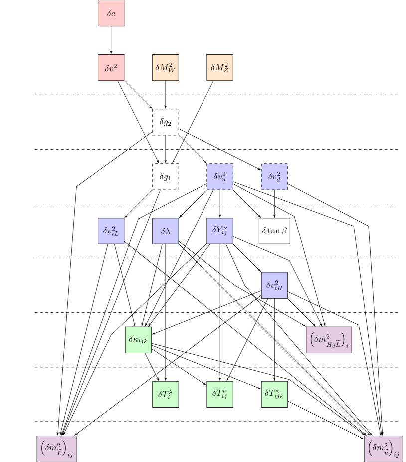
Figure 1: Strategy for extracting the counterterms needed for renormalizing the neutral scalar potential. The arrows indicate the order in which the counterterms were obtained, while the colors stand for the sector that was used to extract the counterterms. Red: Renormalization of electromagnetic coupling. Violet: Renormalization of ${{\cal CP}}$-odd self-energies. Yellow: Renormalization of gauge boson self-energies. Blue: Renormalization of neutral fermion self-energies. Green: Renormalization of ${\cal CP}$-even scalar trilinear couplings. White: Completely fixed by the dependence on other counterterms. The counterterms in the dashed boxes do not belong to the set of independent parameters, but their counterterms were calculated as an intermediate step. The counterterms below one of the horizontal dashed lines could be extracted only after the counterterms above the same horizontal line were determined.

3.3.1 OS conditions

The SM gauge boson masses are renormalized OS requiring

$$\text{Re}\left[{\hat{\Sigma}_{ZZ}}^{T}\left(M_{Z}^{2}\right)\right]=0\qquad\text{and}\qquad\text{Re}\left[{\hat{\Sigma}_{WW}}^{T}\left(M_{W}^{2}\right)\right]=0\;,$$ (3.14)

where $\hat{\Sigma}^{T}$ stands for the transverse part of the renormalized gauge boson self-energy. For their mass counterterms these conditions yield

$$\delta M_{Z}^{2}=\text{Re}\left[{\Sigma}_{ZZ}^{T}\left(M_{Z}^{2}\right)\right]\qquad\text{and}\qquad\delta M_{W}^{2}=\text{Re}\left[{\Sigma}_{WW}^{T}\left(M_{W}^{2}\right)\right]\;.$$ (3.15)

Here the ${\Sigma}^{T}$ (without the hat) denote the transverse part of the unrenormalized gauge boson self-energies.

For the tadpole coefficients $T_{\varphi_{i}}$ the OS conditions read

$$T_{\varphi_{i}}^{(1)}+\delta T_{\varphi_{i}}=0\;,$$ (3.16)

where $T_{\varphi_{i}}^{(1)}$ are the one-loop contributions to the linear terms of the scalar potential, stemming from tadpole diagrams shown in Fig. 2. The tadpole diagrams are calculated in the mass eigenstate basis $h$. The one-loop tadpole contributions in the interaction basis $\varphi$ are then obtained by the rotation

$$T_{\varphi}^{(1)}={U^{H}}^{T}T_{h}^{(1)}\;.$$ (3.17)

Accordingly we find for the one-loop tadpole counterterms

$$\delta T_{\varphi_{i}}=-T_{\varphi_{i}}^{(1)}\;.$$ (3.18)

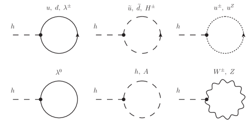
Figure 2: Generic Feynman diagrams for the tadpoles $T_{h_{i}}$.

3.3.2 $\smash{\overline{\mathrm{DR}}}$ conditions

For practical purposes we decided to renormalize all remaining parameters in the $\smash{\overline{\mathrm{DR}}}$ scheme, reflecting the fact that there are no physical observables yet that could be directly related to them. The counterterms of each parameter were obtained by calculating the divergent parts of one-loop corrections to different scalar and fermionic two- and three-point functions. We sketch the determination of the counterterms in the (possible) order in which they can be successively derived (see Fig. 1).

The general strategy for extracting the counterterms of the free parameters is the following. At first one finds a relatively simple tree-level expression, containing the parameter whose counterterm one wants to extract, and, apart from that, exclusively parameters whose countertems are already known. In our case we used bilinear and trilinear couplings in the neutral scalar and fermionic sector for this. Then one calculates the one-loop corrections to the term by evaluating the corresponding Feynman diagrams. As we only need the divergent parts of the loop corrections for $\smash{\overline{\mathrm{DR}}}$ conditions, we are able to calculate the diagrams in the gauge eigenstate basis, where the number of diagrams is drastically reduced. Once the divergent contributions are known, the counterterm to be identified directly follows from the expression of the renormalized Green’s functions.

In this chapter we only state the general formulas for the renormalized two- and three-point Green’s functions. The exact conditions used to extract each countertem is listed in App. B.2. Therein, we also show the resulting analytic expressions for the counterterms renormalized in the $\smash{\overline{\mathrm{DR}}}$ scheme. A more detailed discussion in the case of the $\mu\nu\mathrm{SSM}$ with one generation of right-handed neutrinos can be found in Ref. [99].

Neutral fermion sector

We derived most of the counterterms in the neutral fermion sector. The mass matrix elements of the neutral fermions $\left(m_{\nu}\right)_{ij}$ get one-loop corrections via the neutral fermion self-energies ${\sum}_{\chi_{i}^{0}\chi_{j}^{0}}$, that for Majorana fermions can be decomposed as

$$\Sigma_{\chi_{i}^{0}\chi_{j}^{0}}\left(p^{2}\right)=\not{p}\Sigma_{\chi_{i}^{0}\chi_{j}^{0}}^{F}\left(p^{2}\right)+\Sigma_{\chi_{i}^{0}\chi_{j}^{0}}^{S}\left(p^{2}\right)\;.$$ (3.19)

Defining for the renormalized mass matrix

$$\left(m_{\nu}\right)_{ij}\rightarrow\left(m_{\nu}\right)_{ij}+\delta\left(m_{\nu}\right)_{ij}\;,$$ (3.20)

the renormalized scalar part of the self-energies at zero momentum is given by

$$\hat{\Sigma}_{\chi_{i}^{0}\chi_{j}^{0}}^{S}\left(0\right)=\Sigma_{\chi_{i}^{0}\chi_{j}^{0}}^{S}\left(0\right)-\frac{1}{2}\left(\delta Z_{ki}^{\chi}\left(m_{\nu}\right)_{kj}+\left(m_{\nu}\right)_{ik}\delta Z_{kj}^{\chi}\right)-\delta\left(m_{\nu}\right)_{ij}\;.$$ (3.21)

The field renormalization constants can be obtained in the $\smash{\overline{\mathrm{DR}}}$ scheme by calculating the divergent part of the fermionic piece,

$$\delta Z_{ij}^{\chi}=-\left.\Sigma_{\chi_{i}^{0}\chi_{j}^{0}}^{F}\right|^{\rm div}\;.$$ (3.22)

The divergent parts of the self-energies of the neutral fermions were calculated diagrammatically in the interaction basis, where diagrams with mass insertions have to be included. If $\left(m_{\nu}\right)_{ij}$ containes just a single parameter whose counterterm is unknow, Eq. (3.21) provides a definition for the missing counterterm once the mass counterterm $\delta\left(m_{\nu}\right)_{ij}$ is expressed in terms of the counterterms of the fundamental parameters. Unfortunately, the right-handed vevs $v_{iR}$ always appear in sums over the family index and never isolated. Therefore we calculated loop corrections to the three elements $\left(m_{\nu}\right)_{i,7}=-Y^{\nu}_{ij}v_{jR}/\sqrt{2}$, which provides us with a linear system of three independent equations;

$$Y^{\nu}_{ij}\delta v_{jR}=\sqrt{2}\left.\Sigma_{\nu_{iL}\widetilde{H}^{0}_{u}}^{S}\right|^{\rm div}-\frac{1}{2}\left(\delta Z_{ij}^{\chi}v_{kR}Y^{\nu}_{jk}-\delta Z_{i6}^{\chi}v_{jR}\lambda_{j}+\delta Z_{77}^{\chi}v_{jR}Y^{\nu}_{ij}\right)-v_{jR}\delta Y^{\nu}_{ij}\;,$$ (3.23)

that can be solved analytically for the three counterterms $\delta v_{iR}^{2}=2v_{iR}\;\delta v_{iR}$.

Neutral scalar trilinear couplings

General one-loop scalar three-point functions can be renormalized by wavefunction counterterms and the specific vertex counterterm as

$$\hat{\Gamma}_{\varphi_{i}\varphi_{j}\varphi_{k}}^{(1)}=\Gamma_{\varphi_{i}\varphi_{j}\varphi_{k}}^{(0)}+\Gamma_{\varphi_{i}\varphi_{j}\varphi_{k}}^{(1)}-\frac{1}{2}\biggl{(}\Gamma_{\varphi_{l}\varphi_{j}\varphi_{k}}^{(0)}\delta Z_{li}+\Gamma_{\varphi_{i}\varphi_{l}\varphi_{k}}^{(0)}\delta Z_{lj}+\Gamma_{\varphi_{i}\varphi_{j}\varphi_{l}}^{(0)}\delta Z_{lk}\biggr{)}-\delta\Gamma_{\varphi_{i}\varphi_{j}\varphi_{k}}^{(1)}\;,$$ (3.24)

where $\delta Z_{ij}$ are the scalar field renormailzation constants defined in Eq. (3.10), $\Gamma_{\varphi_{i}\varphi_{j}\varphi_{k}}^{(0)}$ are the tree-level couplings, $\Gamma_{\varphi_{i}\varphi_{j}\varphi_{k}}^{(1)}$ are the one-loop corrections obtained by evaluating the non-irreducible one-loop three-point diagrams, and $\delta\Gamma_{\varphi_{i}\varphi_{j}\varphi_{k}}^{(1)}$ is the coupling counterterm given as a function of the counterterms of the independent parameters. The field renormalization constants are defined as $\smash{\overline{\mathrm{DR}}}$-parameters. We calculate the UV-divergent part of the derivative of the scalar ${{\cal CP}}$-even self-energies in the interaction basis and define

$$\delta Z_{ij}=-\left.\frac{d}{dp^{2}}\Sigma_{\varphi_{i}\varphi_{j}}\right|^{\rm div}\;.$$ (3.25)

As before, if at tree level $\Gamma_{\varphi_{i}\varphi_{j}\varphi_{k}}^{(0)}$ just contains a single parameter whose counterterm is still unknown, the counterterm can be extracted from the divergent part of the one-loop corrections $\Gamma_{\varphi_{i}\varphi_{j}\varphi_{k}}^{(1)}$ demanding that the renormalized quantity is finite. Similarly to the vevs $v_{iR}$, for the parameters $\kappa_{iij}$ it is not possible to find a tree-level expression where each element appears isolated. However, using the renormalized expression in Eq. (3.24) for the vertex

$$\Gamma_{\widetilde{\nu}_{iR}^{\mathcal{R}}\widetilde{\nu}_{kR}^{\mathcal{R}}\widetilde{\nu}_{jL}^{\mathcal{R}}}^{(0)}=\frac{1}{2}v_{d}\lambda_{k}Y^{\nu}_{ji}+\frac{1}{2}v_{d}\lambda_{i}Y^{\nu}_{jk}-\frac{1}{2}v_{lL}Y^{\nu}_{li}Y^{\nu}_{jk}-\frac{1}{2}v_{lL}Y^{\nu}_{lk}Y^{\nu}_{ji}-v_{u}\kappa_{ikl}Y^{\nu}_{jl}\;,$$ (3.26)

we can extract the counterterms for the three subsets $(\delta\kappa_{11j},\delta\kappa_{22j},\delta\kappa_{33j})$ by renormalizing the subset of vertices ($\Gamma_{\widetilde{\nu}_{1R}^{\mathcal{R}}\widetilde{\nu}_{1R}^{\mathcal{R}}\widetilde{\nu}_{jL}^{\mathcal{R}}}$, $\Gamma_{\widetilde{\nu}_{2R}^{\mathcal{R}}\widetilde{\nu}_{2R}^{\mathcal{R}}\widetilde{\nu}_{jL}^{\mathcal{R}}}$, $\Gamma_{\widetilde{\nu}_{3R}^{\mathcal{R}}\widetilde{\nu}_{3R}^{\mathcal{R}}\widetilde{\nu}_{jL}^{\mathcal{R}}}$). Thus, for each subset ($\kappa_{iij}\,;i=1,2,3$) we get a linear system of three ($j=1,2,3$) equations to extract the counterterms $\delta\kappa_{iij}$ from the condition that the renormalized one-loop three-point function is finite.

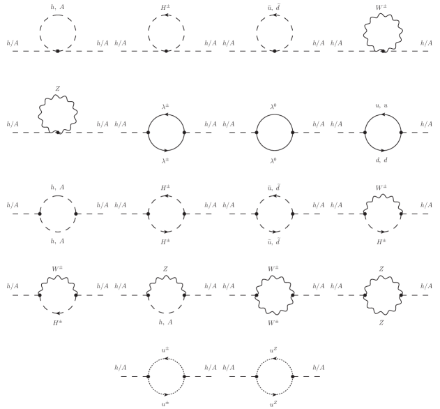
Figure 3: Generic diagrams for the ${{\cal CP}}$-even ($h$) and ${{\cal CP}}$-odd ($A$) scalar self-energies in the mass eigenstate basis.

Neutral scalar masses

The soft scalar masses appear in the bilinear terms of the Higgs potential. They can be renormalized by calculating radiative corrections to scalar self-energies. Since our final aim is to obtain loop corrections for the ${\cal CP}$-even scalars, we used the ${\cal CP}$-odd scalar sector to extract the counterterms of the soft masses to have an independent crosscheck of both neutral scalar sectors.

The general form of the renormalized scalar self-energies at the one-loop level is

$$\hat{\Sigma}_{X_{i}X_{j}}\left(p^{2}\right)= \Sigma_{X_{i}X_{j}}\left(p^{2}\right)+\frac{1}{2}p^{2}\left(\delta Z_{ji}+\delta Z_{ij}\right)$$

$$- \frac{1}{2}\left(\delta Z_{ki}\left(m_{X}^{2}\right)_{kj}+\left(m_{X}^{2}\right)_{ik}\delta Z_{kj}\right)-\delta\left(m_{X}^{2}\right)_{ij}\;,$$ (3.27)

where $X=(\varphi,\sigma)$ represents either the ${{\cal CP}}$-even or the ${{\cal CP}}$-odd scalar fields and we made use of the fact that the field renormalization constants $\delta Z$ and the mass matrix $m_{X}^{2}$ are real. Demanding that the renormalized self-energies $\hat{\Sigma}_{A_{i}A_{j}}$ are finite in the mass eigenstate basis we can define the divergent parts of the mass counterterms via

$$\left.\delta\left(m_{A}^{2}\right)_{ij}\right|^{\rm div}=\left.\Sigma_{A_{i}A_{j}}\left(0\right)\right|^{\rm div}-\frac{1}{2}\left(\left(\delta Z^{A}\right)_{ji}m_{A_{j}}^{2}+m_{A_{i}}^{2}\left(\delta Z^{A}\right)_{ij}\right)\;,$$ (3.28)

where the field counterterms in the mass eigenstate basis were defined in Eq. (3.12), and renormalized as $\smash{\overline{\mathrm{DR}}}$ parameters like the ones for the ${{\cal CP}}$-even scalars (see Eq. (3.25)), and the masses squared $m_{A_{i}}^{2}$ are the eigenvalues of the diagonal ${{\cal CP}}$-odd scalar mass matrix $m_{A}^{2}$. In Fig. 3 we show the diagrams that have to be calculated to obtain the quantum corrections to scalar self-energies at the one-loop level in the mass eigenstate basis.

We calculated all diagrams in the ’t Hooft-Feynman gauge in which the Goldstone bosons $A_{1}$ and $H^{\pm}_{1}$ and the ghost fields $u^{\pm}$ and $u^{Z}$ have the same masses as the corresponding gauge bosons. Calculating the ${{\cal CP}}$-odd self-energies $\Sigma_{A_{i}A_{i}}$ diagrammatically, we obtain the mass counterterms in mass eigenstate basis through the Eq. (3.28). Now inverting the rotation in Eq. (3.9) yields the mass counterterms for the ${{\cal CP}}$-odd self-energies in the interaction basis,

$$\left.\delta m_{\sigma}^{2}\right|^{\rm div}={U^{A}}^{T}\left.\delta m_{A}^{2}\right|^{\rm div}U^{A}\;.$$ (3.29)

Analytically, following the expansion in Eq. (3.8), some of the mass counterterms $\delta m_{\sigma}^{2}$ depend on the counterterms of the soft mass parameters. We use this dependences to extract the counterterms of $(m_{H_{d}\widetilde{L}}^{2})_{i}$ and the counterterms of the non-diagonal elements of $(m_{\widetilde{L}}^{2})_{ij}$ and $(m_{\widetilde{\nu}}^{2})_{ij}$.

4 Loop corrected scalar masses

In the previous section we have defined an OS/$\smash{\overline{\mathrm{DR}}}$ renormalization scheme for the $\mu\nu\mathrm{SSM}$ neutral scalar sector. This can be applied (via the FeynArts model file, in which the counterterms are implemented) to any higher-order correction in the $\mu\nu\mathrm{SSM}$. As a first application, we evaluate the full one-loop corrections to the ${{\cal CP}}$-even scalar sector in the $\mu\nu\mathrm{SSM}$. In the following we emphasize the differences w.r.t the analysis with just one right-handed neutrino from Ref. [99].

4.1 Evaluation at the one-loop level

The one-loop renormalized self-energies in the mass eigenstate basis are given by

$$\hat{\Sigma}_{h_{i}h_{j}}^{(1)}\left(p^{2}\right)=\Sigma_{h_{i}h_{j}}^{(1)}\left(p^{2}\right)+\delta Z^{H}_{ij}\left(p^{2}-\frac{1}{2}\left(m_{h_{i}}^{2}+m_{h_{j}}^{2}\right)\right)-\left(\delta m_{h}^{2}\right)_{ij}\;,$$ (4.1)

with the field renormalization constants $\delta Z^{H}$ and the mass counter terms $\delta m_{h}^{2}$ in the mass eigenstate basis defined by the rotations in Eq. (3.12) and Eq. (3.9), respectively. $\Sigma_{h_{i}h_{j}}$ is the unrenormalized self-energy obtained by calculating the diagrams shown in Fig. 3 with the ${{\cal CP}}$-even states $h$ on the external legs. The self-energies were calculated in the ’t Hooft-Feynman gauge, so that gauge-fixing terms do not yield counterterm contributions in the Higgs sector at the one-loop level. The loop integrals were regularized using dimensional reduction [126, 127] and numerically evaluated for arbitrary real momentum using LoopTools [119]. The contributions from complex values of $p^{2}$ were approximated using a Taylor expansion with respect to the imaginary part of $p^{2}$ up to first order.

In Eq. (4.1) we already made use of the fact that $\delta Z^{H}$ is real and symmetric in our renormalization scheme. The mass counterterms are defined as functions of the counterterms of the free parameters following Eq. (3.8) and Eq. (3.9). They contain finite contributions from the tadpole counterterms and from the counterterm for the gauge boson mass $M_{Z}^{2}$. The matrix $\delta m_{h}^{2}$ is real and symmetric.

The renormalized self-energies enter the inverse propagator matrix

$$\hat{\Gamma}_{h}=\text{i}\left[p^{2}\;\mathbbm{1}-\left(m_{h}^{2}-\hat{\Sigma}_{h}\left(p^{2}\right)\right)\right]\;,\qquad\text{with }\left(\hat{\Sigma}_{h}\right)_{ij}=\hat{\Sigma}_{h_{i}h_{j}}\;.$$ (4.2)

The loop-corrected scalar masses squared are the zeroes of the determinant of the inverse propagator matrix. The determination of corrected masses has to be done numerically when one wants to account for the momentum-dependence of the renormalized self-energies. This is done by an iterative method that has to be carried out for each of the six squared loop-corrected masses.

4.2 Inclusion of higher orders

In Eq. (4.2) we did not include the superscript ⁽¹⁾ in the self-energies. Restricting the numerical evaluation to a pure one-loop calculation would lead to very large theoretical uncertainties. These can be avoided by the inclusion of corrections beyond the one-loop level. Here we follow the approach of Refs. [87, 99] and supplement the $\mu\nu\mathrm{SSM}$ one-loop results by higher-order corrections in the MSSM limit as provided by FeynHiggs (version 2.13.0) [60, 61, 40, 62, 63, 48, 64, 67]. In this way the leading and subleading two-loop corrections are included, as well as a resummation of large logarithmic terms, see the discussion in Sect. 1,

$$\hat{\Sigma}_{h}\left(p^{2}\right)=\hat{\Sigma}_{h}^{(1)}\left(p^{2}\right)+\hat{\Sigma}_{h}^{(2^{\prime})}+\hat{\Sigma}_{h}^{\rm resum}\;.$$ (4.3)

In the partial two-loop contributions $\hat{\Sigma}_{h}^{(2^{\prime})}$ we take over the corrections of ${\cal O}(\alpha_{s}\alpha_{t},\alpha_{s}\alpha_{b},\alpha_{t}^{2},\alpha_{t}\alpha_{b})$, assuming that the MSSM-like corrections approximate numerically well the corresponding $\mu\nu\mathrm{SSM}$ corrections. This assumption is reasonable since the only difference between the squark sector of the $\mu\nu\mathrm{SSM}$ in comparison to the MSSM are numerically suppressed terms proportional to $v_{jL}Y^{\nu}_{jk}v_{kR}$ in the non-diagonal element of the up-type squark mass matrices (see Eq. (2.39)) and proportional to $v_{iL}v_{iL}$ in the diagonal elements of the up- and down-type squark mass matrices (see Eqs. (2.38), (2.40), (2.42) and (2.44)). Furthermore, in Refs. [108, 87] the quality of the MSSM approximation was tested in the NMSSM, showing that the genuine NMSSM contributions are in most cases sub-leading. Our results in Ref. [99] confirm that the same holds true in the $\mu\nu\mathrm{SSM}$ for the SM-like Higgs-boson mass. The same is expected for the contributions stemming from the resummation of large logarithmic terms given by $\hat{\Sigma}_{h}^{\rm resum}$.

5 Numerical analysis

In the following we will present several benchmark points (BPs) that illustrate the phenomenology of the scalar sector of the $\mu\nu\mathrm{SSM}$. We concentrate on scenarios in which a right-handed sneutrino is mixed with the SM-like Higgs boson. By setting $\kappa_{ijk}=\kappa\;\delta_{ij}\delta_{jk}$, as explained in Sect. 2.1, we achieve that only a single right-handed sneutrino substantially mixes with the SM-like Higgs boson. Naturally, the mass scale of the right-handed sneutrinos will then be of the order of the SM-like Higgs boson. However, scenarios in which the decay of the SM-like Higgs boson to two right-handed sneutrinos is kinematically allowed, are experimentally very constrained [109].

In contrast to most of the previous studies of the $\mu\nu\mathrm{SSM}$ with three generations of right-handed neutrinos [24, 25, 27, 28, 109], we will not always make the simplifying assumption that genuine low-energy $\mu\nu\mathrm{SSM}$-parameters have universal values independent of the family index. In Sect. 5.3 we elaborate on the effect of non-universal $\lambda_{i}$ on the SM-like Higgs-boson mass, while keeping $\boldsymbol{\lambda}^{2}=\lambda_{i}\lambda_{i}$ constant. Since we know from Eq. (2.30) that the tree-level mass of the SM-like Higgs boson strongly depends on $\boldsymbol{\lambda}^{2}$, it will be discussed whether the loop corrections increase the dependence on the individual values $\lambda_{i}$.

We consider the following experimental constraints on the scenarios presented:

• We use the public code HiggsBounds v.5.2.0 [130, 131, 132, 133, 134] to determine whether a BP has been excluded by cross section limits from Higgs searches at LEP, LHC or Tevatron. These searches are mostly sensitive to the heavy Higgs and the right-handed sneutrinos, if these are substantially mixed with the SM-like Higgs boson. The production of the left-handed sneutrinos is much smaller at the LHC, and signals from their decay usually demand dedicated searches [30], especially if the left-handed sneutrino is the LSP [31, 29].

• The properties of the SM-like Higgs boson, i.e., its mass and signal rates at LHC and Tevatron, are checked using the public code HiggsSignals v.2.2.1 [135, 136, 137]. Here we assume a theoretical mass uncertainty of $3\,\,\mathrm{GeV}$. HiggsSignals provides us with a $\chi^{2}$-analysis of $n_{\text{obs}}=106$ observables in the 7+8 TeV data package and $n_{\text{obs}}=101$ observables in the 13 TeV data package. In our plots we show the reduced $\chi^{2}_{\mathrm{red}}=\chi^{2}/n_{\mathrm{obs}}$, where a value of $\chi_{\mathrm{red}}^{2}=1$ means that on average the signal rates of the SM-like Higgs boson are at the level of the $\pm 1\sigma$ range of the measurements.

• The properties of the neutrino sector are in agreement with the measurements of the mass-squared differences and the mixing angles obtained from neutrino oscillation experiments. We check that our predictions are within the $\pm 3\sigma$ bands published by the NuFit collaboration [138, 139],

  $$6.80\,\,\mathrm{eV}^{2}\leq\delta m_{12}^{2}/10^{-5}\leq 8.02\,\,\mathrm{eV}^{2}\,,\quad 2.399\,\,\mathrm{eV}^{2}\leq\Delta m_{13}^{2}/10^{-3}\leq 2.593\,\,\mathrm{eV}^{2}\,,$$ (5.1)

  $$0.0198\leq s_{13}^{2}\leq 0.0244\,,\quad 0.272\leq s_{12}^{2}\leq 0.346\,,\quad 0.418\leq s_{23}^{2}\leq 0.613\,,$$ (5.2)

  where we considered the normal mass ordering which is now favored by experiments [140]. A genetic algorithm was used to find parameter points that minimize the sum of squared deviations between theoretical prediction and experimental values specified above [141]. Even though the $\mu\nu\mathrm{SSM}$ allows for flavor-violating decays of leptons, the existing experimental bounds (for instance on $\mu\rightarrow e\gamma$) are automatically fulfilled when the constrains on neutrino masses are taken into account [26].

For the necessary input of HiggsBounds and HiggsSignals we compute the decays of the scalars at leading order, but with the loop-corrected mixing matrix elements inserted in the expressions of the scalar couplings. In the limit of vanishing external momentum, which we used in the determination of the mixing matrix elements for the couplings, this method corresponds to include the finite wave-function renormalization factors ($Z$-factors) for each external scalar [142, 63]. For loop-induced decays and off-shell decays to vector bosons we implemented analytic results from the MSSM well known in the literature [143, 144, 145, 146, 147], and scaled the expressions with effective couplings defined by the mixing matrix elements and $\tan\beta$ to obtain the result for the scalars in the $\mu\nu\mathrm{SSM}$. For the coupling to $b$ quarks we included the running bottom mass and for the decay to gluons the running of $\alpha_{s}$ from $M_{Z}$ to the mass of the decaying scalar, and finally add leading higher-order QCD corrections [148, 145].

As described in Sect. 2.5 we use the left-handed vevs $v_{iL}$, the soft gaugino masses $M_{1}$ and $M_{2}$, and the neutrino Yukawa couplings $Y^{\nu}_{ij}$ to fit the neutrino masses and mixings accurately, making use of the fact that they can be modified without spoiling the properties of the SM-like Higgs boson. Besides for the scenario presented in Sect. 5.4, it will be sufficient to just consider diagonal non-zero elements of $Y^{\nu}_{ij}$. Because we concentrate here on the scalar sector of the $\mu\nu\mathrm{SSM}$, and since the fitting has to be done numerically, we do the fitting in our scans just in one particular point for each analysis. By varying a parameter, the prediction for the neutrino properties can be outside the experimentally allowed range in some points. We indicate in our plots when this is the case. Since the neutral fermion mass matrix is of dimension 10, with large hierarchies between the neutrino sector and the remaining part, including one-loop corrections is time-consuming and numerically very challenging. Therefore we stick to a tree-level analysis for the neutrinos. However, we checked for several points that the one-loop corrections are sub-leading and can in principle be compensated by a slight change of the parameters.

5.1 Scan over $\lambda$

$\tan\beta$	$\lambda$	$\kappa$	$v_{1,3R}$	$v_{2R}$	$A^{\lambda}$	$A^{\kappa}$	$A^{\nu}$
$5$	$[0.13,0.18]$	$0.5$	$1000$	$765$	$1000$	$-1000$	$-1000$
$A^{u}_{3}$	$A^{u}_{1,2}$	$A^{d,e}$	$m_{\widetilde{Q},\widetilde{u},\widetilde{d}}$	$m_{\widetilde{e}}$	$M_{3}$
$-2000$	$-1500$	$-1500$	$1500$	$200$	$2700$
$v_{1L}/10^{-4}$	$v_{2L}/10^{-4}$	$v_{3L}/10^{-4}$	$Y^{\nu}_{11}/10^{-7}$	$Y^{\nu}_{22}/10^{-7}$	$Y^{\nu}_{33}/10^{-7}$	$M_{1}$	$M_{2}$
$1.390$	$6.215$	$4.912$	$4.181$	$1.756$	$6.306$	$1228$	$2814$

Table 2: Low-energy values for the parameters, as defined in the text, of the scan over $\lambda$. Dimensionful parameters are given in GeV. The parameters in the last row are fitted to neutrino oscillation data.

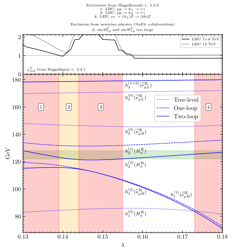
Figure 4: ${{\cal CP}}$-even scalar spectrum in the scan over $\lambda$ at tree level, one-loop level and partial two-loop level. We show in the brackets the dominant composition of the tree-level, one-loop and two-loop mass eigenstates $h^{(0)}$, $h^{(1)}$ and $h^{(2)}$, in the experimentally allowed region of the plot. The desired SM-like Higgs-boson mass is indicated with the horizontal green band, assuming a theory uncertainty of $3\,\,\mathrm{GeV}$. The red regions are excluded by direct searches for additional scalars. In the yellow region the prediction for the mixing angles of the neutrinos lies outside of the 3$\sigma$ band of the experimental measurement. On top we show $\chi_{\mathrm{red}}^{2}$ for various Higgs-boson signal strength measurements at LHC.

The first scenario we are presenting is one with a light right-handed $\mu$-sneutrino that mixes substantially with the SM-like Higgs boson. We show the chosen parameters in Tab. 2. To simplify the notation we define $\lambda=\lambda_{i}$, $A^{\lambda}=A^{\lambda}_{i}$, $A^{\nu}=A^{\nu}_{ii}$, $\kappa=\kappa_{iii}$ and $A^{\kappa}=A^{\kappa}_{iii}$ and vanishing otherwise. The soft parameters are given in terms of $A^{d}=A^{d}_{i}$, $A^{e}=A^{e}_{ii}$, $m_{\widetilde{Q}}=m_{\widetilde{Q}_{i}}$, $m_{\widetilde{u}}=m_{\widetilde{u}_{i}}$, $m_{\widetilde{d}}=m_{\widetilde{d}_{i}}$, and $m_{\widetilde{e}}=m_{\widetilde{e}_{ii}}$ and vanishing otherwise. We vary over the universal parameter $\lambda$, while keeping the remaining parameters fixed. For the right-handed $e$- and $\tau$-sneutrino vevs we chose $v_{1,3R}=1\,\,\mathrm{TeV}$, but set a smaller value of $v_{2R}=765\,\,\mathrm{GeV}$ for the $\mu$-sneutrino vev to decrease the mass of the ${{\cal CP}}$-even $\mu$-sneutrino to the range around the SM-like Higgs-boson mass. The choice to pick $\widetilde{\nu}_{\mu R}$ as the light right-handed sneutrino is of no relevance. The large value of $\kappa=0.5$ assures that the other two right-handed sneutrinos will have masses between $300$ and $400\,\,\mathrm{GeV}$, well above $125\,\,\mathrm{GeV}$. Because the SM-like Higgs boson mass will get additional contributions from the mixing with $\widetilde{\nu}_{\mu R}^{\mathcal{R}}$, $\tan\beta$ can be chosen rather low.

As mentioned in the previous subsection, we fit the properties of the neutrinos in just one particular point of the parameter scan. In this scenario, this was done for $\lambda=0.168$, leading to the values of $v_{iL}$, $Y^{\nu}_{ii}$, $M_{1}$ and $M_{2}$ shown in Tab. 2. We emphasize that this effectively leaves just the trilinear parameters $A^{\nu}_{ii}$ to adjust the masses of the left-handed sneutrinos. For the prediction of the masses of the right-handed sneutrinos and the SM-like Higgs boson, the fitted parameters only play a minor role.

In Fig. 4 we show the resulting spectrum of the light ${{\cal CP}}$-even scalars. The remaining ${{\cal CP}}$-even scalars not shown in the plot have masses above $300\,\,\mathrm{GeV}$ and do not play a role in the following discussion. The dotted lines represent the tree-level masses, the dashed lines the masses including the full one-loop corrections, and the solid lines the one-loop + partial two-loop + resummed (referred to as two-loop in the following) corrected masses, as explained in Sect. 4.2. We mark four regions in the plot which are excluded either by HiggsBounds (red), or by not being in agreement with the neutrino oscillation data (yellow). We stress that region 2 is just excluded for the precise choice of parameters shown in Tab. 2. A new fit of the neutrino properties for each value of $\lambda$ could easily accommodate predictions for the properties of the neutrinos in agreement with experiments. However, since this would exclusively affect the phenomenology of the heavier left-handed sneutrinos in the scalar sector, we do not apply the fit for each value of $\lambda$.

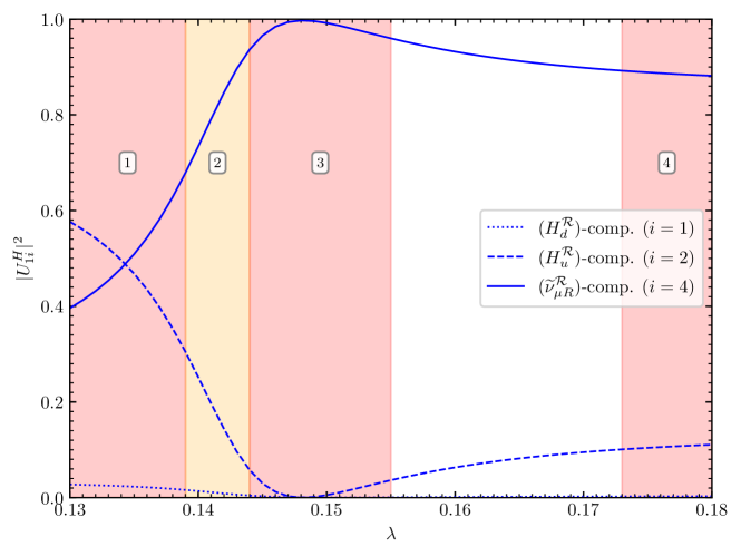
Figure 5: Doublet components ($H_{d}^{\mathcal{R}}$, $H_{u}^{\mathcal{R}}$) and the right-handed $\mu$-sneutrino component ($\widetilde{\nu}_{\mu R}^{\mathcal{R}}$) of the lightest ${{\cal CP}}$-even mass eigenstate $h_{1}$, which are defined by $|U^{H}_{1i}|^{2}$ with $i=1,2$ and $i=4$ respectively.

This spectrum is characterized by the interplay between the light $\widetilde{\nu}_{\mu R}^{\mathcal{R}}$ and the SM-like Higgs boson. For small $\lambda$ the two lightest loop-corrected mass eigenstates $h_{1}$ and $h_{2}$ have roughly an equal amount of $H_{u}^{\mathcal{R}}$- and $\widetilde{\nu}_{\nu R}^{\mathcal{R}}$-admixture (see also Fig. 5). Consequently, region 1 is excluded by direct searches at the LHC, because the diphoton resonance search for a SM-like higgs boson excludes $h_{1}$ via its decay to photons [149]. At $\lambda\sim 0.14$ the point is reached where the mass of $h_{1}$ drops well below $125\,\,\mathrm{GeV}$. Thus, beyond that point $h_{1}$ can be identified with $\widetilde{\nu}_{\mu R}^{\mathcal{R}}$, as the doublet-component of $h_{1}$ shrinks to values of roughly $\sim 10\%$. $h_{2}$, on the other hand, sheds its sneutrino admixture, so that it can be identified as the SM-like Higgs boson, and the large quantum corrections from the top/stop sector dominantly contribute to the mass of $h_{2}$. This yields an increase of the SM-like Higgs boson mass of several GeV, so that beyond region 3 it agrees with the experimental value, assuming a theoretical uncertainty of $3\,\,\mathrm{GeV}$.

An interesting observation is that in the allowed region of $\lambda$ the large one-loop corrections change the order of $\widetilde{\nu}_{\mu R}^{\mathcal{R}}$ and the SM-like Higgs boson. While the large shift of the SM-like Higgs-boson mass from $\sim 83\,\,\mathrm{GeV}$ at tree level to $\sim 125\,\,\mathrm{GeV}$ at two-loop level are familiar from the MSSM, the large one-loop corrections to $\widetilde{\nu}_{\mu R}^{\mathcal{R}}$, with a tree-level mass of $\sim 147\,\,\mathrm{GeV}$ and a two-loop mass below $100\,\,\mathrm{GeV}$, emphasize the importance of accurately taking into account the full parameter space of the $\mu\nu\mathrm{SSM}$.

Figure 6: Effective couplings of the two light ${{\cal CP}}$-even scalar mass eigenstates $h_{1}^{(2)}$ (red) and $h_{2}^{(2)}$ (blue) to up-type quarks (solid) and down-type quarks (dashed), normalized to the SM prediction.

In the allowed region the doublet component of $\widetilde{\nu}_{\mu R}^{\mathcal{R}}$ reaches values of approximately $10\%$, which can be seen in Fig. 5, where we plot the down- and up-type doublet component $H_{d}^{\mathcal{R}}$ and $H_{u}^{\mathcal{R}}$, and the $\widetilde{\nu}_{\mu R}^{\mathcal{R}}$-component of the lightest ${{\cal CP}}$-even scalar mass eigenstates $h_{1}^{(2)}$. Naturally, this mixing will also affect the SM-like Higgs-boson properties. In this way, scenarios like the one shown here will be tested by experiments in two different and complementary ways, both caused by the mixing of $\widetilde{\nu}_{\mu R}^{\mathcal{R}}$ and the SM-like Higgs boson: Firstly, direct searches for additional Higgs bosons can be applied to $\widetilde{\nu}_{\mu R}^{\mathcal{R}}$, because it is directly coupled to SM particles. Secondly, precise measurements of the SM-like Higgs-boson couplings can detect (or exclude) possible variations from SM predictions. To illustrate the possible modifications, we show in Fig. 6 the effective coupling of the two light ${{\cal CP}}$-even scalar mass eigenstates to up- and down-type quarks normalized to the SM-prediction which in good approximation can be expressed via the loop-corrected mixing matrix elements $U^{H(2)}_{ij}$ and $\beta$;

$$c_{h_{i}dd}=\frac{U_{i1}^{H(2)}}{\cos\beta}\;,\qquad c_{h_{i}uu}=\frac{U_{i2}^{H(2)}}{\sin\beta}\;.$$ (5.3)

In the experimentally allowed region the effective coupling of the SM-like Higgs boson to up-type quarks shows deviations of roughly $10\%$. This is of the order of precision expected by measurements of the SM Higgs boson couplings at the High-Luminosity LHC [150], and (depending on the center-of-mass energy deployed) an order of magnitude larger than the uncertainty expected for these kind of measurements at a possible future $e^{+}e^{-}$ collider like the ILC  [151, 152, 153]. Comparing to Fig. 4 we can see that the region where the effective couplings are closest to one, meaning equal to the SM prediction, does not coincide with the region where the $\chi_{\mathrm{red}}^{2}$ from HiggsSignals is minimized. This is because the mass of the SM-like Higgs boson is slightly too small in this range of $\lambda$, so even including a theoretical uncertainty of $3\,\,\mathrm{GeV}$ some signal strength measurements implemented in HiggsSignals are not accounted for by $h_{2}$ and $\chi_{\mathrm{red}}^{2}$ becomes worse.

5.2 Scan over $v_{R}$

In Sect. 5.1 we showed that light right-handed sneutrinos with masses in the vicinity of the SM-like Higgs boson are theoretically possible and can induce measurable modifications of the SM-like Higgs-boson properties. Using data of direct searches and measurements of the couplings of the SM-like Higgs boson, the parameter space of these scenarios can be constrained effectively. In this section we present a scenario that is not excluded by current searches in which all three of the ${{\cal CP}}$-even right-handed sneutrinos will have masses below $125\,\,\mathrm{GeV}$. We chose the parameters appearing in the mass terms of the $\widetilde{\nu}_{iR}^{\mathcal{R}}$ to be universal, i.e., $\lambda\mathrel{\mathop{\mathchar 58\relax}}=\lambda_{i}$, $v_{R}\mathrel{\mathop{\mathchar 58\relax}}=v_{iR}$, $\kappa\mathrel{\mathop{\mathchar 58\relax}}=\kappa_{iii}$, $A^{\lambda}\mathrel{\mathop{\mathchar 58\relax}}=A^{\lambda}_{i}$, $A^{\nu}\mathrel{\mathop{\mathchar 58\relax}}=A^{\nu}_{ii}$ and $A^{\kappa}\mathrel{\mathop{\mathchar 58\relax}}=A^{\kappa}_{iii}$. As explained at the beginning of Sect. 5, the universality of $\kappa$ assures that only one of the $\widetilde{\nu}_{iR}^{\mathcal{R}}$ mixes substantially with the SM-like Higgs boson, while the other two are practically decoupled. This makes it easier to control the total admixture of the doublet components of the $\widetilde{\nu}_{iR}^{\mathcal{R}}$.

$\tan\beta$	$\lambda$	$\kappa$	$v_{R}$	$A^{\lambda}$	$A^{\kappa}$	$A^{\nu}$
$9.0$	$0.08$	$0.3$	$[1210,1270]$	$1000$	$-1000$	$-1000$
$A^{u,d,e}$	$m_{\widetilde{Q},\widetilde{u},\widetilde{d}}$	$m_{\widetilde{e}}$	$M_{3}$
$-1000$	$1000$	$200$	$2700$
$v_{1L}/10^{-5}$	$v_{2L}/10^{-5}$	$v_{3L}/10^{-4}$	$Y^{\nu}_{11}/10^{-7}$	$Y^{\nu}_{22}/10^{-7}$	$Y^{\nu}_{33}/10^{-8}$	$M_{1}$	$M_{2}$
$1.466$	$8.520$	$1.855$	$2.963$	$5.337$	$5.902$	$175.6$	$188.0$

Table 3: The same as in Tab. 2 for the scan over $v_{R}=v_{iR}$.

The complete set of free parameters is shown in Tab. 3. In this scenario we scan over $v_{R}$, because they appear linearly in the Majorana-like mass terms of the $\widetilde{\nu}_{iR}^{\mathcal{R}}$, so it is a convenient parameter to control their masses. Compared to the scan over $\lambda$ in Sect. 5.1 the overall behavior of the SM-like Higgs boson is aligned more to the SM predictions by decreasing $\lambda$. Consequently, because at tree level the additional contribution proportional to $\boldsymbol{\lambda}^{2}$ is smaller, $\tan\beta$ is larger to increase the quantum corrections to the SM-like Higgs-boson mass. We also decrease $\kappa$ to make the masses of the $\widetilde{\nu}_{iR}^{\mathcal{R}}$ smaller. As before, the parameters in the last row of Tab. 3 were fitted to accurately predict the left-handed neutrino masses and mixings. The fit was done in the point $v_{R}=1226\,\,\mathrm{GeV}$, but in this case the neutrino data is described accurately over the whole range of $v_{R}$ at tree level.

In Fig. 7 we show the resulting light ${{\cal CP}}$-even scalar spectrum. In the experimentally allowed region ($1213\,\,\mathrm{GeV}\leq v_{R}\leq 1235\,\,\mathrm{GeV}$) the lightest mass eigenstates are two almost degenerate right-handed sneutrinos. The third right-handed sneutrino is roughly $20\,\,\mathrm{GeV}$ heavier, and it acquires substantial mixing with the SM-like Higgs boson. Naturally, the $\widetilde{\nu}_{iR}^{\mathcal{R}}$ increase their masses when $v_{R}$ becomes larger, but also the SM-like Higgs boson mass increases, because the mixing with the $\widetilde{\nu}_{3R}^{\mathcal{R}}$ gives additional contributions.

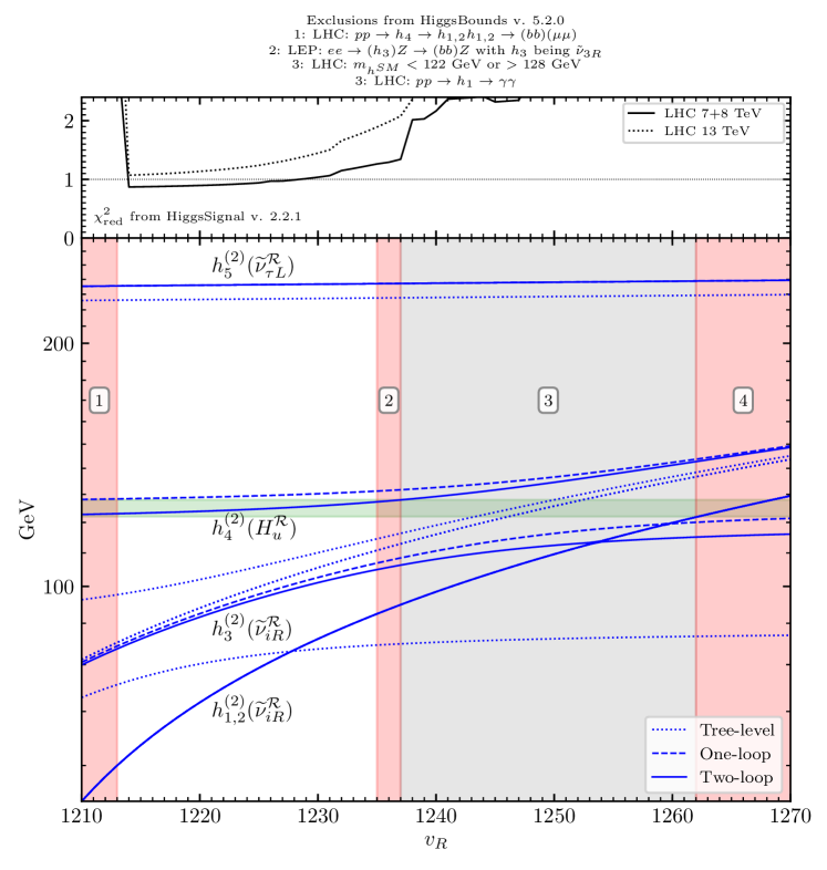
Figure 7: Light ${{\cal CP}}$-even scalar spectrum in the scan over $v_{R}$. Shown are the masses at tree level (dotted), at the one-loop level (dashed) and at the partial two-loop level (solid). We show in the brackets the dominant composition of the loop-corrected mass eigenstates $h^{(2)}$ in the experimentally allowed region of $v_{R}$. The desired SM-like Higgs-boson mass is indicated with the horizontal green band, assuming a theory uncertainty of $3\,\,\mathrm{GeV}$. The red regions are excluded by direct searches for additional scalars. In the gray region the SM-like Higgs-boson mass is not predicted accurately. On top we show $\chi_{\rm red}^{2}$ for various Higgs-boson signal strength measurements at LHC.

The scenario is excluded experimentally for very small values of $v_{R}$, because the two lightest mass eigenstates $h_{1,2}$ become lighter than half the mass of the SM-like Higgs boson $h_{4}$, so the decays of $h_{4}$ into $h_{1,2}$ opens up. Experimental searches for the decay of the SM-like Higgs boson into two lighter scalars that subsequently decay into two $b$-jets and a pair of $\mu$-leptons [154] exclude region 1 in Fig. 7. These additional decay channels of the SM-like Higgs boson are also the reason why the $\chi^{2}_{\mathrm{red}}$ rapidly increases in region 1, because it suppresses ordinary SM-like decays of $h_{4}$.

When $v_{R}$ increases above $1235\,\,\mathrm{GeV}$ further constrains from direct searches for additional Higgs bosons and measurement of the properties of the SM-like Higgs boson become relevant. $\chi_{\mathrm{red}}^{2}$ quickly increases above 2 at $v_{R}\sim 1237\,\,\mathrm{GeV}$. Already at $v_{R}\sim 1235\,\,\mathrm{GeV}$ the scenario is excluded by LEP searches [155]. Note, that in the red region 2 the mixing of $\widetilde{\nu}_{3R}^{\mathcal{R}}$ with the SM-like Higgs boson enlarges, while $\widetilde{\nu}_{3R}^{\mathcal{R}}$ is kinematically still in reach of being produced at LEP via the Higgsstrahlung-process. Consequently, the channel $ee\rightarrow(h_{3})Z\rightarrow(b\bar{b})Z$, where $h_{3}$ is identified with $\widetilde{\nu}_{3R}^{\mathcal{R}}$, excludes this interval. Interestingly, in the experimentally allowed region, where the mass of $\widetilde{\nu}_{3R}^{\mathcal{R}}$ is even smaller, LEP data cannot rule out this scenario. The reasons for this is not only the smaller mixing of $\widetilde{\nu}_{3R}^{\mathcal{R}}$ with the SM-like Higgs boson, but also that in the mass range below $100\,\,\mathrm{GeV}$ LEP saw a slight excess over the SM background (see also Sect. 5.4) [155].

Beyond region 2 the current scenario is experimentally excluded by the measurement of the SM-like Higgs-boson mass in the gray region 3 and by the LHC cross section measurement of the process $pp\rightarrow h_{1}\rightarrow\gamma\gamma$ in region 4 [156]. This is because in region 3 the cross-over point is reached, in which the masses of the $\widetilde{\nu}_{iR}^{\mathcal{R}}$ become larger than the SM-like Higgs-boson mass. Through the interference effects the SM-like Higgs-boson mass is pushed to lower values beyond that point. In region 4 the mass eigenstate corresponding to the SM-like Higgs boson is the lightest one at just about $118\,\,\mathrm{GeV}$. Even though there are two scalars in the mass range of the experimentally measured Higgs-boson mass, there is no contribution to any signal-strength measurement at the LHC, reflected by the fact that the $\chi_{\rm red}^{2}$ is huge in region 4. The reason is that these states correspond to the practically singlet like right-handed neutrino states. The third right-handed sneutrino carrying the doublet admixture taken from the SM-like Higgs boson has a mass of over $140\,\,\mathrm{GeV}$. Hence, it also does not contribute to signal-strength measurements of the SM-like Higgs boson.

On a side note we briefly discuss the remaining light scalar $h_{5}$ in Fig. 7, which is the left-handed $\tau$-sneutrino at roughly $235$–$240\,\,\mathrm{GeV}$. The fit to the neutrino oscillation data generated a hierarchy between the vevs of the left-handed sneutrinos, with $v_{3L}$ being the largest. As a result, since dominant tree-level contributions to the $\widetilde{\nu}_{iL}^{\mathcal{R}}$-masses scale with inverse of $v_{iL}$ (see Eq. (2.31)), the $\widetilde{\nu}_{\tau L}^{\mathcal{R}}$ is the lightest ${{\cal CP}}$-even left-handed sneutrino. It is rather invisible to usual searches for additional Higgs bosons at colliders, but a dedicated analysis of LHC data was proposed to search for light left-handed sneutrinos in the framework of the $\mu\nu\mathrm{SSM}$ [30]. However, the analysis in Ref. [30] concentrated on $\tau$-sneutrinos as the LSP, whereas here there are even lighter SUSY particles in the spectrum. For a detailed discussion of distinct signatures at the LHC related to left-handed sneutrinos within the $\mu\nu\mathrm{SSM}$ we refer to the literature [29, 30, 31].

5.3 Scan over $\lambda_{i}$ while $\boldsymbol{\lambda}^{2}=\lambda_{i}\lambda_{i}=\text{const.}$

As already explained at the beginning of this section, there is no theoretical reason to choose the $\mu\nu\mathrm{SSM}$-like parameters universal w.r.t. the family index. While the tree-level upper bound on the lightest ${{\cal CP}}$-even scalar mass approximately depends on the term $\boldsymbol{\lambda}^{2}=\lambda_{i}\lambda_{i}$, and not on the individual $\lambda_{i}$, this is not the case for the SM-like Higgs-boson mass, as soon as mixing-effects induced by the right-handed sneutrinos are considered. This effects can enter at tree level, or via radiative corrections proportional to $\lambda_{i}$. These radiative corrections depend on the masses and the mixing of each of the right-handed sneutrino. Since it is not the case that all three $\widetilde{\nu}_{iR}$ are degenerate, the radiative corrections are expected to depend strongly on the individual values of $\lambda_{i}$. Also, when $\boldsymbol{\lambda}^{2}$ is fixed, the $\mu$-term which is dynamically generated after EWSB and linearly dependent on $\lambda_{i}$ cannot be constant when the $\lambda_{i}$ are varied. This can be another source of corrections to the SM-like Higgs-boson mass that explicitly depend on the individual values of the $\lambda_{i}$.

However, the loop corrections proportional to $\lambda_{i}$ are an order of magnitude smaller than the ones stemming from the (s)top-sector, partially because quantum contributions to the SM-like Higgs-boson mass at the one-loop level proportional to $\lambda_{i}$ depend on the singlet-admixture of the SM-like Higgs boson which, in turn, cannot be too large to not spoil the measured signal strengths at the LHC. Nevertheless, we will give here a rough idea of how large the remnant effect of non-universal $\lambda_{i}$ on the SM-like Higgs-boson mass can be while $\boldsymbol{\lambda}^{2}$ is kept constant. We performed a parameter scan over all possible values of the $\lambda_{i}$ in a scenario in which $\widetilde{\nu}_{\mu R}^{\mathcal{R}}$ has a mass between $92$ and $115\,\,\mathrm{GeV}$ and mixes substantially with the SM-like Higgs boson. The free parameters were set to the values shown in Tab. 4.

$\tan\beta$	$\boldsymbol{\lambda}^{2}$	$\kappa$	$v_{1,3R}$	$v_{2R}$	$A^{\lambda}$	$A^{\kappa}$	$A^{\nu}$
$5$	$3\cdot 0.168^{2}$	$0.5$	$1000$	$765$	$1000$	$-1000$	$-1000$
$A^{u}_{3}$	$A^{u}_{1,2}$	$A^{(d,e)}$	$m_{\widetilde{Q},\widetilde{u},\widetilde{d}}$	$m_{\widetilde{e}}$	$M_{3}$
$-2000$	$-1500$	$-1500$	$1500$	$200$	$2700$
$v_{1L}/10^{-4}$	$v_{2L}/10^{-4}$	$v_{3L}/10^{-4}$	$Y^{\nu}_{11}/10^{-7}$	$Y^{\nu}_{22}/10^{-7}$	$Y^{\nu}_{33}/10^{-7}$	$M_{1}$	$M_{2}$
$1.497$	$6.179$	$4.946$	$4.388$	$1.759$	$6.258$	$1228$	$2814$

Table 4: The same as in Tab. 2 for the scan over $\lambda_{i}$ while $\boldsymbol{\lambda}^{2}=\text{const}$.

On can see that the scenario is very similar to the one in Sect. 5.1. When the $\lambda_{i}$ are chosen uniformly we recover the BP at $\lambda=0.168$ in Fig. 4 which lies in the middle of the experimentally allowed parameter region. In Fig. 8 we illustrate the dependence of the SM-like Higgs-boson mass on the individual values of $\lambda_{i}$. We show triangle plots [157] with the values of $\lambda_{i}^{2}$ on the axes and with their sum $\boldsymbol{\lambda}^{2}=\text{const}$. The colors of the points indicate the mass of the SM-like Higgs boson at tree level (top left), at one-loop level (top right), the difference of the SM-like Higgs-boson mass at tree level and one-loop level (bottom left), and the one-loop mass of the right-handed $\mu$-sneutrino (bottom right) which is the lightest ${{\cal CP}}$-even scalar in this scenario. We do not show the two-loop mass of the SM-like Higgs boson, because the two-loop corrections supplemented from FeynHiggs are purely MSSM-like corrections independent of $\lambda_{i}$, thus not playing a role in the following discussion. However, the parameters are chosen such that the corrections beyond the one-loop level shift the SM-like Higgs-boson mass into the vicinity of $\sim 125\,\,\mathrm{GeV}$ (see below). In the upper right plot one sees that the one-loop mass of the SM-like Higgs boson is the largest in the central point in which all $\lambda_{i}$ are equal. The tree-level mass, on the other hand, shows the opposite behavior and is the largest in the corners of the upper left plot in which one of the $\lambda_{i}$ is practically zero. The one-loop mass varies in the experimentally allowed region by more than $1\,\,\mathrm{GeV}$. This demonstrates that for an accurate prediction of the SM-like Higgs-boson mass it is crucial to include the independent contributions of all three $\lambda_{i}$ to the radiative corrections, when mixing effects between the right-handed sneutrinos and the SM-like Higgs boson are sizable.

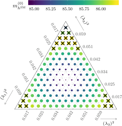
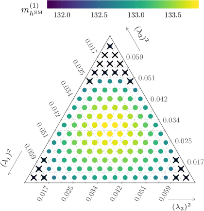
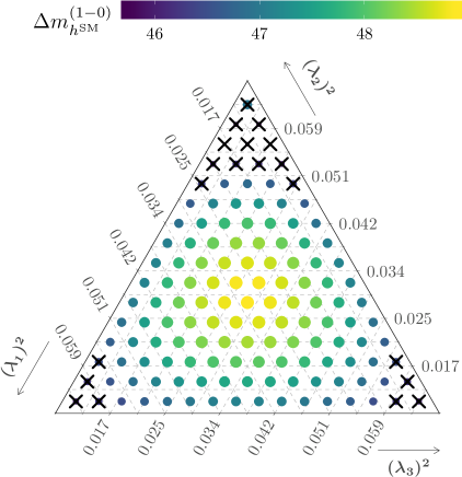
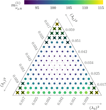
Figure 8: SM-like Higgs-boson mass at tree level $m_{h^{\mathrm{SM}}}^{(0)}=m_{h_{1}^{(0)}}$ (top left), and at one-loop level $m_{h^{\mathrm{SM}}}^{(1)}=m_{h_{2}^{(1)}}$ (top right), and their difference $\Delta m_{h^{\mathrm{SM}}}^{(1-0)}=m_{h^{\mathrm{SM}}}^{(1)}-m_{h^{\mathrm{SM}}}^{(0)}$ (bottom left), and the one-loop mass of $\widetilde{\nu}_{\mu R}$ (bottom right) for fixed $\boldsymbol{\lambda}^{2}$ but varying $\lambda_{i}$, indicated by the colors (and sizes for better visibility). Crossed points are excluded by either HiggsBounds, HiggsSignals with $\chi^{2}_{\rm red}\geq 150/101=1.485$ for the $13\,\,\mathrm{TeV}$ data set, or because the SM-like Higgs boson mass including the two-loop corrections is smaller than 123 GeV or larger than 127 GeV.

Note that the variation of the one-loop mass would be even larger if we neglect the experimental constrains. In this scenario, the main exclusion limit is the requirement to have the SM-like Higgs-boson mass above $123\,\,\mathrm{GeV}$ at two-loop. In the corners of the plots, the mass of $\widetilde{\nu}_{\mu R}^{\mathcal{R}}$, shown in the lower right plot, increases to values very close to the SM-like Higgs-boson mass. This increases the mixing between both scalars which, in turn, reduces the radiative one-loop corrections to the SM-like Higgs boson. Practically speaking, parts of the loop-corrections “are lost” to $\widetilde{\nu}_{\mu R}^{\mathcal{R}}$. This is why the difference between the tree-level and the one-loop mass of the SM-like Higgs boson, shown in the lower left plot of Fig. 8, is the smallest when the mass of $\widetilde{\nu}_{\mu R}^{\mathcal{R}}$ is the largest.

We also emphasize that the variation of the difference between tree-level and one-loop mass, as a measure for the size of genuine one-loop corrections, is more than twice as large as the variation of the one-loop mass of the SM-like Higgs boson. One can see a compensation of lower tree-level mass, but larger loop corrections in the center of the plots, leading to a more stable one-loop mass of the SM-like Higgs boson. This is due to the fact that the loop-corrected mass eigenstate of the SM-like Higgs boson is the physical state, whose properties are constrained by the experimental measurements. Therefore, the singlet-admixture cannot be very large at loop-level, and the parameter dependence of the SM-like Higgs-boson mass induced by this admixture necessarily cannot be too large. The tree-level state, on the other hand, is not physical and can have larger mixing with $\widetilde{\nu}_{\mu R}^{\mathcal{R}}$, leading to a stronger dependence on parameters related to the sneutrinos, like $\lambda_{i}$ in this case. Thus, even though the overall dependence of the SM-like Higgs-boson mass on parameters beyond the MSSM can be very large at tree level, the dependence will be diminished at loop-level in the parameter space that fulfills experimental constraints on the SM-like Higgs-boson properties.

5.4 CMS and LEP excess at $\sim 96\,\,\mathrm{GeV}$

Searches for the SM Higgs boson at LEP can nowadays be used to constrain the parameter space of models with additional scalar particles with masses below the SM-like Higgs-boson mass. Interestingly, an excess over the SM background was observed at a mass of $95$-$98\,\,\mathrm{GeV}$ in the Higgsstrahlung production channel with an associated decay of the Higgs boson to a pair of $b$-quarks [155]. Assuming that this excess can be explained by an additional Higgs boson, the signal strength, i.e, the cross section times branching ratio to $b$-quarks normalized to the SM prediction for a SM-like Higgs boson at the same mass, was extracted in Ref. [158] to be

$$\mu_{\mathrm{LEP}}=0.117\pm 0.057\;.$$ (5.4)

At about the same mass, CMS observed an excess over the SM background in the $pp$ production with associated decay to diphotons in the $8\,\,\mathrm{TeV}$ and the $13\,\,\mathrm{TeV}$ data [159, 160]. For the CMS excess, the signal strength was reported in Refs. [161, 160] to be

$$\mu_{\mathrm{CMS}}=0.6\pm 0.2\;.$$ (5.5)

In a previous publication, we showed that it is possible to accommodate both excesses simultaneously at the $1\sigma$ level in the $\mu\nu\mathrm{SSM}$ with just one right-handed neutrino [99]. We described how a right-handed sneutrino at $\sim 96\,\,\mathrm{GeV}$ can acquire substantial couplings to SM particles via its mixing with the SM-like Higgs boson. However, we did not include an accurate prediction of the properties of the neutrinos in our analysis in the $\mu\nu\mathrm{SSM}$ with one generation of right-handed neutrinos, because in that case at least one neutrino mass has to be generated via quantum corrections. On the contrary, in the $\mu\nu\mathrm{SSM}$ with three generations of right-handed neutrinos, we can describe the mass differences and mixings of the neutrinos at tree level, which is of course much more feasible.

$\tan\beta$	$\lambda_{1,2}$	$\lambda_{3}$	$\kappa_{111,222}$	$\kappa_{333}$	$v_{1,2R}$	$v_{3R}$	$A^{\lambda}_{1,2}$	$A^{\lambda}_{3}$
$1.945$	$0.01$	$[0.538,0.542]$	$0.3$	$0.05$	$1200$	$[884,888]$	$1000$	$[806,814]$
$A^{\nu}_{ii}$	$A^{\kappa}_{111,222}$	$A^{\kappa}_{333}$	$A^{u}_{3}$	$A^{u}_{1,2}$	$A^{d,e}$	$m_{\widetilde{Q},\widetilde{u},\widetilde{d},\widetilde{e}}$	$M_{1}$	$M_{2}$	$M_{3}$
$-1000$	$-300$	$[-124,-100]$	$-650$	$0$	$0$	$1000$	$400$	$800$	$2700$

Table 5: Parameters of the scan to fit the LEP and the CMS excesses. Dimensionful parameters are given in GeV. If the family index is omitted the parameter has a universal value independent of the index.

The values of the free parameters to fit the excesses are shown in Tab. 5. The scalar used to fit the excesses is the right-handed $\tau$-sneutrino $\widetilde{\nu}_{\tau R}^{\mathcal{R}}$. This is assured by setting $\kappa_{333}\ll\kappa_{111,222}$, so that $\widetilde{\nu}_{\tau R}^{\mathcal{R}}$ has a smaller mass than the other two right-handed sneutrinos. Then, $v_{3R}$ and $A^{\kappa}_{333}$ are used to tune the mass of $\widetilde{\nu}_{\tau R}^{\mathcal{R}}$ to be at $\sim 95$–$98\,\,\mathrm{GeV}$. A sufficiently large mixing of $\widetilde{\nu}_{\tau R}^{\mathcal{R}}$ with the SM-like Higgs boson is achieved with a large value of $\lambda_{3}\sim 0.54$, while $\lambda_{1,2}=0.01$ are very small to avoid that the effective $\mu$-term becomes very large. Alternatively, one could have used smaller values for $v_{1,2R}$, but then the other two ${{\cal CP}}$-even sneutrinos $\widetilde{\nu}_{e,\mu\;R}^{\mathcal{R}}$ would have been very light as well, potentially carrying away some of the mixing between the SM-like Higgs boson and the right-handed sneutrinos. Since $\lambda_{3}$ is large, the SM-like Higgs boson receives additional contribution to the tree-level mass. This is why $\tan\beta$ is set to a small value, and, besides $A^{u}_{3}=-650\,\,\mathrm{GeV}$, the soft trilinear parameters $A^{u,d,e}$ can be set to zero. Apart from that, $\tan\beta$ shall not be much larger than one to not suppress the coupling of $\widetilde{\nu}_{\tau R}^{\mathcal{R}}$ to $t$-quarks, which scales with the inverse of $\sin\beta$ (see Eq. (5.3)). Finally, we choose a range for $A^{\lambda}_{3}$ in which the mixing between $\widetilde{\nu}_{\tau R}^{\mathcal{R}}$ and the SM-like Higgs boson is sufficiently large. We will show results for small ranges of the parameters $\lambda_{3}$, $v_{3R}$, $A^{\lambda}_{3}$ and $A^{\kappa}_{333}$. While $v_{3R}$ and $A^{\kappa}_{333}$ are mainly correlated to the mass of $\widetilde{\nu}_{\tau R}^{\mathcal{R}}$, $\lambda_{3}$ and $A^{\lambda}_{3}$ affect the doublet composition of $\widetilde{\nu}_{3R}$. This certainly is not an exhaustive parameter scan covering the complete parameter space, but the scan gives an idea of how the excesses can be accommodated within the $\mu\nu\mathrm{SSM}$, and it resembles the solution we found in the $\mu\nu\mathrm{SSM}$ with just one right-handed neutrino [99].

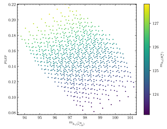
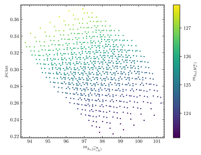
Figure 9: Values for $\mu_{\mathrm{LEP}}$ (top) and for $\mu_{\mathrm{CMS}}$ (bottom) for each parameter point versus the mass of $\widetilde{\nu}_{\tau R}^{\mathcal{R}}$. The colors indicate the mass of the SM-like Higgs boson.

In Fig. 9 we show the results for the signal strength of the LEP excess $\mu_{\mathrm{LEP}}$ (top) and of the CMS excess $\mu_{\mathrm{CMS}}$ (bottom). In both plots the colors of the points indicate the SM-like Higgs-boson mass, while the mass of $\widetilde{\nu}_{\tau R}^{\mathcal{R}}$ is shown on the horizontal axis. The signal strengths were calculated in the narrow-width approximation, and the branching ratio and cross section ratios w.r.t. the SM where calculated using the effective coupling approximation as explained in Ref. [99]. One can immediately see that it is rather easy to achieve the experimental value of $\mu_{\mathrm{LEP}}$, whereas the largest values for $\mu_{\mathrm{CMS}}$ reached in our scan are just below the lower limit of $\mu_{\mathrm{CMS}}=0.4$, i.e., $1\sigma$ below the central value. This is due to the fact that the main decay channel of $\widetilde{\nu}_{\tau R}^{\mathcal{R}}$ is the decay to a pair of bottom quarks, and it is harder to achieve a substantial branching ratio to diphotons required for the CMS excess. Nevertheless, both excesses are fitted at the $1\sigma$ level considering the experimental uncertainties, while fitting the neutrino data and being in agreement with the experimental constraints on the SM-like Higgs boson, which we again checked with HiggsSignals assuming a theoretical uncertainty of the SM-like Higgs-boson mass of $3\,\,\mathrm{GeV}$.

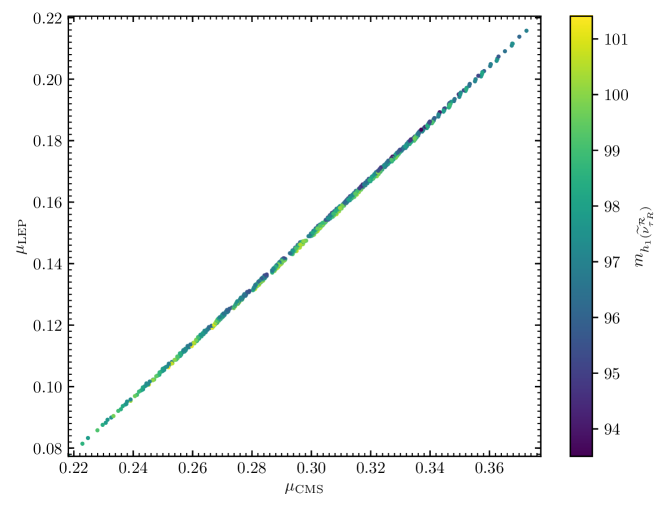
Figure 10: Correlation of both signal strengths, with the colors encoding the mass of $\widetilde{\nu}_{\tau R}^{\mathcal{R}}$.

In Fig. 10 we show the correlation of both signal strengths, with the colors encoding the mass of $\widetilde{\nu}_{\tau R}^{\mathcal{R}}$. The strong correlation one can see has its origin in the fact that both signal strengths increase with the amount of doublet-component of $\widetilde{\nu}_{\tau R}^{\mathcal{R}}$. In principle, one could achieve a further enhancement of $\mu_{\mathrm{CMS}}$ and a suppression of $\mu_{\mathrm{LEP}}$ by suppressing the down-type doublet component of $\widetilde{\nu}_{\tau R}^{\mathcal{R}}$. Then, the branching ratio to bottom quarks becomes smaller, and the diphoton branching ratio increases because of the smaller total decay width due to the reduction of the decay width to bottom quarks. However, finding such points is difficult, because the dominant terms mixing the right-handed sneutrinos $\widetilde{\nu}_{iR}^{\mathcal{R}}$ with the doublet fields $H_{d}^{\mathcal{R}}$ and $H_{u}^{\mathcal{R}}$ scale equally with $\lambda_{i}$, $A^{\lambda}_{i}$, $\kappa_{ijk}$ and $v_{iR}$ at tree level, as can be seen in Eqs. (A.4) and (A.5). The only difference are the factors $v_{d}$ and $v_{u}$ in each equation, respectively, which cannot be exploited too much, because, as mentioned before, $\tan\beta$ should not be too far from one. This is why an extensive scan of the vast parameter space of the $\mu\nu\mathrm{SSM}$ would be necessary to find parameter points in which $\mu_{\mathrm{CMS}}$ is further enhanced without increasing $\mu_{\mathrm{LEP}}$ too much, which however lies beyond the scope of this paper.

Instead, we will focus on the rest of the spectrum, which heavily depends on the values of the neutrino Yukawa couplings $Y^{\nu}_{ij}$ and the vevs of the left-handed sneutrinos $v_{iL}$, once the remaining parameters are fixed to the values listed in Tab. 5. As an example, we show in Tab. 6 two possible sets of parameters that accommodate accurate neutrino masses and mixings in the parameter scan of this section. In contrast to the other scenarios we presented before, here we will make use of non-zero values of the non-diagonal elements of $Y^{\nu}_{ij}$ in one of the BPs. Naturally, this simplifies the accommodation of neutrino properties in agreement with experimental data, because there are six more free parameters that can be adjusted. The price to pay is that there is usually more than one set of parameters of $Y^{\nu}_{ij}$ and $v_{iL}$ that give accurate predictions for the neutrino sector. The reason for showing two distinct scenarios is that in the $\mu\nu\mathrm{SSM}$ the scalar sector is deeply related to the neutrino sector. Thus, different sets of parameters predict fundamentally different scalar spectra, and since there is no theoretical argument that the neutrino Yukawa couplings have to be diagonal, we used the additional freedom to present a point in which, on top of the explanation of the LEP and the CMS excesses, there are a several other light particles possibly in reach of future colliders.

	$Y^{\nu}_{11}$	$Y^{\nu}_{12}$	$Y^{\nu}_{13}$	$Y^{\nu}_{21}$	$Y^{\nu}_{22}$	$Y^{\nu}_{23}$
BP1	$8.109\cdot 10^{-8}$	$0$	$0$	$0$	$1.154\cdot 10^{-7}$	$0$
BP2	$7.088\cdot 10^{-8}$	$1.181\cdot 10^{-8}$	$-3.404\cdot 10^{-9}$	$1.902\cdot 10^{-8}$	$1.238\cdot 10^{-7}$	$1.783\cdot 10^{-8}$
	$Y^{\nu}_{31}$	$Y^{\nu}_{32}$	$Y^{\nu}_{33}$	$v_{1L}$	$v_{2L}$	$v_{3L}$
BP1	$0$	$0$	$8.855\cdot 10^{-7}$	$1.890\cdot 10^{-5}$	$2.601\cdot 10^{-4}$	$1.871\cdot 10^{-4}$
BP2	$-2.103\cdot 10^{-9}$	$6.923\cdot 10^{-9}$	$1.383\cdot 10^{-8}$	$1.792\cdot 10^{-6}$	$2.072\cdot 10^{-4}$	$3.673\cdot 10^{-4}$
BP1	$m_{\lambda_{4}}(\nu_{\tau R})$	$m_{A_{1}}(\widetilde{\nu}_{\tau R}^{\mathcal{I}})$	$m_{H^{+}_{1}}(\widetilde{\mu}_{L})$	$m_{A_{2}}(\widetilde{\nu}_{\mu L}^{\mathcal{I}})$	$m_{h_{3}}(\widetilde{\nu}_{\mu L}^{\mathcal{R}})$	$m_{\lambda_{5}}(\widetilde{H}_{d,u})$
	78	97-109	283	285	285	$323-326$
BP2	$m_{\lambda_{4}}(\nu_{\tau R})$	$m_{h_{1}}(\widetilde{\nu}_{\tau L}^{\mathcal{R}})$	$m_{A_{1}}(\widetilde{\nu}_{\tau L}^{\mathcal{I}})$	$m_{H^{+}_{1}}(\widetilde{\tau}_{L})$	$m_{A_{2}}(\widetilde{\nu}_{\tau R}^{\mathcal{I}})$	$m_{\lambda_{5}}(\widetilde{H}_{d,u})$
	78	79	79	98	97-109	$323-326$

Table 6: Parameter sets BP1 and BP2 used to fit the neutrino oscillation data accurately in the scan reproducing the LEP and the CMS excesses. In the last four rows we list the masses of the six lightest non-SM particles (in addition to $\widetilde{\nu}_{\tau R}^{\mathcal{R}}$ at $\sim 96\,\,\mathrm{GeV}$) for each BP. Dimensionful parameters are given in GeV.

In both BPs the lightest BSM particle is the right-handed $\tau$-neutrino. This is because $\kappa_{333}$ has to be small to decrease the mass of the corresponding sneutrino $\widetilde{\nu}_{\tau R}^{\mathcal{R}}$. Consequently, also the Majorana mass term for the neutrino will be small and $m_{\nu_{\tau R}}$ is small. However, its mass is still above half the SM-like Higgs-boson mass, so the decay of the SM-like Higgs boson into $\nu_{\tau R}$ is forbidden. The striking difference between both BPs is the mass scale of the left-handed $\tau$-sneutrinos and sleptons. In BP2 the Yukawa coupling $Y^{\nu}_{33}$ is the smallest diagonal element of $Y^{\nu}$, and the vev corresponding to the third family of left-handed sneutrinos $v_{3L}$ is the largest of the three. This reduces the masses of the left-handed ${{\cal CP}}$-even and ${{\cal CP}}$-odd $\tau$-sneutrino (see Eq. (2.31)) and the $\tau$-slepton to values below the SM-like Higgs-boson mass. In BP1, on the other hand, $v_{2L}$ is the largest of the three left-handed vevs, and therefore the left-handed $\mu$-sneutrinos and $\mu$-slepton are the lightest left-handed sfermions, although still more than twice as heavy as the SM-like Higgs boson. In this way, the phenomenology of both BPs is distinct, even though the properties of the right-handed $\tau$-sneutrino, which is the particle used to fit the excesses, are not affected by the left-handed sector. This is because its branching ratios are dominantly given by the mixing-effects with the SM-like Higgs boson, which is not suppressed by the small neutrino Yukawa couplings $Y^{\nu}_{ij}$.

Nonetheless, BP2 can give rise to additional interesting signal at colliders. A dedicated analysis of the collider phenomenology of light left-handed $\tau$-sneutrinos/sleptons at the LHC can be found in Refs. [29, 30], where it was shown that there are no direct bounds from LEP/LHC searches that can be used to set lower limits on the masses of these particles in the framework of the $\mu\nu\mathrm{SSM}$. This analysis made use of the fact that the charged $\widetilde{\tau}_{L}$ can be produced, and thus provide a source for the left-handed sneutrinos, since it decays into lighter $\widetilde{\nu}_{\tau L}^{\mathcal{R}}$ or $\widetilde{\nu}_{\tau L}^{\mathcal{I}}$. An important feature is that the subsequent decays of $\widetilde{\nu}_{\tau L}^{\mathcal{R,I}}$ can be prompt or displaced. However, in Refs. [29, 30] it is assumed that the left-handed sneutrino is the LSP. This is not the case here, since the right-handed $\tau$-neutrino is even lighter. Signals at colliders from the lightest BSM particle $\nu_{\tau R}$ are not expected, because it is a gauge singlet, thus cannot be produced directly. In principle, it can be produced indirectly via the decay of the sfermions. However, the spectrum is very compressed, such that a pair production of $\nu_{\tau R}$ from the decays of $\widetilde{\nu}_{\tau R}$ at $\sim 96\,\,\mathrm{GeV}$ or the SM-like Higgs boson at $\sim 125\,\,\mathrm{GeV}$ is kinematically forbidden, and the production of a pair of a right- and a left-handed $\tau$-neutrino is suppressed by the size of $Y^{\nu}_{33}$.

6 Conclusion and Outlook

The $\mu\nu\mathrm{SSM}$ is a simple SUSY extension of the SM that is capable of describing neutrino physics in agreement with experimental data. As in other SUSY models, higher-order corrections are crucial to reach a theoretical uncertainty at the same level of the (anticipated) experimental accuracy. So far, higher-order corrections in the $\mu\nu\mathrm{SSM}$ had been restricted to $\smash{\overline{\mathrm{DR}}}$ calculations, which suffer from the disadvantage that they cannot be directly connected to (possibly future observed) new BSM particles. More recently we had evaluated the corrections to the neutral scalar masses and mixings, but restricting ourselves to one generation of heavy neutrinos [99].

In this paper we have presented the complete one-loop renormalization of the neutral scalar sector of the $\mu\nu\mathrm{SSM}$ with three generation of right-handed neutrinos in a mixed on-shell/$\smash{\overline{\mathrm{DR}}}$ scheme. In this way, for the first time, it is possible to evaluate the masses and mixings in the neutral scalar sector with high precision, while simultaneously describe correctly the experimental neutrino data, such as mass differences and mixing angles. An on-shell (OS) renormalization has been chosen for parameters that can be directly identified with (potentially) observable states, whereas a $\smash{\overline{\mathrm{DR}}}$ renormalization has been chosen for the remaining parameters. We provide details on the full set renormalization parameters, which were implemented into a FeynArts model file (that can be provided by the authors upon request).

We have performed the calculation of the masses of the neutral scalars in the $\mu\nu\mathrm{SSM}$ with three generations of heavy neutrinos, taking into account the full set of one-loop corrections as described above. These corrections have been supplemented by contributions to the neutral Higgs-boson sector of the MSSM at and beyond the two-loop level as provided by FeynHiggs. These corrections are crucial to obtain a reliable prediction of the mass of an SM-like Higgs boson around $\sim 125\,\,\mathrm{GeV}$.

The masses of the neutral scalar bosons have been evaluated in a set of scenarios that exemplify the relevant dependences on the underlying $\mu\nu\mathrm{SSM}$ parameters. The scenarios are in agreement with all available searches for additional Higgs bosons (via the code HiggsBounds), as well with the properties of the SM-like Higgs boson as measured at the LHC (via the code HiggsSignals), while at the same time reproducing correctly the measured values of neutrino mass differences and mixing angles. In a first scenario we varied the assumed to be universal parameter $\lambda$. We find that large one-loop corrections for the right-handed sneutrinos arise, that are crucial to accurately account for possible mixing effects between them and the SM-like Higgs boson. In a second scenario we have varied the assumed to be universal vev of the right-handed sneutrinos. Here we find that all three ${{\cal CP}}$-even right-handed sneutrinos can have masses below $\sim 125\,\,\mathrm{GeV}$, without being excluded by cross-section limits from direct searches for additional Higgs bosons. In our third scenario we deviate from the intergenerational universality assumptions. We take $\boldsymbol{\lambda}^{2}\mathrel{\mathop{\mathchar 58\relax}}=\lambda_{i}\lambda_{i}$ to be constant, but vary instead the individual $\lambda_{i}$. We find that the non-universality of the $\lambda_{i}$ has an important impact on the predictions of the neutral scalar masses. It has been shown that in the experimentally allowed parameter space the non-universality of the $\lambda_{i}$ can account for deviations of the SM-like Higgs-boson mass of $\sim 1\,\,\mathrm{GeV}$, emphasizing the importance to consider the full set of $\mu\nu\mathrm{SSM}$ parameters at the one-loop level.

As a final example we have discussed how the $\mu\nu\mathrm{SSM}$ can describe two excesses in the searches for light Higgs bosons in the vicinity of $\sim 96\,\,\mathrm{GeV}$. These are a $\sim 3\,\sigma$ excess in the diphoton final state as reported by CMS and a $\sim 2\,\sigma$ excess in the $b\bar{b}$ final state as published by LEP. We demonstrated that the $\mu\nu\mathrm{SSM}$ can account at the $\sim 1\,\sigma$ level for both excesses, while being in agreement with all available Higgs-boson searches and measurements, as well as the available neutrino data. We are eagerly awaiting updated experimental analyses from ATLAS and CMS to confirm or refute these excesses.

Further explorations of the scalar sector of the $\mu\nu\mathrm{SSM}$ are necessary to cover the wealth of (possible) phenomenology that this model offers. This includes further studies dropping the (artificial) intergenerational universality assumptions, where in this paper we have taken only the first step. It furthermore includes the evaluation of the charged scalar sector at the one-loop level and beyond, which is expected to be important for the phenomenology at the LHC. Also studies going beyond the LHC searches may become relevant, such as analyses of the possibility of a first order phase transition, leading to gravitational waves created in the early universe. We leave these studies for future work.

Acknowledgements

We thank Daniel E. Lopez-Fogliani for helpful discussions concerning the neutrino physics. This work was supported in part by the Spanish Agencia Estatal de Investigación through the grants FPA2016-78022-P MINECO/FEDER-UE (TB and SH), FPA2015-65929-P MINECO/FEDER-UE and PGC2018-095161-B-I00 (CM), by the “Spanish Red Consolider MultiDark” FPA2017-90566-REDC, and IFT Centro de Excelencia Severo Ochoa SEV-2016-0597. The work of TB was funded by Fundación La Caixa under ‘La Caixa-Severo Ochoa’ international predoctoral grant.

Appendix A Mass matrices

Here we give the entries of the following scalar mass matrices.

A.1 ${{\cal CP}}$-even scalars

In the interaction basis $\varphi^{T}=(H_{d}^{\mathcal{R}},H_{u}^{\mathcal{R}},\widetilde{\nu}_{iR}^{\mathcal{R}},\widetilde{\nu}_{jL}^{\mathcal{R}})$ the mass matrix for the ${{\cal CP}}$-even scalars $m_{\varphi}^{2}$ is defined by:

$$m_{H_{d}^{\mathcal{R}}H_{d}^{\mathcal{R}}}^{2} =m_{H_{d}}^{2}+\frac{1}{8}\left(g_{1}^{2}+g_{2}^{2}\right)\left(3v_{d}^{2}+v_{iL}v_{iL}-v_{u}^{2}\right)+\frac{1}{2}\left(v_{u}^{2}\lambda_{i}\lambda_{i}+\left(v_{iR}\lambda_{i}\right)^{2}\right)\;,$$ (A.1)

$$m_{H_{u}^{\mathcal{R}}H_{u}^{\mathcal{R}}}^{2} =m_{H_{u}}^{2}+\frac{1}{8}\left(g_{1}^{2}+g_{2}^{2}\right)\left(3v_{u}^{2}-v_{d}^{2}-v_{iL}v_{iL}\right)+\frac{1}{2}\lambda_{i}\lambda_{i}v_{d}^{2}-v_{d}Y^{\nu}_{ji}\lambda_{i}v_{jL}$$

$$+\frac{1}{2}\left(v_{iR}\lambda_{i}\right)^{2}+\frac{1}{2}Y^{\nu}_{ji}Y^{\nu}_{ki}v_{jL}v_{kL}+\frac{1}{2}Y^{\nu}_{ij}Y^{\nu}_{ik}v_{jR}v_{kR}\;,$$ (A.2)

$$m_{H_{u}^{\mathcal{R}}H_{d}^{\mathcal{R}}}^{2} =-\frac{1}{4}\left(g_{1}^{2}+g_{2}^{2}\right)v_{d}v_{u}+v_{d}v_{u}\lambda_{i}\lambda_{i}-\frac{1}{\sqrt{2}}T^{\lambda}_{i}v_{iR}-v_{u}Y^{\nu}_{ji}\lambda_{i}v_{jL}-\frac{1}{2}\kappa_{ijk}\lambda_{i}v_{jR}v_{kR}\;,$$ (A.3)

$$m_{\widetilde{\nu}^{\mathcal{R}}_{iR}H_{d}^{\mathcal{R}}}^{2} =-v_{u}\kappa_{ijk}\lambda_{j}v_{kR}-\frac{1}{2}v_{jR}\lambda_{j}v_{kL}Y^{\nu}_{ki}+v_{d}v_{jR}\lambda_{j}\lambda_{i}-\frac{1}{2}v_{jL}Y^{\nu}_{jk}v_{kR}\lambda_{i}-\frac{1}{\sqrt{2}}v_{u}T^{\lambda}_{i}\;,$$ (A.4)

$$m_{\widetilde{\nu}^{\mathcal{R}}_{iR}H_{u}^{\mathcal{R}}}^{2} =\frac{1}{\sqrt{2}}v_{jL}T^{\nu}_{ji}+v_{u}Y^{\nu}_{ji}Y^{\nu}_{jk}v_{kR}-v_{d}\kappa_{ijk}\lambda_{j}v_{kR}+Y^{\nu}_{lj}\kappa_{ijk}v_{kR}v_{lL}+v_{u}v_{jR}\lambda_{j}\lambda_{i}-\frac{1}{\sqrt{2}}v_{d}T^{\lambda}_{i}\;,$$ (A.5)

$$m_{\widetilde{\nu}^{\mathcal{R}}_{iR}\widetilde{\nu}^{\mathcal{R}}_{jR}}^{2} =\left(m_{\widetilde{v}_{R}}^{2}\right)_{ij}+\frac{1}{2}v_{u}^{2}Y^{\nu}_{ki}Y^{\nu}_{kj}-v_{d}v_{u}\kappa_{ijk}\lambda_{k}+\sqrt{2}v_{kR}T^{\kappa}_{ijk}+v_{u}Y^{\nu}_{lk}\kappa_{ijk}v_{lL}+\frac{1}{2}v_{kL}Y^{\nu}_{ki}v_{lL}Y^{\nu}_{lj}$$

$$+2\kappa_{ikl}\kappa_{jkm}v_{lR}v_{mR}+\kappa_{ijk}\kappa_{klm}v_{lR}v_{mR}-\frac{1}{2}v_{d}v_{kL}Y^{\nu}_{kj}\lambda_{i}-\frac{1}{2}v_{d}v_{kL}Y^{\nu}_{ki}\lambda_{j}$$

$$+\frac{1}{2}\left(v_{d}^{2}+v_{u}^{2}\right)\lambda_{i}\lambda_{j}\;,$$ (A.6)

$$m_{\widetilde{\nu}_{iL}^{\mathcal{R}}H_{d}^{\mathcal{R}}}^{2} =\left(m_{H_{d}\widetilde{L}}^{2}\right)_{i}+\frac{1}{4}\left(g_{1}^{2}+g_{2}^{2}\right)v_{d}v_{iL}-\frac{1}{2}v_{u}^{2}Y^{\nu}_{ij}\lambda_{j}-\frac{1}{2}v_{jR}\lambda_{j}v_{kR}Y^{\nu}_{ik}\;,$$ (A.7)

$$m_{\widetilde{\nu}_{iL}^{\mathcal{R}}H_{u}^{\mathcal{R}}}^{2} =-\frac{1}{4}\left(g_{1}^{2}+g_{2}^{2}\right)v_{u}v_{iL}-v_{d}v_{u}Y^{\nu}_{ij}\lambda_{j}+\frac{1}{\sqrt{2}}v_{jR}T^{\nu}_{ij}+v_{u}Y^{\nu}_{ij}Y^{\nu}_{kj}v_{kL}+\frac{1}{2}Y^{\nu}_{ij}\kappa_{jkl}v_{kR}v_{lR}\;,$$ (A.8)

$$m_{\widetilde{\nu}_{iR}^{\mathcal{R}}\widetilde{\nu}^{\mathcal{R}}_{jL}}^{2} =v_{u}Y^{\nu}_{jk}\kappa_{ikl}v_{lR}+\frac{1}{2}v_{kL}Y^{\nu}_{ki}v_{lR}Y^{\nu}_{jl}-\frac{1}{2}v_{d}v_{kR}\lambda_{k}Y^{\nu}_{ji}+\frac{1}{2}v_{kL}Y^{\nu}_{kl}v_{lR}Y^{\nu}_{ji}\;,$$

$$-\frac{1}{2}v_{d}v_{kR}Y^{\nu}_{jk}\lambda_{i}+\frac{1}{\sqrt{2}}v_{u}T^{\nu}_{ji}\;,$$ (A.9)

$$m_{\widetilde{\nu}_{iL}^{\mathcal{R}}\widetilde{\nu}_{jL}^{\mathcal{R}}}^{2} =\left(m_{\widetilde{L}}^{2}\right)_{ij}+\frac{1}{8}\delta_{ij}\left(g_{1}^{2}+g_{2}^{2}\right)\left(v_{d}^{2}-v_{u}^{2}+v_{kL}v_{kL}\right)+\frac{1}{4}\left(g_{1}^{2}+g_{2}^{2}\right)v_{iL}v_{jL}$$

$$+\frac{1}{2}v_{u}^{2}Y^{\nu}_{ik}Y^{\nu}_{jk}+\frac{1}{2}v_{kR}Y^{\nu}_{jk}v_{lR}Y^{\nu}_{il}\;.$$ (A.10)

A.2 ${{\cal CP}}$-odd scalars

In the interaction basis $\sigma^{T}=(H_{d}^{\mathcal{I}},H_{u}^{\mathcal{I}},\widetilde{\nu}_{iR}^{\mathcal{I}},\widetilde{\nu}_{jL}^{\mathcal{I}})$ the mass matrix for the ${{\cal CP}}$-odd scalars $m_{\sigma}^{2}$ is defined by:

$$m_{H_{d}^{\mathcal{I}}H_{d}^{\mathcal{I}}}^{2} =m_{H_{d}}^{2}+\frac{1}{8}\left(g_{1}^{2}+g_{2}^{2}\right)\left(v_{d}^{2}+v_{iL}v_{iL}-v_{u}^{2}\right)+\frac{1}{2}\left(v_{u}^{2}\lambda_{i}\lambda_{i}+\left(v_{iR}\lambda_{i}\right)^{2}\right)\;,$$ (A.11)

$$m_{H_{u}^{\mathcal{I}}H_{u}^{\mathcal{I}}}^{2} =m_{H_{u}}^{2}+\frac{1}{8}\left(g_{1}^{2}+g_{2}^{2}\right)\left(v_{u}^{2}-v_{d}^{2}-v_{iL}v_{iL}\right)+\frac{1}{2}v_{d}^{2}\lambda_{i}\lambda_{i}-v_{d}Y^{\nu}_{ji}\lambda_{i}v_{jL}+\frac{1}{2}\left(v_{iR}\lambda_{i}\right)^{2}$$

$$+\frac{1}{2}Y^{\nu}_{ji}Y^{\nu}_{ki}v_{jL}v_{kL}+\frac{1}{2}Y^{\nu}_{ij}Y^{\nu}_{ik}v_{jR}v_{kR}\;,$$ (A.12)

$$m_{H_{u}^{\mathcal{I}}H_{d}^{\mathcal{I}}}^{2} =\frac{1}{2}\kappa_{ijk}\lambda_{i}v_{jR}v_{kR}+\frac{1}{\sqrt{2}}v_{iR}T^{\lambda}_{i}\;,$$ (A.13)

$$m_{\widetilde{{\nu}}^{\mathcal{I}}_{iR}H_{d}^{\mathcal{I}}}^{2} =v_{u}\kappa_{ijk}\lambda_{j}v_{kR}+\frac{1}{2}v_{jR}\lambda_{j}v_{kL}Y^{\nu}_{ki}-\frac{1}{2}v_{jL}Y^{\nu}_{jk}v_{kR}\lambda_{i}-\frac{1}{\sqrt{2}}v_{u}T^{\lambda}_{i}\;,$$ (A.14)

$$m_{\widetilde{{\nu}}^{\mathcal{I}}_{iR}H_{u}^{\mathcal{I}}}^{2} =\frac{1}{\sqrt{2}}v_{jL}T^{\nu}_{ji}+v_{d}\kappa_{ijk}\lambda_{j}v_{kR}-Y^{\nu}_{lj}\kappa_{ijk}v_{kR}v_{lL}-\frac{1}{\sqrt{2}}v_{d}T^{\lambda}_{i}\;,$$ (A.15)

$$m_{\widetilde{{\nu}}^{\mathcal{I}}_{iR}\widetilde{{\nu}}^{\mathcal{I}}_{jR}}^{2} =\left(m_{\widetilde{\nu}}^{2}\right)_{ij}+\frac{1}{2}v_{u}^{2}Y^{\nu}_{ki}Y^{\nu}_{kj}+v_{d}v_{u}\kappa_{ijk}\lambda_{k}-\sqrt{2}v_{kR}T^{\kappa}_{ijk}-v_{u}Y^{\nu}_{lk}\kappa_{ijk}v_{lL}+\frac{1}{2}v_{kL}Y^{\nu}_{ki}v_{lL}Y^{\nu}_{lj}$$

$$+\kappa_{ikm}\kappa_{jkl}v_{lR}v_{mR}-\kappa_{ijk}\kappa_{klm}v_{lR}v_{mR}-\frac{1}{2}v_{d}v_{kL}Y^{\nu}_{kj}\lambda_{i}-\frac{1}{2}v_{d}v_{kL}Y^{\nu}_{ki}\lambda_{j}$$

$$+\frac{1}{2}\left(v_{d}^{2}+v_{u}^{2}\right)\lambda_{i}\lambda_{j}\;,$$ (A.16)

$$m_{\widetilde{\nu}_{iL}^{\mathcal{I}}H_{d}^{\mathcal{I}}}^{2} =\left(m_{H_{d}\widetilde{L}}^{2}\right)_{i}-\frac{1}{2}v_{u}^{2}Y^{\nu}_{ij}\lambda_{j}-\frac{1}{2}v_{jR}\lambda_{j}v_{kR}Y^{\nu}_{ik}\;,$$ (A.17)

$$m_{\widetilde{\nu}_{iL}^{\mathcal{I}}H_{u}^{\mathcal{I}}}^{2} =-\frac{1}{\sqrt{2}}v_{jR}T^{\nu}_{ij}-\frac{1}{2}Y^{\nu}_{ij}\kappa_{jkl}v_{kR}v_{lR}\;,$$ (A.18)

$$m_{\widetilde{\nu}_{iR}^{\mathcal{I}}\widetilde{\nu}^{\mathcal{I}}_{jL}}^{2} =-v_{u}Y^{\nu}_{jk}\kappa_{ikl}v_{lR}-\frac{1}{2}v_{kL}Y^{\nu}_{ki}v_{lR}Y^{\nu}_{jl}-\frac{1}{2}v_{d}v_{kR}\lambda_{k}Y^{\nu}_{ji}+\frac{1}{2}v_{kL}Y^{\nu}_{kl}v_{lR}Y^{\nu}_{ji}$$

$$+\frac{1}{2}v_{d}v_{kR}Y^{\nu}_{jk}\lambda_{i}+\frac{1}{\sqrt{2}}v_{u}T^{\nu}_{ji}\;,$$ (A.19)

$$m_{\widetilde{\nu}_{iL}^{\mathcal{I}}\widetilde{\nu}_{jL}^{\mathcal{I}}}^{2} =\left(m_{\widetilde{L}}^{2}\right)_{ij}+\frac{1}{8}\delta_{ij}\left(g_{1}^{2}+g_{2}^{2}\right)\left(v_{d}^{2}+v_{kL}v_{kL}-v_{u}^{2}\right)+\frac{1}{2}v_{u}^{2}Y^{\nu}_{ik}Y^{\nu}_{jk}+\frac{1}{2}v_{kR}Y^{\nu}_{ik}v_{lR}Y^{\nu}_{jl}\;.$$ (A.20)

A.3 Charged scalars

In the gauge eigenstate basis $C^{T}=({H^{-}_{d}}^{*},{H^{+}_{u}},\widetilde{e}_{iL}^{*},\widetilde{e}_{jR}^{*})$ the entries of $m_{H^{+}}^{2}$ are given by:

$$m_{H_{d}^{-}{H^{-}_{d}}^{*}}^{2} =m_{H_{d}}^{2}+\frac{1}{8}g_{1}^{2}\left(v_{d}^{2}+v_{iL}v_{iL}-v_{u}^{2}\right)+\frac{1}{8}g_{2}^{2}\left(v_{d}^{2}-v_{iL}v_{iL}+v_{u}^{2}\right)+\frac{1}{2}\left(v_{iR}\lambda_{i}\right)^{2}$$

$$+\frac{1}{2}Y^{e}_{ij}Y^{e}_{ik}v_{jL}v_{kL}\;,$$ (A.21)

$$m_{{H_{u}^{+}}^{*}{H_{u}^{+}}}^{2} =m_{H_{u}}^{2}+\frac{1}{8}g_{1}^{2}\left(v_{u}^{2}-v_{d}^{2}-v_{iL}v_{iL}\right)+\frac{1}{8}g_{2}^{2}\left(v_{u}^{2}+v_{d}^{2}+v_{iL}v_{iL}\right)+\frac{1}{2}\left(v_{iR}\lambda_{i}\right)^{2}$$

$$+\frac{1}{2}Y^{\nu}_{ij}Y^{\nu}_{ik}v_{jR}v_{kL}\;,$$ (A.22)

$$m_{H_{d}^{-}{H^{+}_{u}}}^{2} =\frac{1}{4}g_{2}^{2}v_{d}v_{u}-\frac{1}{2}v_{d}v_{u}\lambda_{i}\lambda_{i}+\frac{1}{\sqrt{2}}v_{iR}T^{\lambda}_{i}+\frac{1}{2}v_{u}Y^{\nu}_{ji}\lambda_{i}v_{jL}+\frac{1}{2}\kappa_{ijk}\lambda_{i}v_{jR}v_{kR}\;,$$ (A.23)

$$m_{{{H^{-}_{d}}}{\widetilde{e}_{iL}}^{*}}^{2} =\left(m_{H_{d}\widetilde{L}}^{2}\right)_{i}+\frac{1}{4}g_{2}^{2}v_{d}v_{iL}-\frac{1}{2}v_{d}Y^{e}_{ji}Y^{e}_{jk}v_{kL}-\frac{1}{2}v_{jR}Y^{\nu}_{ij}v_{kR}\lambda_{k}\;,$$ (A.24)

$$m_{{H_{u}^{+}}^{*}{\widetilde{e}_{iL}}^{*}}^{2} =\frac{1}{4}g_{2}^{2}v_{u}v_{iL}+\frac{1}{2}v_{d}v_{u}Y^{\nu}_{ij}\lambda_{j}-\frac{1}{\sqrt{2}}v_{jR}T^{\nu}_{ij}-\frac{1}{2}v_{u}Y^{\nu}_{ij}Y^{\nu}_{kj}v_{kL}-\frac{1}{2}Y^{\nu}_{ij}\kappa_{jkl}v_{kR}v_{lR}\;,$$ (A.25)

$$m_{{{H^{-}_{d}}}{\widetilde{e}_{iR}}^{*}}^{2} =-\frac{1}{\sqrt{2}}v_{jL}T^{e}_{ij}-\frac{1}{2}v_{u}Y^{e}_{ij}Y^{\nu}_{jk}v_{jR}\;,$$ (A.26)

$$m_{{H_{u}^{+}}^{*}{\widetilde{e}_{iR}}^{*}}^{2} =-\frac{1}{2}v_{d}Y^{e}_{ij}Y^{\nu}_{jk}v_{kR}-\frac{1}{2}v_{jR}\lambda_{j}v_{kL}Y^{e}_{ik}\;,$$ (A.27)

$$m_{\widetilde{e}_{iL}\widetilde{e}_{jL}^{*}}^{2} =\left(m_{\widetilde{L}}^{2}\right)_{ij}+\frac{1}{8}\delta_{ij}\left(g_{1}^{2}-g_{2}^{2}\right)\left(v_{d}^{2}-v_{u}^{2}+v_{kL}v_{kL}\right)+\frac{1}{4}g_{2}^{2}v_{iL}v_{jL}+\frac{1}{2}v_{d}^{2}Y^{e}_{ki}Y^{e}_{kj}$$

$$+\frac{1}{2}v_{kR}Y^{\nu}_{jk}v_{lR}Y^{\nu}_{il}\;,$$ (A.28)

$$m_{\widetilde{e}_{iR}\widetilde{e}_{jR}^{*}}^{2} =\left(m_{\widetilde{e}}^{2}\right)_{ij}+\frac{1}{4}\delta_{ij}g_{1}^{2}\left(v_{u}^{2}-v_{d}^{2}-v_{kL}v_{kL}\right)+\frac{1}{2}v_{d}^{2}Y^{e}_{ik}Y^{e}_{jk}+\frac{1}{2}v_{kL}Y^{e}_{ik}v_{lL}Y^{e}_{jl}\;,$$ (A.29)

$$m_{\widetilde{e}_{iL}\widetilde{e}_{jR}^{*}}^{2} =\frac{1}{\sqrt{2}}v_{d}T^{e}_{ij}-\frac{1}{2}v_{u}v_{kR}\lambda_{k}Y^{e}_{ij}\;.$$ (A.30)

Appendix B Explicit expressions for counterterms

In this section we will state the one-loop counterterms that were calculated diagrammatically in the $\smash{\overline{\mathrm{DR}}}$ scheme and checked against master formulas for the one-loop beta functions and anomalous dimensions of soft SUSY breaking parameters [120, 121, 123], superpotential parameters [122, 123], vacuum expectation values [170] and wave-functions with kinetic mixing [124, 125]. The master formulas were evaluated using the mathematica package SARAH [171].

B.1 Field renormalization counterterms

We list the field renormalization counterterms defined in Eq. (3.25) in the $\smash{\overline{\mathrm{DR}}}$ scheme in the interaction basis $(H_{d},H_{u},\widetilde{\nu}_{1R},\widetilde{\nu}_{2R},\widetilde{\nu}_{3R},\widetilde{\nu}_{1L},\widetilde{\nu}_{2L},\widetilde{\nu}_{3L})$:

$$\delta Z_{11} =-\frac{\Delta}{16\pi^{2}}\left(\lambda_{i}\lambda_{i}+Y^{e}_{ij}Y^{e}_{ij}+3\left(Y^{d}_{i}Y^{d}_{i}\right)\right)\;,$$ (B.1)

$$\delta Z_{1,5+i} =\frac{\Delta}{16\pi^{2}}\lambda_{j}Y^{\nu}_{ij}\;,$$ (B.2)

$$\delta Z_{22} =-\frac{\Delta}{16\pi^{2}}\left(\lambda_{i}\lambda_{i}+Y^{\nu}_{ij}Y^{\nu}_{ij}+3\left(Y^{u}_{i}Y^{u}_{i}\right)\right)\;,$$ (B.3)

$$\delta Z_{2+i,2+j} =-\frac{\Delta}{8\pi^{2}}\left(\lambda_{i}\lambda_{j}+\kappa_{ikl}\kappa_{jkl}+Y^{\nu}_{ki}Y^{\nu}_{kj}\right)\;,$$ (B.4)

$$\delta Z_{5+i,5+j} =-\frac{\Delta}{16\pi^{2}}\left(Y^{e}_{ki}Y^{e}_{kj}+Y^{\nu}_{ik}Y^{\nu}_{jk}\right)\;,$$ (B.5)

where the indices run from 1 to 3. We checked that the coefficients of the divergent part of the field renormalization counterterms are equal to the one-loop anomalous dimensions of the corresponding superfields $\gamma_{ij}^{(1)}$, neglecting the terms proportional to the gauge couplings $g_{1}$ and $g_{2}$, and divided by the loop factor $16\pi^{2}$, i.e.,

$$\delta Z_{ij}=\left.\frac{\gamma_{ij}^{(1)}\Delta}{16\pi^{2}}\right|^{g1,g2\to 0}\;,$$ (B.6)

which is the same relation that holds in the (N)MSSM.

B.2 Parameter counterterms

B.2.1 Renormalization conditions

In the following we list the renormalization conditions for the counterterms of the parameter used to renormalize the neutral scalar potential:

$$\delta g_{2} =\frac{g_{2}}{2}\Biggl{(}\frac{\delta M_{W}^{2}}{M_{W}^{2}}-\frac{\delta v^{2}}{v^{2}}\Biggr{)}\;,$$ (B.7)

$$\delta g_{1} =\frac{2}{g_{1}v^{2}}\left(\delta M_{Z}^{2}-\delta M_{W}^{2}\right)-\frac{g_{1}}{2}\frac{\delta v^{2}}{v^{2}}\;,$$ (B.8)

$$\delta v^{2} =\frac{4s_{\mathrm{w}}^{2}M_{W}^{2}}{e^{2}}\left(\frac{\delta s_{\mathrm{w}}^{2}}{s_{\mathrm{w}}^{2}}+\frac{\delta M_{W}^{2}}{M_{W}^{2}}-2\left.\delta Z_{e}\right|^{\rm div}\right)\;,$$ (B.9)

$$\delta v_{d}^{2} =\frac{4v_{d}}{g_{2}}\Biggl{(}\left.\Sigma_{\widetilde{W}^{0}\widetilde{H}_{d}^{0}}^{S}\right|^{\rm div}-\frac{g_{2}}{4}\biggl{(}v_{d}\bigl{(}\delta Z^{\chi}_{55}+\delta Z^{\chi}_{66}\bigr{)}+v_{iL}\delta Z^{\chi}_{i6}\biggr{)}-\frac{v_{d}}{2}\left.\delta g_{2}\right|^{\rm div}\Biggr{)}\;,$$ (B.10)

$$\delta v_{u}^{2} =\frac{4v_{u}}{g_{2}}\Biggl{(}-\left.\Sigma_{\widetilde{W}^{0}\widetilde{H}_{u}^{0}}^{S}\right|^{\rm div}-\frac{g_{2}v_{u}}{4}\biggl{(}\delta Z^{\chi}_{55}+\delta Z^{\chi}_{77}\biggr{)}-\frac{v_{u}}{2}\left.\delta g_{2}\right|^{\rm div}\Biggr{)}\;,$$ (B.11)

$$\delta Y^{\nu}_{ij} =\frac{\sqrt{2}}{v_{u}}\left.\Sigma_{\nu_{iL}\nu_{jR}^{*}}^{S}\right|^{\rm div}-\frac{1}{2}\left(\delta Z_{ik}^{\chi}Y^{\nu}_{kj}-\delta Z_{i6}^{\chi}\lambda_{j}+\delta Z_{7+k,7+j}^{\chi}Y^{\nu}_{ik}\right)-\frac{Y^{\nu}_{ij}}{2}\frac{\delta v_{u}^{2}}{v_{u}^{2}}\;,$$ (B.12)

$$\delta\lambda_{i} =-\frac{\sqrt{2}}{v_{u}}\left.\Sigma_{\widetilde{H}_{d}^{0}\nu_{iR}^{*}}^{S}\right|^{\rm div}+\frac{1}{2}\left(\delta Z_{j6}^{\chi}Y^{\nu}_{ji}-\delta Z_{66}^{\chi}\lambda_{i}-\delta Z_{7+i,7+j}^{\chi}\lambda_{j}\right)-\frac{\lambda_{i}}{2}\frac{\delta v_{u}^{2}}{v_{u}^{2}}\;,$$ (B.13)

$$\delta v_{iL} =-\frac{2}{g_{1}}\left.\Sigma_{\nu_{iL}\widetilde{B}}^{S}\right|^{\rm div}-\frac{1}{2}\left(\delta Z_{ij}^{\chi}v_{jL}+\delta Z_{i6}^{\chi}v_{d}+\delta Z_{44}^{\chi}v_{iL}\right)-v_{iL}\frac{\delta g_{1}}{g_{1}}\;,$$ (B.14)

$$Y^{\nu}_{ij}\delta v_{jR} =\sqrt{2}\left.\Sigma_{\nu_{iL}\widetilde{H}^{0}_{u}}^{S}\right|^{\rm div}-\frac{1}{2}\left(\delta Z_{ij}^{\chi}v_{kR}Y^{\nu}_{jk}-\delta Z_{i6}^{\chi}v_{jR}\lambda_{j}+\delta Z_{77}^{\chi}v_{jR}Y^{\nu}_{ij}\right)-v_{jR}\delta Y^{\nu}_{ij}\;,$$ (B.15)

$$-v_{u}Y^{\nu}_{jk}\delta\kappa_{iij} =\left.\Gamma_{\widetilde{\nu}_{iR}^{\mathcal{R}}\widetilde{\nu}_{iR}^{\mathcal{R}}\widetilde{\nu}_{jL}^{\mathcal{R}}}^{(1)}\right|^{\rm div}-\frac{1}{2}\biggl{(}2\delta Z_{2+k,2+i}\Gamma_{\widetilde{\nu}_{kR}^{\mathcal{R}}\widetilde{\nu}_{iR}^{\mathcal{R}}\widetilde{\nu}_{jL}^{\mathcal{R}}}^{(0)}+\delta Z_{1,5+j}\Gamma_{\widetilde{\nu}_{iR}^{\mathcal{R}}\widetilde{\nu}_{iR}^{\mathcal{R}}H_{d}^{\mathcal{R}}}^{(0)}$$

$$+\delta Z_{5+k,5+j}\Gamma_{\widetilde{\nu}_{iR}^{\mathcal{R}}\widetilde{\nu}_{iR}^{\mathcal{R}}\widetilde{\nu}_{kL}^{\mathcal{R}}}^{(0)}\biggr{)}-\biggl{(}\lambda_{i}Y^{\nu}_{ji}\delta v_{d}+v_{d}Y^{\nu}_{ji}\delta\lambda_{i}+v_{d}\lambda_{i}\delta Y^{\nu}_{32}-v_{u}\kappa_{iik}\delta Y^{\nu}_{jk}$$

$$-\kappa_{iik}Y^{\nu}_{jk}\delta v_{u}-v_{u}Y^{\nu}_{jk}\delta\kappa_{iik}-v_{kL}Y^{\nu}_{ki}\delta Y^{\nu}_{ji}-v_{kL}Y^{\nu}_{ji}\delta Y^{\nu}_{ki}-Y^{\nu}_{ji}Y^{\nu}_{ki}\delta v_{kL}\biggr{)}\;,$$ (B.16)

$$\delta\kappa_{123} =\frac{\sqrt{2}}{v_{1R}}\left.\Sigma_{\nu_{2R}\nu_{3R}}^{S}\right|^{\rm div}-\frac{1}{2v_{1R}}\biggl{(}\delta Z_{9,7+i}^{\chi}v_{jR}\kappa_{i3j}+v_{jR}\kappa_{i2j}\delta Z_{7+i,10}^{\chi}\biggr{)}$$

$$-\frac{1}{v_{1R}}\biggl{(}v_{2R}\delta\kappa_{223}+v_{3R}\delta\kappa_{233}+\kappa_{i23}\delta v_{iR}\biggr{)}\;,$$ (B.17)

$$\delta T^{\lambda}_{i} =\sqrt{2}\left.\Gamma_{H_{d}^{\mathcal{R}}H_{u}^{\mathcal{R}}\widetilde{\nu}_{iR}^{\mathcal{R}}}^{(1)}\right|^{\rm div}-\frac{1}{\sqrt{2}}\biggl{(}\delta Z_{11}\Gamma_{H_{d}^{\mathcal{R}}H_{u}^{\mathcal{R}}\widetilde{\nu}_{iR}^{\mathcal{R}}}+\delta Z_{5+j,1}\Gamma_{\widetilde{\nu}_{jL}^{\mathcal{R}}H_{u}^{\mathcal{R}}\widetilde{\nu}_{iR}^{\mathcal{R}}}+\delta Z_{22}\Gamma_{H_{d}^{\mathcal{R}}H_{u}^{\mathcal{R}}\widetilde{\nu}_{iR}^{\mathcal{R}}}$$

$$+\delta Z_{2+j,2+i}\Gamma_{H_{d}^{\mathcal{R}}H_{u}^{\mathcal{R}}\widetilde{\nu}_{jR}^{\mathcal{R}}}\biggr{)}-\sqrt{2}\biggl{(}\kappa_{ijk}\lambda_{j}\delta v_{kR}+\kappa_{ijk}v_{kR}\delta\lambda_{j}+\lambda_{j}v_{kR}\delta\kappa_{ijk}\biggr{)}\;,$$ (B.18)

$$\delta T^{\nu}_{ij} =-\sqrt{2}\left.\Gamma_{H_{u}^{\mathcal{R}}\widetilde{\nu}_{iL}^{\mathcal{R}}\widetilde{\nu}_{jR}^{\mathcal{R}}}^{(1)}\right|^{\rm div}+\frac{1}{\sqrt{2}}\biggl{(}\delta Z_{22}\Gamma_{H_{u}^{\mathcal{R}}\widetilde{\nu}_{iL}^{\mathcal{R}}\widetilde{\nu}_{jR}^{\mathcal{R}}}^{(0)}+\delta Z_{2+k,2+j}\Gamma_{H_{u}^{\mathcal{R}}\widetilde{\nu}_{iL}^{\mathcal{R}}\widetilde{\nu}_{kR}^{\mathcal{R}}}^{(0)}$$

$$+\delta Z_{1,5+i}\Gamma_{H_{u}^{\mathcal{R}}H_{d}^{\mathcal{R}}\widetilde{\nu}_{jR}^{\mathcal{R}}}^{(0)}+\delta Z_{5+k,5+i}\Gamma_{H_{u}^{\mathcal{R}}\widetilde{\nu}_{kL}^{\mathcal{R}}\widetilde{\nu}_{jR}^{\mathcal{R}}}^{(0)}\biggr{)}-\sqrt{2}\biggl{(}Y^{\nu}_{ik}\kappa_{jkl}\delta v_{lR}+\kappa_{jkl}v_{lR}\delta Y^{\nu}_{ik}$$

$$+Y^{\nu}_{ik}v_{lR}\delta\kappa_{jkl}\biggr{)}\;,$$ (B.19)

$$\delta T^{\kappa}_{ijk} =-\frac{1}{\sqrt{2}}\left.\Gamma_{\widetilde{\nu}_{iR}^{\mathcal{R}}\widetilde{\nu}_{jR}^{\mathcal{R}}\widetilde{\nu}_{kR}^{\mathcal{R}}}^{(1)}\right|^{\rm div}+\frac{1}{2\sqrt{2}}\biggl{(}\delta Z_{li}\Gamma_{\widetilde{\nu}_{lR}^{\mathcal{R}}\widetilde{\nu}_{jR}^{\mathcal{R}}\widetilde{\nu}_{kR}^{\mathcal{R}}}^{(0)}+\delta Z_{lj}\Gamma_{\widetilde{\nu}_{iR}^{\mathcal{R}}\widetilde{\nu}_{lR}^{\mathcal{R}}\widetilde{\nu}_{kR}^{\mathcal{R}}}^{(0)}+\delta Z_{lk}\Gamma_{\widetilde{\nu}_{iR}^{\mathcal{R}}\widetilde{\nu}_{jR}^{\mathcal{R}}\widetilde{\nu}_{lR}^{\mathcal{R}}}^{(0)}\biggr{)}$$

$$-2\bigl{(}\kappa_{klm}v_{mR}\delta\kappa_{ijl}+\kappa_{ijl}v_{mR}\delta\kappa_{klm}+\kappa_{ijl}\kappa_{klm}\delta v_{mR}+\kappa_{jkl}v_{mR}\delta\kappa_{ilm}$$

$$+\kappa_{ilm}v_{mR}\delta\kappa_{jkl}+\kappa_{ilm}\kappa_{jkl}\delta v_{mR}+\kappa_{jlm}v_{mR}\delta\kappa_{ikl}+\kappa_{ikl}v_{mR}\delta\kappa_{jlm}$$

$$+\kappa_{ikl}\kappa_{jlm}\delta v_{mR}\bigr{)}\;,$$ (B.20)

$$\delta\left(m_{H_{d}\widetilde{L}}^{2}\right)_{i} =\left.\delta\left(m_{\sigma}^{2}\right)_{1,5+i}\right|^{\rm div}+\frac{1}{2}\biggl{(}Y^{\nu}_{ij}\lambda_{j}\delta v_{u}^{2}+v_{u}^{2}\lambda_{j}\delta Y^{\nu}_{ij}+v_{u}^{2}Y^{\nu}_{ij}\delta\lambda_{j}+\lambda_{j}v_{kR}Y^{\nu}_{ik}\delta_{jR}$$

$$+v_{jR}v_{kR}Y^{\nu}_{ik}\delta\lambda_{j}+v_{jR}\lambda_{j}Y^{\nu}_{ik}\delta v_{kR}+v_{jR}\lambda_{j}v_{kR}\delta Y^{\nu}_{ik}\biggr{)}\;,$$ (B.21)

$$\delta\left(m_{\widetilde{\nu}}^{2}\right)_{ij} =\left.\delta\left(m_{\sigma}^{2}\right)_{2+i,2+j}\right|^{\rm div}-\frac{1}{2}\biggl{(}Y^{\nu}_{ki}Y^{\nu}_{kj}\delta v_{u}^{2}+v_{u}^{2}Y^{\nu}_{kj}\delta Y^{\nu}_{ki}+v_{u}^{2}Y^{\nu}_{ki}\delta Y^{\nu}_{kj}\biggr{)}-v_{u}\kappa_{ijk}\lambda_{k}\delta v_{d}$$

$$-v_{d}\kappa_{ijk}\lambda_{k}\delta v_{u}-v_{d}v_{u}\lambda_{k}\delta\kappa_{ijk}-v_{d}v_{d}\kappa_{ijk}\delta\lambda_{k}+\sqrt{2}\biggl{(}T^{\kappa}_{ijk}\delta v_{kR}+v_{kR}\delta T^{\kappa}_{ijk}\biggr{)}$$

$$+Y^{\nu}_{lk}\kappa_{ijk}v_{lL}\delta v_{u}+v_{u}\kappa_{ijk}v_{lL}\delta Y^{\nu}_{lk}+v_{u}Y^{\nu}_{lk}v_{lL}\delta\kappa_{ijk}+v_{u}Y^{\nu}_{lk}\kappa_{ijk}\delta v_{lL}$$

$$-\frac{1}{2}\biggl{(}Y^{\nu}_{ki}v_{lL}Y^{\nu}_{lj}\delta v_{kL}+v_{kL}v_{lL}Y^{\nu}_{lj}\delta Y^{\nu}_{ki}+v_{kL}Y^{\nu}_{ki}Y^{\nu}_{lj}\delta v_{lL}+v_{kL}Y^{\nu}_{ki}v_{lL}\delta Y^{\nu}_{lj}\biggr{)}$$

$$-\kappa_{jkl}v_{lR}v_{mR}\delta\kappa_{ikm}-\kappa_{ikm}v_{lR}v_{mR}\delta\kappa_{jkl}-\kappa_{ikm}\kappa_{jkl}v_{mR}\delta v_{lR}-\kappa_{ikm}\kappa_{jkl}v_{lR}\delta v_{mR}$$

$$+\kappa_{klm}v_{lR}v_{mR}\delta\kappa_{ijk}+\kappa_{ijk}v_{lR}v_{mR}\delta\kappa_{klm}+\kappa_{ijk}\kappa_{klm}v_{mR}\delta v_{lR}+\kappa_{ijk}\kappa_{klm}v_{lR}\delta v_{mR}$$

$$+\frac{1}{2}\biggl{(}v_{kL}Y^{\nu}_{kj}\lambda_{i}\delta v_{d}+v_{d}Y^{\nu}_{kj}\lambda_{i}\delta v_{kL}+v_{d}v_{kL}\lambda_{i}\delta Y^{\nu}_{kj}+v_{d}v_{kL}Y^{\nu}_{kj}\delta\lambda_{i}\biggr{)}$$

$$+\frac{1}{2}\biggl{(}v_{kL}Y^{\nu}_{ki}\lambda_{j}\delta v_{d}+v_{d}Y^{\nu}_{ki}\lambda_{j}\delta v_{kL}+v_{d}v_{kL}\lambda_{j}\delta Y^{\nu}_{ki}+v_{d}v_{kL}Y^{\nu}_{ki}\delta\lambda_{j}\biggr{)}$$

$$-\frac{1}{2}\biggl{(}\lambda_{i}\lambda_{j}\delta v_{d}^{2}+\lambda_{i}\lambda_{j}\delta v_{u}^{2}+v_{d}^{2}\lambda_{j}\delta\lambda_{i}+v_{d}^{2}\lambda_{i}\delta\lambda_{j}+v_{u}^{2}\lambda_{j}\delta\lambda_{i}$$

$$+v_{u}^{2}\lambda_{i}\delta\lambda_{j}\biggr{)}\quad\text{for}\quad i\neq j\;,$$ (B.22)

$$\delta\left(m_{\widetilde{L}}^{2}\right)_{ij} =\left.\delta\left(m_{\sigma}^{2}\right)_{5+i,5+j}\right|^{\rm div}-\frac{1}{2}\biggl{(}Y^{\nu}_{ik}Y^{\nu}_{jk}\delta v_{u}^{2}+v_{u}^{2}Y^{\nu}_{jk}\delta Y^{\nu}_{ik}+v_{u}^{2}Y^{\nu}_{ik}\delta Y^{\nu}_{jk}+Y^{\nu}_{ik}v_{lR}Y^{\nu}_{jl}\delta v_{kR}$$

$$+v_{kR}v_{lR}Y^{\nu}_{jl}\delta Y^{\nu}_{ik}+v_{kR}Y^{\nu}_{ik}Y^{\nu}_{jl}\delta v_{lR}+v_{kR}Y^{\nu}_{ik}v_{lR}\delta Y^{\nu}_{jl}\biggr{)}\quad\text{for}\quad i\neq j\;,$$ (B.23)

where

$$\delta Z_{e}=\left[\frac{1}{2}\left(\frac{\partial\Sigma_{\gamma\gamma}^{T}}{\partial p^{2}}\left(0\right)\right)+\frac{s_{\mathrm{w}}}{c_{\mathrm{w}}M_{Z}^{2}}\Sigma_{\gamma Z}^{T}\left(0\right)\right]\;,$$ (B.24)

with $\Sigma_{\gamma\gamma}^{T}(0)$ the transverse part of the photon self-energy and $\Sigma_{\gamma Z}^{T}$ the transverse part of the mixed photon-Z boson self-energy, and

$$\Gamma_{\widetilde{\nu}_{iR}^{\mathcal{R}}\widetilde{\nu}_{kR}^{\mathcal{R}}\widetilde{\nu}_{jL}^{\mathcal{R}}}^{(0)} =\frac{1}{2}v_{d}\lambda_{k}Y^{\nu}_{ji}+\frac{1}{2}v_{d}\lambda_{i}Y^{\nu}_{jk}-\frac{1}{2}v_{lL}Y^{\nu}_{li}Y^{\nu}_{jk}-\frac{1}{2}v_{lL}Y^{\nu}_{lk}Y^{\nu}_{ji}-v_{u}\kappa_{ikl}Y^{\nu}_{jl}\;,$$ (B.25)

$$\Gamma_{\widetilde{\nu}_{iR}^{\mathcal{R}}\widetilde{\nu}_{jR}^{\mathcal{R}}H_{d}^{\mathcal{R}}}^{(0)} =-v_{d}\lambda_{i}\lambda_{j}+v_{u}\kappa_{ijk}\lambda_{k}+\frac{1}{2}\left(Y^{\nu}_{ki}\lambda_{j}v_{kL}+Y^{\nu}_{kj}\lambda_{i}v_{kL}\right)\;,$$ (B.26)

$$\Gamma_{H_{d}^{\mathcal{R}}H_{u}^{\mathcal{R}}\widetilde{\nu}_{iR}^{\mathcal{R}}}^{(0)} =\frac{T^{\lambda}_{i}}{\sqrt{2}}+\kappa_{ijk}\lambda_{j}v_{kR}\;,$$ (B.27)

$$\Gamma_{H_{u}^{\mathcal{R}}\widetilde{\nu}_{iL}^{\mathcal{R}}\widetilde{\nu}_{jR}^{\mathcal{R}}}^{(0)} =-\frac{T^{\nu}_{ij}}{\sqrt{2}}-Y^{\nu}_{ik}\kappa_{jkl}v_{lR}\;,$$ (B.28)

$$\Gamma_{\widetilde{\nu}_{iR}^{\mathcal{R}}\widetilde{\nu}_{jR}^{\mathcal{R}}\widetilde{\nu}_{kR}^{\mathcal{R}}}^{(0)} =-\sqrt{2}T^{\kappa}_{ijk}-2\bigl{(}\kappa_{ijl}\kappa_{klm}v_{mR}+\kappa_{ilm}\kappa_{jkl}v_{mR}+\kappa_{ikl}\kappa_{jlm}v_{mR}\bigr{)}\;.$$ (B.29)

B.2.2 Explicit form

We list the explicit form of the counterterms of the free parameters renormalized in the $\smash{\overline{\mathrm{DR}}}$ scheme:

$$\delta\kappa_{ijk} =\frac{\Delta}{16\pi^{2}}\Bigl{(}Y^{\nu}_{lk}Y^{\nu}_{lm}\kappa_{ijm}+Y^{\nu}_{lj}Y^{\nu}_{lm}\kappa_{ikm}+Y^{\nu}_{li}Y^{\nu}_{lm}\kappa_{jkm}+\kappa_{ikl}\kappa_{lmn}\kappa_{jmn}+\kappa_{ijl}\kappa_{lmn}\kappa_{kmn}$$

$$+\kappa_{ilm}\kappa_{lmn}\kappa_{jkn}+\kappa_{jkl}\lambda_{l}\lambda_{i}+\kappa_{ikl}\lambda_{l}\lambda_{j}+\kappa_{ijl}\lambda_{l}\lambda_{k}\Bigr{)}\;,$$ (B.30)

$$\delta\lambda_{i} =\frac{\Delta}{32\pi^{2}}\Biggl{(}\biggl{(}-\frac{4\pi\alpha(s_{\mathrm{w}}^{2}+3c_{\mathrm{w}}^{2})}{c_{\mathrm{w}}^{2}s_{\mathrm{w}}^{2}}+4\lambda_{j}\lambda_{j}+3(Y^{d}_{j}Y^{d}_{j}+Y^{u}_{j}Y^{u}_{j})+Y^{e}_{jk}Y^{e}_{jk}+Y^{\nu}_{jk}Y^{\nu}_{jk}\biggr{)}\lambda_{i}$$

$$+3Y^{\nu}_{ji}Y^{\nu}_{jk}\lambda_{k}+2\kappa_{ijk}\kappa_{jkl}\lambda_{l}\Biggr{)}\;,$$ (B.31)

$$\delta Y^{\nu}_{ij} =\frac{\Delta}{32\pi^{2}}\Biggl{(}\biggl{(}-\frac{4\pi\alpha Y^{\nu}_{i}\left(s_{\mathrm{w}}^{2}+3c_{\mathrm{w}}^{2}\right)}{c_{\mathrm{w}}^{2}s_{\mathrm{w}}^{2}}+\lambda_{k}\lambda_{k}+3Y^{u}_{k}Y^{u}_{k}+Y^{\nu}_{kl}Y^{\nu}_{kl}\biggr{)}Y^{\nu}_{ij}+Y^{e}_{ki}Y^{e}_{kl}Y^{\nu}_{lj}$$

$$+3Y^{\nu}_{ik}Y^{\nu}_{lk}Y^{\nu}_{lj}+2Y^{\nu}_{ik}\kappa_{klm}\kappa_{jlm}+3Y^{\nu}_{ik}\lambda_{k}\lambda_{j}\Biggr{)}\;,$$ (B.32)

$$\delta T^{\kappa}_{ijk} =\frac{\Delta}{16\pi^{2}}\biggl{(}2Y^{\nu}_{ml}\kappa_{jkl}T^{\nu}_{mi}+2Y^{\nu}_{ml}\kappa_{ikl}T^{\nu}_{mj}+2Y^{\nu}_{ml}\kappa_{ijl}T^{\nu}_{mk}+Y^{\nu}_{lk}Y^{\nu}_{lm}T^{\kappa}_{ijm}+Y^{\nu}_{lj}Y^{\nu}_{lm}T^{\kappa}_{ikm}$$

$$+Y^{\nu}_{li}Y^{\nu}_{lm}T^{\kappa}_{jkm}+2\kappa_{jkl}\kappa_{lmn}T^{\kappa}_{imn}+2\kappa_{ikl}\kappa_{lmn}T^{\kappa}_{jmn}+2\kappa_{ijl}\kappa_{lmn}T^{\kappa}_{kmn}+\kappa_{klm}\kappa_{lmn}T^{\kappa}_{ijn}$$

$$+\kappa_{jlm}\kappa_{lmn}T^{\kappa}_{ikn}+\kappa_{ilm}\kappa_{lmn}T^{\kappa}_{jkn}+\lambda_{l}T^{\kappa}_{jkl}\lambda_{i}+\lambda_{l}T^{\kappa}_{ikl}\lambda_{j}+\lambda_{l}T^{\kappa}_{ijl}\lambda_{k}+2\kappa_{jkl}\lambda_{l}T^{\lambda}_{i}$$

$$+2\kappa_{ikl}\lambda_{l}T^{\lambda}_{j}+2\kappa_{ijl}\lambda_{l}T^{\lambda}_{k}\biggr{)}\;,$$ (B.33)

$$\delta T^{\lambda}_{i} =\frac{\Delta}{32\pi^{2}}\Biggl{(}\biggl{(}-\frac{4\pi\alpha(s_{\mathrm{w}}^{2}+3c_{\mathrm{w}}^{2})}{c_{\mathrm{w}}^{2}s_{\mathrm{w}}^{2}}+6\lambda_{j}\lambda_{j}+3(Y^{d}_{j}Y^{d}_{j}+Y^{u}_{j}Y^{u}_{j})+Y^{e}_{jk}Y^{e}_{jk}+Y^{\nu}_{jk}Y^{\nu}_{jk}\biggr{)}T^{\lambda}_{i}$$

$$+\biggl{(}\frac{8\pi\alpha(M_{1}s_{\mathrm{w}}^{2}+3M_{2}c_{\mathrm{w}}^{2})}{c_{\mathrm{w}}^{2}s_{\mathrm{w}}^{2}}+6\lambda_{j}T^{\lambda}_{j}+6Y^{d}_{j}T^{d}_{j}+2Y^{e}_{jk}T^{e}_{jk}+6Y^{u}_{j}T^{u}_{j}+2Y^{\nu}_{jk}T^{\nu}_{jk}\biggr{)}\lambda_{i}$$

$$+5Y^{\nu}_{kj}\lambda_{j}T^{\nu}_{ki}+4Y^{\nu}_{ji}Y^{\nu}_{jk}T^{\lambda}_{k}+4\kappa_{jkl}\lambda_{j}T^{\kappa}_{ikl}+2\kappa_{ijk}\kappa_{jkl}T^{\lambda}_{l}\Biggr{)}\;,$$ (B.34)

$$\delta T^{\nu}_{ij} =\frac{\Delta}{32\pi^{2}}\Biggl{(}\biggl{(}-\frac{4\pi\alpha(s_{\mathrm{w}}^{2}+3c_{\mathrm{w}}^{2})}{c_{\mathrm{w}}^{2}s_{\mathrm{w}}^{2}}+\lambda_{k}\lambda_{k}+3Y^{u}_{k}Y^{u}_{k}+Y^{\nu}_{kl}\biggr{)}T^{\nu}_{ij}+\biggl{(}\frac{8\pi\alpha(M_{1}s_{\mathrm{w}}^{2}+3M_{2}c_{\mathrm{w}}^{2})}{c_{\mathrm{w}}^{2}s_{\mathrm{w}}^{2}}$$

$$+2\lambda_{k}T^{\lambda}_{k}+6Y^{u}_{k}T^{u}_{k}+2Y^{\nu}_{kl}T^{\nu}_{kl}\biggr{)}Y^{\nu}_{ij}+2Y^{e}_{lk}Y^{\nu}_{kj}T^{e}_{li}+4Y^{\nu}_{kj}Y^{\nu}_{kl}T^{\nu}_{il}+Y^{e}_{ki}Y^{e}_{kl}T^{\nu}_{lj}$$

$$+5Y^{\nu}_{ik}Y^{\nu}_{lk}T^{\nu}_{lj}+4Y^{\nu}_{ik}\kappa_{klm}T^{\kappa}_{jlm}+2\kappa_{jkl}\kappa_{klm}T^{\nu}_{im}+4\lambda_{k}T^{\nu}_{ik}\lambda_{j}+5Y^{\nu}_{ik}\lambda_{k}T^{\lambda}_{j}\Biggr{)}\;,$$ (B.35)

$$\delta v_{iR}^{2} =-\frac{\Delta}{8\pi^{2}}v_{iR}\delta_{ij}\biggl{(}Y^{\nu}_{kj}Y^{\nu}_{kl}v_{lR}+\kappa_{jkm}\kappa_{klm}v_{lR}+v_{kR}\lambda_{k}\lambda_{j}\biggr{)}\;,$$ (B.36)

$$\delta v_{iL}^{2} =\frac{\Delta}{16\pi^{2}}v_{iL}\delta_{ij}\left(\frac{2\pi\alpha\left(s_{\mathrm{w}}^{2}+3c_{\mathrm{w}}^{2}\right)v_{jL}}{s_{\mathrm{w}}^{2}c_{\mathrm{w}}^{2}}+v_{d}Y^{\nu}_{jk}\lambda_{k}-\left(Y^{e}_{kj}Y^{e}_{kl}-Y^{\nu}_{jk}Y^{\nu}_{lk}\right)v_{lL}\right)\;,$$ (B.37)

$$\delta v^{2} =-\frac{\Delta}{16\pi^{2}}\Biggl{(}-\frac{2\pi\alpha\left(s_{\mathrm{w}}^{2}+3c_{\mathrm{w}}^{2}\right)v^{2}}{s_{\mathrm{w}}^{2}c_{\mathrm{w}}^{2}}+Y^{e}_{ij}Y^{e}_{ik}v_{jL}v_{kL}+v_{d}^{2}\biggl{(}\lambda_{i}\lambda_{i}+3Y^{d}_{i}Y^{d}_{i}+Y^{e}_{ij}Y^{e}_{ij}\biggr{)}$$

$$+Y^{\nu}_{ji}Y^{\nu}_{ki}v_{jL}v_{kL}+v_{u}^{2}\biggl{(}\lambda_{i}\lambda_{i}+3Y^{u}_{i}Y^{u}_{i}+Y^{\nu}_{ij}Y^{\nu}_{ij}\biggr{)}-2v_{d}\lambda_{i}Y^{\nu}_{ji}v_{jL}\Biggr{)}\;,$$ (B.38)

$$\delta\tan\beta =\frac{\Delta}{32\pi^{2}}\tan\beta\left(3\left(Y^{d}_{i}Y^{d}_{i}-Y^{u}_{i}Y^{u}_{i}\right)+Y^{e}_{ij}Y^{e}_{ij}-Y^{\nu}_{ij}Y^{\nu}_{ij}-\frac{1}{v_{d}}\lambda_{i}Y^{\nu}_{ji}v_{jL}\right)\;,$$ (B.39)

$$\delta\left(m_{H_{d}\widetilde{L}}^{2}\right)_{i} =-\frac{\Delta}{32\pi^{2}}\left(\left(m_{H_{d}}^{2}+2m_{H_{u}}^{2}\right)Y^{\nu}_{ij}\lambda_{j}+2T^{\nu}_{ij}T^{\lambda}_{j}+\left(2\left(m_{\widetilde{\nu}}^{2}\right)_{jk}Y^{\nu}_{ij}+\left(m_{\widetilde{L}}^{2}\right)_{ji}Y^{\nu}_{jk}\right)\lambda_{k}\right)\;,$$ (B.40)

$$\delta\left(m_{\widetilde{L}}^{2}\right)_{ij} =\frac{\Delta}{32\pi^{2}}\Biggl{(}2m_{H_{d}}^{2}Y^{e}_{ki}Y^{e}_{kj}+2m_{H_{u}}^{2}Y^{\nu}_{ik}Y^{\nu}_{jk}-\left(m_{H_{d}\widetilde{L}}^{2}\right)_{j}Y^{\nu}_{ik}\lambda_{k}+2T^{e}_{ki}T^{e}_{kj}+2T^{\nu}_{ik}T^{\nu}_{jk}$$

$$+\left(m_{\widetilde{L}}^{2}\right)_{jk}Y^{e}_{lk}Y^{e}_{li}+2\left(m_{\widetilde{e}}^{2}\right)_{kl}Y^{e}_{ki}Y^{e}_{lj}+\left(m_{\widetilde{L}}^{2}\right)_{ki}Y^{e}_{lk}Y^{e}_{lj}+\left(m_{\widetilde{L}}^{2}\right)_{jk}Y^{\nu}_{kl}Y^{\nu}_{il}$$

$$+2\left(m_{\widetilde{\nu}}^{2}\right)_{kl}Y^{\nu}_{ik}Y^{\nu}_{jl}+\left(m_{\widetilde{L}}^{2}\right)_{ki}Y^{\nu}_{kl}Y^{\nu}_{jl}\Biggr{)}\quad\text{for}\quad i\neq j\;,$$ (B.41)

$$\delta\left(m_{\widetilde{\nu}}^{2}\right)_{ij} =\frac{\Delta}{16\pi^{2}}\Biggr{(}2m_{H_{u}}^{2}Y^{\nu}_{ki}Y^{\nu}_{kj}+2T^{\nu}_{ki}T^{\nu}_{kj}+2T^{\kappa}_{ikl}T^{\kappa}_{jkl}+2\left(m_{\widetilde{L}}^{2}\right)_{kl}Y^{\nu}_{kj}Y^{\nu}_{li}+\left(m_{\widetilde{\nu}}^{2}\right)_{kj}Y^{\nu}_{lk}Y^{\nu}_{li}$$

$$+\left(m_{\widetilde{\nu}}^{2}\right)_{ik}Y^{\nu}_{lk}Y^{\nu}_{lj}+4\left(m_{\widetilde{\nu}}^{2}\right)_{kl}\kappa_{jkm}\kappa_{ilm}+\left(m_{\widetilde{\nu}}^{2}\right)_{kj}\kappa_{klm}\kappa_{ilm}+\left(m_{\widetilde{\nu}}^{2}\right)_{ik}\kappa_{klm}\kappa_{jlm}$$

$$-2\left(m_{H_{d}\widetilde{L}}^{2}\right)_{k}Y^{\nu}_{kj}\lambda_{i}+\left(m_{\widetilde{\nu}}^{2}\right)_{kj}\lambda_{k}\lambda_{i}+\left(m_{\widetilde{\nu}}^{2}\right)_{ik}\lambda_{k}\lambda_{j}$$

$$+2\biggl{(}\bigl{(}m_{H_{d}}^{2}+m_{H_{u}}^{2}\bigr{)}\lambda_{i}\lambda_{j}+T^{\lambda}_{i}T^{\lambda}_{j}\biggr{)}\Biggl{)}\quad\text{for}\quad i\neq j\;.$$ (B.42)

The counterterms in Eqs. (B.30)-(B.39) were calculated diagrammatically using our FeynArts model file and afterwards checked to fulfill the one-loop relation

$$\delta X=\frac{\beta_{X}^{(1)}\Delta}{32\pi^{2}}\;,$$ (B.43)

where $\delta X$ stands for one of the counterterms just mentioned, and $\beta_{X}^{(1)}$ is the one-loop coefficient of the beta function of the parameter $X$, which could be obtained by the help of the mathematica package SARAH [171].

On the contrary, the counterterms of the soft masses stated in Eqs. (B.40)-(B.42) are the ones derived from the one-loop beta function we obtained with SARAH, which were then numerically checked to be equal to the counterterms for $(m_{H_{d}\widetilde{L}}^{2})_{i}$ and $(m_{\widetilde{L}}^{2})_{ij}$ we calculated diagrammatically in the ${{\cal CP}}$-odd scalar sector.

Appendix C Standard model values

Tab. 7 summarizes the values for the SM-like parameters we chose in our calculation.

$m_{t}^{\text{OS}}$	$m_{t}^{\overline{\text{MS}}}(m_{t})$	$m_{b}^{\overline{\text{MS}}}(m_{b})$	$m_{\tau}$
$172.5$	$167.48$	$4.16$	$1.7792$
$M_{W}$	$M_{Z}$	$v$
$80.385$	$91.1875$	$246.2196$

Table 7: Values for parameters of the standard model in GeV.

The value for $v$ corresponds to a value for the Fermi constant of $G_{F}=$1.166\,38\text{\times}{10}^{-5}\text{\,}\mathrm{G}\mathrm{e}\mathrm{V}^{-2}$$. The values for the gauge boson masses define the cosine of the weak mixing angle to be $c_{\mathrm{w}}=$0.881\,535$$. Note that since the SM leptons mix with the Higgsinos and gauginos in the $\mu\nu\mathrm{SSM}$, the lepton masses are not the real phyiscal input parameters. However, the mixing is tiny, so there will always be three mass eigenstates in the charged fermion sector corresponding to the three standard model leptons, having approximately the masses $m_{e}$, $m_{\mu}$ and $m_{\tau}$. This is why we use the measured values for these masses, such as $m_{\tau}$ in Tab. 7, and then calculate the real input parameters, which are the Yukawa couplings

$$Y^{e}_{1}=\frac{\sqrt{2}m_{e}}{v_{d}}\;,\quad Y^{e}_{2}=\frac{\sqrt{2}m_{\mu}}{v_{d}}\;,\quad Y^{e}_{3}=\frac{\sqrt{2}m_{\tau}}{v_{d}}\;.$$ (C.1)

References

- Aad et al. [2012] ATLAS Collaboration, G. Aad et al., “Observation of a new particle in the search for the Standard Model Higgs boson with the ATLAS detector at the LHC”, Phys. Lett. B716 (2012) 1–29, arXiv:1207.7214.
- Chatrchyan et al. [2012] CMS Collaboration, S. Chatrchyan et al., “Observation of a new boson at a mass of 125 GeV with the CMS experiment at the LHC”, Phys. Lett. B716 (2012) 30–61, arXiv:1207.7235.
- Aad et al. [2015] ATLAS, CMS Collaboration, G. Aad et al., “Combined Measurement of the Higgs Boson Mass in Collisions at and 8 TeV with the ATLAS and CMS Experiments”, Phys. Rev. Lett. 114 (2015) 191803, arXiv:1503.07589.
- Aaboud et al. [2018] ATLAS Collaboration, M. Aaboud et al., “Measurement of the Higgs boson mass in the and channels with TeV collisions using the ATLAS detector”, Phys. Lett. B784 (2018) 345–366, arXiv:1806.00242.
- Sirunyan et al. [2017] CMS Collaboration, A. M. Sirunyan et al., “Measurements of properties of the Higgs boson decaying into the four-lepton final state in pp collisions at TeV”, JHEP 11 (2017) 047, arXiv:1706.09936.
- Sirunyan et al. [2018] CMS Collaboration, A. M. Sirunyan et al., “Combined measurements of Higgs boson couplings in proton-proton collisions at 13 TeV”, Submitted to: Eur. Phys. J., 2018 arXiv:1809.10733.
- ATL [2018] ATLAS Collaboration Collaboration, “Combined measurements of Higgs boson production and decay using up to 80 fb-1 of proton–proton collision data at 13 TeV collected with the ATLAS experiment”, ATLAS-CONF-2018-031, CERN, Geneva, Jul 2018
- Nilles [1984] H. P. Nilles, “Supersymmetry, Supergravity and Particle Physics”, Phys. Rept. 110 (1984) 1–162.
- Haber and Kane [1985] H. E. Haber and G. L. Kane, “The Search for Supersymmetry: Probing Physics Beyond the Standard Model”, Phys. Rept. 117 (1985) 75–263.
- Heinemeyer et al. [2012] S. Heinemeyer, O. Stal, and G. Weiglein, “Interpreting the LHC Higgs Search Results in the MSSM”, Phys. Lett. B710 (2012) 201–206, arXiv:1112.3026.
- Bechtle et al. [2017] P. Bechtle, H. E. Haber, S. Heinemeyer, O. Stål, T. Stefaniak, G. Weiglein, and L. Zeune, “The Light and Heavy Higgs Interpretation of the MSSM”, Eur. Phys. J. C77 (2017), no. 2, 67, arXiv:1608.00638.
- Bahl et al. [2018] H. Bahl, E. Fuchs, T. Hahn, S. Heinemeyer, S. Liebler, S. Patel, P. Slavich, T. Stefaniak, C. E. M. Wagner, and G. Weiglein, “MSSM Higgs Boson Searches at the LHC: Benchmark Scenarios for Run 2 and Beyond”, arXiv:1808.07542.
- Weinberg [1976] S. Weinberg, “Implications of Dynamical Symmetry Breaking”, Phys. Rev. D13 (1976) 974–996, [Addendum: Phys. Rev.D19,1277(1979)].
- ’t Hooft [1980] G. ’t Hooft, “Naturalness, chiral symmetry, and spontaneous chiral symmetry breaking”, NATO Sci. Ser. B 59 (1980) 135–157.
- Georgi and Glashow [1974] H. Georgi and S. L. Glashow, “Unity of All Elementary Particle Forces”, Phys. Rev. Lett. 32 (1974) 438–441.
- Goldberg [1983] H. Goldberg, “Constraint on the Photino Mass from Cosmology”, Phys. Rev. Lett. 50 (1983) 1419, [,219(1983)].
- Ellis et al. [1984] J. R. Ellis, J. S. Hagelin, D. V. Nanopoulos, K. A. Olive, and M. Srednicki, “Supersymmetric Relics from the Big Bang”, Nucl. Phys. B238 (1984) 453–476, [,223(1983)].
- Ellwanger et al. [2010] U. Ellwanger, C. Hugonie, and A. M. Teixeira, “The Next-to-Minimal Supersymmetric Standard Model”, Phys. Rept. 496 (2010) 1–77, arXiv:0910.1785.
- Maniatis [2010] M. Maniatis, “The Next-to-Minimal Supersymmetric extension of the Standard Model reviewed”, Int. J. Mod. Phys. A25 (2010) 3505–3602, arXiv:0906.0777.
- Ellis et al. [1989] J. R. Ellis, J. F. Gunion, H. E. Haber, L. Roszkowski, and F. Zwirner, “Higgs Bosons in a Nonminimal Supersymmetric Model”, Phys. Rev. D39 (1989) 844.
- Miller et al. [2004] D. J. Miller, R. Nevzorov, and P. M. Zerwas, “The Higgs sector of the next-to-minimal supersymmetric standard model”, Nucl. Phys. B681 (2004) 3–30, arXiv:hep-ph/0304049.
- Lopez-Fogliani and Muñoz [2006] D. E. Lopez-Fogliani and C. Muñoz, “Proposal for a Supersymmetric Standard Model”, Phys. Rev. Lett. 97 (2006) 041801, arXiv:hep-ph/0508297.
- Muñoz [2010] C. Muñoz, “Phenomenology of a New Supersymmetric Standard Model: The SSM”, AIP Conf. Proc. 1200 (2010) 413–416, arXiv:0909.5140.
- Escudero et al. [2008] N. Escudero, D. E. Lopez-Fogliani, C. Muñoz, and R. Ruiz de Austri, “Analysis of the parameter space and spectrum of the SSM”, JHEP 12 (2008) 099, arXiv:0810.1507.
- Ghosh and Roy [2009] P. Ghosh and S. Roy, “Neutrino masses and mixing, lightest neutralino decays and a solution to the problem in supersymmetry”, JHEP 04 (2009) 069, arXiv:0812.0084.
- Bartl et al. [2009] A. Bartl, M. Hirsch, A. Vicente, S. Liebler, and W. Porod, “LHC phenomenology of the SSM”, JHEP 05 (2009) 120, arXiv:0903.3596.
- Fidalgo et al. [2009] J. Fidalgo, D. E. Lopez-Fogliani, C. Muñoz, and R. Ruiz de Austri, “Neutrino Physics and Spontaneous CP Violation in the SSM”, JHEP 08 (2009) 105, arXiv:0904.3112.
- Ghosh et al. [2010] P. Ghosh, P. Dey, B. Mukhopadhyaya, and S. Roy, “Radiative contribution to neutrino masses and mixing in SSM”, JHEP 05 (2010) 087, arXiv:1002.2705.
- Ghosh et al. [2018] P. Ghosh, I. Lara, D. E. Lopez-Fogliani, C. Munoz, and R. Ruiz de Austri, “Searching for left sneutrino LSP at the LHC”, Int. J. Mod. Phys. A33 (2018), no. 18n19, 1850110, arXiv:1707.02471.
- Lara et al. [2018] I. Lara, D. E. López-Fogliani, C. Muñoz, N. Nagata, H. Otono, and R. Ruiz De Austri, “Looking for the left sneutrino LSP with displaced-vertex searches”, Phys. Rev. D98 (2018), no. 7, 075004, arXiv:1804.00067.
- Lara et al. [2019] I. Lara, D. E. López-Fogliani, and C. Muñoz, “Electroweak superpartners scrutinized at the LHC in events with multi-leptons”, Phys. Lett. B790 (2019) 176–183, arXiv:1810.12455.
- Lara Pérez [PhD thesis, 2019-01-22] I. Lara Pérez, “Probing the electroweak sector of the SSM at the LHC”. https://repositorio.uam.es/handle/10486/686773, PhD thesis, 2019-01-22.
- Choi et al. [2010] K.-Y. Choi, D. E. Lopez-Fogliani, C. Muñoz, and R. Ruiz de Austri, “Gamma-ray detection from gravitino dark matter decay in the SSM”, JCAP 1003 (2010) 028, arXiv:0906.3681.
- Gomez-Vargas et al. [2012] G. A. Gomez-Vargas, M. Fornasa, F. Zandanel, A. J. Cuesta, C. Muñoz, F. Prada, and G. Yepes, “CLUES on Fermi-LAT prospects for the extragalactic detection of munuSSM gravitino Dark Matter”, JCAP 1202 (2012) 001, arXiv:1110.3305.
- Albert et al. [2014] Fermi-LAT Collaboration, A. Albert, G. A. Gomez-Vargas, M. Grefe, C. Muñoz, C. Weniger, E. D. Bloom, E. Charles, M. N. Mazziotta, and A. Morselli, “Search for 100 MeV to 10 GeV -ray lines in the Fermi-LAT data and implications for gravitino dark matter in SSM”, JCAP 1410 (2014), no. 10, 023, arXiv:1406.3430.
- Gómez-Vargas et al. [2017] G. A. Gómez-Vargas, D. E. López-Fogliani, C. Muñoz, A. D. Perez, and R. Ruiz de Austri, “Search for sharp and smooth spectral signatures of SSM gravitino dark matter with Fermi-LAT”, JCAP 1703 (2017), no. 03, 047, arXiv:1608.08640.
- kut [????] See: http://sites.google.com/site/kutsmh/home.
- Heinemeyer et al. [1998a] S. Heinemeyer, W. Hollik, and G. Weiglein, “QCD corrections to the masses of the neutral CP - even Higgs bosons in the MSSM”, Phys. Rev. D58 (1998)a 091701, arXiv:hep-ph/9803277.
- Heinemeyer et al. [1998b] S. Heinemeyer, W. Hollik, and G. Weiglein, “Precise prediction for the mass of the lightest Higgs boson in the MSSM”, Phys. Lett. B440 (1998)b 296–304, arXiv:hep-ph/9807423.
- Heinemeyer et al. [1999] S. Heinemeyer, W. Hollik, and G. Weiglein, “The Masses of the neutral CP - even Higgs bosons in the MSSM: Accurate analysis at the two loop level”, Eur. Phys. J. C9 (1999) 343–366, arXiv:hep-ph/9812472.
- Zhang [1999] R.-J. Zhang, “Two loop effective potential calculation of the lightest CP even Higgs boson mass in the MSSM”, Phys. Lett. B447 (1999) 89–97, arXiv:hep-ph/9808299.
- Espinosa and Zhang [2000] J. R. Espinosa and R.-J. Zhang, “MSSM lightest CP even Higgs boson mass to O(alpha(s) alpha(t)): The Effective potential approach”, JHEP 03 (2000) 026, arXiv:hep-ph/9912236.
- Degrassi et al. [2001] G. Degrassi, P. Slavich, and F. Zwirner, “On the neutral Higgs boson masses in the MSSM for arbitrary stop mixing”, Nucl. Phys. B611 (2001) 403–422, arXiv:hep-ph/0105096.
- Espinosa and Zhang [2000] J. R. Espinosa and R.-J. Zhang, “Complete two loop dominant corrections to the mass of the lightest CP even Higgs boson in the minimal supersymmetric standard model”, Nucl. Phys. B586 (2000) 3–38, arXiv:hep-ph/0003246.
- Brignole et al. [2002a] A. Brignole, G. Degrassi, P. Slavich, and F. Zwirner, “On the O(alpha(t)**2) two loop corrections to the neutral Higgs boson masses in the MSSM”, Nucl. Phys. B631 (2002)a 195–218, arXiv:hep-ph/0112177.
- Brignole et al. [2002b] A. Brignole, G. Degrassi, P. Slavich, and F. Zwirner, “On the two loop sbottom corrections to the neutral Higgs boson masses in the MSSM”, Nucl. Phys. B643 (2002)b 79–92, arXiv:hep-ph/0206101.
- Heinemeyer et al. [2005] S. Heinemeyer, W. Hollik, H. Rzehak, and G. Weiglein, “High-precision predictions for the MSSM Higgs sector at O(alpha(b) alpha(s))”, Eur. Phys. J. C39 (2005) 465–481, arXiv:hep-ph/0411114.
- Hahn et al. [2014] T. Hahn, S. Heinemeyer, W. Hollik, H. Rzehak, and G. Weiglein, “High-Precision Predictions for the Light CP -Even Higgs Boson Mass of the Minimal Supersymmetric Standard Model”, Phys. Rev. Lett. 112 (2014), no. 14, 141801, arXiv:1312.4937.
- Draper et al. [2014] P. Draper, G. Lee, and C. E. M. Wagner, “Precise estimates of the Higgs mass in heavy supersymmetry”, Phys. Rev. D89 (2014), no. 5, 055023, arXiv:1312.5743.
- Lee and Wagner [2015] G. Lee and C. E. M. Wagner, “Higgs bosons in heavy supersymmetry with an intermediate mA”, Phys. Rev. D92 (2015), no. 7, 075032, arXiv:1508.00576.
- Hempfling [1994] R. Hempfling, “Yukawa coupling unification with supersymmetric threshold corrections”, Phys. Rev. D49 (1994) 6168–6172.
- Hall et al. [1994] L. J. Hall, R. Rattazzi, and U. Sarid, “The Top quark mass in supersymmetric SO(10) unification”, Phys. Rev. D50 (1994) 7048–7065, arXiv:hep-ph/9306309.
- Carena et al. [1994] M. Carena, M. Olechowski, S. Pokorski, and C. E. M. Wagner, “Electroweak symmetry breaking and bottom - top Yukawa unification”, Nucl. Phys. B426 (1994) 269–300, arXiv:hep-ph/9402253.
- Carena et al. [2000] M. Carena, D. Garcia, U. Nierste, and C. E. M. Wagner, “Effective Lagrangian for the interaction in the MSSM and charged Higgs phenomenology”, Nucl. Phys. B577 (2000) 88–120, arXiv:hep-ph/9912516.
- Noth and Spira [2008] D. Noth and M. Spira, “Higgs Boson Couplings to Bottom Quarks: Two-Loop Supersymmetry-QCD Corrections”, Phys. Rev. Lett. 101 (2008) 181801, arXiv:0808.0087.
- Noth and Spira [2011] D. Noth and M. Spira, “Supersymmetric Higgs Yukawa Couplings to Bottom Quarks at next-to-next-to-leading Order”, JHEP 06 (2011) 084, arXiv:1001.1935.
- Borowka et al. [2014] S. Borowka, T. Hahn, S. Heinemeyer, G. Heinrich, and W. Hollik, “Momentum-dependent two-loop QCD corrections to the neutral Higgs-boson masses in the MSSM”, Eur. Phys. J. C74 (2014), no. 8, 2994, arXiv:1404.7074.
- Borowka et al. [2015] S. Borowka, T. Hahn, S. Heinemeyer, G. Heinrich, and W. Hollik, “Renormalization scheme dependence of the two-loop QCD corrections to the neutral Higgs-boson masses in the MSSM”, Eur. Phys. J. C75 (2015), no. 9, 424, arXiv:1505.03133.
- Degrassi et al. [2015] G. Degrassi, S. Di Vita, and P. Slavich, “Two-loop QCD corrections to the MSSM Higgs masses beyond the effective-potential approximation”, Eur. Phys. J. C75 (2015), no. 2, 61, arXiv:1410.3432.
- Heinemeyer et al. [2000] S. Heinemeyer, W. Hollik, and G. Weiglein, “FeynHiggs: A Program for the calculation of the masses of the neutral CP even Higgs bosons in the MSSM”, Comput. Phys. Commun. 124 (2000) 76–89, arXiv:hep-ph/9812320.
- Hahn et al. [2009] T. Hahn, S. Heinemeyer, W. Hollik, H. Rzehak, and G. Weiglein, “FeynHiggs: A program for the calculation of MSSM Higgs-boson observables - Version 2.6.5”, Comput. Phys. Commun. 180 (2009) 1426–1427.
- Degrassi et al. [2003] G. Degrassi, S. Heinemeyer, W. Hollik, P. Slavich, and G. Weiglein, “Towards high precision predictions for the MSSM Higgs sector”, Eur. Phys. J. C28 (2003) 133–143, arXiv:hep-ph/0212020.
- Frank et al. [2007] M. Frank, T. Hahn, S. Heinemeyer, W. Hollik, H. Rzehak, and G. Weiglein, “The Higgs Boson Masses and Mixings of the Complex MSSM in the Feynman-Diagrammatic Approach”, JHEP 02 (2007) 047, arXiv:hep-ph/0611326.
- Bahl and Hollik [2016] H. Bahl and W. Hollik, “Precise prediction for the light MSSM Higgs boson mass combining effective field theory and fixed-order calculations”, Eur. Phys. J. C76 (2016), no. 9, 499, arXiv:1608.01880.
- Bahl et al. [2018a] H. Bahl, S. Heinemeyer, W. Hollik, and G. Weiglein, “Reconciling EFT and hybrid calculations of the light MSSM Higgs-boson mass”, Eur. Phys. J. C78 (2018)a, no. 1, 57, arXiv:1706.00346.
- Bahl et al. [2018b] H. Bahl, T. Hahn, S. Heinemeyer, W. Hollik, S. Paßehr, H. Rzehak, and G. Weiglein, “Precision calculations in the MSSM Higgs-boson sector with FeynHiggs 2.14”, arXiv:1811.09073.
- fey [????] See: http://www.feynhiggs.de.
- Bahl [2019] H. Bahl, “Pole mass determination in presence of heavy particles”, JHEP 02 (2019) 121, arXiv:1812.06452.
- Borowka et al. [2018] S. Borowka, S. Paßehr, and G. Weiglein, “Complete two-loop QCD contributions to the lightest Higgs-boson mass in the MSSM with complex parameters”, Eur. Phys. J. C78 (2018), no. 7, 576, arXiv:1802.09886.
- Martin [2005] S. P. Martin, “Two-loop scalar self-energies and pole masses in a general renormalizable theory with massless gauge bosons”, Phys. Rev. D71 (2005) 116004, arXiv:hep-ph/0502168.
- Martin [2007] S. P. Martin, “Three-loop corrections to the lightest Higgs scalar boson mass in supersymmetry”, Phys. Rev. D75 (2007) 055005, arXiv:hep-ph/0701051.
- Harlander et al. [2008] R. V. Harlander, P. Kant, L. Mihaila, and M. Steinhauser, “Higgs boson mass in supersymmetry to three loops”, Phys. Rev. Lett. 100 (2008) 191602, arXiv:0803.0672, [Erratum: Phys. Rev. Lett.101,039901(2008)].
- Kant et al. [2010] P. Kant, R. V. Harlander, L. Mihaila, and M. Steinhauser, “Light MSSM Higgs boson mass to three-loop accuracy”, JHEP 08 (2010) 104, arXiv:1005.5709.
- Harlander et al. [2017] R. V. Harlander, J. Klappert, and A. Voigt, “Higgs mass prediction in the MSSM at three-loop level in a pure context”, Eur. Phys. J. C77 (2017), no. 12, 814, arXiv:1708.05720.
- Stöckinger and Unger [2018] D. Stöckinger and J. Unger, “Three-loop MSSM Higgs-boson mass predictions and regularization by dimensional reduction”, Nucl. Phys. B935 (2018) 1–16, arXiv:1804.05619.
- Fazio and Reyes R. [2019] A. R. Fazio and E. A. Reyes R., “The Lightest Higgs Boson Mass of the MSSM at Three-Loop Accuracy”, Nucl. Phys. B942 (2019) 164–183, arXiv:1901.03651.
- Harlander et al. [2018] R. V. Harlander, J. Klappert, A. D. Ochoa Franco, and A. Voigt, “The light CP-even MSSM Higgs mass resummed to fourth logarithmic order”, Eur. Phys. J. C78 (2018), no. 10, 874, arXiv:1807.03509.
- Heinemeyer et al. [2006] S. Heinemeyer, W. Hollik, and G. Weiglein, “Electroweak precision observables in the minimal supersymmetric standard model”, Phys. Rept. 425 (2006) 265–368, arXiv:hep-ph/0412214.
- Buchmueller et al. [2014] O. Buchmueller et al., “Implications of Improved Higgs Mass Calculations for Supersymmetric Models”, Eur. Phys. J. C74 (2014), no. 3, 2809, arXiv:1312.5233.
- Allanach and Voigt [2018] B. C. Allanach and A. Voigt, “Uncertainties in the Lightest Even Higgs Boson Mass Prediction in the Minimal Supersymmetric Standard Model: Fixed Order Versus Effective Field Theory Prediction”, Eur. Phys. J. C78 (2018), no. 7, 573, arXiv:1804.09410.
- Bahl and Hollik [2018] H. Bahl and W. Hollik, “Precise prediction of the MSSM Higgs boson masses for low MA”, JHEP 07 (2018) 182, arXiv:1805.00867.
-
Bahl et al. [????]
H. Bahl, S. Heinemeyer, W. Hollik, and G. Weiglein, “Theoretical
uncertainties in the MSSM Higgs boson mass calculation”,
[In preperation: IFT-UAM/CSIC–19–076]. - Degrassi and Slavich [2010] G. Degrassi and P. Slavich, “On the radiative corrections to the neutral Higgs boson masses in the NMSSM”, Nucl. Phys. B825 (2010) 119–150, arXiv:0907.4682.
- Staub et al. [2010] F. Staub, W. Porod, and B. Herrmann, “The Electroweak sector of the NMSSM at the one-loop level”, JHEP 10 (2010) 040, arXiv:1007.4049.
- Ender et al. [2012] K. Ender, T. Graf, M. Muhlleitner, and H. Rzehak, “Analysis of the NMSSM Higgs Boson Masses at One-Loop Level”, Phys. Rev. D85 (2012) 075024, arXiv:1111.4952.
- Graf et al. [2012] T. Graf, R. Grober, M. Muhlleitner, H. Rzehak, and K. Walz, “Higgs Boson Masses in the Complex NMSSM at One-Loop Level”, JHEP 10 (2012) 122, arXiv:1206.6806.
- Drechsel et al. [2017] P. Drechsel, L. Galeta, S. Heinemeyer, and G. Weiglein, “Precise Predictions for the Higgs-Boson Masses in the NMSSM”, Eur. Phys. J. C77 (2017), no. 1, 42, arXiv:1601.08100.
- Yeghian [1999] G. K. Yeghian, “Upper bound on the lightest Higgs mass in supersymmetric theories”, Acta Phys. Slov. 49 (1999) 823, arXiv:hep-ph/9904488.
- Ellwanger and Hugonie [2002] U. Ellwanger and C. Hugonie, “Masses and couplings of the lightest Higgs bosons in the (M+1) SSM”, Eur. Phys. J. C25 (2002) 297–305, arXiv:hep-ph/9909260.
- Goodsell et al. [2015] M. D. Goodsell, K. Nickel, and F. Staub, “Two-loop corrections to the Higgs masses in the NMSSM”, Phys. Rev. D91 (2015) 035021, arXiv:1411.4665.
- Mühlleitner et al. [2015] M. Mühlleitner, D. T. Nhung, H. Rzehak, and K. Walz, “Two-loop contributions of the order to the masses of the Higgs bosons in the CP-violating NMSSM”, JHEP 05 (2015) 128, arXiv:1412.0918.
- Dao et al. [2019] T. N. Dao, R. Gröber, M. Krause, M. Mühlleitner, and H. Rzehak, “Two-Loop Corrections to the Neutral Higgs Boson Masses in the CP-Violating NMSSM”, arXiv:1903.11358.
- Staub et al. [2016] F. Staub, P. Athron, U. Ellwanger, R. Gröber, M. Mühlleitner, P. Slavich, and A. Voigt, “Higgs mass predictions of public NMSSM spectrum generators”, Comput. Phys. Commun. 202 (2016) 113–130, arXiv:1507.05093.
- Drechsel et al. [2017] P. Drechsel, R. Gröber, S. Heinemeyer, M. M. Muhlleitner, H. Rzehak, and G. Weiglein, “Higgs-Boson Masses and Mixing Matrices in the NMSSM: Analysis of On-Shell Calculations”, Eur. Phys. J. C77 (2017), no. 6, 366, arXiv:1612.07681.
- Staub [2014] F. Staub, “SARAH 4 : A tool for (not only SUSY) model builders”, Comput. Phys. Commun. 185 (2014) 1773–1790, arXiv:1309.7223.
- Goodsell and Staub [2017] M. D. Goodsell and F. Staub, “The Higgs mass in the CP violating MSSM, NMSSM, and beyond”, Eur. Phys. J. C77 (2017), no. 1, 46, arXiv:1604.05335.
- Porod and Staub [2012] W. Porod and F. Staub, “SPheno 3.1: Extensions including flavour, CP-phases and models beyond the MSSM”, Comput. Phys. Commun. 183 (2012) 2458–2469, arXiv:1104.1573.
- Athron et al. [2018] P. Athron, M. Bach, D. Harries, T. Kwasnitza, J.-h. Park, D. Stöckinger, A. Voigt, and J. Ziebell, “FlexibleSUSY 2.0: Extensions to investigate the phenomenology of SUSY and non-SUSY models”, Comput. Phys. Commun. 230 (2018) 145–217, arXiv:1710.03760.
- Biekötter et al. [2018] T. Biekötter, S. Heinemeyer, and C. Muñoz, “Precise prediction for the Higgs-boson masses in the SSM”, Eur. Phys. J. C78 (2018), no. 6, 504, arXiv:1712.07475.
- Fidalgo et al. [2011] J. Fidalgo, D. E. Lopez-Fogliani, C. Munoz, and R. Ruiz de Austri, “The Higgs sector of the SSM and collider physics”, JHEP 10 (2011) 020, arXiv:1107.4614.
- Lopez-Fogliani and Muñoz [2017] D. E. Lopez-Fogliani and C. Muñoz, “On a reinterpretation of the Higgs field in supersymmetry and a proposal for new quarks”, Phys. Lett. B771 (2017) 136–141, arXiv:1701.02652.
- Heinemeyer [2006] S. Heinemeyer, “MSSM Higgs physics at higher orders”, Int. J. Mod. Phys. A21 (2006) 2659–2772, arXiv:hep-ph/0407244.
- Djouadi [2008] A. Djouadi, “The Anatomy of electro-weak symmetry breaking. II. The Higgs bosons in the minimal supersymmetric model”, Phys. Rept. 459 (2008) 1–241, arXiv:hep-ph/0503173.
- Draper and Rzehak [2016] P. Draper and H. Rzehak, “A Review of Higgs Mass Calculations in Supersymmetric Models”, Phys. Rept. 619 (2016) 1–24, arXiv:1601.01890.
- Ellwanger [1993] U. Ellwanger, “Radiative corrections to the neutral Higgs spectrum in supersymmetry with a gauge singlet”, Phys. Lett. B303 (1993) 271–276, arXiv:hep-ph/9302224.
- Elliott et al. [1993] T. Elliott, S. F. King, and P. L. White, “Squark contributions to Higgs boson masses in the next-to-minimal supersymmetric standard model”, Phys. Lett. B314 (1993) 56–63, arXiv:hep-ph/9305282.
- Elliott et al. [1994] T. Elliott, S. F. King, and P. L. White, “Radiative corrections to Higgs boson masses in the next-to-minimal supersymmetric Standard Model”, Phys. Rev. D49 (1994) 2435–2456, arXiv:hep-ph/9308309.
- Drechsel [2016] P. Drechsel, “Precise Predictions for Higgs Physics in the Next-to-Minimal Supersymmetric Standard Model (NMSSM)”, DESY-THESIS-2016-019, Hamburg, 2016
- Ghosh et al. [2014] P. Ghosh, D. E. Lopez-Fogliani, V. A. Mitsou, C. Muñoz, and R. Ruiz de Austri, “Probing the SSM with light scalars, pseudoscalars and neutralinos from the decay of a SM-like Higgs boson at the LHC”, JHEP 11 (2014) 102, arXiv:1410.2070.
- Ellis et al. [1991] J. Ellis, G. Ridolfi, and F. Zwirner, “Radiative corrections to the masses of supersymmetric higgs bosons”, Physics Letters B 257 (1991), no. 1, 83 – 91.
- Elliott et al. [1993] T. Elliott, S. F. King, and P. L. White, “Supersymmetric Higgs bosons at the limit”, Phys. Lett. B305 (1993) 71–77, arXiv:hep-ph/9302202.
- Pandita [1993] P. N. Pandita, “Radiative corrections to the scalar Higgs masses in a nonminimal supersymmetric Standard Model”, Z. Phys. C59 (1993) 575–584.
- Pontecorvo [1968] B. Pontecorvo, “Neutrino Experiments and the Problem of Conservation of Leptonic Charge”, Sov. Phys. JETP 26 (1968) 984–988, [Zh. Eksp. Teor. Fiz.53,1717(1967)].
- Maki et al. [1962] Z. Maki, M. Nakagawa, and S. Sakata, “Remarks on the unified model of elementary particles”, Prog. Theor. Phys. 28 (1962) 870–880, [,34(1962)].
- Grimus and Löschner [2017] W. Grimus and M. Löschner, “Revisiting on-shell renormalization conditions in theories with flavor mixing”, Int. J. Mod. Phys. A31 (2017), no. 24, 1630038, arXiv:1606.06191, [Erratum: Int. J. Mod. Phys.A32,no.13,1792001(2017)].
- Bijnens et al. [2019] J. Bijnens, J. Oredsson, and J. Rathsman, “Scalar Kinetic Mixing and the Renormalization Group”, Phys. Lett. B792 (2019) 238–243, arXiv:1810.04483.
- Hahn [2001] T. Hahn, “Generating Feynman diagrams and amplitudes with FeynArts 3”, Comput. Phys. Commun. 140 (2001) 418–431, arXiv:hep-ph/0012260.
- Staub [2010] F. Staub, “From Superpotential to Model Files for FeynArts and CalcHep/CompHep”, Comput. Phys. Commun. 181 (2010) 1077–1086, arXiv:0909.2863.
- Hahn and Perez-Victoria [1999] T. Hahn and M. Perez-Victoria, “Automatized one loop calculations in four-dimensions and D-dimensions”, Comput. Phys. Commun. 118 (1999) 153–165, arXiv:hep-ph/9807565.
- Martin and Vaughn [1994] S. P. Martin and M. T. Vaughn, “Two loop renormalization group equations for soft supersymmetry breaking couplings”, Phys. Rev. D50 (1994) 2282, arXiv:hep-ph/9311340, [Erratum: Phys. Rev.D78,039903(2008)].
- Yamada [1994] Y. Yamada, “Two loop renormalization group equations for soft SUSY breaking scalar interactions: Supergraph method”, Phys. Rev. D50 (1994) 3537–3545, arXiv:hep-ph/9401241.
- Machacek and Vaughn [1984] M. E. Machacek and M. T. Vaughn, “Two Loop Renormalization Group Equations in a General Quantum Field Theory. 2. Yukawa Couplings”, Nucl. Phys. B236 (1984) 221–232.
- Luo et al. [2003] M.-x. Luo, H.-w. Wang, and Y. Xiao, “Two loop renormalization group equations in general gauge field theories”, Phys. Rev. D67 (2003) 065019, arXiv:hep-ph/0211440.
- Machacek and Vaughn [1983] M. E. Machacek and M. T. Vaughn, “Two Loop Renormalization Group Equations in a General Quantum Field Theory. 1. Wave Function Renormalization”, Nucl. Phys. B222 (1983) 83–103.
- Fonseca et al. [2013] R. M. Fonseca, M. Malinský, and F. Staub, “Renormalization group equations and matching in a general quantum field theory with kinetic mixing”, Phys. Lett. B726 (2013) 882–886, arXiv:1308.1674.
- Siegel [1979] W. Siegel, “Supersymmetric dimensional regularization via dimensional reduction”, Physics Letters B 84 (1979), no. 2, 193 – 196.
- Capper et al. [1980] D. Capper, D. Jones, and P. V. Nieuwenhuizen, “Regularization by dimensional reduction of supersymmetric and non-supersymmetric gauge theories”, Nuclear Physics B 167 (1980), no. 3, 479 – 499.
- Stockinger [2005] D. Stockinger, “Regularization by dimensional reduction: consistency, quantum action principle, and supersymmetry”, JHEP 03 (2005) 076, arXiv:hep-ph/0503129.
- Fuchs [2015] E. Fuchs, “Interference effects in new physics processes at the LHC”, DESY-THESIS-2015-037, U. Hamburg, Dept. Phys., Hamburg, 2015
- Bechtle et al. [2010] P. Bechtle, O. Brein, S. Heinemeyer, G. Weiglein, and K. E. Williams, “HiggsBounds: Confronting Arbitrary Higgs Sectors with Exclusion Bounds from LEP and the Tevatron”, Comput. Phys. Commun. 181 (2010) 138–167, arXiv:0811.4169.
- Bechtle et al. [2011] P. Bechtle, O. Brein, S. Heinemeyer, G. Weiglein, and K. E. Williams, “HiggsBounds 2.0.0: Confronting Neutral and Charged Higgs Sector Predictions with Exclusion Bounds from LEP and the Tevatron”, Comput. Phys. Commun. 182 (2011) 2605–2631, arXiv:1102.1898.
- Bechtle et al. [2012] P. Bechtle, O. Brein, S. Heinemeyer, O. Stal, T. Stefaniak, G. Weiglein, and K. Williams, “Recent Developments in HiggsBounds and a Preview of HiggsSignals”, PoS CHARGED2012 (2012) 024, arXiv:1301.2345.
- Bechtle et al. [2014] P. Bechtle, O. Brein, S. Heinemeyer, O. Stål, T. Stefaniak, G. Weiglein, and K. E. Williams, “: Improved Tests of Extended Higgs Sectors against Exclusion Bounds from LEP, the Tevatron and the LHC”, Eur. Phys. J. C74 (2014), no. 3, 2693, arXiv:1311.0055.
- Bechtle et al. [2015] P. Bechtle, S. Heinemeyer, O. Stal, T. Stefaniak, and G. Weiglein, “Applying Exclusion Likelihoods from LHC Searches to Extended Higgs Sectors”, Eur. Phys. J. C75 (2015), no. 9, 421, arXiv:1507.06706.
- Bechtle et al. [2014] P. Bechtle, S. Heinemeyer, O. Stål, T. Stefaniak, and G. Weiglein, “: Confronting arbitrary Higgs sectors with measurements at the Tevatron and the LHC”, Eur. Phys. J. C74 (2014), no. 2, 2711, arXiv:1305.1933.
- Stål and Stefaniak [2013] O. Stål and T. Stefaniak, “Constraining extended Higgs sectors with HiggsSignals”, PoS EPS-HEP2013 (2013) 314, arXiv:1310.4039.
- Bechtle et al. [2014] P. Bechtle, S. Heinemeyer, O. Stål, T. Stefaniak, and G. Weiglein, “Probing the Standard Model with Higgs signal rates from the Tevatron, the LHC and a future ILC”, JHEP 11 (2014) 039, arXiv:1403.1582.
- Esteban et al. [2017] I. Esteban, M. C. Gonzalez-Garcia, M. Maltoni, I. Martinez-Soler, and T. Schwetz, “Updated fit to three neutrino mixing: exploring the accelerator-reactor complementarity”, JHEP 01 (2017) 087, arXiv:1611.01514.
- nuf [????] NuFIT 3.2 (2018), www.nu-fit.org.
- Esteban et al. [2019] I. Esteban, M. C. Gonzalez-Garcia, A. Hernandez-Cabezudo, M. Maltoni, and T. Schwetz, “Global analysis of three-flavour neutrino oscillations: synergies and tensions in the determination of , and the mass ordering”, JHEP 01 (2019) 106, arXiv:1811.05487.
- Fortin et al. [2012] F.-A. Fortin, F.-M. De Rainville, M.-A. Gardner, M. Parizeau, and C. Gagné, “DEAP: Evolutionary algorithms made easy”, Journal of Machine Learning Research 13 jul (2012) 2171–2175.
- Goodsell et al. [2017] M. D. Goodsell, S. Liebler, and F. Staub, “Generic calculation of two-body partial decay widths at the full one-loop level”, Eur. Phys. J. C77 (2017), no. 11, 758, arXiv:1703.09237.
- Djouadi et al. [1996] A. Djouadi, J. Kalinowski, and P. M. Zerwas, “Two and three-body decay modes of SUSY Higgs particles”, Z. Phys. C70 (1996) 435–448, arXiv:hep-ph/9511342.
- Djouadi [2008] A. Djouadi, “The Anatomy of electro-weak symmetry breaking. I: The Higgs boson in the standard model”, Phys. Rept. 457 (2008) 1–216, arXiv:hep-ph/0503172.
- Spira [2017] M. Spira, “Higgs Boson Production and Decay at Hadron Colliders”, Prog. Part. Nucl. Phys. 95 (2017) 98–159, arXiv:1612.07651.
- Djouadi [1997] A. Djouadi, “Decays of the Higgs bosons”, in “Quantum effects in the minimal supersymmetric standard model. Proceedings, International Workshop, MSSM, Barcelona, Spain, September 9-13, 1997”, pp. 197–222. 1997. arXiv:hep-ph/9712334.
- Rizzo [1980] T. G. Rizzo, “Decays of heavy higgs bosons”, Phys. Rev. D 22 Aug (1980) 722–726.
- mem [????] M. Spira, Memorandum, https://twiki.cern.ch/twiki/pub/LHCPhysics/LHCHXSWGSMInputParameter/Higgs_coupling.pdf.
- CMS [2012] CMS Collaboration, “Combination of standard model Higgs boson searches and measurements of the properties of the new boson with a mass near 125 GeV”, CMS-PAS-HIG-12-045, 2012
- Cepeda et al. [2019] Physics of the HL-LHC Working Group Collaboration, M. Cepeda et al., “Higgs Physics at the HL-LHC and HE-LHC”, arXiv:1902.00134.
- Dawson et al. [2013] S. Dawson et al., “Working Group Report: Higgs Boson”, in “Proceedings, 2013 Community Summer Study on the Future of U.S. Particle Physics: Snowmass on the Mississippi (CSS2013): Minneapolis, MN, USA, July 29-August 6, 2013”. 2013. arXiv:1310.8361.
- Fujii et al. [2017] K. Fujii et al., “Physics Case for the 250 GeV Stage of the International Linear Collider”, DESY-17-155, KEK-PREPRINT-2017-31, LAL-17-059, SLAC-PUB-17161, 2017 arXiv:1710.07621.
- Bambade et al. [2019] P. Bambade et al., “The International Linear Collider: A Global Project”, DESY 19-037, FERMILAB-FN-1067-PPD, IFIC/19-10, JLAB-PHY-19-2854, KEK Preprint 2018-92, LAL/RT 19-001, SLAC-PUB-17412, 2019 arXiv:1903.01629.
- Khachatryan et al. [2017] CMS Collaboration, V. Khachatryan et al., “Search for light bosons in decays of the 125 GeV Higgs boson in proton-proton collisions at TeV”, JHEP 10 (2017) 076, arXiv:1701.02032.
- Barate et al. [2003] OPAL, DELPHI, LEP Working Group for Higgs boson searches, ALEPH, L3 Collaboration, R. Barate et al., “Search for the standard model Higgs boson at LEP”, Phys. Lett. B565 (2003) 61–75, arXiv:hep-ex/0306033.
- CMS [2013] CMS Collaboration, “Updated measurements of the Higgs boson at 125 GeV in the two photon decay channel”, CMS-PAS-HIG-13-001, 2013
- Hamilton and Ferry [2018] N. E. Hamilton and M. Ferry, “ggtern: Ternary diagrams using ggplot2”, Journal of Statistical Software, Code Snippets 87 (2018), no. 3, 1–17.
- Cao et al. [2017] J. Cao, X. Guo, Y. He, P. Wu, and Y. Zhang, “Diphoton signal of the light Higgs boson in natural NMSSM”, Phys. Rev. D95 (2017), no. 11, 116001, arXiv:1612.08522.
- CMS [2015] CMS Collaboration, “Search for new resonances in the diphoton final state in the mass range between 80 and 115 GeV in pp collisions at TeV”, CMS-PAS-HIG-14-037, 2015
- Sirunyan et al. [2019] CMS Collaboration, A. M. Sirunyan et al., “Search for a standard model-like Higgs boson in the mass range between 70 and 110 GeV in the diphoton final state in proton-proton collisions at 8 and 13 TeV”, Phys. Lett. B793 (2019) 320–347, arXiv:1811.08459.
-
Gascon-Shotkin [????]
S. Gascon-Shotkin, “Update on Higgs searches below 125 GeV”.
Higgs Days at Sandander 2017,
https://indico.cern.ch/event/666384/contributions/2723427/. - Domingo et al. [2018] F. Domingo, S. Heinemeyer, S. Paßehr, and G. Weiglein, “Decays of the neutral Higgs bosons into SM fermions and gauge bosons in the -violating NMSSM”, Eur. Phys. J. C78 (2018), no. 11, 942, arXiv:1807.06322.
- Choi et al. [2019] K. Choi, S. H. Im, K. S. Jeong, and C. B. Park, “A 96 GeV Higgs boson in the general NMSSM”, arXiv:1906.03389.
- Haisch and Malinauskas [2018] U. Haisch and A. Malinauskas, “Let there be light from a second light Higgs doublet”, JHEP 03 (2018) 135, arXiv:1712.06599.
- Liu et al. [2018] D. Liu, J. Liu, C. E. M. Wagner, and X.-P. Wang, “A Light Higgs at the LHC and the B-Anomalies”, JHEP 06 (2018) 150, arXiv:1805.01476.
- Biekötter et al. [2019a] T. Biekötter, M. Chakraborti, and S. Heinemeyer, “A 96 GeV Higgs Boson in the N2HDM”, arXiv:1903.11661.
- Biekötter et al. [2019b] T. Biekötter, M. Chakraborti, and S. Heinemeyer, “An N2HDM Solution for the possible 96 GeV Excess”, in “18th Hellenic School and Workshops on Elementary Particle Physics and Gravity (CORFU2018) Corfu, Greece, August 31-September 28, 2018”. 2019b. arXiv:1905.03280.
- Heinemeyer [2018] S. Heinemeyer, “A Higgs boson below 125 GeV?!”, Int. J. Mod. Phys. A33 (2018), no. 31, 1844006.
- Heinemeyer and Stefaniak [2018] S. Heinemeyer and T. Stefaniak, “A Higgs Boson at 96 GeV?!”, in “7th International Workshop on Prospects for Charged Higgs Discovery at Colliders (CHARGED 2018) Uppsala, Sweden, September 25-28, 2018”. 2018. arXiv:1812.05864.
- Sperling et al. [2013] M. Sperling, D. Stöckinger, and A. Voigt, “Renormalization of vacuum expectation values in spontaneously broken gauge theories”, JHEP 07 (2013) 132, arXiv:1305.1548.
- Staub [2011] F. Staub, “Automatic Calculation of supersymmetric Renormalization Group Equations and Self Energies”, Comput. Phys. Commun. 182 (2011) 808–833, arXiv:1002.0840.