Encoder-Powered Generative Adversarial Networks

Abstract

We present an encoder-powered generative adversarial network (EncGAN) that is able to learn both the multi-manifold structure and the abstract features of data. Unlike the conventional decoder-based GANs, EncGAN uses an encoder to model the manifold structure and invert the encoder to generate data. This unique scheme enables the proposed model to exclude discrete features from the smooth structure modeling and learn multi-manifold data without being hindered by the disconnections. Also, as EncGAN requires a single latent space to carry the information for all the manifolds, it builds abstract features shared among the manifolds in the latent space. For an efficient computation, we formulate EncGAN using a simple regularizer, and mathematically prove its validity. We also experimentally demonstrate that EncGAN successfully learns the multi-manifold structure and the abstract features of MNIST, 3D-chair and UT-Zap50k datasets. Our analysis shows that the learned abstract features are disentangled and make a good style-transfer even when the source data is off the trained distribution.

1 Introduction

Real-world data involves smooth features as well as discrete features. The size of a dog would smoothly vary from small to large, but a smooth transition from a dog to a cat hardly exists as the species is inherently a discrete feature. Since the discrete feature induces disconnections in the space, the underlying structure of real-world data is generally not a single manifold but multiple disconnected manifolds.

Generative adversarial networks (GANs) [6] and their successors (e.g., [17, 1, 3]) present remarkable ability in learning the manifold structure of data. However, they have difficulties handling the disconnections in multi-manifold data, since their decoder-based generator primally defines a single connected manifold [11, 18, 19]. Some recent works tackle this issue by using multiple generator networks [11, 5, 10] or giving a mixture density on the latent space [19, 7]. These approaches avoid the difficulties due to the disconnections as they model each of the manifolds separately.

However, it should be noted that the manifolds generally have shared structures as they represent common smooth features. For example, cats and dogs have common smooth features such as the size and the pose. The respective manifolds of cats and dogs should share their structures, as the local transforming rule according to the size (stretching the foreground patch) or the pose (rotating the patches of body parts) are the same. The separate modeling of manifolds cannot capture this shared structure, so it cannot learn the common abstract features of data.

In this work, we propose an encoder-powered GAN (EncGAN) that is able to learn both the multi-manifold structure and the common abstract features of data. Unlike the conventional decoder-based GANs, EncGAN primally uses an encoder for modeling the data. The encoder combines multiple manifolds into a single latent space by eliminating the disconnected regions between the manifolds. In the process, the manifolds are aligned and overlapped, from which the common smooth features are obtained. Data is generated by inverting the encoder, restoring the eliminated components to make distinct manifolds. This generating scheme sets the disconnected regions aside from the modeling of manifolds, thus resolves the difficulties that GANs have. The advantages of EncGAN can be summarized as follows:

• Efficient and abstractive modeling: EncGAN uses a single encoder to model the multiple manifolds, thus it is efficient and able to learn the common abstract features.

• Circumvention of modeling the disconnected region: Discrete features that induce the disconnections are set aside from the modeling of manifolds. Thus, EncGAN does not present the difficulties that GANs have.

• Disentangled features: Although EncGAN is not explicitly driven to disentangle the features, it gives a good disentanglement in the latent-space features due to the shared manifold modeling.

• Easy applicability: Data generation involves a computationally challenging inversion of the encoder. However, we propose an inverted, decoder-like formulation with a regularizer, avoiding the computation of the inverse. This makes EncGAN easily applicable to any existing GAN architectures.

We start by looking into the difficulties that the conventional GANs have. Next, we explain our model in detail and investigate the above advantages with experiments.

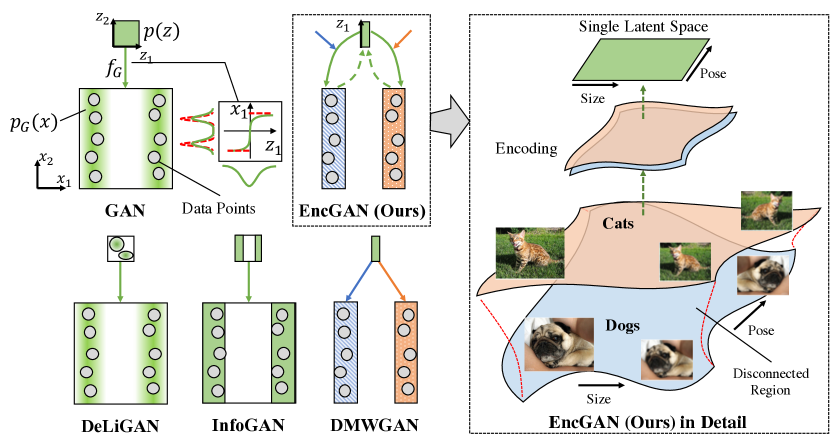
Figure 1: Various GAN models trained on 2-manifold data are shown schematically. Green color indicates shared elements (functions, distributions) whereas blue and red indicate distinct elements. On the right, the encoding process of EncGAN is shown in detail. The encoding combines multiple manifolds into a single latent space by eliminating the disconnected region. From this, the latent space gets to present the common abstract features (size and pose). See Sec. 2.1 for more on others.

2 Difficulties in Learning Multiple Manifolds with GAN

In conventional GANs [6], the generator consists of a latent-space distribution $p(z)$ and a decoding mapping $f_{G}:Z\to X$. Transforming $p(z)$ using $f_{G}$, an input-space distribution $p_{G}(x)$ is defined to model the data, and this particular way of defining $p_{G}(x)$ introduces a manifold structure. The structure further becomes a single, globally connected manifold, when $p(z)$ is set to a uniform or a normal distribution as usual. This is because the supports of aforesaid distributions are globally connected space, and $f_{G}$ is a smooth and injective map. As smooth, injective maps preserve the connectedness before and after the mapping, the manifold produced from $f_{G}$ is the same globally connected space as the latent space [11].

A consequence of this is a difficulty in learning multi-manifold data. As the generator can only present a single connected manifold, the best possible option for the generator is to cover all the manifolds and approximate the disconnected regions with low densities. This requires the generator to learn a highly non-linear $f_{G}$ because the density is obtained, using change of variable, as $p_{G}(x)=p(z)/\sqrt{\det\left(J^{\top}J\right)}$ and the Jacobian $J=(\partial f_{G}/\partial z)$ has to be large to present a low density in $p_{G}(x)$ (see Figure 1). Highly nonlinear functions are hard to learn and often lead to a mode collapse problem [15, 11, 19]. Moreover, even if the generator succeeds in learning all the manifolds, unrealistic data are sometimes generated as the model presents only an approximation to the disconnection [11].

2.1 Separate Manifold Modeling in Extended GANs

Recently, several extended GAN models are suggested to tackle the multi-manifold learning. The models can be categorized into two, according to which component of the generator is extended. The first approach extends a single decoding mapping $f_{G}$ to multiple decoding mappings $\{f_{G}^{(i)}\}_{i=1}^{A}$ [11, 5, 10] (see Figure 1, DMWGAN), from which a disconnected manifold is obtained. In particular, each component distribution $p_{G}^{(i)}$ obtained from $f_{G}^{(i)}$ models an individual manifold. The second approach extends the latent-space itself to a disconnected space, by using Gaussian mixture latent distribution [19, 7] or by employing discrete latent variables [4] (see Figure 1, DeLiGAN and InfoGAN). Here, each mixture component or discrete variable models an individual manifold.

Although these extensions work quite well, they could be inefficient as they consider each manifold separately. Multiple decoding mappings could require a larger number of parameters, and the disconnected latent modeling could require much complexity in $f_{G}$, as each disconnected latent region has to be mapped differently. Also, they can hardly capture the shared structure that multi-manifold data generally involves. As we have seen in the cats and dogs example, the manifolds likely share their structures according to the abstract smooth features. The separate modeling of manifolds cannot consider this structure, so they miss learning the abstract features shared among the manifolds.

3 Encoder-Powered GAN

Our objective is to model multi-manifold data without having difficulties due to the disconnections. Also, we aim to model the data efficiently and capture the abstract features shared among the manifolds. Here, we explain the proposing encoder-powered GAN in detail and how it can meet these objectives. We first focus on a single linear layer then move on to the encoder network inheriting the principles of the linear layer. Among others, the most important contribution we make is the inverted formulation using the bias regularizer. We will see shortly that this enables a tractable model training with mathematical guarantees.

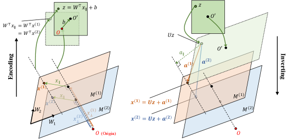
Figure 2: Encoding and Inverting in a linear layer. Encoding: Two points $x^{(1)}$ and $x^{(2)}$ belong to different manifolds but mapped to the same $z$ as they have the same tangential components $x_{\parallel}$ to the column space of $W$. Inverting: A latent point $z$ is transformed by $U=W(W^{\top}W)^{-1}$, then different decoding biases $a^{(1)}$ and $a^{(2)}$ are added to generate $x^{(1)}$ and $x^{(2)}$ for different manifolds. The decoding biases are learned as separated parameters but regularized to have the same tangential components to implicitly define the encoder.

3.1 Linear Encoding Layer

Modeling and Abstracting the Multiple Manifolds

Consider a linear encoding layer with a weight $W\in\mathbb{R}^{d_{x}\times d_{z}}$ ($d_{z}<d_{x}$) and a bias $b\in\mathbb{R}^{d_{z}}$. When an input $x\in\mathbb{R}^{d_{x}}$ is passed through the layer, we know from the basic linear algebra that only the tangential component to the column space of $W$ survives, and the normal component is lost. We use this property to model the multiple manifolds and to extract the shared features among them. In particular, we model the manifolds as spaces parallel to the column space of $W$, where they differ only in the normal component (see Figure 2, left). This means, a point lying on the $i$-th manifold can be described as

$$x^{(i)}=x_{\parallel}+x_{\perp}^{(i)},$$

where the tangential component $x_{\parallel}$ is variable and shared among the manifolds and the normal component $x_{\perp}^{(i)}$ is fixed and distinct for each $i$-th manifold. With this modeling, the latent output

$$z=W^{\top}x_{\parallel}+b$$ (1)

is the same for the points lying on different manifolds as long as they have the same tangential components. This way, the linear layer captures the smooth features shared among the manifolds in its latent output. At the same time, it abstracts multiple manifolds into a single latent space by eliminating the disconnected region along the normal component.

Data Generation

Data is generated by inverting the encoding mapping (Eq. 1), from which a random latent sample $z$ is transformed into an input data sample. Firstly, multiplying the pseudo-inverse of $W$ on the both sides of Eq. 1, we obtain a tangential component as $x_{\parallel}=W(W^{\top}W)^{-1}(z-b)$. Then, we add a normal component $x_{\perp}^{(i)}$ to generate the data sample $x^{(i)}$ for each $i$-th manifold:

$$x^{(i)}=W(W^{\top}W)^{-1}(z-b)+x_{\perp}^{(i)}.$$ (2)

Here, the normal components $\{x_{\perp}^{(i)}\}_{i=1}^{A}$ restore the disconnections between the manifolds. The normal components can be either trained or directly computed from the encoder inputs depending on the model setting. In this work, we only consider the trainable setting.

Inverted Formulation

The primal formulation given above contains the pseudo-inverse of $W$, which is challenging to compute and unstable for a gradient descent learning. Our approach here is to construct a dual formulation based on an inverted, decoder-like parameterization. Although the model mainly learns decoders under this regime, they are properly regularized such that the primal single encoder can be recovered anytime.

Let us start by rearranging the Eq. 2 as

$$x^{(i)} =Uz+a^{(i)},$$

where $U=W(W^{\top}W)^{-1}$ denotes a decoder weight and $a^{(i)}=x_{\perp}^{(i)}-Ub$ denotes a decoder bias for the $i$-th manifold (see Figure 2, right). Comparing this rearrangement with a general decoding mapping, the condition that makes the decoders consistent with the encoder can be inferred: The weight $U$ and the tangential component of the bias $a_{\parallel}^{(i)}=-Ub$ are shared among all the manifolds. If we make the decoders keep this condition while training, we can always recover the encoder by $W=U(U^{\top}U)^{-1}$ and $b=-(U^{\top}U)^{-1}U^{\top}a^{(i)}$. Making $U$ shared is as trivial as setting the same weight for all the manifolds, but making $a_{\parallel}^{(i)}$ shared requires a regularization.

Bias Regularizer

We could make $a_{\parallel}^{(i)}$ shared, by minimizing the sum of the variance of them: $\text{trace}(\text{cov}(a_{\parallel}^{(i)}))$. However, computing this term is intractable due to the inversion $(U^{\top}U)^{-1}$ inside of $a_{\parallel}^{(i)}=U(U^{\top}U)^{-1}U^{\top}a^{(i)}$.

Proposition 1.

The following inequality holds

$$\text{trace}\left(\text{cov}(U^{\top}a^{(i)})\right) \geq\frac{1}{d_{z}}H(\{\lambda_{k}\}_{k=1}^{d_{z}})\text{trace}\left(\text{cov}(a_{\parallel}^{(i)})\right)$$

where $\{\lambda_{k}\}_{k=1}^{d_{z}}$ are the eigenvalues of $U^{\top}U$ and $H(\cdot)$ denotes a harmonic mean.

Proof.

Note that

$$\text{trace}\left(\text{cov}(a_{\parallel}^{(i)})\right) =\text{trace}\left(\text{cov}(U(U^{\top}U)^{-1}U^{\top}a^{(i)})\right)$$

$$=\text{trace}\left(\text{cov}(U^{\top}a^{(i)})(U^{\top}U)^{-1}\right)$$

$$\leq\text{trace}\left(\text{cov}(U^{\top}a^{(i)})\right)\text{trace}\left((U^{\top}U)^{-1}\right),$$

where the second line is obtained from the cyclic property of trace and the last line is obtained from the Cauchy-Schwarz inequality of the positive semi-definite matrices (see Appendix A for the details). ∎

As the harmonic mean in the proposition is constant from the perspective of $a_{\parallel}^{(i)}$, we can minimize the original term by minimizing the upper bound instead. With an additional $\log$ function to match the scale due to the dimensionality, we propose the upper bound as a regularizer for the shared $a_{\parallel}^{(i)}$:

$$R_{bias}=\log\left(\text{trace}\left(\text{cov}(U^{\top}a^{(i)})\right)\right)$$

3.2 Encoder Network

A single linear layer is, of course, insufficient as it can only model the linear manifolds and eliminate the disconnected region only linearly. So we build a deep encoder network to model the complex nonlinear manifolds. In each linear layer of the encoder, the disconnected region is linearly eliminated, so there remains a residual nonlinear region that is not eliminated. The following nonlinear layer flattens this region, thus the next linear layer can eliminate it further up to a smaller number of dimensions. Continuing this procedure layer-by-layer, the encoder finally yields a single low-dimensional linear space shared among the manifolds, in which the disconnected region is fully eliminated.

Instead of directly considering the encoder, we again use the inverted formulation of defining a decoder and regularizing it such that the encoder can be recovered. Specifically, for each of the linear layers in the decoder, we set multiple biases and apply the regularizer proposed above. As the other types of layers (e.g., batch-norm or non-linear activations) can be inverted in a closed form, we can invert the entire decoder to recover the original encoder as needed.

Training

If we denote the decoding weight of the $l$-th linear layer as $U_{l}$ and the decoding biases as $\{a_{l}^{(i)}\}_{i=1}^{A}$ , we can express the ancestral sampling of data as:

$$x \sim f_{G}^{(i)}\left(z;\{U_{l},a_{l}^{(i)}\}_{l=1}^{L}\right)\quad\text{where}\enskip z\sim p(z),\enskip i\sim\pi_{i}.$$

Here, $\pi_{i}$ stands for the probability of selecting the $i$-th bias. This probability could be also learned using the method proposed in [11], but it is beyond our scope and we fix it as $1/A$. Now, denoting the real data distribution as $p_{R}$ and the fake distribution that the above sampling presents as $p_{G}$, we define our GAN losses as:

$$\text{{GAN Loss:} }\begin{cases}\mathcal{L}_{G}=-E_{x\sim p_{G}}\left[D(x)\right]+\lambda\sum_{l=1}^{L}\log\left(\text{trace}\left(\text{cov}(U_{l}^{\top}a_{l}^{(i)})\right)\right)\\ \mathcal{L}_{D}=E_{x\sim p_{G}}\left[D(x)\right]-E_{x\sim p_{R}}\left[D(x)\right]\end{cases}$$

where $\mathcal{L}_{G}$ and $\mathcal{L}_{D}$ are the generator and the discriminator losses respectively and $\lambda$ is a regularization weight. We use Wasserstein GAN (WGAN) [1] so the discriminator $D(x)$ is limited to a $k$-Lipschitz function.

Encoding

With the inverted, decoder-like formulation, we have circumvented the computation of the inversions in data generation; but conversely, we have difficulties in the encoding, especially due to the convolutional layers. A recent work considers this difficulty and prove that a distance minimization approach, $z=\arg\min_{\tilde{z}}\|x-f_{G}(\tilde{z})\|^{2}$, can find the correct latent value $z$ for $x$ [14]. Applying this to our case, we compute the $z$ and the proper decoding biases by:

$$z,\{a_{l}\}_{l=1}^{L}=\arg\min_{\tilde{z},\{\tilde{a}_{l}\}_{l=1}^{L}}\left\|x-f_{G}\left(\tilde{z};\{\tilde{a}_{l}\}_{l=1}^{L}\right)\right\|^{2}+\mu\sum_{l=1}^{L}\log\left(\left\|U_{l}^{\top}a_{l}-U_{l}^{\top}\bar{a}_{l,\parallel}\right\|^{2}\right),$$ (3)

where the second term is introduced to regularize the shared tangential component condition, $\mu$ is the regularization weight, and $\bar{a}_{l,\parallel}$ is the mean of the $\{a_{l,\parallel}^{(i)}\}_{i=1}^{A}$.

4 Experiments

Table 1: FID (smaller is better) and Disentanglement (larger is better) scores are shown. We compare WGAN [1], DMWGAN [11], $\beta$-VAE [9], InfoGAN [4] with our model. The mean and std. values are computed from 10 (MNIST) and 5 (3D-Chair) replicated experiments.

		WGAN	DMWGAN	$\beta$-VAE	InfoGAN	EncGAN (Ours)	EncGAN, $\lambda=0$
FID	MNIST	$10.13\pm 3.16$	$\mathbf{5.41\pm 0.34}$	$58.43\pm 0.23$	$12.17\pm 1.30$	$\mathbf{5.69\pm 0.89}$	$15.74\pm 10.00$
	3D-Chair	$\mathbf{125.32\pm 1.16}$	-	$217.12\pm 0.55$	$187.94\pm 9.51$	$\mathbf{125.27\pm 4.34}$	$128.44\pm 7.06$
Disent.	MNIST (slant)	$1.62\pm 0.41$	-	$\mathbf{5.04\pm 1.19}$	-	$2.15\pm 0.17$	$1.76\pm 0.35$
	MNIST (width)	$1.68\pm 0.49$	-	$\mathbf{5.63\pm 0.75}$	-	$2.93\pm 0.60$	$2.75\pm 0.67$
	3D-Chair (height)	$2.14\pm 0.20$	-	$\mathbf{8.10\pm 0.20}$	-	$3.27\pm 1.73$	$2.76\pm 0.31$
	3D-Chair (bright.)	$3.53\pm 0.80$	-	$3.96\pm 0.20$	-	$\mathbf{4.45\pm 0.66}$	$4.24\pm 0.54$

Datasets

We experiment on MNIST [13], 3D-Chair [2] and UT-Zap50k [20] image datasets. 3D-Chair contains 1393 distinct chairs rendered for 62 different viewing angles (total 86,366 images); in experiments, only front-looking 44,576 images are used and rescaled to 64x64 grayscale images. UT-Zap50k contains images of 4 different types of shoes (total 50,025 images); rescaled to 32x32.

Model Architecture

We use DCGAN [17]-like model architectures for all the datasets (see Appendix B for the complete information). For each of the linear layers in the generator, the number of biases $A$ are set as 10 (MNIST), 20 (3D-Chair) and 4 (UT-Zap50k). Although our multi-biased linear layer can be applied to both fully-connected and transposed-convolution layers, we apply it only to the former. This is sufficient for our purpose since discrete features rarely exist for such small sized kernel patches. In the discriminator, we use a spectral normalization [16] to achieve the $k$-Lipschitz condition for WGAN. For training and encoding, Adam [12] is used with the defaults except for the learning rate, 0.0002.

4.1 Multi-Manifold Learning

Although the true multi-manifold structures of the datasets are unknown, we can make a reasonable guess by considering which features are discrete and which features are smooth. MNIST involves discrete digits and smoothly varying writing styles, so we can guess it has a distinct manifold for each digit and the manifolds present the varying writing styles. Similarly, 3D-Chair would have a distinct manifold for each category of chairs, and the manifolds represent varying viewing angles, shapes or brightness; UT-Zap50k would have a distinct manifold for each type of shoes, and the manifolds represent varying colors or styles.

Looking at Figure 3 row-wise, we can see that our model learns distinct manifolds well, in accordance with our guesses (see in particular the rolling chairs and the boots). Column-wise, we can see that semantic features (e.g., stroke weight) are well aligned among the manifolds, which indicates that our model learns the shared abstract features in the latent space. To quantitatively examine the sample quality, we compute the FID score [8]. FID score is widely used to quantitatively measure the diversity and quality of the generated image samples, which also gives a hint of the presence of a mode collapse. Table 1 shows that our model has better or comparable FID score than others.

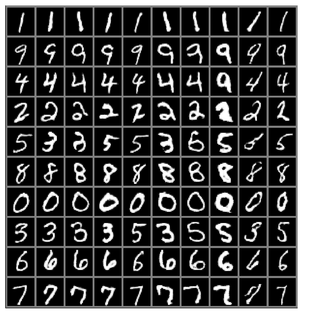
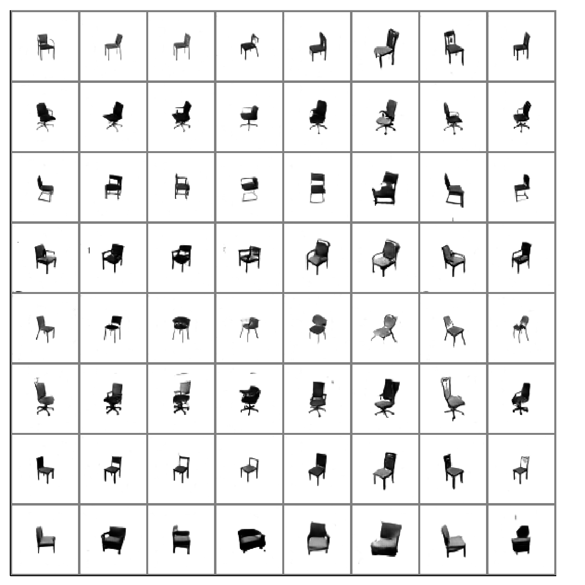
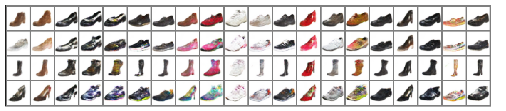
Figure 3: Images generated from the trained EncGANs. In all subfigures, rows indicate distinct manifolds induced by different biases (only 8 out of 20 are shown for 3D-Chair). The latent codes are randomly sampled and shared column-wise. Row-wise It can be seen that each row captures distinct discrete feature, particularly distinct digit (except 4, 9 and 3, 5 share the manifolds), category of chairs (e.g., leg and armrest types) and type of shoes. (e.g., boots and sneakers). Column-wise It can be seen that smooth features are shared among the manifolds, particularly stroke weight, slant (MNIST), viewing angle, height (3D-Chair), and colors (UT-Zap50k).

4.2 Disentangled Abstract Features

To examine how much our learned latent features are disentangled, we define a disentanglement score and compare it with other models. We first take a few images from the dataset and manually change one of the smooth features that corresponds to a known transformation. Then we encode these images to the latent codes, analyze the covariance, and set the ratio of the first eigenvalue to the second as the disentanglement scores (see Appendix C for the details). Table 1 shows our model gets better scores than other models, but sometimes not as good as $\beta$-VAE. But, note that our model is not guided in information theoretic sense to disentangle the features as $\beta$-VAE and InfoGAN, yet still shows good disentanglement as Fig. 4.

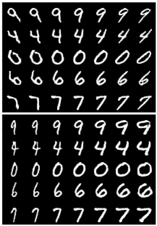
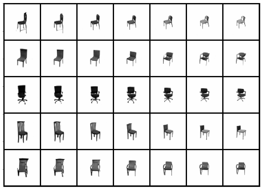
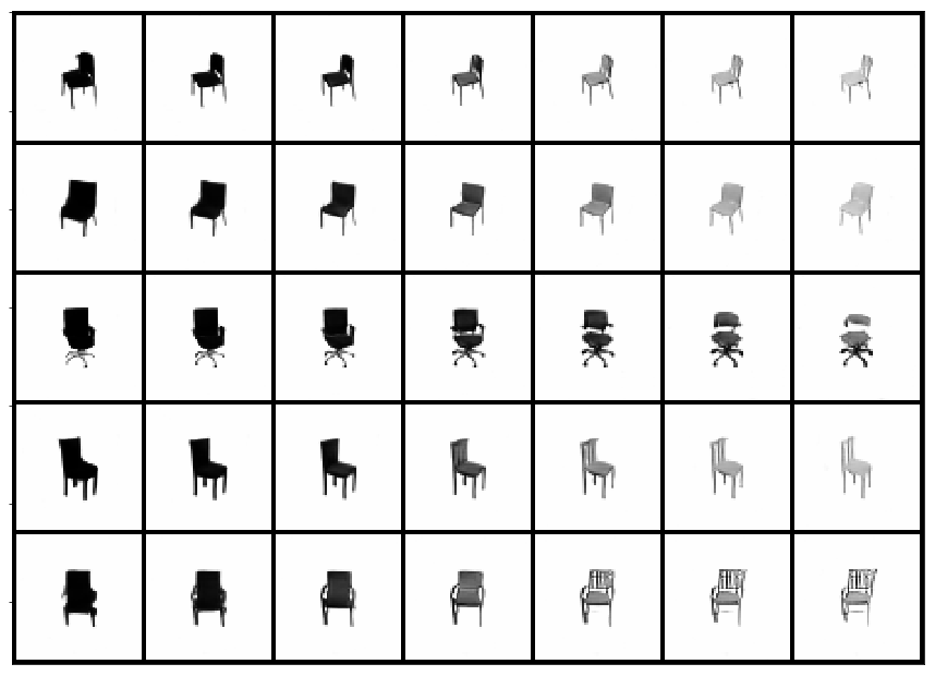
Figure 4: Disentangled features. Images are arranged the same as Fig. 3, except the columns represent linear changes in the latent space along the first eigenvector in the disentanglement score analysis (see Sec. 4.2). Slant, width (MNIST), height and brightness (3D-Chair) components are shown.

4.3 Style Transfer

We demonstrate a style-transfer between images using our model, by matching the latent codes. To make a style-transfer in other models (e.g., $\beta$-VAE), we usually need to separate the discrete and smooth features. Then, we transfer only the smooth features such that the style is transferred, not the identity of the object. In EncGAN, on the other hand, the latent space contains the smooth features only, as the discrete features reside in the biases. Thus, we can make style-transferred images simply by replacing the latent code of the source image with that of the target images, and regenerate the data (see Fig. 5).

Interestingly, EncGAN is even able to style-transfer the images that are off the trained distribution (see the red boxes). This is an exclusive property of EncGAN due to the encoder. If the encoder generalizes well (which apparently does), it can recognize the abstract features of an image even if the image has added frame noises or rectangle noises. Once the features are recognized, the model knows how to transform this image smoothly just like the original data. So the style-transferred images can be obtained with the noises still remained, as the noises are stored in the form of biases (computed from Eq. 3) and restored during the regeneration like discrete features.

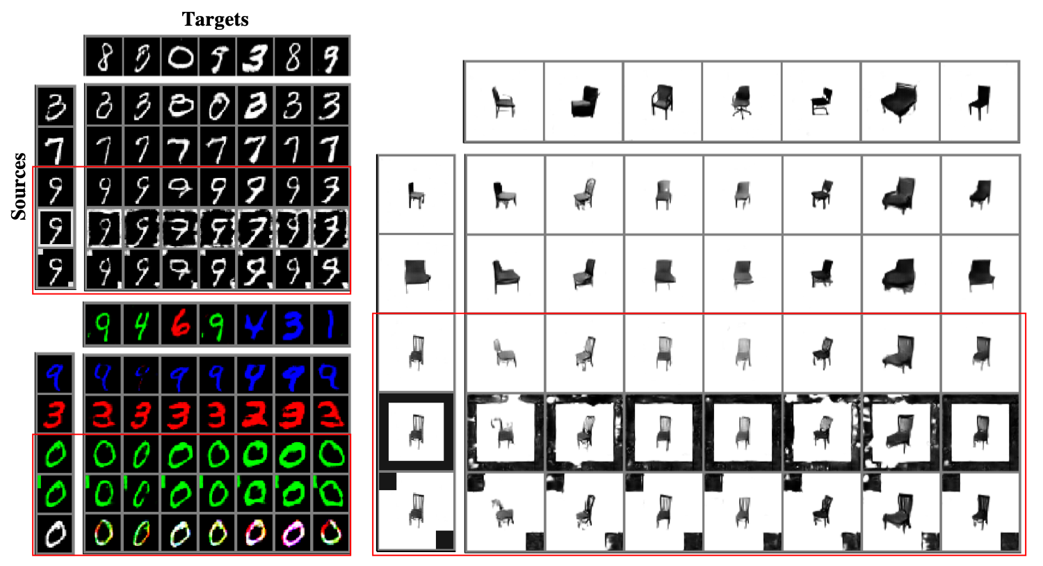
Figure 5: Style transfer results. In each source image set, the last two images are derived from the third image by adding frames, rectangles and changing colors. The derived source images are clearly off the trained distribution, but their style-transfer results are quite good and consistent with the original style-transfer results (highlighted in red boxes). (For this particular experiment, we trained EncGAN on RGB-MNIST, a simple extension to MNIST by coloring with either R, G, or B. We can see that the white image is fairly transferred even though the model never saw the white color.)

5 Conclusion

In this work, we considered the problem of multi-manifold learning by proposing encoder-powered GAN (EncGAN). We showed that EncGAN successfully learns the multi-manifold structure of the data and captures the disentangled features shared among the manifolds. As EncGAN uses an encoder to abstractly model the data, it showed a potential to be generalized to unseen data, as demonstrated in the style-transfer experiment. If it is trained with larger datasets such as ImageNet in the future, we expect EncGAN becomes more versatile that it could be able to infer the manifolds of different datasets (not just the data with noise). Another line of future work would be transfer-learning the encoder from the pre-trained classifier models, which would bring a great boost in GAN training.

Appendix Appendix A Proposition 1 and the Proof

Proposition.

The following inequality holds

$$\text{trace}\left(\text{cov}(U^{\top}a^{(i)})\right) \geq\frac{1}{d_{z}}H(\{\lambda_{k}\}_{k=1}^{d_{z}})\text{trace}\left(\text{cov}(a_{\parallel}^{(i)})\right)$$

where $\{\lambda_{k}\}_{k=1}^{d_{z}}$ are the eigenvalues of $U^{\top}U$ and $H(\cdot)$ denotes a harmonic mean.

Proof.

Note that

$$\text{trace}\left(\text{cov}(a_{\parallel}^{(i)})\right) =\text{trace}\left(\text{cov}(U(U^{\top}U)^{-1}U^{\top}a^{(i)})\right)$$

$$=\text{trace}\left(\frac{1}{A-1}\sum_{i=1}^{A}U(U^{\top}U)^{-1}U^{\top}(a^{(i)}-\bar{a})(a^{(i)}-\bar{a})^{\top}U(U^{\top}U)^{-1}U^{\top}\right)$$

$$=\text{trace}\left(\frac{1}{A-1}\sum_{i=1}^{A}U^{\top}(a^{(i)}-\bar{a})(a^{(i)}-\bar{a})^{\top}U(U^{\top}U)^{-1}\right)$$

$$=\text{trace}\left(\text{cov}(U^{\top}a^{(i)})(U^{\top}U)^{-1}\right)$$

$$\leq\text{trace}\left(\text{cov}(U^{\top}a^{(i)})\right)\text{trace}\left((U^{\top}U)^{-1}\right),$$

where the second and the fourth lines use the definition of the covariance, third line is obtained from the cyclic property of trace and the last line is obtained from the Cauchy-Schwarz inequality of the positive semi-definite matrices. Thus,

$$\text{trace}\left(\text{cov}(U^{\top}a^{(i)})\right) \geq\text{trace}\left(\text{cov}(a_{\parallel}^{(i)})\right)/\text{trace}\left((U^{\top}U)^{-1}\right)$$

$$=\frac{1}{D}H(\{\lambda_{d}\}_{d=1}^{D})\text{trace}\left(\text{Var}(a_{\parallel}^{(i)})\right)$$

where $\{\lambda_{d}\}_{d=1}^{D}$ are eigenvalues of $U^{\top}U$ and $H(\cdot)$ denotes the harmonic mean. ∎

Appendix Appendix B Model Architecture and Experimenting Environments

We used machines with one NVIDIA Titan Xp for the training and the inference of all the models.

Appendix B.1 MNIST

We use $A=10$ distinct decoding biases in the model. In the training, we set the regularization weight $\lambda=0.05$ and use the Adam optimizer with learning rate 0.0002. In the encoding, we use the Adam optimizer with learning rate 0.1, and the set the regularization weight $\mu=0.1$.

Table B.1: EncGAN architecture used for MNIST dataset

Generator	Discriminator
Input(8)	Input(1,28,28)
Full(1024), BN, LReLU(0.2)	Conv(c=64, k=4, s=2, p=1), BN, LReLU(0.2)
Full(6272), BN, LReLU(0.2)	Conv(c=128, k=4, s=2, p=1), BN, LReLU(0.2)
ReshapeTo(128,7,7)	ReshapeTo(6272)
ConvTrs(c=64, k=4, s=2, p=1), BN, LReLU(0.2)	Full(1024), BN, LReLU(0.2)
ConvTrs(c=32, k=4, s=2, p=1), BN, LReLU(0.2)	Full(1)
ConvTrs(c=1, k=3, s=1, p=1), Tanh

Appendix B.1.1 Notes on the Other Compared Models

Overall, we match the architecture of other models with our model for fair comparison. Some differences to note are:

• DMWGAN: We used 10 generators. Each generator has the same architecture as ours except the number of features or the channels are divided by 4, to match the number of trainable parameters. Note that 4 is the suggested number from the original paper.

• $\beta$-VAE: We used Bernoulli likelihood.

• InfoGAN: Latent dimensions consist of 1 discrete variable (10 categories), 2 continuous variable and 8 noise variable.

Appendix B.2 3D-Chair

We use $A=20$ distinct decoding biases in the model. In the training, we set the regularization weight $\lambda=0.05$ and use the Adam optimizer with learning rate 0.0002. In the encoding, we use the Adam optimizer with learning rate 0.1, and the set the regularization weight $\mu=0.1$.

Table B.2: EncGAN architecture used for 3D-Chair dataset.

Generator	Discriminator
Input(10)	Input(1,64,64)
Full(256), BN, LReLU(0.2)	Conv(c=64, k=4, s=2, p=1), BN, LReLU(0.2)
Full(8192), BN, LReLU(0.2)	Conv(c=128, k=4, s=2, p=1), BN, LReLU(0.2)
ReshapeTo(128,8,8)	Conv(c=128, k=4, s=2, p=1), BN, LReLU(0.2)
ConvTrs(c=64, k=4, s=2, p=1), BN, LReLU(0.2)	ReshapeTo(8192)
ConvTrs(c=32, k=4, s=2, p=1), BN, LReLU(0.2)	Full(1024), BN, LReLU(0.2)
ConvTrs(c=16, k=4, s=2, p=1), BN, LReLU(0.2)	Full(1)
ConvTrs(c=1, k=3, s=1, p=1), Tanh

Appendix B.2.1 Notes on the Other Compared Models

• $\beta$-VAE: We used Bernoulli likelihood.

• InfoGAN: Latent dimensions consist of 3 discrete variable (20 categories), 1 continuous variable and 10 noise variable.

Appendix B.3 UT-Zap50k

We use $A=4$ distinct decoding biases in the model. For the regularization weight in the training, we start with $\lambda=5e-6$ then raise to $\lambda=5e-4$ after 300 epochs.

Table B.3: EncGAN architecture used for UT-Zap50k dataset.

Generator	Discriminator
Input(8)	Input(3,32,32)
Full(512), BN, LReLU(0.2)	Conv(c=128, k=4, s=2, p=1), BN, LReLU(0.2)
Full(1024), BN, LReLU(0.2)	Conv(c=256, k=4, s=2, p=1), BN, LReLU(0.2)
Full(8192), BN, LReLU(0.2)	Conv(c=512, k=4, s=2, p=1), BN, LReLU(0.2)
ReshapeTo(512,4,4)	ReshapeTo(8192)
ConvTrs(c=256, k=4, s=2, p=1), BN, LReLU(0.2)	Full(1024), BN, LReLU(0.2)
ConvTrs(c=128, k=4, s=2, p=1), BN, LReLU(0.2)	Full(512), BN, LReLU(0.2)
ConvTrs(c=64, k=4, s=2, p=1), BN, LReLU(0.2)	Full(1)
ConvTrs(c=3, k=3, s=1, p=1), Tanh

Appendix Appendix C Disentanglement Score

To compute the disentanglement score, we first take 500 images from the dataset and manually change one of the smooth features that corresponds to a known transformation. For example, we change the slant of the MNIST digits by taking a sheer transform. With 11 different degrees of the transformation, we obtain 5500 transformed images in total. We encode these images to obtain the corresponding latent codes and subtract the mean for each group of the images (originates from the same image) to align all the latent codes. Then, we conduct Principal Component Analysis (PCA) to obtain the principal direction and the spectrum of variations of the latents codes. If the latent features are well disentangled, the dimensionality of the variation should be close to one. To quantify how much it is close to one, we compute the ratio of the first eigenvalue to the second eigenvalue of the PCA covariance, and set it as the disentanglement score.

Appendix Appendix D Effect of the Bias Regularizer

To examine the effectiveness of our bias regularizer, we visualize the raw values of biases $\{a_{l}^{(i)}\}_{i,l}$ and their (pseudo-)tangential component $\{U_{l}^{\top}a_{l}^{(i)}\}_{i,l}$ (see Fig. D.1, D.2). In all figures, we see that the biases are diverse, but their tangential components are well aligned due to the bias regularizer (left). On the contrary, without the regularizer, the tangential components are not aligned (right).

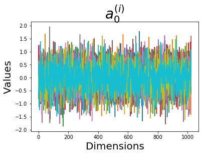
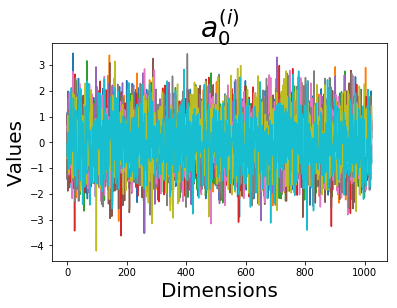
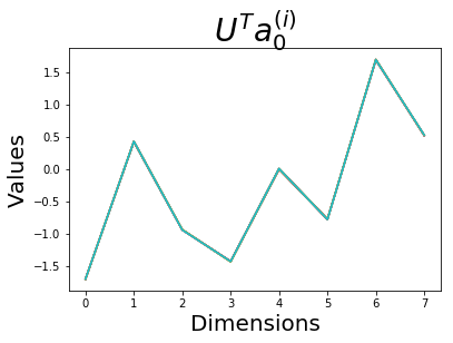
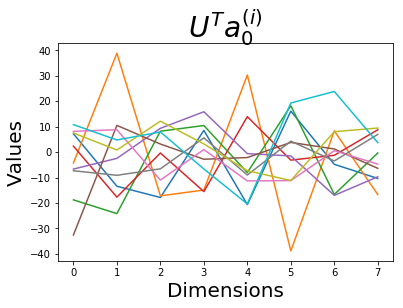
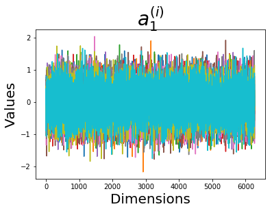
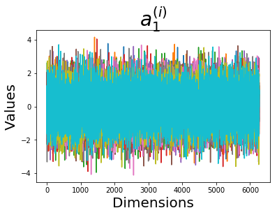
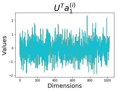
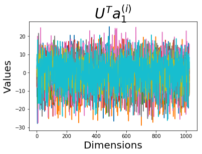
Figure D.1: Biases $a_{l}^{(i)}$ and their (pseudo-)tangential component $U_{l}^{\top}a_{l}^{(i)}$ of the EncGAN models, trained on MNIST. Individual curve indicates each $i$-th bias. Left Parameters of EncGAN Right Parameters of EncGAN without thes regularizer ($\lambda=0$). It can be seen that the regularizer makes the tangential components of the biases well aligned.

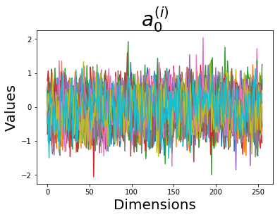
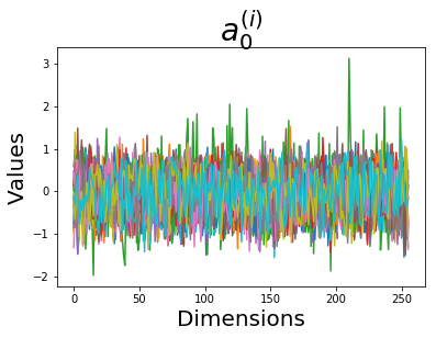
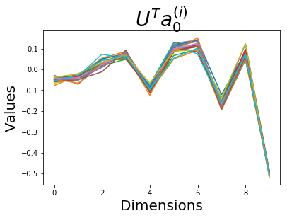
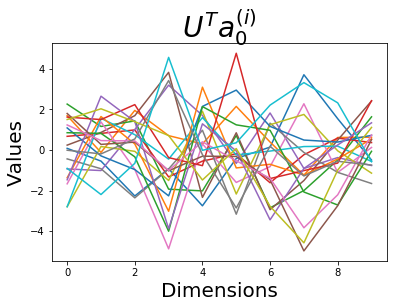
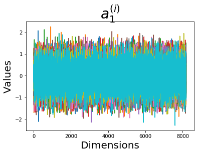
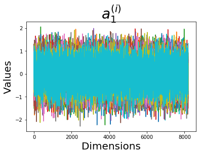
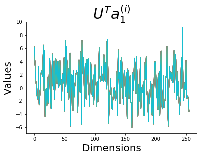
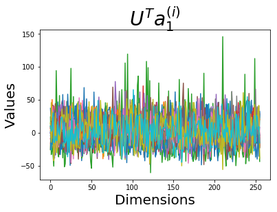
Figure D.2: Biases $a_{l}^{(i)}$ and their (pseudo-)tangential component $U_{l}^{\top}a_{l}^{(i)}$ of the EncGAN models, trained on 3D-Chair. Individual curve indicates each $i$-th bias. Left Parameters of EncGAN Right Parameters of EncGAN without the regularizer ($\lambda=0$). It can be seen that the regularizer makes the tangential components of the biases well aligned.

Appendix Appendix E Samples Generated from Various Models

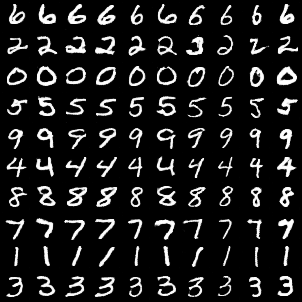
(a) EncGAN

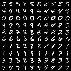
(b) EncGAN ($\lambda=0$)

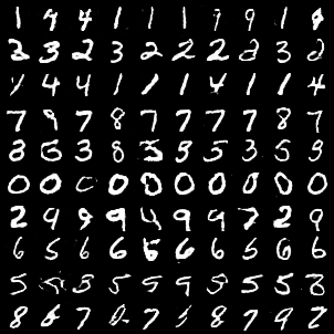
(c) DMWGAN

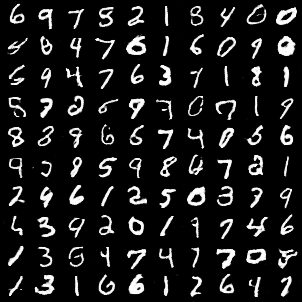
(d) WGAN

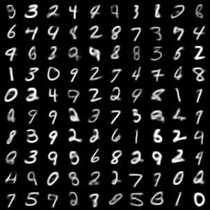
(e) $\beta$-VAE

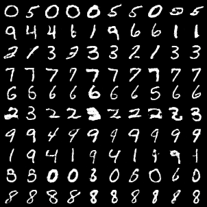
(f) InfoGAN

Figure E.3: MNIST image samples generated from the trained models

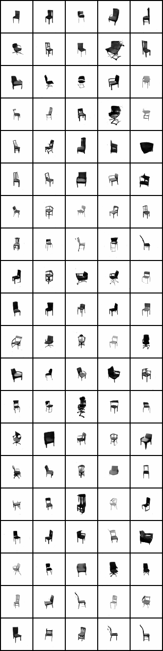
(a) WGAN

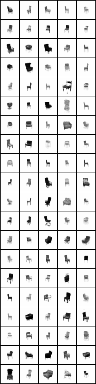
(b) $\beta$-VAE

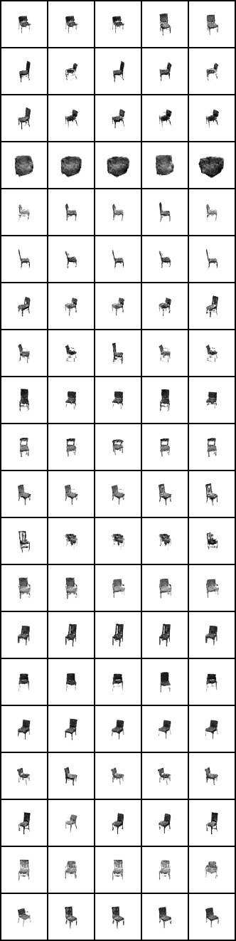
(c) InfoGAN

Figure E.4: 3D-Chair image samples generated from the trained models

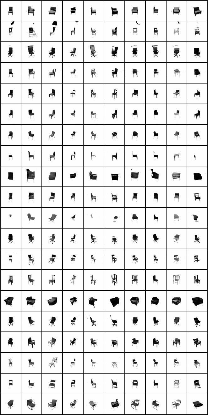
Figure E.5: 3D-Chair image samples generated from the trained EncGAN

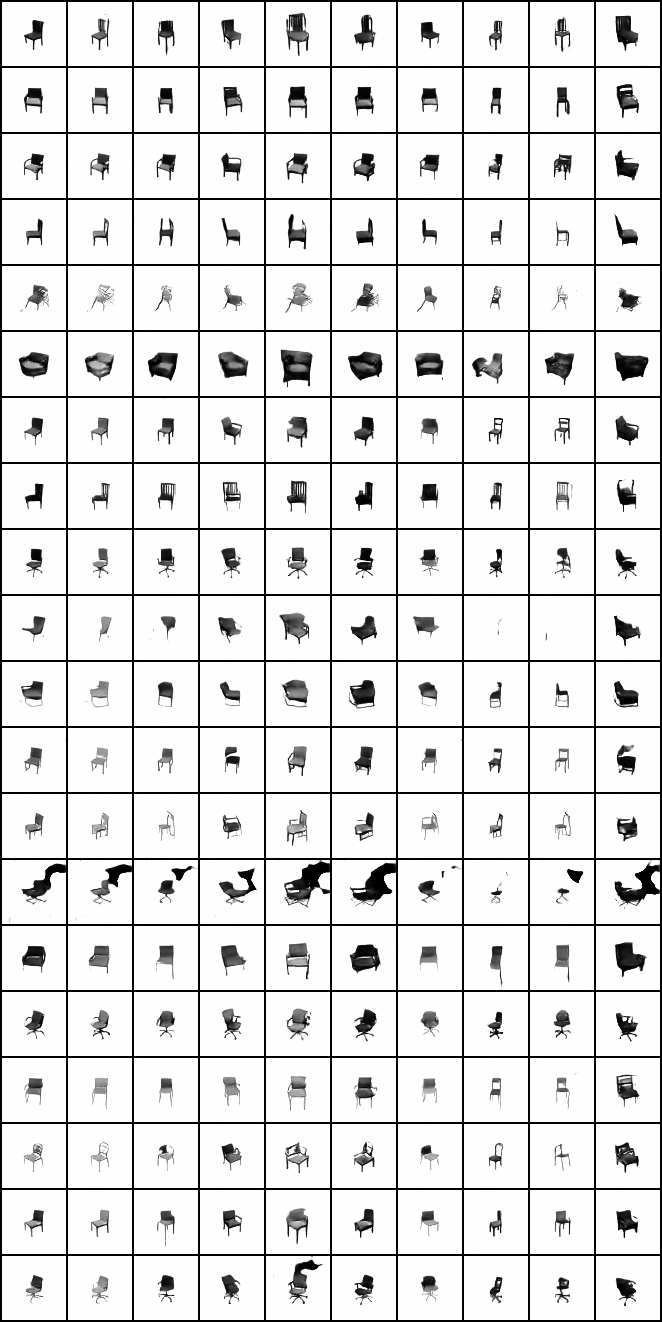
Figure E.6: 3D-Chair image samples generated from EncGAN ($\lambda=0$)

References

- [1] Martin Arjovsky, Soumith Chintala, and Léon Bottou. Wasserstein GAN. January 2017.
- [2] Mathieu Aubry, Daniel Maturana, Alexei A. Efros, Bryan C. Russell, and Josef Sivic. Seeing 3D Chairs: Exemplar Part-Based 2D-3D Alignment Using a Large Dataset of CAD Models. In 2014 IEEE Conference on Computer Vision and Pattern Recognition, pages 3762–3769, Columbus, OH, USA, June 2014. IEEE.
- [3] David Berthelot, Thomas Schumm, and Luke Metz. BEGAN: Boundary Equilibrium Generative Adversarial Networks. arXiv:1703.10717 [cs, stat], March 2017.
- [4] Xi Chen, Yan Duan, Rein Houthooft, John Schulman, Ilya Sutskever, and Pieter Abbeel. InfoGAN: Interpretable Representation Learning by Information Maximizing Generative Adversarial Nets. In D. D. Lee, M. Sugiyama, U. V. Luxburg, I. Guyon, and R. Garnett, editors, Advances in Neural Information Processing Systems 29, pages 2172–2180. Curran Associates, Inc., 2016.
- [5] Arnab Ghosh, Viveka Kulharia, Vinay Namboodiri, Philip H. S. Torr, and Puneet K. Dokania. Multi-Agent Diverse Generative Adversarial Networks. arXiv:1704.02906 [cs, stat], April 2017.
- [6] Ian Goodfellow, Jean Pouget-Abadie, Mehdi Mirza, Bing Xu, David Warde-Farley, Sherjil Ozair, Aaron Courville, and Yoshua Bengio. Generative Adversarial Nets. In Z. Ghahramani, M. Welling, C. Cortes, N. D. Lawrence, and K. Q. Weinberger, editors, Advances in Neural Information Processing Systems 27, pages 2672–2680. Curran Associates, Inc., 2014.
- [7] Swaminathan Gurumurthy, Ravi Kiran Sarvadevabhatla, and R. Venkatesh Babu. DeLiGAN : Generative Adversarial Networks for Diverse and Limited Data. In Proceedings of the IEEE Conference on Computer Vision and Pattern Recognition, pages 166–174, 2017.
- [8] Martin Heusel, Hubert Ramsauer, Thomas Unterthiner, Bernhard Nessler, and Sepp Hochreiter. GANs Trained by a Two Time-Scale Update Rule Converge to a Local Nash Equilibrium. In I. Guyon, U. V. Luxburg, S. Bengio, H. Wallach, R. Fergus, S. Vishwanathan, and R. Garnett, editors, Advances in Neural Information Processing Systems 30, pages 6626–6637. Curran Associates, Inc., 2017.
- [9] Irina Higgins, Loic Matthey, Arka Pal, Christopher Burgess, Xavier Glorot, Matthew Botvinick, Shakir Mohamed, and Alexander Lerchner. Beta-Vae: Learning Basic Visual Concepts with a Constrained Variational Framework. November 2016.
- [10] Quan Hoang, Tu Dinh Nguyen, Trung Le, and Dinh Phung. MGAN: Training Generative Adversarial Nets with Multiple Generators. February 2018.
- [11] Mahyar Khayatkhoei, Maneesh K. Singh, and Ahmed Elgammal. Disconnected Manifold Learning for Generative Adversarial Networks. In S. Bengio, H. Wallach, H. Larochelle, K. Grauman, N. Cesa-Bianchi, and R. Garnett, editors, Advances in Neural Information Processing Systems 31, pages 7343–7353. Curran Associates, Inc., 2018.
- [12] Diederik P. Kingma and Jimmy Ba. Adam: A Method for Stochastic Optimization. December 2014.
- [13] Yann Lecun, Léon Bottou, Yoshua Bengio, and Patrick Haffner. Gradient-based learning applied to document recognition. In Proceedings of the IEEE, pages 2278–2324, 1998.
- [14] Fangchang Ma, Ulas Ayaz, and Sertac Karaman. Invertibility of Convolutional Generative Networks from Partial Measurements. In S. Bengio, H. Wallach, H. Larochelle, K. Grauman, N. Cesa-Bianchi, and R. Garnett, editors, Advances in Neural Information Processing Systems 31, pages 9628–9637. Curran Associates, Inc., 2018.
- [15] Luke Metz, Ben Poole, David Pfau, and Jascha Sohl-Dickstein. Unrolled Generative Adversarial Networks. arXiv:1611.02163 [cs, stat], November 2016.
- [16] Takeru Miyato, Toshiki Kataoka, Masanori Koyama, and Yuichi Yoshida. Spectral Normalization for Generative Adversarial Networks. arXiv:1802.05957 [cs, stat], February 2018.
- [17] Alec Radford, Luke Metz, and Soumith Chintala. Unsupervised Representation Learning with Deep Convolutional Generative Adversarial Networks. November 2015.
- [18] Hang Shao, Abhishek Kumar, and P. Thomas Fletcher. The Riemannian Geometry of Deep Generative Models. arXiv:1711.08014 [cs, stat], November 2017.
- [19] Chang Xiao, Peilin Zhong, and Changxi Zheng. BourGAN: Generative Networks with Metric Embeddings. In S. Bengio, H. Wallach, H. Larochelle, K. Grauman, N. Cesa-Bianchi, and R. Garnett, editors, Advances in Neural Information Processing Systems 31, pages 2269–2280. Curran Associates, Inc., 2018.
- [20] Aron Yu and Kristen Grauman. Fine-Grained Visual Comparisons with Local Learning. In 2014 IEEE Conference on Computer Vision and Pattern Recognition, pages 192–199, Columbus, OH, USA, June 2014. IEEE.