An adaptive finite element method for the sparse optimal control of fractional diffusion

Abstract

We propose and analyze an a posteriori error estimator for a PDE–constrained optimization problem involving a nondifferentiable cost functional, fractional diffusion, and control–constraints. We realize fractional diffusion as the Dirichlet-to-Neumann map for a nonuniformly PDE and propose an equivalent optimal control problem with a local state equation. For such an equivalent problem, we design an a posteriori error estimator which can be defined as the sum of four contributions: two contributions related to the approximation of the state and adjoint equations and two contributions that account for the discretization of the control variable and its associated subgradient. The contributions related to the discretization of the state and adjoint equations rely on anisotropic error estimators in weighted Sobolev spaces. We prove that the proposed a posteriori error estimator is locally efficient and, under suitable assumptions, reliable. We design an adaptive scheme that yields, for the examples that we perform, optimal experimental rates of convergence.

1 Introduction

The main goal of this work is the design and study of a posteriori error estimates for an optimal control problem that entails the minimization of a nondifferentiable cost functional, a state equation that involves the spectral fractional powers of the Dirichlet Laplace operator, and constraints on the control variable. To be precise, let $\Omega\subset\mathbb{R}^{n}$ ($n\geq 1$) be an open and bounded polytopal domain with Lipschitz boundary $\partial\Omega$, $s\in(0,1)$, and $\mathsf{u}_{d}:\Omega\rightarrow\mathbb{R}$ be a desired state. For parameters $\sigma>0$ and $\nu>0$, we define the nonsmooth cost functional

$$J(\mathsf{u},\mathsf{z}):=\frac{1}{2}\|\mathsf{u}-\mathsf{u}_{d}\|^{2}_{L^{2}(\Omega)}+\frac{\sigma}{2}\|\mathsf{z}\|^{2}_{L^{2}(\Omega)}+\nu\|\mathsf{z}\|_{L^{1}(\Omega)}.$$ (1.1)

We will be interested in the numerical approximation of the following nondifferentiable PDE–constrained optimization problem: Find

$$\text{min }J(\mathsf{u},\mathsf{z}),$$ (1.2)

subject to the nonlocal state equation

$$(-\Delta)^{s}\mathsf{u}=\mathsf{z}\text{ in }\Omega,$$ (1.3)

and the control constraints

$$\mathsf{a}\leq\mathsf{z}(x^{\prime})\leq\mathsf{b}\quad\textrm{a.e.~{}~{}}x^{\prime}\in\Omega.$$ (1.4)

For $s\in(0,1)$, the operator $(-\Delta)^{s}$ denotes the spectral fractional powers of the Dirichlet Laplace operator; the so–called spectral fractional Laplacian. We must immediately comment that this definition and the classical one that is based on a pointwise integral formula [40, 57, 59] do not coincide; their difference is positive and positivity preserving [46]. In addition, we also comment that, since we are interested in the nonsmooth scenario, we will assume, in (1.4), that the control bounds $\mathsf{a},\mathsf{b}\in\mathbb{R}$ satisfy that $\mathsf{a}<0<\mathsf{b}$. We refer the reader to [18, Remark 2.1] for a discussion.

The efficient approximation of problems involving the spectral fractional Laplacian carries two essential difficulties. The first, and most important, is that $(-\Delta)^{s}$ is a nonlocal operator [12, 13, 16]. The second feature is the lack of boundary regularity [15], which leads to reduced convergence rates [8, 47]. In fact, as [15, Theorem 1.3] shows, if $\partial\Omega$ is sufficiently smooth, then the solution $\mathsf{u}$ to problem (1.3) behaves like

$$\mathsf{u}(x^{\prime}) \approx\textrm{dist}(x^{\prime},\partial\Omega)^{2s}+\mathsf{v}(x^{\prime}),\quad s\in(0,\tfrac{1}{2}),$$ (1.5)

$$\mathsf{u}(x^{\prime}) \approx\textrm{dist}(x^{\prime},\partial\Omega)+\mathsf{v}(x^{\prime}),\quad s\in(\tfrac{1}{2},1),$$

where $\textrm{dist}(x^{\prime},\partial\Omega)$ denotes the distance from $x^{\prime}$ to $\partial\Omega$ and $\mathsf{v}$ is a smooth function. The case $s=\tfrac{1}{2}$ is exceptional:

$$\mathsf{u}(x^{\prime})\approx\textrm{dist}(x^{\prime},\partial\Omega)|\log(\textrm{dist}(x^{\prime},\partial\Omega))|+\mathsf{v}(x^{\prime}),$$ (1.6)

where $\mathsf{v}$ is, again, a smooth function; see [26] for $\Omega\subset\mathbb{R}^{2}$ and $\partial\Omega$ smooth.

The aforementioned nonlocality difficulty can be overcame with the localization results by Caffarelli and Silvestre [13]. When $\Omega=\mathbb{R}^{n}$, the authors of [13] proved that any power of the fractional Laplacian can be realized as the Dirichlet-to-Neumann map for an extension problem posed in the upper half–space $\mathbb{R}^{n+1}_{+}$. A similar extension property is valid for the spectral fractional Laplacian in a bounded domain $\Omega$ [12, 16]. The latter extension involves a local but nonuniformly elliptic PDE formulated in the semi–infinite cylinder $\mathcal{C}=\Omega\times(0,\infty)$:

$$\textrm{div}\left(y^{\alpha}\nabla\mathscr{U}\right)=0\text{ in }\mathcal{C},\quad\mathscr{U}=0\text{ on }\partial_{L}\mathcal{C},\quad\partial_{\nu^{\alpha}}\mathscr{U}=d_{s}\mathsf{z}\text{ on }\Omega\times\{0\},$$ (1.7)

where $\partial_{L}\mathcal{C}=\partial\Omega\times[0,\infty)$ corresponds to the lateral boundary of $\mathcal{C}$ and $d_{s}=2^{\alpha}\Gamma(1-s)/\Gamma(s)$. The parameter $\alpha$ is defined as $\alpha=1-2s\in(-1,1)$ and the conormal exterior derivative of $\mathscr{U}$ at $\Omega\times\{0\}$ is

$$\partial_{\nu^{\alpha}}\mathscr{U}=-\lim_{y\rightarrow 0^{+}}y^{\alpha}\mathscr{U}_{y};$$ (1.8)

the limit is understood in the distributional sense. We shall refer to $y$ as the extended variable and to the dimension $n+1$, in $\mathbb{R}_{+}^{n+1}$, the extended dimension of problem (1.7). With the extension $\mathscr{U}$ at hand, we thus introduce the fundamental result by Caffarelli and Silvestre [12, 13, 16]: the Dirichlet-to-Neumann map of problem (1.7) and the spectral fractional Laplacian are related by $d_{s}(-\Delta)^{s}\mathsf{u}=\partial_{\nu^{\alpha}}\mathscr{U}\textrm{ in }\Omega.$

The use of the extension problem (1.7) for the discretization of the spectral fractional Laplacian was first used in [47]. The main advantage of the scheme proposed in [47] is that it involves the resolution of the local problem (1.7) and thus its implementation uses basic ingredients of finite element analysis; its analysis, however, involves asymptotic estimates of Bessel functions [1], to derive regularity estimates in weighted Sobolev spaces, elements of harmonic analysis [29, 45], and an anisotropic polynomial interpolation theory in weighted Sobolev spaces [30, 48]. Such an interpolation theory allows for tensor product elements that exhibit an anisotropic feature in the extended dimension, that is in turn needed to compensate the singular behavior of the solution $\mathscr{U}$ in the extended variable $y$ [47, Theorem 2.7], [8, Theorem 4.7].

PDE–constrained optimization problems for fractional diffusion have been considered in a number of works [5, 6, 27, 34, 51]. Recently, the authors of [52] have provided an a priori error analysis for the sparse optimal control problem (1.2)–(1.4). This was mainly motivated by the following considerations:

1. Practitioners claim that the fractional Laplacian seems to better describe many processes. A rather incomplete list of problems where fractional diffusion appears includes finance [41, 53], turbulent flow [22], quasi–geostrophic flows models [14], models of anomalous thermoviscous behaviors [23], biophysics [11], nonlocal electrostatics [38], image processing [33], peridynamics [28, 56], and many others. It is then only natural that interest in efficient approximation schemes for these problems arises and that one might be interested in their control.

2. The cost functional $J$ involves an $L^{1}(\Omega)$–control cost term that leads to sparsely supported optimal controls [18, 58, 63]; a desirable feature, for instance, in the optimal placement of discrete actuators [58].

In [52], the authors first consider an equivalent optimal control problem that involves the local elliptic PDE (1.7) as state equation. Second, since (1.7) is posed on the semi–infinite cylinder $\mathcal{C}=\Omega\times(0,\infty)$, they propose a truncated optimal control problem on $\mathcal{C}_{\mathpzc{Y}}=\Omega\times(0,\mathpzc{Y})$ and derive an exponential error estimate with respect to the truncation parameter $\mathpzc{Y}$. Then, they propose a scheme to approximate the truncated optimal control problem: the first–degree finite element approximation of [47] for the state and adjoint equations and piecewise constant approximation for the optimal control variable. The derived a priori error estimate reads as follows: Given $\mathsf{u}_{d}\in\mathbb{H}^{1-s}(\Omega)$ and $\mathsf{a},\mathsf{b}\in\mathbb{R}$ such that $\mathsf{a}<0<\mathsf{b}$, if $\Omega$ is convex, then

$$\|\bar{\mathsf{z}}-\bar{Z}\|_{L^{2}(\Omega)}\lesssim|\log N|^{2s}N^{-\frac{1}{n+1}},$$ (1.9)

where $\bar{Z}$ corresponds to the optimal control variable of the scheme of [52, Section 6] and $N$ denotes the total number of degrees of freedom of the underlying mesh. The adaptive finite element method (AFEM) that we propose in our work is thus motivated, in addition to the search of a numerical scheme that efficiently solves (1.2)–(1.4) with relatively modest computational resources, by the following considerations:

1. The a priori error estimate (1.9) requires the convexity of the domain $\Omega$ and compatibility conditions on the desired state $\mathsf{u}_{d}$ that are expressed as $\mathsf{u}_{d}\in\mathbb{H}^{1-s}(\Omega)$: it is required that $\mathsf{u}_{d}$ vanishes on $\partial\Omega$ for $s\in(0,\frac{1}{2}]$. If these conditions do not hold then, the a priori error estimate (1.9) is not longer valid. In particular, the violation of the latter condition implies that the adjoint state $\bar{\mathsf{p}}$ will behave as (1.5)–(1.6). On the other hand, if the first condition (the convexity of the domain) is violated, then both the state and adjoint state variables may exhibit singularities in the direction of the $x^{\prime}$ variables. An efficient technique to solve (1.2)–(1.4) must thus resolve both of the aforementioned approximation issues.

2. The sparsity term $\|\mathsf{u}\|_{L^{1}(\Omega)}$, in the cost functional (1.2), yield an optimal control that is non–zero only in sets of small support in $\Omega$ [18, 58, 63]. It is then natural, to efficiently resolve such a behavior, the consideration of AFEMs.

We organize our exposition as follows: In Section 2 we recall the definition of the spectral fractional Laplacian, present the fundamental result by Caffarelli and Silvestre [13], and recall elements from convex analysis. In Section 3 we recall the numerical scheme proposed in [52] and review its a priori error analysis. Section 4, that is a highlight of our contribution, is dedicated to the design and analysis of an ideal a posteriori error estimator for (1.2)–(1.4) that is equivalent to the error. Since, the aforementioned estimator is not computable, we propose, in Section 5 a computable one and show that is equivalent, under suitable assumptions, to the error up to oscillation terms. Finally, in Section 6 we design an AFEM, comment on some implementation details pertinent to the problem, and present numerical experiments that yield optimal experimental rates of convergence.

2 Notation and preliminaries

We adopt the notation of [47, 50]. Besides the semi–infinite cylinder $\mathcal{C}=\Omega\times(0,\infty)$, we introduce, for $\mathpzc{Y}>0$, the truncated cylinder $\mathcal{C}_{\mathpzc{Y}}=\Omega\times(0,\mathpzc{Y})$ and its lateral boundary $\partial_{L}\mathcal{C}{Y}=\partial\Omega\times(0,\mathpzc{Y})$.

For $x\in\mathbb{R}_{+}^{n+1}$, we write $x=(x^{\prime},y)$ with $x^{\prime}\in\mathbb{R}^{n}$ and $y\in(0,\infty)$.

The parameter $\alpha\in(-1,1)$ and the power $s$ of the spectral fractional Laplacian $(-\Delta)^{s}$ are related by the formula $\alpha=1-2s$.

The relation $a\lesssim b$ indicates that $a\leq Cb$, with a constant $C$ which is independent of $a$ and $b$ and the size of the elements in the mesh. The value of the constant $C$ might change at each occurrence.

2.1 The fractional Laplace operator

Since $-\Delta:\mathcal{D}(-\Delta)\subset L^{2}(\Omega)\rightarrow L^{2}(\Omega)$ is an unbounded, positive, and closed operator with dense domain $\mathcal{D}(-\Delta)=H^{2}(\Omega)\cap H_{0}^{1}(\Omega)$ and its inverse is compact, the eigenvalue problem:

$$(\lambda,\varphi)\in\mathbb{R}\times H_{0}^{1}(\Omega)\setminus\{0\}:\quad(\nabla\varphi,\nabla v)_{L^{2}(\Omega)}=\lambda(\varphi,v)_{L^{2}(\Omega)}\quad\forall v\in H_{0}^{1}(\Omega)$$

has a countable collection of eigenpairs $\{\lambda_{k},\varphi_{k}\}_{k\in\mathbb{N}}\subset\mathbb{R}^{+}\times H_{0}^{1}(\Omega)$, with real eigenvalues enumerated in increasing order, counting multiplicities. In addition, $\{\varphi_{k}\}_{k\in\mathbb{N}}$ is an orthogonal basis of $H_{0}^{1}(\Omega)$ and an orthonormal basis of $L^{2}(\Omega)$ [9]. With these eigenpairs at hand, we define, for $s\geq 0$, the fractional Sobolev space

$$\mathbb{H}^{s}(\Omega)=\left\{w=\sum_{k=1}^{\infty}w_{k}\varphi_{k}:\|w\|_{\mathbb{H}^{s}(\Omega)}^{2}=\sum_{k=1}^{\infty}\lambda_{k}^{s}w_{k}^{2}<\infty\right\},$$

where, for $k\in\mathbb{N}$, $w_{k}=(w,\varphi_{k})_{L^{2}(\Omega)}$. We denote by $\mathbb{H}^{-s}(\Omega)$ the dual space of $\mathbb{H}^{s}(\Omega)$. The duality pairing between $\mathbb{H}^{s}(\Omega)$ and $\mathbb{H}^{-s}(\Omega)$ will be denoted by $\langle\cdot,\cdot\rangle$.

We define, for $s\in(0,1)$, the spectral fractional Laplacian $(-\Delta)^{s}$ as

$$(-\Delta)^{s}:\mathbb{H}^{s}(\Omega)\rightarrow\mathbb{H}^{-s}(\Omega),\quad(-\Delta)^{s}w:=\sum_{k=1}^{\infty}\lambda_{k}^{s}w_{k}\varphi_{k},\quad w_{k}=(w,\varphi_{k})_{L^{2}(\Omega)},\quad k\in\mathbb{N}.$$

2.2 An extension property

The operator in (1.7) is in divergence form and thus amenable to variational techniques. However, since the weight $y^{\alpha}$ either blows up, for $-1<\alpha<0$, or degenerates, for $0<\alpha<1$, as $y\downarrow 0$, such a local operator is nonuniformly elliptic; the case $\alpha=0$ is exceptional and corresponds to the regular harmonic extension [12]. This entails dealing with Lebesgue and Sobolev spaces with the weight $y^{\alpha}$ for $\alpha\in(-1,1)$ [13, 16].

Let $D\subset\mathbb{R}^{n+1}$ be open. We define $L^{2}(|y|^{\alpha},D)$ as the Lebesgue space for the measure $|y|^{\alpha}\,\mbox{\rm d}x$. We also define the weighted Sobolev space $H^{1}(|y|^{\alpha},D):=\{w\in L^{2}(|y|^{\alpha},D):|\nabla w|\in L^{2}(|y|^{\alpha},D)\},$ and the norm

$$\|w\|_{H^{1}(|y|^{\alpha},D)}=\left(\|w\|^{2}_{L^{2}(|y|^{\alpha},D)}+\|\nabla w\|^{2}_{L^{2}(|y|^{\alpha},D)}\right)^{\frac{1}{2}}.$$ (2.1)

Since $\alpha=1-2s\in(-1,1)$, $|y|^{\alpha}$ belongs to Muckenhoupt class $A_{2}(\mathbb{R}^{n+1})$ [29, 32, 35, 45, 61]. This, in particular, implies that $H^{1}(|y|^{\alpha},D)$ is Hilbert and that $C^{\infty}(D)\cap H^{1}(|y|^{\alpha},D)$ is dense in $H^{1}(|y|^{\alpha},D)$ (cf. [61, Proposition 2.1.2, Corollary 2.1.6] and [35, Theorem 1]).

To seek for a weak solution to problem (1.7), we introduce the weighted space

$$\mbox{ \raisebox{7.0pt}{\tiny$\circ$} \kern-10.8pt}{H_{L}^{1}}(y^{\alpha},\mathcal{C}):=\left\{w\in H^{1}(y^{\alpha},\mathcal{C}):w=0\textrm{ on }\partial_{L}\mathcal{C}\right\},$$

and notice that the following weighted Poincaré inequality holds [47, ineq. (2.21)]:

$$\|w\|_{L^{2}(y^{\alpha},\mathcal{C})}\lesssim\|\nabla w\|_{L^{2}(y^{\alpha},\mathcal{C})}\quad\forall w\in\mbox{ \raisebox{7.0pt}{\tiny$\circ$} \kern-10.8pt}{H_{L}^{1}}(y^{\alpha},\mathcal{C}).$$

This implies that the seminorm on $\mbox{ \raisebox{7.0pt}{\tiny$\circ$} \kern-10.8pt}{H_{L}^{1}}(y^{\alpha},\mathcal{C})$ is equivalent to (2.1). For $w\in H^{1}(y^{\alpha},\mathcal{C})$, $\operatorname*{tr_{\Omega}}w$ denotes its trace onto $\Omega\times\{0\}$. We recall ([47, Prop. 2.5] and [16, Prop. 2.1])

$$\operatorname*{tr_{\Omega}}\mbox{ \raisebox{7.0pt}{\tiny$\circ$} \kern-10.8pt}{H_{L}^{1}}(y^{\alpha},\mathcal{C})=\mathbb{H}^{s}(\Omega),\qquad\|\operatorname*{tr_{\Omega}}w\|_{\mathbb{H}^{s}(\Omega)}\leq C_{\operatorname*{tr_{\Omega}}}\|w\|_{{\mbox{\,\raisebox{5.1pt}{\tiny$\circ$} \kern-9.1pt}{H}^{1}_{L}}(y^{\alpha},\mathcal{C})},\quad C_{\operatorname*{tr_{\Omega}}}>0.$$ (2.2)

We mention that $C_{\operatorname*{tr_{\Omega}}}\leq d_{s}^{-\frac{1}{2}}$ with $d_{s}=2^{\alpha}\Gamma(1-s)/\Gamma(s)$ [21, Section 2.3]. This property will be of importance in the a posteriori error analysis that we will perform.

Define the bilinear form

$$a:\mbox{ \raisebox{7.0pt}{\tiny$\circ$} \kern-10.8pt}{H_{L}^{1}}(y^{\alpha},\mathcal{C})\times\mbox{ \raisebox{7.0pt}{\tiny$\circ$} \kern-10.8pt}{H_{L}^{1}}(y^{\alpha},\mathcal{C})\rightarrow\mathbb{R},\quad a(w,\phi):=\frac{1}{d_{s}}\int_{\mathcal{C}}y^{\alpha}\nabla w\cdot\nabla\phi\,\mbox{\rm d}x.$$ (2.3)

The weak formulation of problem (1.7) thus reads: Find $\mathscr{U}\in\mbox{ \raisebox{7.0pt}{\tiny$\circ$} \kern-10.8pt}{H_{L}^{1}}(y^{\alpha},\mathcal{C})$ such that

$$a(\mathscr{U},\phi)=\langle\mathsf{z},\phi\rangle\quad\forall\phi\in\mbox{ \raisebox{7.0pt}{\tiny$\circ$} \kern-10.8pt}{H_{L}^{1}}(y^{\alpha},\mathcal{C}).$$ (2.4)

We conclude this section with the fundamental result by Caffarelli and Silvestre [12, 13, 16]: Let $\mathsf{u}$ solve (1.3). If $\mathscr{U}\in\mbox{ \raisebox{7.0pt}{\tiny$\circ$} \kern-10.8pt}{H_{L}^{1}}(y^{\alpha},\mathcal{C})$ solves (2.4), then $\mathsf{u}=\operatorname*{tr_{\Omega}}\mathscr{U}$ and

$$d_{s}(-\Delta)^{s}\mathsf{u}=\partial_{\nu^{\alpha}}\mathscr{U}\textrm{ in }\Omega.$$

2.3 Convex functions and subdifferentials

Let $S$ be a real and normed vector space. Let $\chi:S\rightarrow\mathbb{R}\cup\{\infty\}$ be a convex and proper function and let $v\in S$ be such that $\chi(v)<\infty$. A subgradient of $\chi$ at $v$ is an element $v^{\star}\in S^{\star}$ that satisfies

$$\langle v^{\star},w-v\rangle_{S^{\star},S}\leq\chi(w)-\chi(v)\quad\forall w\in S,$$ (2.5)

where $\langle\cdot,\cdot\rangle_{S^{\star},S}$ denotes the duality pairing between $S^{\star}$ and $S$. We denote by $\partial\chi(v)$ the set of all subgradients of $\chi$ at $v$: the so–called subdifferential of $\chi$ at $v$. Since $\chi$ is convex, $\partial\chi(v)\neq\emptyset$ for all points $v$ in the interior of the effective domain of $\chi$. We conclude with the following property: the subdifferential is monotone, i.e.,

$$\langle v^{\star}-w^{\star},v-w\rangle_{S^{\star},S}\geq 0\quad\forall v^{\star}\in\partial\chi(v),\ \forall w^{\star}\in\partial\chi(w).$$ (2.6)

The reader is referred to [25, 54] for a detailed treatment on convex analysis.

3 A priori error estimates

In this section we briefly review the a priori error analysis for the fully discrete approximation of the optimal control problem (1.2)–(1.4) proposed and investigated in [52]. We also make clear the limitations of such a priori error analysis, thereby justifying the quest for an a posteriori error analysis.

3.1 The extended optimal control problem

We will consider a solution technique for (1.2)–(1.4) that relies on the discretization of an equivalent problem: the extended optimal control problem, which has as a main advantage its local nature. To present it, we first define the set of admissible controls:

$$\mathsf{Z}_{\textrm{ad}}=\{\mathsf{w}\in L^{2}(\Omega):\mathsf{a}\leq\mathsf{w}(x^{\prime})\leq\mathsf{b}\textrm{~{}~{}a.e~{}~{}}x^{\prime}\in\Omega\},$$ (3.1)

where $\mathsf{a}$ and $\mathsf{b}$ are real and satisfy the property $\mathsf{a}<0<\mathsf{b}$; see[18, Remark 2.1]. The extended optimal control problem reads as follows: Find

$$\text{min}\{J(\operatorname*{tr_{\Omega}}\mathscr{U},\mathsf{z}):\mathscr{U}\in\mbox{ \raisebox{7.0pt}{\tiny$\circ$} \kern-10.8pt}{H_{L}^{1}}(y^{\alpha},\mathcal{C}),\mathsf{z}\in\mathsf{Z}_{\textrm{ad}}\}$$ (3.2)

subject to the linear and nonuniformly elliptic state equation

$$a(\mathscr{U},\phi)=\langle\mathsf{z},\operatorname*{tr_{\Omega}}\phi\rangle\quad\forall\phi\in\mbox{ \raisebox{7.0pt}{\tiny$\circ$} \kern-10.8pt}{H_{L}^{1}}(y^{\alpha},\mathcal{C}).$$ (3.3)

We recall that $J$ is defined as in (1.2), with $\sigma,\nu>0$ and $\mathsf{u}_{d}\in L^{2}(\Omega)$. This problem admits a unique optimal pair $(\bar{\mathscr{U}},\bar{\mathsf{z}})\in\mbox{ \raisebox{7.0pt}{\tiny$\circ$} \kern-10.8pt}{H_{L}^{1}}(y^{\alpha},\mathcal{C})\times\mathsf{Z}_{\textrm{ad}}$. More importantly, it is equivalent to the optimal control problem (1.2)–(1.4): $\operatorname*{tr_{\Omega}}\bar{\mathscr{U}}=\bar{\mathsf{u}}$.

3.2 The truncated optimal control problem

The extended optimal control problem involves the state equation (3.3), which is posed on $\mathcal{C}=\Omega\times(0,\infty)$. Consequently, it cannot be directly approximated with standard finite element techniques. However, in view of the exponential decayment of the optimal state in the extended variable [47, Proposition 3.1], it is suitable to propose the following truncated optimal control problem. Find

$$\text{min}\{J(\operatorname*{tr_{\Omega}}v,\mathsf{r}):v\in\mbox{ \raisebox{7.0pt}{\tiny$\circ$} \kern-10.8pt}{H_{L}^{1}}(y^{\alpha},\mathcal{C}{Y}),\mathsf{r}\in\mathsf{Z}_{\textrm{ad}}\}$$

subject to the truncated state equation

$$a{Y}(v,\phi)=\langle\mathsf{r},\operatorname*{tr_{\Omega}}\phi\rangle\quad\forall\phi\in\mbox{ \raisebox{7.0pt}{\tiny$\circ$} \kern-10.8pt}{H_{L}^{1}}(y^{\alpha},\mathcal{C}{Y}).$$ (3.4)

Here, $\mbox{ \raisebox{7.0pt}{\tiny$\circ$} \kern-10.8pt}{H_{L}^{1}}(y^{\alpha},\mathcal{C}{Y})=\left\{w\in H^{1}(y^{\alpha},\mathcal{C}{Y}):w=0\text{ on }\partial_{L}\mathcal{C}{Y}\cup\Omega\times\{\mathpzc{Y}\}\right\},$ and

$$a{Y}:\mbox{ \raisebox{7.0pt}{\tiny$\circ$} \kern-10.8pt}{H_{L}^{1}}(y^{\alpha},\mathcal{C}{Y})\times\mbox{ \raisebox{7.0pt}{\tiny$\circ$} \kern-10.8pt}{H_{L}^{1}}(y^{\alpha},\mathcal{C}{Y})\rightarrow\mathbb{R},\quad a{Y}(w,\phi)=\frac{1}{d_{s}}\int_{\mathcal{C}{Y}}y^{\alpha}\nabla w\cdot\nabla\phi\,\mbox{\rm d}x.$$ (3.5)

This problem admits a unique optimal solution $(\bar{v},\bar{\mathsf{r}})\in\mbox{ \raisebox{7.0pt}{\tiny$\circ$} \kern-10.8pt}{H_{L}^{1}}(y^{\alpha},\mathcal{C}_{\mathpzc{Y}})\times\mathsf{Z}_{\textrm{ad}}$. In addition, such a pair is optimal if and only if $\bar{v}$ solves (3.4) and

$$(\operatorname*{tr_{\Omega}}\bar{p}+\sigma\bar{\mathsf{r}}+\nu\bar{t},\mathsf{r}-\bar{\mathsf{r}})_{L^{2}(\Omega)}\geq 0\quad\forall\mathsf{r}\in\mathsf{Z}_{\textrm{ad}},$$ (3.6)

where $\bar{t}\in\partial\psi(\bar{\mathsf{r}})$ and $\bar{p}\in\mbox{ \raisebox{7.0pt}{\tiny$\circ$} \kern-10.8pt}{H_{L}^{1}}(y^{\alpha},\mathcal{C}{Y})$ solves the truncated adjoint problem

$$a{Y}(\phi,\bar{p})=(\operatorname*{tr_{\Omega}}\bar{v}-\mathsf{u}_{\textrm{d}},\operatorname*{tr_{\Omega}}\phi)_{L^{2}(\Omega)}\quad\forall\phi\in\mbox{ \raisebox{7.0pt}{\tiny$\circ$} \kern-10.8pt}{H_{L}^{1}}(y^{\alpha},\mathcal{C}{Y}).$$ (3.7)

The convex and Lipschitz function $\psi$ is defined as follows:

$$\psi:L^{1}(\Omega)\rightarrow\mathbb{R},\quad\psi(\mathsf{r}):=\int_{\Omega}|\mathsf{r}(x^{\prime})|\,\mbox{\rm d}x^{\prime}.$$ (3.8)

The following approximation result shows how $(\bar{v},\bar{\mathsf{r}})$ approximates $(\bar{\mathscr{U}},\bar{\mathsf{z}})$

Proposition 1 (exponential convergence).

Let $(\bar{\mathscr{U}},\bar{\mathsf{z}})\in\mbox{ \raisebox{7.0pt}{\tiny$\circ$} \kern-10.8pt}{H_{L}^{1}}(y^{\alpha},\mathcal{C})\times\mathsf{Z}_{\textrm{ad}}$ and $(\bar{v},\bar{\mathsf{r}})\in\mbox{ \raisebox{7.0pt}{\tiny$\circ$} \kern-10.8pt}{H_{L}^{1}}(y^{\alpha},\mathcal{C}_{\mathpzc{Y}})\times\mathsf{Z}_{\textrm{ad}}$ be the solutions to the extended and truncated optimal control problems, respectively. Then,

$$\|\bar{\mathsf{z}}-\bar{\mathsf{r}}\|_{L^{2}(\Omega)} \lesssim e^{-\sqrt{\lambda_{1}}\mathpzc{Y}/4}\left(\|\bar{\mathsf{r}}\|_{L^{2}(\Omega)}+\|\mathsf{u}_{d}\|_{L^{2}(\Omega)}\right),$$

$$\|\nabla\left(\bar{\mathscr{U}}-\bar{v}\right)\|_{L^{2}(y^{\alpha},\mathcal{C})} \lesssim e^{-\sqrt{\lambda_{1}}\mathpzc{Y}/4}\left(\|\bar{\mathsf{r}}\|_{L^{2}(\Omega)}+\|\mathsf{u}_{d}\|_{L^{2}(\Omega)}\right),$$

where $\lambda_{1}$ denotes the first eigenvalue of $-\Delta$.

Proof.

See [52, Theorem 5.2]. ∎

To present the following result we introduce, for $\mathfrak{a},\mathfrak{b}\in\mathbb{R}$, the projection operator

$$\Pi_{[\mathfrak{a},\mathfrak{b}]}:L^{2}(\Omega)\rightarrow\mathsf{Z}_{\textrm{ad}},\quad\Pi_{[\mathfrak{a},\mathfrak{b}]}(x^{\prime})=\min\{\mathfrak{b},\max\{\mathfrak{a},x^{\prime}\}\}.$$ (3.9)

Proposition 2 (projection formulas).

If $\bar{\mathsf{r}}$, $\bar{v}$, $\bar{p}$, and $\bar{t}$ denote the optimal variables associated to the truncated optimal control problem, then

$$\bar{\mathsf{r}}(x^{\prime}) =\Pi_{[\mathsf{a},\mathsf{b}]}\left(-\frac{1}{\sigma}\left(\operatorname*{tr_{\Omega}}\bar{p}(x^{\prime})+\nu\bar{t}(x^{\prime})\right)\right),$$ (3.10)

$$\bar{\mathsf{r}}(x^{\prime}) =0\quad\Leftrightarrow\quad|\operatorname*{tr_{\Omega}}\bar{p}(x^{\prime})|\leq\nu,$$ (3.11)

$$\bar{t}(x^{\prime}) =\Pi_{[-1,1]}\left(-\frac{1}{\nu}\operatorname*{tr_{\Omega}}\bar{p}(x^{\prime})\right).$$ (3.12)

Proof.

See [52, Corollary 3.7]. ∎

3.3 A fully discrete scheme for the fractional optimal control problem

In what follows we briefly recall the fully discrete scheme proposed in [52] and review its a priori error analysis. To accomplish this task, we will assume in this section that

$$\|w\|_{H^{2}(\Omega)}\lesssim\|\Delta_{x^{\prime}}w\|_{L^{2}(\Omega)}\quad\forall w\in H^{2}(\Omega)\cap H^{1}_{0}(\Omega).$$ (3.13)

This regularity assumption holds if, for instance, $\Omega$ is convex [36].

Before describing the aforementioned solution technique, we briefly recall the finite element approximation of [47] for the state equation (2.4). Let $\mathscr{T}_{\Omega}=\{K\}$ be a conforming and shape regular mesh of $\Omega$ into cells $K$ that are isoparametrically equivalent either to the unit cube $[0,1]^{n}$ or the unit simplex in $\mathbb{R}^{n}$ [10, 24, 31]. Let $\mathcal{I}_{\mathpzc{Y}}$ be a partition of $[0,\mathpzc{Y}]$ with mesh points

$$y_{\ell}=\left(\frac{\ell}{M}\right)^{\gamma}\mathpzc{Y},\quad\gamma>\frac{3}{(1-\alpha)}=\frac{3}{2s}>1,\quad\ell=0,\dots,M.$$ (3.14)

We construct a mesh $\mathscr{T}_{\mathpzc{Y}}$ over the cylinder $\mathcal{C}_{\mathpzc{Y}}$ as $\mathscr{T}_{\mathpzc{Y}}=\mathscr{T}_{\Omega}\otimes I_{\mathpzc{Y}}$, the tensor product triangulation of $\mathscr{T}_{\Omega}$ and $\mathcal{I}_{\mathpzc{Y}}$. The set of all the obtained meshes is denoted by $\mathbb{T}$. Notice that, owing to (3.14), the meshes $\mathscr{T}_{\mathpzc{Y}}$ are not shape regular but satisfy: if $T_{1}=K_{1}\times I_{1}$ and $T_{2}=K_{2}\times I_{2}$ are neighbors, then there is $\mu>0$ such that $h_{I_{1}}h_{I_{2}}^{-1}\leq\mu,$ where $h_{I}=|I|$. This condition allows for anisotropy in the extended variable $y$ [30, 47, 48], which is needed to compensate the rather singular behavior of $\mathscr{U}$, solution to (3.3). We refer the reader to [47] for details.

With the mesh $\mathscr{T}_{\mathpzc{Y}}\in\mathbb{T}$ at hand, we define the finite element space

$$\mathbb{V}(\mathscr{T}{Y})=\left\{W\in C^{0}(\overline{\mathcal{C}{Y}}):W|_{T}\in\mathcal{P}_{1}(K)\otimes\mathbb{P}_{1}(I)\ \forall T\in\mathscr{T}{Y},\ W|_{\Gamma_{D}}=0\right\},$$ (3.15)

where $\Gamma_{D}=\partial_{L}\mathcal{C}_{\mathpzc{Y}}\cup\Omega\times\{\mathpzc{Y}\}$ is the Dirichlet boundary. If the base $K$ of the element $T=K\times I$ is a cube, $\mathcal{P}_{1}(K)$ stand for $\mathbb{Q}_{1}(K)$ – the space of polynomials of degree not larger that one in each variable. When $K$ is a simplex, the space $\mathcal{P}_{1}(K)$ is $\mathbb{P}_{1}(K)$, i.e., the set of polynomials of degree at most one. We also define $\mathbb{U}(\mathscr{T}_{\Omega})=\operatorname*{tr_{\Omega}}\mathbb{V}(\mathscr{T}_{\mathpzc{Y}})$. Notice that $\mathbb{U}(\mathscr{T}_{\Omega})$ corresponds to a $\mathcal{P}_{1}$ finite element space over $\mathscr{T}_{\Omega}$.

We now describe the fully discrete optimal control problem. To accomplish this task, we first introduce the discrete sets

$$\mathbb{Z}_{ad}(\mathscr{T}_{\Omega})=\mathsf{Z}_{\textrm{ad}}\cap\mathbb{P}_{0}(\mathscr{T}_{\Omega}),\quad\mathbb{P}_{0}(\mathscr{T}_{\Omega})=\left\{Z\in L^{\infty}(\Omega):Z|_{K}\in\mathbb{P}_{0}(K)\quad\forall K\in\mathscr{T}_{\Omega}\right\}.$$

The fully discrete optimal control problem thus reads as follows: Find

$$\min\{J(\operatorname*{tr_{\Omega}}V,Z):V\in\mathbb{V}(\mathscr{T}_{\mathpzc{Y}}),Z\in\mathbb{Z}_{ad}(\mathscr{T}_{\Omega})\}$$

subject to

$$a{Y}(V,W)=(Z,\operatorname*{tr_{\Omega}}W)_{L^{2}(\Omega)}\quad\forall W\in\mathbb{V}(\mathscr{T}_{\mathpzc{Y}}).$$ (3.16)

We recall that $J$ and $a_{\mathpzc{Y}}$ are defined by (1.1) and (3.5), respectively. Standard arguments guarantee the existence of a unique optimal pair $(\bar{V},\bar{Z})\in\mathbb{V}(\mathscr{T}{Y})\times\mathbb{Z}_{ad}(\mathscr{T}_{\Omega})$. In view of the results of [47, 50], we invoke the discrete solution $\bar{V}\in\mathbb{V}(\mathscr{T}{Y})$ and set

$$\bar{U}:=\operatorname*{tr_{\Omega}}\bar{V}.$$ (3.17)

We have thus obtained a fully discrete approximation $(\bar{U},\bar{Z})\in\mathbb{U}(\mathscr{T}_{\Omega})\times\mathbb{Z}_{ad}(\mathscr{T}_{\Omega})$ of $(\bar{\mathsf{u}},\bar{\mathsf{z}})\in\mathbb{H}^{s}(\Omega)\times\mathsf{Z}_{\textrm{ad}}$, the solution to the fractional optimal control problem.

The optimality conditions for the fully discrete optimal control problem read: the pair $(\bar{V},\bar{Z})\in\mathbb{V}(\mathscr{T}{Y})\times\mathbb{Z}_{ad}(\mathscr{T}_{\Omega})$ is optimal if and only if $\bar{V}\in\mathbb{V}(\mathscr{T}{Y})$ solves (3.16) and

$$(\operatorname*{tr_{\Omega}}\bar{P}+\sigma\bar{Z}+\nu\bar{\Lambda},Z-\bar{Z})_{L^{2}(\Omega)}\geq 0\quad\forall Z\in\mathbb{Z}_{ad}(\mathscr{T}_{\Omega}),$$ (3.18)

where $\bar{\Lambda}\in\partial\psi(\bar{Z})$ and the optimal discrete adjoint state $\bar{P}\in\mathbb{V}(\mathscr{T}{Y})$ solves

$$a{Y}(W,\bar{P})=(\operatorname*{tr_{\Omega}}\bar{V}-\mathsf{u}_{\textrm{d}},\textrm{tr}_{\Omega}W)_{L^{2}(\Omega)}\quad\forall W\in\mathbb{V}(\mathscr{T}_{\mathpzc{Y}}).$$ (3.19)

To write an priori error estimates for the aforementioned scheme, we first observe that $\#\mathscr{T}_{\mathpzc{Y}}=M\,\#\mathscr{T}_{\Omega}$, and that $\#\mathscr{T}_{\Omega}\approx M^{n}$. Consequently, $\#\mathscr{T}{Y}\approx M^{n+1}$. Thus, if $\mathscr{T}_{\Omega}$ is quasi–uniform, we have that $h_{\mathscr{T}_{\Omega}}\approx(\#\mathscr{T}_{\Omega})^{-1/n}$.

Theorem 3 (fractional control problem: error estimate).

Let $(\bar{V},\bar{Z})$ $\in\mathbb{V}(\mathscr{T}{Y})\times\mathbb{Z}_{ad}(\mathscr{T}_{\Omega})$ be the optimal pair for the fully discrete optimal control problem. Let $\bar{U}\in\mathbb{U}(\mathscr{T}_{\Omega})$ be defined as in (3.17). If $\Omega$ verifies (3.13) and $\mathsf{u}_{d}\in\mathbb{H}^{1-s}(\Omega)$, then

$$\|\bar{\mathsf{z}}-\bar{Z}\|_{L^{2}(\Omega)}\lesssim|\log(\#\mathscr{T}_{\mathpzc{Y}})|^{2s}(\#\mathscr{T}_{\mathpzc{Y}})^{\frac{-1}{n+1}}\left(\|\bar{\mathsf{r}}\|_{H^{1}(\Omega)}+\|\mathsf{u}_{\textrm{d}}\|_{\mathbb{H}^{1-s}(\Omega)}\right),$$ (3.20)

and

$$\|\bar{\mathsf{u}}-\bar{U}\|_{\mathbb{H}^{s}(\Omega)}\lesssim|\log(\#\mathscr{T}_{\mathpzc{Y}})|^{2s}(\#\mathscr{T}_{\mathpzc{Y}})^{\frac{-1}{n+1}}\left(\|\bar{\mathsf{r}}\|_{H^{1}(\Omega)}+\|\mathsf{u}_{\textrm{d}}\|_{\mathbb{H}^{1-s}(\Omega)}\right),$$ (3.21)

where the truncation parameter $\mathpzc{Y}$, in the truncated optimal control problem, is chosen such that $\mathpzc{Y}\approx\log(\#\mathscr{T}_{\mathpzc{Y}})$. The hidden constants in both inequalities are independent of the discretization parameters and the continuous and discrete optimal variables.

Proof.

See [52, Theorem 6.4]. ∎

Remark 4 (conditions for a priori theory).

We stress that the results of Theorem 3 are valid if $\Omega$ satisfies (3.13) and $\mathsf{u}_{d}\in\mathbb{H}^{1-s}(\Omega)$. These conditions guarantee that $\bar{\mathsf{z}}$ and $\bar{\mathsf{r}}$ belong to $H_{0}^{1}(\Omega)$; see [52, Theorem 3.9].

We conclude this section by defining the following auxiliary variables that will be of importance in the a posteriori error analysis that we will perform:

$$\mathpzc{v}\in\mbox{ \raisebox{7.0pt}{\tiny$\circ$} \kern-10.8pt}{H_{L}^{1}}(y^{\alpha},\mathcal{C}_{\mathpzc{Y}}):\quad a_{\mathpzc{Y}}(\mathpzc{v},\phi)=(\bar{Z},\operatorname*{tr_{\Omega}}\phi)_{L^{2}(\Omega)}\quad\forall\phi\in\mbox{ \raisebox{7.0pt}{\tiny$\circ$} \kern-10.8pt}{H_{L}^{1}}(y^{\alpha},\mathcal{C}_{\mathpzc{Y}}),$$ (3.22)

and

$$\mathpzc{p}\in\mbox{ \raisebox{7.0pt}{\tiny$\circ$} \kern-10.8pt}{H_{L}^{1}}(y^{\alpha},\mathcal{C}_{\mathpzc{Y}}):\quad a{Y}(\phi,\mathpzc{p})=(\operatorname*{tr_{\Omega}}\bar{V}-\mathsf{u}_{\textrm{d}},\operatorname*{tr_{\Omega}}\phi)_{L^{2}(\Omega)}\quad\forall\phi\in\mbox{ \raisebox{7.0pt}{\tiny$\circ$} \kern-10.8pt}{H_{L}^{1}}(y^{\alpha},\mathcal{C}_{\mathpzc{Y}}).$$ (3.23)

4 An ideal a posteriori error estimator

The main goal of this work is the derivation and analysis of a computable a posteriori error estimator for problem (1.2)–(1.4). An a posteriori error estimator is a computable quantity that provides information about the local quality of the underlying approximated solution. It is an essential ingredient of AFEMs, which are iterative methods that improve the quality of the approximated solution and are based on loops of the form

$$\textsf{{SOLVE}}\rightarrow\textsf{{ESTIMATE}}\rightarrow\textsf{{MARK}}\rightarrow\textsf{{REFINE}}.$$ (4.1)

A posteriori error estimators are the heart of the step ESTIMATE. The theory for linear and second–order elliptic boundary value problems is well–established. We refer the reader to [43, 49, 62] for an up to date discussion that also includes the design of AFEMs, convergence results, and optimal complexity.

The a posteriori error analysis for finite element approximations of constrained optimal control problems is currently under development; the main source of difficulty being its inherent nonlinear feature. Starting with the pioneering work [42], several authors have contributed to its advancement. For an up to date survey on a posteriori error analysis for optimal control problems we refer the reader to [3, 39, 55]. In contrast to these advances, the theory for optimal control problems involving a sparsity functional, as (1.2), is much less developed. To the best of our knowledge the only works that provides an advance concerning this matter are [2] and [63]. In [63], the authors propose a residual–type a posteriori error estimator, for the picewise constant discretization of the optimal control, and prove that it yields an upper bound for the approximation error of the state and control variables [63, Theorem 6.2]. These results have been recently extended in [2], where the authors consider three different strategies to approximate the control variable: piecewise constant discretization, piecewise linear discretization, and the so–called variational discretization approach. The authors propose a posteriori error estimators, for each scheme, and derive reliability and efficiency estimates.

In this work, we follow [37, 39, 42] and design an a posteriori error estimator for problem (1.2)–(1.4). To accomplish this task, it is essential to have at hand an error estimator for (3.4). The latter equation involves a nonuniformly elliptic operator with the variable coefficient $y^{\alpha}$ that vanishes ($0<\alpha<1$) or blows up $(-1<\alpha<0)$ as $y\downarrow 0$. Consequently, the design of error estimators for (3.4) is far from being trivial: In fact, a simple computation reveals that the usual residual estimator does not apply. In addition, numerical evidence shows that anisotropic refinement in the extended dimension is essential to observe optimal rates of convergence. Inspired by [7, 17, 44], the authors of [21] analyze an a posteriori error estimator for (3.4) based on the solution of weighted local problems on cylindrical stars.

As a first step, we explore an ideal anisotropic estimator that can be decomposed as the sum of four contributions:

$$\mathscr{E}^{2}_{\textrm{ocp}}=\mathscr{E}_{V}^{2}+\mathscr{E}_{P}^{2}+\mathscr{E}^{2}_{Z}+\mathscr{E}^{2}_{\Lambda}.$$ (4.2)

The error indicators $\mathscr{E}_{V}$ and $\mathscr{E}_{P}$, that are related to discretization of the state and adjoint equations, follow from [21]. They allow for the nonuniform coefficient $y^{\alpha}$ and the anisotropic meshes in the family $\mathbb{T}$. The error indicators $\mathscr{E}_{Z}$ and $\mathscr{E}_{\Lambda}$ are related to the discretization of the control variable and the associated subgradient. We refer to this estimator as ideal since the computation of $\mathscr{E}_{V}$ and $\mathscr{E}_{P}$ involve the resolution of problems in infinite dimensional spaces. We derive, in Section 4, the equivalence between the ideal estimator (4.2) and the error without oscillation terms. Such an equivalence relies on a geometric condition imposed on the mesh that is independent of the exact optimal variables and is computationally implementable. This ideal estimator sets the basis to define, in Section 5, a computable one, which is also decomposed as the sum of four contributions. This computable estimator is, under certain assumptions, equivalent, up to data oscillations terms, to the error.

4.1 Preliminaries

We follow [21, Section 5.1] and introduce some notation and terminology. Given a node $z$ on $\mathscr{T}_{\mathpzc{Y}}$, we write $z=(z^{\prime},z^{\prime\prime})$ where $z^{\prime}$ and $z^{\prime\prime}$ correspond to nodes on $\mathscr{T}_{\Omega}$ and $\mathcal{I}_{\mathpzc{Y}}$, respectively.

Given $K\in\mathscr{T}_{\Omega}$, we denote by $\mathpzc{N}(K)$ and $\,{\mbox{\,\raisebox{6.0pt}{\tiny$\circ$} \kern-11.1pt}\mathpzc{N}}(K)$ the set of nodes and interior nodes of $K$, respectively. We also define

$$\mathpzc{N}(\mathscr{T}_{\Omega})=\cup\{\mathpzc{N}(K):K\in\mathscr{T}_{\Omega}\},\qquad\,{\mbox{\,\raisebox{6.0pt}{\tiny$\circ$} \kern-11.1pt}\mathpzc{N}}(\mathscr{T}_{\Omega})=\cup\{\,{\mbox{\,\raisebox{6.0pt}{\tiny$\circ$} \kern-11.1pt}\mathpzc{N}}(K):K\in\mathscr{T}_{\Omega}\}.$$

Given $T\in\mathscr{T}_{\mathpzc{Y}}$, we define $\mathpzc{N}(T)$, $\,{\mbox{\,\raisebox{6.0pt}{\tiny$\circ$} \kern-11.1pt}\mathpzc{N}}(T)$, $\mathpzc{N}(\mathscr{T}_{\mathpzc{Y}})$, and $\,{\mbox{\,\raisebox{6.0pt}{\tiny$\circ$} \kern-11.1pt}\mathpzc{N}}(\mathscr{T}_{\mathpzc{Y}})$, accordingly.

Given $z^{\prime}\in\mathpzc{N}(\mathscr{T}_{\Omega})$, we define $S_{z^{\prime}}=\cup\{K\in\mathscr{T}_{\Omega}:\ K\ni z\}\subset\Omega$ and the cylindrical star around $z^{\prime}$ as

$$\mathcal{C}_{z^{\prime}}:=\bigcup\left\{T\in\mathscr{T}{Y}:T=K\times I,\ K\ni z^{\prime}\right\}=S_{z^{\prime}}\times(0,\mathpzc{Y})\subset\mathcal{C}_{\mathpzc{Y}}.$$ (4.3)

Given a cell $K\in\mathscr{T}_{\Omega}$, we define the patch $S_{K}$ as $S_{K}:=\bigcup_{z^{\prime}\in K}S_{z^{\prime}}.$ For $T\in\mathscr{T}{Y}$, we define the patch $S_{T}$ similarly. Given $z^{\prime}\in\mathpzc{N}(\mathscr{T}_{\Omega})$ we define its cylindrical patch as

$$\mathcal{D}_{z^{\prime}}:=\bigcup\left\{\mathcal{C}_{w^{\prime}}:w^{\prime}\in S_{z^{\prime}}\right\}\subset\mathcal{C}_{\mathpzc{Y}}.$$

Finally, for each $z^{\prime}\in\mathpzc{N}(\mathscr{T}_{\Omega})$, we set $h_{z^{\prime}}:=\min\{h_{K}:K\ni z^{\prime}\}$.

4.2 Local weighted Sobolev spaces

We define local weighted Sobolev spaces that will be instrumental for our analysis.

Definition 5 (local weighted Sobolev spaces).

Given $z^{\prime}\in\mathpzc{N}(\mathscr{T}_{\Omega})$, we define

$$\mathbb{W}(\mathcal{C}_{z^{\prime}})=\left\{w\in H^{1}(y^{\alpha},\mathcal{C}_{z^{\prime}}):w=0\textrm{ on }\partial\mathcal{C}_{z^{\prime}}\setminus\Omega\times\{0\}\right\},$$ (4.4)

where $\mathcal{C}_{z^{\prime}}$ denotes the cylindrical star around $z^{\prime}$ defined in (4.3).

Since $y^{\alpha}$ belongs to the class $A_{2}(\mathbb{R}^{n+1})$, the space $\mathbb{W}(\mathcal{C}_{z^{\prime}})$ is Hilbert [29, 32, 35, 45, 61]. In addition, we have that [16, Proposition 2.1]

$$\|\operatorname*{tr_{\Omega}}w\|_{L^{2}(S_{z^{\prime}})}\leq C_{\operatorname*{tr_{\Omega}}}\|\nabla w\|_{L^{2}(y^{\alpha},\mathcal{C}_{z^{\prime}})}\quad\forall w\in\mathbb{W}(\mathcal{C}_{z^{\prime}}),\quad C_{\operatorname*{tr_{\Omega}}}\leq d_{s}^{-\frac{1}{2}}.$$ (4.5)

4.3 Auxiliary variables

To perform an a posteriori error analysis, we introduce the following two auxiliary variables:

$$\tilde{\lambda}(x^{\prime}):=\Pi_{[-1,1]}\left(-\frac{1}{\nu}\operatorname*{tr_{\Omega}}\bar{P}(x^{\prime})\right),\qquad\tilde{\mathsf{r}}:=\Pi_{[\mathsf{a},\mathsf{b}]}\left(-\frac{1}{\sigma}\left(\operatorname*{tr_{\Omega}}\bar{P}(x^{\prime})+\nu\tilde{\lambda}(x^{\prime})\right)\right),$$ (4.6)

where $\Pi_{[\mathfrak{a},\mathfrak{b}]}$ is defined as in (3.9).

We now derive two important properties that will be essential for our analysis.

Lemma 6.

Let $\tilde{\mathsf{r}}\in\mathsf{Z}_{\textrm{ad}}$ and $\tilde{\lambda}\in L^{\infty}(\Omega)$ be defined as in (4.6). Then, $\tilde{\mathsf{r}}$ can be characterized by the variational inequality

$$(\operatorname*{tr_{\Omega}}\bar{P}+\sigma\tilde{\mathsf{r}}+\nu\tilde{\lambda},\mathsf{r}-\tilde{\mathsf{r}})_{L^{2}(\Omega)}\geq 0\quad\forall\mathsf{r}\in\mathsf{Z}_{\textrm{ad}},$$ (4.7)

and $\tilde{\lambda}\in\partial\psi(\tilde{\mathsf{r}})$.

Proof.

The variational inequality (4.7) follows immediately from the arguments elaborated in the proof of [60, Lemma 2.26]. It thus suffices to prove that $\tilde{\lambda}\in\partial\psi(\tilde{\mathsf{r}})$. To accomplish this task, we first assume that $\tilde{\mathsf{r}}(x^{\prime})=0$. In view of the definition of $\tilde{\lambda}$, we immediately conclude that $\tilde{\lambda}(x^{\prime})\in[-1,1]$. Let us now assume that $\tilde{\mathsf{r}}(x^{\prime})>0$. This and (4.6) imply that

$$\operatorname*{tr_{\Omega}}\bar{P}(x^{\prime})+\nu{\color[rgb]{0,0,0}\tilde{\lambda}(x^{\prime})}<0\iff\tilde{\lambda}(x^{\prime})<-\frac{1}{\nu}\operatorname*{tr_{\Omega}}\bar{P}(x^{\prime})\implies\tilde{\lambda}(x^{\prime})=1.$$

Analogously, we can prove that, if $\tilde{\mathsf{r}}(x^{\prime})<0$, then $\tilde{\lambda}(x^{\prime})=-1$. In conclusion, $\tilde{\lambda}\in L^{\infty}(\Omega)$ is such that

$$\tilde{\lambda}(x^{\prime})=1,\quad\tilde{\mathsf{r}}(x^{\prime})>0,\qquad\tilde{\lambda}(x^{\prime})=-1,\quad\tilde{\mathsf{r}}(x^{\prime})<0,\quad\tilde{\lambda}(x^{\prime})\in[-1,1],\quad\tilde{\mathsf{r}}(x^{\prime})=0.$$

This, that is equivalent to $\tilde{\lambda}\in\partial\psi(\tilde{\mathsf{r}})$, concludes the proof. ∎

We conclude the section by defining the following auxiliary variables:

$$\tilde{v}\in\mbox{ \raisebox{7.0pt}{\tiny$\circ$} \kern-10.8pt}{H_{L}^{1}}(y^{\alpha},\mathcal{C}_{\mathpzc{Y}}):\quad a_{\mathpzc{Y}}(\tilde{v},\phi)=(\tilde{\mathsf{r}},\operatorname*{tr_{\Omega}}\phi)_{L^{2}(\Omega)}\quad\forall\phi\in\mbox{ \raisebox{7.0pt}{\tiny$\circ$} \kern-10.8pt}{H_{L}^{1}}(y^{\alpha},\mathcal{C}_{\mathpzc{Y}}),$$ (4.8)

and

$$\tilde{p}\in\mbox{ \raisebox{7.0pt}{\tiny$\circ$} \kern-10.8pt}{H_{L}^{1}}(y^{\alpha},\mathcal{C}_{\mathpzc{Y}}):\quad a_{\mathpzc{Y}}(\phi,\tilde{p})=(\operatorname*{tr_{\Omega}}\tilde{v}-\mathsf{u}_{\textrm{d}},\operatorname*{tr_{\Omega}}\phi)_{L^{2}(\Omega)}\quad\forall\phi\in\mbox{ \raisebox{7.0pt}{\tiny$\circ$} \kern-10.8pt}{H_{L}^{1}}(y^{\alpha},\mathcal{C}_{\mathpzc{Y}}).$$ (4.9)

4.4 A posteriori error analysis

In this section we design and study an ideal a posteriori error estimator for (1.2)–(1.4). We refer to such an estimator as ideal since it involves the resolution of local problems on the infinite dimensional spaces $\mathbb{W}(\mathcal{C}_{z^{\prime}})$; the estimator is therefore not computable. We prove that it is equivalent to the error without oscillation terms; see Theorems 8 and 9 below.

We define the ideal a posteriori error estimator as the sum of four contributions:

$$\mathscr{E}^{2}_{\textrm{ocp}}(\bar{V},\bar{P},\bar{Z},\bar{\Lambda};\mathscr{T}_{\mathpzc{Y}})=\mathscr{E}^{2}_{V}(\bar{V},\bar{Z};\mathpzc{N}(\mathscr{T}_{\Omega}))+\mathscr{E}^{2}_{P}(\bar{P},\bar{V};\mathpzc{N}(\mathscr{T}_{\Omega}))\\ +\mathscr{E}^{2}_{Z}(\bar{Z},\bar{P};\mathscr{T}_{\Omega})+\mathscr{E}^{2}_{\Lambda}(\bar{\Lambda},\bar{P};\mathscr{T}_{\Omega}),$$ (4.10)

where $\bar{V}$, $\bar{P}$, $\bar{Z}$, and $\bar{\Lambda}$ denote the optimal variables associated to the fully discrete optimal control problem of Section 3.3. In what follows, we describe each contribution in (4.10) separately. To accomplish this task, we define the bilinear form

$$a_{z^{\prime}}:\mathbb{W}(\mathcal{C}_{z^{\prime}})\times\mathbb{W}(\mathcal{C}_{z^{\prime}})\rightarrow\mathbb{R},\quad a_{z^{\prime}}(w,\phi)=\frac{1}{d_{s}}\int_{\mathcal{C}_{z^{\prime}}}y^{\alpha}\nabla w\cdot\nabla\phi\,\mbox{\rm d}x.$$ (4.11)

The first contribution in (4.10) corresponds to the a posteriori error estimator of [21, Section 5.3]. Let us define, for $z^{\prime}\in\mathpzc{N}(\mathscr{T}_{\Omega})$,

$$\zeta_{z^{\prime}}\in\mathbb{W}(\mathcal{C}_{z^{\prime}}):\quad a_{z^{\prime}}(\zeta_{z^{\prime}},\psi)=\langle\bar{Z},\operatorname*{tr_{\Omega}}\psi\rangle-a_{z^{\prime}}(\bar{V},\psi)\quad\forall\psi\in\mathbb{W}(\mathcal{C}_{z^{\prime}}).$$ (4.12)

With this definition at hand, we define the posteriori error indicators and estimator

$$\mathscr{E}_{V}^{2}(\bar{V},\bar{Z};\mathcal{C}_{z^{\prime}})=\|\nabla\zeta_{z^{\prime}}\|^{2}_{L^{2}(y^{\alpha},\mathcal{C}_{z^{\prime}})},\,\,\mathscr{E}_{V}^{2}(\bar{V},\bar{Z};\mathpzc{N}(\mathscr{T}_{\Omega}))=\sum_{z^{\prime}\in\mathpzc{N}(\mathscr{T}_{\Omega})}\mathscr{E}_{V}^{2}(\bar{V},\bar{Z};\mathcal{C}_{z^{\prime}}).$$ (4.13)

We now describe the second contribution in (4.10). Let us define, for $z^{\prime}\in\mathpzc{N}(\mathscr{T}_{\Omega})$,

$$\chi_{z^{\prime}}\in\mathbb{W}(\mathcal{C}_{z^{\prime}}):\quad a_{z^{\prime}}(\chi_{z^{\prime}},\psi)=\langle\operatorname*{tr_{\Omega}}\bar{V}-\mathsf{u}_{d},\operatorname*{tr_{\Omega}}\psi\rangle-a_{z^{\prime}}(\psi,\bar{P})\quad\forall\psi\in\mathbb{W}(\mathcal{C}_{z^{\prime}}).$$ (4.14)

We define the posteriori error indicators and estimator

$$\mathscr{E}_{P}^{2}(\bar{P},\bar{V};\mathcal{C}_{z^{\prime}})=\|\nabla\chi_{z^{\prime}}\|^{2}_{L^{2}(y^{\alpha},\mathcal{C}_{z^{\prime}})},\,\mathscr{E}_{P}^{2}(\bar{P},\bar{V};\mathpzc{N}(\mathscr{T}_{\Omega}))=\sum_{z^{\prime}\in\mathpzc{N}(\mathscr{T}_{\Omega})}\mathscr{E}_{P}^{2}(\bar{P},\bar{V};\mathcal{C}_{z^{\prime}}).$$ (4.15)

The third contribution in (4.10) is defined as follows:

$$\mathscr{E}_{Z}(\bar{Z},\bar{P};K)=\|\bar{Z}-\tilde{\mathsf{r}}\|_{L^{2}(K)},\quad\mathscr{E}_{Z}^{2}(\bar{Z},\bar{P};\mathscr{T}_{\Omega})=\sum_{K\in\mathscr{T}_{\Omega}}\mathscr{E}^{2}_{Z}(\bar{Z},\bar{P};K),$$ (4.16)

where the auxiliary variable $\tilde{\mathsf{r}}$ is defined as in (4.6).

Finally, and having in mind the definition of the auxiliary variable $\tilde{\lambda}$, given in (4.6), we define the fourth contribution in (4.10):

$$\mathscr{E}_{\Lambda}(\bar{\Lambda},\bar{P};K)=\|\bar{\Lambda}-\tilde{\lambda}\|_{L^{2}(K)},\quad\mathscr{E}_{\Lambda}^{2}(\bar{\Lambda},\bar{P};\mathscr{T}_{\Omega})=\sum_{K\in\mathscr{T}_{\Omega}}\mathscr{E}^{2}_{\Lambda}(\bar{\Lambda},\bar{P};K).$$ (4.17)

Since $\bar{V}$ can be seen as the finite element approximation of $\mathpzc{v}$, defined in (3.22), within the space $\mathbb{V}(\mathscr{T}_{\mathpzc{Y}})$, we have that [21, Proposition 5.14]:

$$\|\nabla(\mathpzc{v}-\bar{V})\|_{L^{2}(y^{\alpha},\mathcal{C}_{\mathpzc{Y}})}\lesssim\mathscr{E}_{V}(\bar{V},\bar{Z};\mathpzc{N}(\mathscr{T}_{\Omega})).$$ (4.18)

Similarly,

$$\|\nabla(\mathpzc{p}-\bar{P})\|_{L^{2}(y^{\alpha},\mathcal{C}_{\mathpzc{Y}})}\lesssim\mathscr{E}_{P}(\bar{P},\bar{V};\mathpzc{N}(\mathscr{T}_{\Omega})).$$ (4.19)

These estimates are essential to prove the estimate (4.31) below.

Remark 7 (implementable geometric condition).

It has been proven rather challenging to derive a posteriori error estimates on anisotropic meshes. To allow for graded meshes in $\Omega$ (needed to compensate geometric singularities and incompatible data) and anisotropic meshes in the $y$ variable, the results of [21, Section 5.3] assume the following implementable geometric condition over $\mathbb{T}$:

$$\exists C_{\mathbb{T}}>0:\quad\mathscr{T}_{\mathpzc{Y}}\in\mathbb{T}\implies h_{\mathpzc{Y}}\leq C_{\mathbb{T}}h_{z^{\prime}}\quad\forall z^{\prime}\in\mathscr{T}_{\Omega}.$$ (4.20)

The term $h_{\mathpzc{Y}}$ denotes the largest size among all the elements in the mesh $I_{\mathpzc{Y}}$. This condition, that is fully implementable, is specifically needed in the analysis that lead to (4.18) and (4.19); more precisely in the inequality (5.18) of [21].

Define the errors $e_{V}:=\bar{v}-\bar{V}$, $e_{P}:=\bar{p}-\bar{P}$, $e_{Z}=\bar{\mathsf{r}}-\bar{Z}$, $e_{\Lambda}=\bar{t}-\bar{\Lambda}$, the vector $e=(e_{V},e_{P},e_{Z},e_{\Lambda})$, and the norm

$$\VERT e\VERT^{2}:=\|\nabla e_{V}\|^{2}_{L^{2}(y^{\alpha},\mathcal{C}_{\mathpzc{Y}})}+\|\nabla e_{P}\|^{2}_{L^{2}(y^{\alpha},\mathcal{C}_{\mathpzc{Y}})}+\|e_{Z}\|^{2}_{L^{2}(\Omega)}+\|e_{\Lambda}\|^{2}_{L^{2}(\Omega)}.$$ (4.21)

4.4.1 Reliability

We obtain the global reliability of $\mathscr{E}_{\textrm{ocp}}$, defined in (4.10). The proof combines the arguments of [4] with elements of Sections 2.3 and 4.3.

Theorem 8 (global upper bound).

Let $(\bar{v},\bar{p},\bar{\mathsf{r}},\bar{t})\in\mbox{ \raisebox{7.0pt}{\tiny$\circ$} \kern-10.8pt}{H_{L}^{1}}(y^{\alpha},\mathcal{C}_{\mathpzc{Y}})\times\mbox{ \raisebox{7.0pt}{\tiny$\circ$} \kern-10.8pt}{H_{L}^{1}}(y^{\alpha},\mathcal{C}_{\mathpzc{Y}})\times\mathsf{Z}_{\textrm{ad}}\times L^{\infty}(\Omega)$ be the optimal variables associated to the truncated optimal control problem of Section 3.2 and $(\bar{V},\bar{P},\bar{Z},\bar{\Lambda})\in\mathbb{V}(\mathscr{T}_{\mathpzc{Y}})\times\mathbb{V}(\mathscr{T}_{\mathpzc{Y}})\times\mathbb{Z}_{ad}(\mathscr{T}_{\Omega})\times\mathbb{P}_{0}(\mathscr{T}_{\Omega})$ its numerical approximation as described in Section 3.3. If (4.20) holds, then

$$\VERT e\VERT\lesssim\mathscr{E}_{\textrm{ocp}}(\bar{V},\bar{P},\bar{Z},\bar{\Lambda};\mathscr{T}_{\mathpzc{Y}}),$$ (4.22)

where the hidden constant is independent of the continuous and discrete optimal variables, the size of the elements in the meshes $\mathscr{T}_{\Omega}$ and $\mathscr{T}_{\mathpzc{Y}}$, $\#\mathscr{T}_{\Omega}$, and $\#\mathscr{T}_{\mathpzc{Y}}$.

Proof.

We proceed in five steps.

Step 1. Applying the triangle inequality we immediately arrive at

$$\|\bar{\mathsf{r}}-\bar{Z}\|^{2}_{L^{2}(\Omega)}\leq 2\|\bar{\mathsf{r}}-\tilde{\mathsf{r}}\|^{2}_{L^{2}(\Omega)}+2\|\tilde{\mathsf{r}}-\bar{Z}\|^{2}_{L^{2}(\Omega)}=2\|\bar{\mathsf{r}}-\tilde{\mathsf{r}}\|^{2}_{L^{2}(\Omega)}+2\mathscr{E}_{Z}^{2},$$ (4.23)

where $\mathscr{E}_{Z}=\mathscr{E}_{Z}(\bar{Z},\bar{P};\mathscr{T}_{\Omega})$ corresponds to the error estimator defined in (4.16) and $\tilde{\mathsf{r}}$ denotes the auxiliary variable defined in (4.6).

Step 2. The previous estimate reveals that it thus suffices to bound $\|\bar{\mathsf{r}}-\tilde{\mathsf{r}}\|_{L^{2}(\Omega)}$. To accomplish this task, we set $\mathsf{r}=\tilde{\mathsf{r}}$ in (3.6) and $\mathsf{r}=\bar{\mathsf{r}}$ in (4.7) and add the obtained inequalities to arrive at

$$\sigma\|\bar{\mathsf{r}}-\tilde{\mathsf{r}}\|^{2}_{L^{2}(\Omega)}\leq(\operatorname*{tr_{\Omega}}(\bar{p}-\bar{P}),\tilde{\mathsf{r}}-\bar{\mathsf{r}})_{L^{2}(\Omega)}+\nu(\bar{t}-\tilde{\lambda},\tilde{\mathsf{r}}-\bar{\mathsf{r}})_{L^{2}(\Omega)},$$ (4.24)

where $\tilde{\lambda}$ is defined in (4.6), $\bar{t}\in\partial\psi(\bar{\mathsf{r}})$, and $\bar{p}$ and $\bar{P}$ solve (3.7) and (3.19), respectively. The results of Lemma 6 yield $\tilde{\lambda}\in\partial\psi(\tilde{\mathsf{r}})$. This, in view of (2.6), implies that

$$(\bar{t}-\tilde{\lambda},\tilde{\mathsf{r}}-\bar{\mathsf{r}})_{L^{2}(\Omega)}\leq 0,$$

and thus that

$$\sigma\|\bar{\mathsf{r}}-\tilde{\mathsf{r}}\|^{2}_{L^{2}(\Omega)}\leq(\operatorname*{tr_{\Omega}}(\bar{p}-\bar{P}),\tilde{\mathsf{r}}-\bar{\mathsf{r}})_{L^{2}(\Omega)}.$$ (4.25)

Step 3. To control the right hand side of (4.25), we utilize the auxiliary adjoint state $\mathpzc{p}$, defined in (3.23), and write $\bar{p}-\bar{P}=(\bar{p}-\mathpzc{p})+(\mathpzc{p}-\bar{P})$. Thus,

$$\sigma\|\bar{\mathsf{r}}-\tilde{\mathsf{r}}\|^{2}_{L^{2}(\Omega)}\leq(\operatorname*{tr_{\Omega}}(\bar{p}-\mathpzc{p}),\tilde{\mathsf{r}}-\bar{\mathsf{r}})_{L^{2}(\Omega)}+(\operatorname*{tr_{\Omega}}(\mathpzc{p}-\bar{P}),\tilde{\mathsf{r}}-\bar{\mathsf{r}})_{L^{2}(\Omega)}=:\mathrm{I}+\mathrm{II}.$$ (4.26)

We bound II in view of the trace estimate (2.2), (4.19), and Young’s inequality:

$$|\textrm{II}|\lesssim\|\nabla(\mathpzc{p}-\bar{P})\|_{L^{2}(y^{\alpha},\mathcal{C}_{\mathpzc{Y}})}\|\tilde{\mathsf{r}}-\bar{\mathsf{r}}\|_{L^{2}(\Omega)}\lesssim\mathscr{E}_{P}(\bar{P},\bar{V};\mathpzc{N}(\mathscr{T}_{\Omega}))\|\tilde{\mathsf{r}}-\bar{\mathsf{r}}\|_{L^{2}(\Omega)}\\ \leq\frac{\sigma}{4}\|\tilde{\mathsf{r}}-\bar{\mathsf{r}}\|^{2}_{L^{2}(\Omega)}+C\mathscr{E}_{P}^{2}(\bar{P},\bar{V};\mathpzc{N}(\mathscr{T}_{\Omega})),$$ (4.27)

where $C$ denotes a positive constant. To bound $\mathrm{I}$, we invoke the auxiliary state $\tilde{p}$, defined in (4.9), and write $\bar{p}-\mathpzc{p}=(\bar{p}-\tilde{p})+(\tilde{p}-\mathpzc{p})$. We estimate each contribution to $\mathrm{I}$ separately. First, we observe that

$$a_{\mathpzc{Y}}(\bar{v}-\tilde{v},\phi_{v})=(\bar{\mathsf{r}}-\tilde{\mathsf{r}},\operatorname*{tr_{\Omega}}\phi_{v})_{L^{2}(\Omega)},\quad a_{\mathpzc{Y}}(\phi_{p},\bar{p}-\tilde{p})=(\operatorname*{tr_{\Omega}}(\bar{v}-\tilde{v}),\operatorname*{tr_{\Omega}}\phi_{p})_{L^{2}(\Omega)}$$

for all $\phi_{v}$ and $\phi_{p}$ in $\mbox{ \raisebox{7.0pt}{\tiny$\circ$} \kern-10.8pt}{H_{L}^{1}}(y^{\alpha},\mathcal{C}_{\mathpzc{Y}})$, respectively. Set $\phi_{v}=\bar{p}-\tilde{p}$ and $\phi_{p}=\bar{v}-\tilde{v}$. Thus

$$\mathrm{I}_{1}:=(\operatorname*{tr_{\Omega}}(\bar{p}-\tilde{p}),\tilde{\mathsf{r}}-\bar{\mathsf{r}})_{L^{2}(\Omega)}=-a_{\mathpzc{Y}}(\bar{v}-\tilde{v},\bar{p}-\tilde{p})=-\|\operatorname*{tr_{\Omega}}(\bar{v}-\tilde{v})\|^{2}_{L^{2}(\Omega)}\leq 0.$$ (4.28)

We now control $\mathrm{I}_{2}:=(\operatorname*{tr_{\Omega}}(\tilde{p}-\mathpzc{p}),\tilde{\mathsf{r}}-\bar{\mathsf{r}})_{L^{2}(\Omega)}$, where $\tilde{p}$ and $\mathpzc{p}$ are defined in (4.9) and (3.23), respectively. To accomplish this task, we observe that

$$\tilde{p}-\mathpzc{p}:\quad a_{\mathpzc{Y}}(\phi,\tilde{p}-\mathpzc{p})=(\operatorname*{tr_{\Omega}}(\tilde{v}-\bar{V}),\operatorname*{tr_{\Omega}}\phi)_{L^{2}(\Omega)}\quad\forall\phi\in\mbox{ \raisebox{7.0pt}{\tiny$\circ$} \kern-10.8pt}{H_{L}^{1}}(y^{\alpha},\mathcal{C}_{\mathpzc{Y}}).$$

Consequently, (2.2) and a stability estimate for the previous problem yield

$$|\mathrm{I}_{2}|\lesssim\|\nabla(\tilde{p}-\mathpzc{p})\|_{L^{2}(y^{\alpha},\mathcal{C}_{\mathpzc{Y}})}\|\tilde{\mathsf{r}}-\bar{\mathsf{r}}\|_{L^{2}(\Omega)}\lesssim\|\operatorname*{tr_{\Omega}}(\tilde{v}-\bar{V})\|_{L^{2}(\Omega)}\|\tilde{\mathsf{r}}-\bar{\mathsf{r}}\|_{L^{2}(\Omega)}.$$ (4.29)

This, (4.26), (4.27), and (4.28) allow us to conclude that

$$\sigma\|\bar{\mathsf{r}}-\tilde{\mathsf{r}}\|^{2}_{L^{2}(\Omega)}\leq\frac{\sigma}{2}\|\bar{\mathsf{r}}-\tilde{\mathsf{r}}\|^{2}_{L^{2}(\Omega)}+C_{1}\mathscr{E}_{P}^{2}(\bar{P},\bar{V};\mathpzc{N}(\mathscr{T}_{\Omega}))+C_{2}\|\operatorname*{tr_{\Omega}}(\tilde{v}-\bar{V})\|^{2}_{L^{2}(\Omega)},$$ (4.30)

where $C_{1}$ and $C_{2}$ are positive constants. The control of $\|\operatorname*{tr_{\Omega}}(\tilde{v}-\bar{V})\|_{L^{2}(\Omega)}$ follows from the estimates $\|\operatorname*{tr_{\Omega}}(\tilde{v}-\mathpzc{v})\|_{L^{2}(\Omega)}\lesssim\mathscr{E}_{Z}(\bar{Z},\bar{P};\mathscr{T}_{\Omega})$ and

$$\|\operatorname*{tr_{\Omega}}(\mathpzc{v}-\bar{V})\|_{L^{2}(\Omega)}\lesssim\|\nabla(\mathpzc{v}-\bar{V})\|_{L^{2}(y^{\alpha},\mathcal{C}_{\mathpzc{Y}})}\lesssim\mathscr{E}_{V}(\bar{V},\bar{Z};\mathpzc{N}(\mathscr{T}_{\Omega})).$$

Replacing the previous two estimates into (4.30) and the obtained one into (4.23), we arrive at

$$\|e_{Z}\|^{2}_{L^{2}(\Omega)}\lesssim\mathscr{E}^{2}_{V}(\bar{V},\bar{Z};\mathpzc{N}(\mathscr{T}_{\Omega}))+\mathscr{E}^{2}_{P}(\bar{P},\bar{V};\mathpzc{N}(\mathscr{T}_{\Omega}))+\mathscr{E}^{2}_{Z}(\bar{Z},\bar{P};\mathscr{T}_{\Omega}).$$

Similar arguments can be applied to bound $\|\nabla e_{V}\|_{L^{2}(y^{\alpha},\mathcal{C}_{\mathpzc{Y}})}$ and $\|\nabla e_{P}\|_{L^{2}(y^{\alpha},\mathcal{C}_{\mathpzc{Y}})}$. We can thus arrive at the estimate

$$\|\nabla e_{V}\|_{L^{2}(y^{\alpha},\mathcal{C}_{\mathpzc{Y}})}+\|\nabla e_{P}\|_{L^{2}(y^{\alpha},\mathcal{C}_{\mathpzc{Y}})}+\|e_{Z}\|_{L^{2}(\Omega)}\lesssim\mathscr{E}_{\textrm{ocp}}(\bar{V},\bar{P},\bar{Z},\bar{\Lambda};\mathscr{T}_{\mathpzc{Y}}).$$ (4.31)

Step 4. We now control the error in the approximation of the subgradient, i.e., $\|\bar{t}-\bar{\Lambda}\|_{L^{2}(\Omega)}$. To accomplish this task, we first apply the triangle inequality and write

$$\|\bar{t}-\bar{\Lambda}\|_{L^{2}(\Omega)}\leq\|\bar{t}-\tilde{\lambda}\|_{L^{2}(\Omega)}+\|\tilde{\lambda}-\bar{\Lambda}\|_{L^{2}(\Omega)}.$$

We now use the definition of $\tilde{\lambda}$, given by (4.6), and the fact that $\Pi_{[-1,1]}$, defined in (3.9), is a Lipschitz-1 continuous map, to arrive at

$$\|\bar{t}-\bar{\Lambda}\|^{2}_{L^{2}(\Omega)} \lesssim\|\Pi_{[-1,1]}(-\tfrac{1}{\nu}\operatorname*{tr_{\Omega}}\bar{p})-\Pi_{[-1,1]}(-\tfrac{1}{\nu}\operatorname*{tr_{\Omega}}\bar{P})\|^{2}_{L^{2}(\Omega)}+\mathscr{E}_{\Lambda}^{2}(\bar{\Lambda},\bar{P};\mathscr{T}_{\Omega})$$ (4.32)

$$\lesssim\|\operatorname*{tr_{\Omega}}(\bar{p}-\bar{P})\|^{2}_{L^{2}(\Omega)}+\mathscr{E}_{\Lambda}^{2}(\bar{\Lambda},\bar{P};\mathscr{T}_{\Omega})\lesssim\mathscr{E}_{\textrm{ocp}}(\bar{V},\bar{P},\bar{Z},\bar{\Lambda};\mathscr{T}_{\mathpzc{Y}}).$$

Step 5. The desired estimate (4.22) follows from (4.31) and (4.32). This concludes the proof. ∎

4.4.2 Efficiency

We now derive the local efficiency of the ideal error estimator $\mathscr{E}_{\textrm{ocp}}$. In order to present the next result we define the constant $\mathfrak{C}(d_{s},\sigma,\nu)$, that depends only on $d_{s}$, the regularization parameter $\sigma$, and the sparsity parameter $\nu$, by

$$\mathfrak{C}(d_{s},\sigma,\nu)=\max\{{\color[rgb]{0,0,0}2},{\color[rgb]{0,0,0}d_{s}^{\frac{1}{2}}}+1,d_{s}^{-\frac{1}{2}}(\nu^{-1}+2\sigma^{-1}+{\color[rgb]{0,0,0}d_{s}^{\frac{1}{2}}}),1\}.$$ (4.33)

Theorem 9 (local lower bound).

Let $(\bar{v},\bar{p},\bar{\mathsf{r}},\bar{t})\in\mbox{ \raisebox{7.0pt}{\tiny$\circ$} \kern-10.8pt}{H_{L}^{1}}(y^{\alpha},\mathcal{C}_{\mathpzc{Y}})\times\mbox{ \raisebox{7.0pt}{\tiny$\circ$} \kern-10.8pt}{H_{L}^{1}}(y^{\alpha},\mathcal{C}_{\mathpzc{Y}})\times\mathsf{Z}_{\textrm{ad}}\times L^{\infty}(\Omega)$ be the optimal variables associated to the truncated optimal control problem of Section 3.2 and $(\bar{V},\bar{P},\bar{Z},\bar{\Lambda})\in\mathbb{V}(\mathscr{T}_{\mathpzc{Y}})\times\mathbb{V}(\mathscr{T}_{\mathpzc{Y}})\times\mathbb{Z}_{ad}(\mathscr{T}_{\Omega})\times\mathbb{P}_{0}(\mathscr{T}_{\Omega})$ its numerical approximation as is described in Section 3.3. If $z^{\prime}\in\mathpzc{N}(\mathscr{T}_{\Omega})$, then

$$\mathscr{E}_{V}(\bar{V},\bar{Z};\mathcal{C}_{z^{\prime}})+\mathscr{E}_{P}(\bar{P},\bar{V};\mathcal{C}_{z^{\prime}})+\mathscr{E}_{Z}(\bar{Z},\bar{P};S_{z^{\prime}})+\mathscr{E}_{\Lambda}(\bar{\Lambda},\bar{P};S_{z^{\prime}})\leq\mathfrak{C}(d_{s},\sigma,\nu)\\ \cdot\left(\|\nabla e_{V}\|_{L^{2}(y^{\alpha},\mathcal{C}_{z^{\prime}})}+\|\nabla e_{P}\|_{L^{2}(y^{\alpha},\mathcal{C}_{z^{\prime}})}+\|e_{Z}\|_{L^{2}(S_{z^{\prime}})}+\|e_{\Lambda}\|_{L^{2}(S_{z^{\prime}})}\right),$$ (4.34)

where $\mathfrak{C}(d_{s},\sigma,\nu)$ depends only on $d_{s}$, $\sigma$, and $\nu$ and is defined in (4.33).

Proof.

We proceed in five steps.

Step 1. We study the efficiency properties of the local indicator $\mathscr{E}_{V}$ defined in (4.13). Let $z^{\prime}\in\mathpzc{N}(\mathscr{T}_{\Omega})$. Since $\zeta_{z^{\prime}}\in\mathbb{W}(\mathcal{C}_{z^{\prime}})$ solves (4.12) and $\langle\bar{\mathsf{r}},\operatorname*{tr_{\Omega}}\zeta_{z^{\prime}}\rangle=a_{\mathpzc{Y}}(\bar{v},\zeta_{z^{\prime}})=a_{z^{\prime}}(\bar{v},\zeta_{z^{\prime}})$, which follows from setting $\phi=\zeta_{z^{\prime}}$ in (3.4), we obtain that

$${\color[rgb]{0,0,0}d_{s}^{-1}}\mathscr{E}_{V}^{2}(\bar{V},\bar{Z};\mathcal{C}_{z^{\prime}})=a_{z^{\prime}}(\zeta_{z^{\prime}},\zeta_{z^{\prime}}) =\langle\bar{\mathsf{r}},\operatorname*{tr_{\Omega}}\zeta_{z^{\prime}}\rangle+\langle\bar{Z}-\bar{\mathsf{r}},\operatorname*{tr_{\Omega}}\zeta_{z^{\prime}}\rangle-a_{z^{\prime}}(\bar{V},\zeta_{z^{\prime}})$$

$$=a_{z^{\prime}}(\bar{v}-\bar{V},\zeta_{z^{\prime}})+\langle\bar{Z}-\bar{\mathsf{r}},\operatorname*{tr_{\Omega}}\zeta_{z^{\prime}}\rangle.$$ (4.35)

Use now the local version of the trace estimate (4.5) with $C_{\operatorname*{tr_{\Omega}}}\leq d_{s}^{-\frac{1}{2}}$ and the definition of the local bilinear form $a_{z^{\prime}}$, given by (4.11), to conclude that

$${\color[rgb]{0,0,0}d_{s}^{-1}}\mathscr{E}_{V}^{2}(\bar{V},\bar{Z};\mathcal{C}_{z^{\prime}})\leq\left(d_{s}^{-1}\|\nabla e_{V}\|_{L^{2}(y^{\alpha},\mathcal{C}_{z^{\prime}})}+d_{s}^{-\frac{1}{2}}\|e_{Z}\|_{L^{2}(S_{z^{\prime}})}\right)\|\nabla\zeta_{z^{\prime}}\|_{L^{2}(y^{\alpha},\mathcal{C}_{z^{\prime}})},$$

which, on the basis of (4.13), immediately yields the local efficiency of $\mathscr{E}_{V}$:

$$\mathscr{E}_{V}(\bar{V},\bar{Z};\mathcal{C}_{z^{\prime}})\leq\|\nabla e_{V}\|_{L^{2}(y^{\alpha},\mathcal{C}_{z^{\prime}})}+{\color[rgb]{0,0,0}d_{s}^{\frac{1}{2}}}\|e_{Z}\|_{L^{2}(S_{z^{\prime}})}.$$ (4.36)

Step 2. Similar arguments to the ones that lead to (4.35) reveal that

$${\color[rgb]{0,0,0}d_{s}^{-1}}\mathscr{E}_{P}^{2}(\bar{P},\bar{V};\mathcal{C}_{z^{\prime}})=a_{z^{\prime}}(\chi_{z^{\prime}},e_{P})-\langle\operatorname*{tr_{\Omega}}e_{V},\operatorname*{tr_{\Omega}}\chi_{z^{\prime}}\rangle,$$

where $\chi_{z^{\prime}}\in\mathbb{W}(\mathcal{C}_{z^{\prime}})$ solves (4.14). Thus,

$$\mathscr{E}_{P}(\bar{P},\bar{V};\mathcal{C}_{z^{\prime}})\leq\|\nabla e_{P}\|_{L^{2}(y^{\alpha},\mathcal{C}_{z^{\prime}})}+\|\nabla e_{V}\|_{L^{2}(y^{\alpha},\mathcal{C}_{z^{\prime}})}.$$ (4.37)

Step 3. We now derive local efficiency properties for the indicator $\mathscr{E}_{\Lambda}$, given by (4.17). To accomplish this task, we invoke the projection formula (3.12) for $\bar{t}$ and the definition of $\tilde{\lambda}$, given by (4.6), to obtain, for $z^{\prime}\in\mathpzc{N}(\mathscr{T}_{\Omega})$, that

$$\mathscr{E}_{\Lambda}(\bar{\Lambda},\bar{P};S_{z^{\prime}})\leq\|\bar{\Lambda}-\bar{t}\|_{L^{2}(S_{z^{\prime}})}+\|\Pi_{[-1,1]}(-\tfrac{1}{\nu}\operatorname*{tr_{\Omega}}\bar{p})-\Pi_{[-1,1]}(-\tfrac{1}{\nu}\operatorname*{tr_{\Omega}}\bar{P})\|_{L^{2}(S_{z^{\prime}})}.$$

This, in view of the Lipschitz-1 continuity of the operator $\Pi_{[-1,1]}$ and the local trace estimate (4.5), implies that

$$\mathscr{E}_{\Lambda}(\bar{\Lambda},\bar{P};S_{z^{\prime}})\leq\|e_{\Lambda}\|_{L^{2}(S_{z^{\prime}})}+\nu^{-1}d_{s}^{-\frac{1}{2}}\|\nabla e_{P}\|_{L^{2}(y^{\alpha},\mathcal{C}_{z^{\prime}})}.$$ (4.38)

Step 4. In this step we study the efficiency properties of $\mathscr{E}_{Z}$, which is defined by (4.16). Let $z^{\prime}\in\mathpzc{N}(\mathscr{T}_{\Omega})$. Invoke the projection formula for $\bar{\mathsf{r}}$ and the definition of $\tilde{\mathsf{r}}$, given by (3.10) and (4.6), respectively, to arrive at

$$\mathscr{E}_{Z}(\bar{Z},\bar{P};S_{z^{\prime}})\leq\|\bar{Z}-\bar{\mathsf{r}}\|_{L^{2}(S_{z^{\prime}})}\\ +\left\|\Pi_{[\mathsf{a},\mathsf{b}]}\left[-\tfrac{1}{\sigma}\left(\operatorname*{tr_{\Omega}}\bar{p}+\nu\bar{t}\right)\right]-\Pi_{[\mathsf{a},\mathsf{b}]}\left[-\tfrac{1}{\sigma}\left(\operatorname*{tr_{\Omega}}\bar{P}+\nu\tilde{\lambda}\right)\right]\right\|_{L^{2}(S_{z^{\prime}})},$$

which, in view of the Lipschitz-1 continuity of $\Pi_{[\mathsf{a},\mathsf{b}]}$, implies that

$$\mathscr{E}_{Z}(\bar{Z},\bar{P};S_{z^{\prime}})\leq\|\bar{Z}-\bar{\mathsf{r}}\|_{L^{2}(S_{z^{\prime}})}+\frac{1}{\sigma}\|\operatorname*{tr_{\Omega}}(\bar{p}-\bar{P})\|_{L^{2}(S_{z^{\prime}})}+\frac{\nu}{\sigma}\|\bar{t}-\tilde{\lambda}\|_{L^{2}(S_{z^{\prime}})}.$$

We now invoke (4.5) and the fact that $\tilde{\lambda}=\Pi_{[-1,1]}(-\frac{1}{\nu}\operatorname*{tr_{\Omega}}\bar{P})$ to arrive at

$$\mathscr{E}_{Z}(\bar{Z},\bar{P};S_{z^{\prime}})\leq\|e_{Z}\|_{L^{2}(S_{z^{\prime}})}+2\sigma^{-1}d_{s}^{-\frac{1}{2}}\|\nabla e_{P}\|_{L^{2}(y^{\alpha},\mathcal{C}_{z^{\prime}})}.$$ (4.39)

Step 5. We conclude the proof of the local efficiency property (4.34) by collecting the estimates (4.36), (4.37), (4.38), and (4.39). ∎

Remark 10 (Local efficiency of each contribution).

The arguments elaborated in the proof of Theorem 9 reveal that each contribution $\mathscr{E}_{V}$, $\mathscr{E}_{P}$, $\mathscr{E}_{\Lambda}$, and $\mathscr{E}_{Z}$ is locally efficient; see estimates (4.36)–(4.39). In addition, the constants involved in such efficiency results are fully computable and depend only on $d_{s}$, $\nu$, and $\sigma$.

5 A computable a posteriori error estimator

The results of Theorems 8 and 9 show that $\mathscr{E}_{ocp}$ is globally reliable and locally efficient with no oscillation terms. Consequently, $\mathscr{E}_{ocp}$ is equivalent to the error $\VERT e\VERT$. However, it has an insurmountable drawback: it requires, for each node $z^{\prime}$, the computation of the contributions $\mathscr{E}_{V}$ and $\mathscr{E}_{P}$ that in turn require the resolution of the local problems (4.12) and (4.14), respectively. Since these problems are posed on the infinite–dimensional space $\mathbb{W}(\mathcal{C}_{z^{\prime}})$, the error estimator (4.10) is not computable. In spite of this fact, it provides the intuition to define an anisotropic and computable posteriori error estimator.

Let us begin our discussion with the following definition.

Definition 11 (discrete local spaces).

For $z^{\prime}\in\mathpzc{N}(\mathscr{T}_{\Omega})$, we define

$$\mathcal{W}(\mathcal{C}_{z^{\prime}})= \left\{W\in C^{0}(\overline{\mathcal{C}_{z^{\prime}}}):W|_{T}\in\mathcal{P}_{2}(K)\otimes\mathbb{P}_{2}(I)\ \forall T=K\times I\in\mathcal{C}_{z^{\prime}},\right.$$

$$\left.W|_{\partial\mathcal{C}_{z^{\prime}}\setminus\Omega\times\{0\}}=0\right\}.$$

If $K$ is a quadrilateral, $\mathcal{P}_{2}(K)$ stands for $\mathbb{Q}_{2}(K)$. When $K$ is a simplex, $\mathcal{P}_{2}(K)$ corresponds to $\mathbb{P}_{2}(K)\oplus\mathbb{B}(K)$, where $\mathbb{B}(K)$ stands for the space spanned by a local bubble function i.e., $\mathbb{B}(K)=\mathrm{span}(b)$, where $b=(n+1)^{n+1}\lambda_{1}\dots\lambda_{n+1}$ and $\{\lambda_{1},\dots,\lambda_{n+1}\}$ are the barycentric coordinates of $K$.

With the discrete space $\mathcal{W}(\mathcal{C}_{z^{\prime}})$ at hand, we define the discrete functions $\eta_{z^{\prime}}$ and $\theta_{z^{\prime}}$ as follows:

$$\eta_{z^{\prime}}\in\mathcal{W}(\mathcal{C}_{z^{\prime}}):\quad a_{z^{\prime}}(\eta_{z^{\prime}},W)=\langle\bar{Z},\operatorname*{tr_{\Omega}}W\rangle-a_{z^{\prime}}(\bar{V},W)$$ (5.1)

for all $W\in\mathcal{W}(\mathcal{C}_{z^{\prime}})$ and

$$\theta_{z^{\prime}}\in\mathcal{W}(\mathcal{C}_{z^{\prime}}):\quad a_{z^{\prime}}(W,\theta_{z^{\prime}})=\langle\operatorname*{tr_{\Omega}}\bar{V}-\mathsf{u}_{d},\operatorname*{tr_{\Omega}}W\rangle-a_{z^{\prime}}(W,\bar{P})$$ (5.2)

for all $W\in\mathcal{W}(\mathcal{C}_{z^{\prime}})$. Notice that problems (5.1) and (5.2) correspond to the Galerkin discretization of problems (4.12) and (4.14), respectively.

We define the computable counterpart of $\mathscr{E}_{\mathrm{ocp}}$, defined in (4.10), as follows:

$$\mathcal{E}^{2}_{\textrm{ocp}}(\bar{V},\bar{P},\bar{Z},\bar{\Lambda};\mathscr{T}_{\mathpzc{Y}})=\mathcal{E}^{2}_{V}(\bar{V},\bar{Z};\mathpzc{N}(\mathscr{T}_{\Omega}))+\mathcal{E}^{2}_{P}(\bar{P},\bar{V};\mathpzc{N}(\mathscr{T}_{\Omega}))\\ +\mathcal{E}^{2}_{Z}(\bar{Z},\bar{P};\mathscr{T}_{\Omega})+\mathcal{E}^{2}_{\Lambda}(\bar{\Lambda},\bar{P};\mathscr{T}_{\Omega}).$$ (5.3)

We recall that $\bar{V}$, $\bar{P}$, $\bar{Z}$, and $\bar{\Lambda}$ denote the optimal variables associated to the fully discrete optimal control problem of Section 3.3.

We now describe each contribution in (5.3). First, we define the local error indicators and error estimator associated to the state equation by

$$\mathcal{E}_{V}^{2}(\bar{V},\bar{Z};\mathcal{C}_{z^{\prime}})=\|\nabla\eta_{z^{\prime}}\|^{2}_{L^{2}(y^{\alpha},\mathcal{C}_{z^{\prime}})}$$ (5.4)

and

$$\mathcal{E}_{V}^{2}(\bar{V},\bar{Z};\mathpzc{N}(\mathscr{T}_{\Omega}))=\sum_{z^{\prime}\in\mathpzc{N}(\mathscr{T}_{\Omega})}\mathcal{E}_{V}^{2}(\bar{V},\bar{Z};\mathcal{C}_{z^{\prime}}),$$ (5.5)

respectively. Second, we define the local error indicators and error estimator associated to the discretization of the adjoint equation as

$$\mathcal{E}_{P}^{2}(\bar{P},\bar{V};\mathcal{C}_{z^{\prime}})=\|\nabla\theta_{z^{\prime}}\|^{2}_{L^{2}(y^{\alpha},\mathcal{C}_{z^{\prime}})}$$ (5.6)

and

$$\mathcal{E}_{P}^{2}(\bar{P},\bar{V};\mathpzc{N}(\mathscr{T}_{\Omega}))=\sum_{z^{\prime}\in\mathpzc{N}(\mathscr{T}_{\Omega})}\mathcal{E}_{P}^{2}(\bar{P},\bar{V};\mathcal{C}_{z^{\prime}}),$$ (5.7)

respectively. The third and fourth contributions, $\mathcal{E}_{Z}$ and $\mathcal{E}_{\Lambda}$, are defined exactly as in (4.16) and (4.17), respectively.

5.1 Efficiency

The next result shows the local efficiency of the computable a posteriori error estimator $\mathcal{E}_{\textrm{ocp}}$.

Theorem 12 (local lower bound).

Let $(\bar{v},\bar{p},\bar{\mathsf{r}},\bar{t})\in\mbox{ \raisebox{7.0pt}{\tiny$\circ$} \kern-10.8pt}{H_{L}^{1}}(y^{\alpha},\mathcal{C}_{\mathpzc{Y}})\times\mbox{ \raisebox{7.0pt}{\tiny$\circ$} \kern-10.8pt}{H_{L}^{1}}(y^{\alpha},\mathcal{C}_{\mathpzc{Y}})\times\mathsf{Z}_{\textrm{ad}}\times L^{\infty}(\Omega)$ be the optimal variables associated to the truncated optimal control problem of Section 3.2 and $(\bar{V},\bar{P},\bar{Z},\bar{\Lambda})\in\mathbb{V}(\mathscr{T}_{\mathpzc{Y}})\times\mathbb{V}(\mathscr{T}_{\mathpzc{Y}})\times\mathbb{Z}_{ad}(\mathscr{T}_{\Omega})\times\mathbb{P}_{0}(\mathscr{T}_{\Omega})$ its numerical approximation as described in Section 3.3. If $z^{\prime}\in\mathpzc{N}(\mathscr{T}_{\Omega})$, then

$$\mathcal{E}_{V}(\bar{V},\bar{Z};\mathcal{C}_{z^{\prime}})+\mathcal{E}_{P}(\bar{P},\bar{V};\mathcal{C}_{z^{\prime}})+\mathcal{E}_{Z}(\bar{Z},\bar{P};S_{z^{\prime}})+\mathcal{E}_{\Lambda}(\bar{\Lambda},\bar{P};S_{z^{\prime}})\leq\mathfrak{C}(d_{s},\sigma,\nu)\\ \cdot\left(\|\nabla e_{V}\|_{L^{2}(y^{\alpha},\mathcal{C}_{z^{\prime}})}+\|\nabla e_{P}\|_{L^{2}(y^{\alpha},\mathcal{C}_{z^{\prime}})}+\|e_{Z}\|_{L^{2}(S_{z^{\prime}})}+\|e_{\Lambda}\|_{L^{2}(S_{z^{\prime}})}\right),$$ (5.8)

where $\mathfrak{C}(d_{s},\sigma,\nu)$ depends only on $d_{s}$, $\sigma$ and $\nu$ and is defined as in (4.33).

Proof.

The local efficiency properties of the estimators $\mathcal{E}_{\Lambda}$ and $\mathcal{E}_{Z}$ follow from (4.38) and (4.39), respectively; we recall that $\mathscr{E}_{\Lambda}=\mathcal{E}_{\Lambda}$ and $\mathscr{E}_{Z}=\mathcal{E}_{Z}$. To derive the efficiency of $\mathcal{E}_{V}$, we notice that, for $z^{\prime}\in\mathpzc{N}(\mathscr{T}_{\Omega})$,

$$d_{s}^{-1}E_{V}^{2}(\bar{V},\bar{Z};\mathcal{C}_{z^{\prime}})=a_{z^{\prime}}(\eta_{z^{\prime}},\eta_{z^{\prime}})=a_{z^{\prime}}(\bar{v}-\bar{V},\eta_{z^{\prime}})+\langle\bar{Z}-\bar{\mathsf{r}},\eta_{z^{\prime}}\rangle.$$

Invoke (4.5) and (5.4) to conclude. The local efficiency of $\mathcal{E}_{P}$ follows similar arguments. For brevity, we skip details. ∎

Remark 13 (strong efficiency).

The lower bound (5.8) does not involve any oscillation term and, in addition, is fully computable since $\mathfrak{C}(d_{s},\sigma,\nu)$ is known. These properties imply a strong concept of efficiency: the relative size of the local error indicator dictates mesh refinement, which is independent of fine structure of the data.

5.2 Reliability

We now analyze the reliability properties of $\mathcal{E}_{ocp}$. To accomplish this task, we introduce, for $z^{\prime}\in\mathpzc{N}(\mathscr{T}_{\Omega})$, the local oscillation of $f\in L^{2}(\Omega)$:

$${\textup{{osc}}}(f;S_{z^{\prime}})=h_{z^{\prime}}^{s}\|f-f_{z^{\prime}}\|_{L^{2}(S_{z^{\prime}})},\quad f_{z^{\prime}}|_{K}=\fint_{K}f,$$ (5.9)

where $h_{z^{\prime}}=\min\{h_{K}:K\ni z^{\prime}\}$. We also define the global oscillation of $f$ as

$${\textup{{osc}}}^{2}(f;\mathscr{T}_{\Omega})=\sum_{z^{\prime}\in\mathpzc{N}(\mathscr{T}_{\Omega})}{\textup{{osc}}}^{2}(f;S_{z^{\prime}}).$$ (5.10)

With these definitions at hand, we define, for $z^{\prime}\in\mathpzc{N}(\mathscr{T}_{\Omega})$, the total error indicator

$$\mathfrak{E}^{2}(\bar{V},\bar{P},\bar{Z},\bar{\Lambda};\mathcal{C}_{z^{\prime}})=\mathcal{E}^{2}_{\textrm{ocp}}(\bar{V},\bar{P},\bar{Z},\bar{\Lambda};\mathcal{C}_{z^{\prime}})+{\textup{{osc}}}^{2}(\operatorname*{tr_{\Omega}}\bar{V}-\mathsf{u}_{d};S_{z^{\prime}}),$$ (5.11)

which will be essential in the module MARK of the AFEM of Section 6.1.

Let $\mathscr{K}_{\mathscr{T}_{\Omega}}=\{S_{z^{\prime}}:z^{\prime}\in\mathpzc{N}(\mathscr{T}_{\Omega})\}$. We set $\mathscr{K}_{\mathpzc{Y}}=\mathscr{K}_{\mathscr{T}_{\Omega}}\times(0,\mathpzc{Y})$ and, for any $\mathscr{M}\subset\mathscr{K}_{\mathscr{T}_{\Omega}}$, $\mathscr{M}_{\mathpzc{Y}}=\mathscr{M}\times(0,\mathpzc{Y})$. Define

$$\mathfrak{E}^{2}(\bar{V},\bar{P},\bar{Z},\bar{\Lambda};\mathscr{M}_{\mathpzc{Y}})=\sum_{S_{z^{\prime}}\in\mathscr{M}}\mathfrak{E}^{2}(\bar{V},\bar{P},\bar{Z},\bar{\Lambda};\mathcal{C}_{z^{\prime}}),$$ (5.12)

where, we recall that $\mathcal{C}_{z^{\prime}}=S_{z^{\prime}}\times(0,\mathpzc{Y})$.

Remark 14 (Marking).

We follow [19, Remark 4.4] and comment that, in the AFEM of Section 6 we will utilize the total error indicator (5.11), namely the sum of the computable error estimator and the oscillation term, for marking. The oscillation cannot be removed for marking without further assumptions. We refer the reader to [19] for a complete discussion on this matter.

We now apply the results of [21, Theorem 5.37] to obtain a posteriori error estimates that will be of importance in what follows. Let us assume that (4.20) and [21, Conjecture 5.28] hold, then, since $\bar{V}$ corresponds to the finite element approximation of $\mathpzc{v}$, defined in (3.22), within the space $\mathbb{V}(\mathscr{T}_{\mathpzc{Y}})$, we have

$$\|\nabla(\mathpzc{v}-\bar{V})\|_{L^{2}(y^{\alpha},\mathcal{C}_{\mathpzc{Y}})}\lesssim\mathcal{E}_{V}(\bar{V},\bar{Z};\mathpzc{N}(\mathscr{T}_{\Omega}))+{\textup{{osc}}}(\bar{Z};\mathscr{T}_{\Omega})=\mathcal{E}_{V}(\bar{V},\bar{Z};\mathpzc{N}(\mathscr{T}_{\Omega})).$$ (5.13)

Notice that the oscillation of $\bar{Z}$ vanishes since it is a piecewise constant function on $\mathscr{T}_{\Omega}$. Similarly, we have that

$$\|\nabla(\mathpzc{p}-\bar{P})\|_{L^{2}(y^{\alpha},\mathcal{C}_{\mathpzc{Y}})}\lesssim\mathcal{E}_{P}(\bar{P},\bar{V};\mathpzc{N}(\mathscr{T}_{\Omega}))+{\textup{{osc}}}(\operatorname*{tr_{\Omega}}\bar{V}-\mathsf{u}_{d};\mathscr{T}_{\Omega}).$$ (5.14)

The following comments are in order. First, the condition (4.20) is fully implementable and it is indeed implemented in the the module REFINEMENT of our AFEM of Section 6.1. Second, the reliability estimate of [21, Theorem 5.37] relies on the existence of a linear operator $\mathcal{M}_{z^{\prime}}:\mathbb{W}(\mathcal{C}_{z^{\prime}})\rightarrow\mathcal{W}(\mathcal{C}_{z^{\prime}})$ such that satisfies the conditions stated in [21, Conjecture 5.28]. The construction of this operator is an open problem. Numerical experiments provide computational evidence that the upper bound (5.14) is valid without the term ${\textup{{osc}}}(\operatorname*{tr_{\Omega}}\bar{V}-\mathsf{u}_{d};\mathscr{T}_{\Omega})$ and thus indirect evidence of the existence of $\mathcal{M}_{z^{\prime}}$ satisfying the properties stated in [21, Conjecture 5.28].

We now derive the global reliability of the computable error estimator $\mathcal{E}_{ocp}$.

Theorem 15 (global upper bound).

Let $(\bar{v},\bar{p},\bar{\mathsf{r}},\bar{t})\in\mbox{ \raisebox{7.0pt}{\tiny$\circ$} \kern-10.8pt}{H_{L}^{1}}(y^{\alpha},\mathcal{C}_{\mathpzc{Y}})\times\mbox{ \raisebox{7.0pt}{\tiny$\circ$} \kern-10.8pt}{H_{L}^{1}}(y^{\alpha},\mathcal{C}_{\mathpzc{Y}})\times\mathsf{Z}_{\textrm{ad}}\times L^{\infty}(\Omega)$ be the optimal variables associated to the truncated optimal control problem of Section 3.2 and $(\bar{V},\bar{P},\bar{Z},\bar{\Lambda})\in\mathbb{V}(\mathscr{T}_{\mathpzc{Y}})\times\mathbb{V}(\mathscr{T}_{\mathpzc{Y}})\times\mathbb{Z}_{ad}(\mathscr{T}_{\Omega})\times\mathbb{P}_{0}(\mathscr{T}_{\Omega})$ its numerical approximation as described in Section 3.3. If (4.20) and [21, Conjecture 5.28] hold, then

$$\VERT e\VERT\lesssim\mathfrak{E}(\bar{V},\bar{P},\bar{Z},\bar{\Lambda};\mathscr{K}_{\mathpzc{Y}}),$$ (5.15)

where the hidden constant is independent of the continuous and discrete optimal variables, the size of the elements in the meshes $\mathscr{T}_{\Omega}$ and $\mathscr{T}_{\mathpzc{Y}}$, $\#\mathscr{T}_{\Omega}$, and $\#\mathscr{T}_{\mathpzc{Y}}$.

Proof.

We first estimate $\mathrm{II}=(\operatorname*{tr_{\Omega}}(\mathpzc{p}-\bar{P}),\tilde{\mathsf{r}}-\bar{\mathsf{r}})_{L^{2}(\Omega)}$. Invoke (5.14) to arrive at

$$|\mathrm{II}| \lesssim\|\nabla(\mathpzc{p}-\bar{P})\|_{L^{2}(y^{\alpha},\mathcal{C}_{\mathpzc{Y}})}\|\tilde{\mathsf{r}}-\bar{\mathsf{r}}\|_{L^{2}(\Omega)}$$

$$\lesssim\left[\mathcal{E}_{P}(\bar{P},\bar{V};\mathpzc{N}(\mathscr{T}_{\Omega}))+{\textup{{osc}}}(\operatorname*{tr_{\Omega}}\bar{V}-\mathsf{u}_{d};\mathscr{T}_{\Omega})\right]\|\tilde{\mathsf{r}}-\bar{\mathsf{r}}\|_{L^{2}(\Omega)}$$

$$\leq\frac{\sigma}{4}\|\tilde{\mathsf{r}}-\bar{\mathsf{r}}\|^{2}_{L^{2}(\Omega)}+C\left[\mathcal{E}_{P}^{2}(\bar{P},\bar{V};\mathpzc{N}(\mathscr{T}_{\Omega}))+{\textup{{osc}}}^{2}(\operatorname*{tr_{\Omega}}\bar{V}-\mathsf{u}_{d};\mathscr{T}_{\Omega})\right],$$

where $C$ denotes a positive constant. We now write $\bar{p}-\mathpzc{p}=(\bar{p}-\tilde{p})+(\tilde{p}-\mathpzc{p})$ and note that (4.28) yields $\mathrm{I}_{1}:=(\operatorname*{tr_{\Omega}}(\bar{p}-\tilde{p}),\tilde{\mathsf{r}}-\bar{\mathsf{r}})_{L^{2}(\Omega)}\leq 0$. We now control $\mathrm{I}_{2}:=(\operatorname*{tr_{\Omega}}(\tilde{p}-\mathpzc{p}),\tilde{\mathsf{r}}-\bar{\mathsf{r}})_{L^{2}(\Omega)}$. In view of (4.29), we have $|\mathrm{I}_{2}|\lesssim\|\operatorname*{tr_{\Omega}}(\tilde{v}-\bar{V})\|_{L^{2}(\Omega)}\|\tilde{\mathsf{r}}-\bar{\mathsf{r}}\|_{L^{2}(\Omega)}.$ Now, a stability estimate and (4.16) yield $\|\operatorname*{tr_{\Omega}}(\tilde{v}-\mathpzc{v})\|_{L^{2}(\Omega)}\lesssim\mathcal{E}_{Z}(\bar{Z},\bar{P};\mathscr{T}_{\Omega}).$ On the other hand, an application of (5.13) reveals that

$$\|\operatorname*{tr_{\Omega}}(\mathpzc{v}-\bar{V})\|_{L^{2}(\Omega)}\lesssim\|\nabla(\mathpzc{v}-\bar{V})\|_{L^{2}(y^{\alpha},\mathcal{C}_{\mathpzc{Y}})}\lesssim\mathcal{E}_{V}(\bar{V},\bar{Z};\mathpzc{N}(\mathscr{T}_{\Omega})).$$

We thus replace the derived estimates for $\mathrm{I_{1}}$, $\mathrm{I}_{2}$, and $\mathrm{II}$ into (4.26) and the obtained one into (4.23) to arrive at

$${\color[rgb]{0,0,0}\|e_{Z}\|^{2}_{L^{2}(\Omega)}\lesssim\mathcal{E}^{2}_{V}(\bar{V},\bar{Z};\mathpzc{N}(\mathscr{T}_{\Omega}))+\mathcal{E}^{2}_{P}(\bar{P},\bar{V};\mathpzc{N}(\mathscr{T}_{\Omega}))}\\ +\mathcal{E}^{2}_{Z}(\bar{Z},\bar{P};\mathscr{T}_{\Omega})+{\textup{{osc}}}^{2}(\operatorname*{tr_{\Omega}}\bar{V}-\mathsf{u}_{d};\mathscr{T}_{\Omega}).$$ (5.16)

Similar arguments can be used to control $\|\nabla e_{V}\|_{L^{2}(y^{\alpha},\mathcal{C}_{\mathpzc{Y}})}$ and $\|\nabla e_{P}\|_{L^{2}(y^{\alpha},\mathcal{C}_{\mathpzc{Y}})}$. The control of $\|\nabla e_{\Lambda}\|_{L^{2}(\Omega)}$ follows from (4.32). This concludes the proof. ∎

6 Numerical Experiments

In this section we explore the computational performance of the computable a posteriori error estimator $\mathcal{E}_{ocp}$ with a series of numerical examples. To accomplish this task, we start, in the next section, with the design of an AFEM that is based on iterations of the loop (4.1).

6.1 Design of the AFEM

We describe the four modules in (4.1):

1. SOLVE: Given the anisotropic mesh $\mathscr{T}_{\mathpzc{Y}}\in\mathbb{T}$, we compute the unique solution $(\bar{V},\bar{P},\bar{Z},\bar{\Lambda})\in\mathbb{V}(\mathscr{T}_{\mathpzc{Y}})\times\mathbb{V}(\mathscr{T}_{\mathpzc{Y}})\times\mathbb{Z}_{ad}(\mathscr{T}_{\Omega})\times\mathbb{P}_{0}(\mathscr{T}_{\Omega})$ to the fully discrete optimal control problem of Section 3.3:

   $$(\bar{V},\bar{P},\bar{Z},\bar{\Lambda})=\textsf{{SOLVE}}(\mathscr{T}_{\mathpzc{Y}}).$$

   The problem is solved by using the active set strategy of [58, Algorithm 2].

2. ESTIMATE: With the discrete solution at hand, we compute, for each $z^{\prime}\in\mathpzc{N}(\mathscr{T}_{\Omega})$, the local error indicator

   $$\mathcal{E}_{\textrm{ocp}}(\bar{V},\bar{P},\bar{Z},\bar{\Lambda};\mathcal{C}_{z^{\prime}})=\mathcal{E}_{V}(\bar{V},\bar{Z};\mathcal{C}_{z^{\prime}}) +\mathcal{E}_{P}(\bar{P},\bar{V};\mathcal{C}_{z^{\prime}})$$

   $$+\mathcal{E}_{Z}(\bar{Z},\bar{P};S_{z^{\prime}})+\mathcal{E}_{\Lambda}(\bar{\Lambda},\bar{P};S_{z^{\prime}}).$$

   The local indicators $\mathcal{E}_{V}$, $\mathcal{E}_{P}$, $\mathcal{E}_{Z}$, and $\mathcal{E}_{\Lambda}$ are defined by (5.4), (5.6), (4.16), and (4.17), respectively. Once the local indicator $\mathcal{E}_{\textrm{ocp}}$ is obtained, we compute the local oscillation term ${\textup{{osc}}}(\operatorname*{tr_{\Omega}}\bar{V}-\mathsf{u}_{d};S_{z^{\prime}})$ and then construct the total error indicator $\mathfrak{E}$, defined in (5.11):

   $$\left\{\mathfrak{E}(\bar{V},\bar{P},\bar{Z},\bar{\Lambda};S_{z^{\prime}})\right\}_{S_{z^{\prime}}\in\mathscr{K}_{\mathscr{T}_{\Omega}}}=\textsf{{ESTIMATE}}(\bar{V},\bar{P},\bar{Z},\bar{\Lambda};\mathscr{T}_{\mathpzc{Y}}),$$ (6.1)

   where $\mathscr{K}_{\mathscr{T}_{\Omega}}=\{S_{z^{\prime}}:z^{\prime}\in\mathpzc{N}(\mathscr{T}_{\Omega})\}$. Notice that, for notational convenience, we have replaced $\mathcal{C}_{z^{\prime}}$ by $S_{z^{\prime}}$ in (6.1).

3. MARK: We follow the numerical evidence presented in [39, Section 6] and use the maximum strategy as a marking technique for our AFEM: Given $\theta\in[0,1]$ and the set of indicators obtained in the previous step, we select the set

   $$\mathscr{M}=\textsf{{MARK}}\left(\left\{\mathfrak{E}(\bar{V},\bar{P},\bar{Z},\bar{\Lambda};S_{z^{\prime}})\right\}_{S_{z^{\prime}}\in\mathscr{K}_{\mathscr{T}_{\Omega}}}\right)\subset\mathscr{K}_{\mathscr{T}_{\Omega}},$$

   that contains the stars $S_{z^{\prime}}$ in $\mathscr{K}_{\mathscr{T}_{\Omega}}$ that satisfies

   $$\mathfrak{E}(\bar{V},\bar{P},\bar{Z},\bar{\Lambda};S_{z^{\prime}})\geq\theta\mathfrak{E}_{\max}(\bar{V},\bar{P},\bar{Z},\bar{\Lambda}),$$

   where $\mathfrak{E}_{\max}(\bar{V},\bar{P},\bar{Z},\bar{\Lambda}):=\max\{\mathfrak{E}(\bar{V},\bar{P},\bar{Z},\bar{\Lambda};S_{z^{\prime}}):S_{z^{\prime}}\in\mathscr{K}_{\mathscr{T}_{\Omega}}\}$.

4. REFINEMENT: We bisect all the elements $K\in\mathscr{T}_{\Omega}$ that are contained in $\mathscr{M}$ with the newest–vertex bisection method [49] and create a new mesh $\mathscr{T}_{\Omega}^{\prime}$. In the truncated optimal control problem, we choose the truncation parameter $\mathpzc{Y}$ as $\mathpzc{Y}=1+(1/3)\log(\#\mathscr{T}_{\Omega}^{\prime})$. As a consequence of this election, the approximation and truncation errors are balanced [47, Remark 5.5]. Next, we generate a new mesh in the extended dimension, which we denote by $\mathcal{I}{Y}^{\prime}$. The latter is constructed on the basis of (3.14): the number of degrees of freedom $M$ is chosen to be a sufficiently large number in order to guarantee condition (4.20). This is achieved by first designing a partition $\mathcal{I}{Y}^{\prime}$ with $M\approx(\#\mathscr{T}_{\Omega}^{\prime})^{1/n}$ and checking (4.20). If this condition is not satisfied, we increase the number of mesh points until we obtain the desired result. Consequently,

   $$\mathscr{T}{Y}^{\prime}=\textsf{{REFINE}}(\mathscr{M}),\qquad\mathscr{T}_{\mathpzc{Y}}^{\prime}:=\mathscr{T}_{\Omega}^{\prime}\otimes\mathcal{I}{Y}^{\prime}.$$

6.2 Implementation

The proposed AFEM is implemented within the MATLAB software library iFEM [20]. The stiffness matrices associated to the finite element approximation of the state and adjoint equations are assembled exactly, while the forcing terms, in both equations, are computed with the help of a quadrature formula that is exact for polynomials of degree $4$. The optimality system associated to the fully discrete control problem of Section 3.3 is solved by using the active–set strategy of [58, Algorithm 2].

To compute $\eta_{z^{\prime}}$, defined in (5.1), we follow [21, Section 6]: we loop around each node $z^{\prime}\in\mathpzc{N}(\mathscr{T}_{\Omega})$ and collect data about the cylindrical star $\mathcal{C}_{z^{\prime}}$. We thus assemble the small linear system in (5.1) and solve it with the built-in direct solver of MATLAB. The integrals that involve the weight $y^{\alpha}$ and discrete functions are computed exactly, while the ones that also involve data functions are computed element–wise by a quadrature formula that is exact for polynomials of degree 7. The computation of $\theta_{z^{\prime}}$, defined in (5.2), is similar.

In the MARK step, we modify the estimator from star–wise to element–wise. To do this, we first scale the nodal–wise estimator as $\mathscr{E}_{z^{\prime}}^{2}/(\#S_{z^{\prime}})$ and then, compute

$$\mathscr{E}_{K}^{2}:=\sum_{z^{\prime}\in K}\mathscr{E}_{z^{\prime}}^{2},\quad K\in\mathscr{T}_{\Omega}.$$

Consequently, we have that $\sum_{K\in\mathscr{T}_{\Omega}}\mathscr{E}_{K}^{2}=\sum_{z^{\prime}\in\mathpzc{N}(\mathscr{T}_{\Omega})}\mathscr{E}_{z^{\prime}}^{2}$. The cell–wise data oscillation is thus defined as

$${\textup{{osc}}}_{K}(f)^{2}:=h_{K}^{2s}\|f-\bar{f}_{K}\|^{2}_{L^{2}(K)},$$

where $\bar{f}_{K}=|K|^{-1}\int_{K}f\,\mbox{\rm d}x^{\prime}$. The data oscillation is computed using a quadrature formula that is exact for polynomials of degree 7.

Remark 16 (condition (4.20)).

Unless specifically mentioned, all computations are done without explicitly enforcing the mesh restriction (4.20). This provides experimental evidence to support the fact that (4.20) is nothing but an artifact in our proofs. Nevertheless, computations, that we do not present here, show that optimality is still retained if one imposes (4.20).

6.3 L–shaped domain with incompatible data

The a priori theory of [52] relies on the assumptions that $\Omega$ is convex and $\mathsf{u}_{d}$ belongs to $\mathbb{H}^{1-s}(\Omega)$; the latter implies that $\mathsf{u}_{d}$ vanishes on $\partial\Omega$ for $s\in(0,\tfrac{1}{2}]$. Let us thus consider a case where these conditions are not met:

1. The regularization and sparsity parameters are $\sigma=0.1$ and $\nu=0.5$ when $s\leq\tfrac{1}{2}$ and $\sigma=0.05$ and $\nu=0.1$ when $s>\tfrac{1}{2}$.

2. The control bounds $\mathsf{a}$ and $\mathsf{b}$ are such that $\mathsf{a}=-0.3$ and $\mathsf{b}=0.3$.

3. The domain $\Omega=(-1,1)^{2}\setminus(0,1)\times(-1,0)$ is non-convex.

4. The desired state is $\mathsf{u}_{d}=1$. Notice that $\mathsf{u}_{d}$ is not compatible, in the sense that $\mathsf{u}_{d}\notin\mathbb{H}^{1-s}(\Omega)$ for $s\in(0,\tfrac{1}{2}]$. This has as a consequence that the singular behavior (1.5)–(1.6) for the optimal adjoint variable $\bar{\mathsf{p}}$ is expected.

5. The parameter $\theta$ that governs the module MARK is $\theta=0.5$.

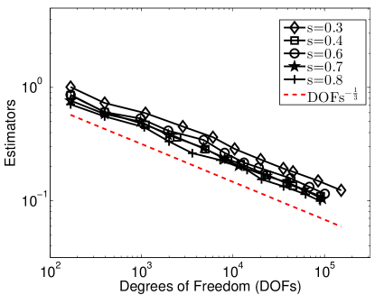
The results of Figure 1 show that the AFEM proposed in Section 6.1 delivers optimal experimental rates of convergence for the total error estimator $\mathfrak{E}$ and all choices of the parameter $s$ considered.

Fig. 1: Computational rates of convergence for our anisotropic AFEM with incompatible desired data $\mathsf{u}_{d}$ and a non-convex domain $\Omega=(-1,1)^{2}\setminus(0,1)\times(-1,0)$: $n=2$ and $s\in\{0.3,0.4,0.6,0.7,0.8\}$. The panel shows the decrease of the total error indicator $\mathfrak{E}$ with respect to the number of degrees of freedom (DOFs). In all the presented cases the optimal rate $(\#\mathscr{T}_{\mathpzc{Y}})^{-1/3}$ is achieved.

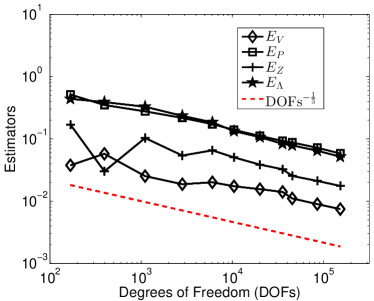
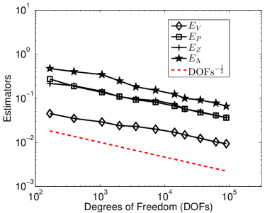
In Figure 2 we present, for $s=0.3$ (left) and $s=0.9$ (right), the computational rates of convergence for each of the four contributions of the computable error estimator $\mathcal{E}_{ocp}$: $\mathcal{E}_{V}$, $\mathcal{E}_{P}$, $\mathcal{E}_{Z}$, and $\mathcal{E}_{\Lambda}$. It can be observed that, in both cases, each contribution decays with the optimal rate $\#(\mathscr{T}_{\mathpzc{Y}})^{-1/3}$.

Fig. 2: Computational rates of convergence for the contributions $\mathcal{E}_{V}$, $\mathcal{E}_{P}$, $\mathcal{E}_{Z}$, and $\mathcal{E}_{\Lambda}$ of the computable and anisotropic a posteriori error estimator $\mathcal{E}_{ocp}$. We have considered $n=2$, an incompatible desired data $\mathsf{u}_{d}$, and a non-convex domain $\Omega=(-1,1)^{2}\setminus(0,1)\times(-1,0)$. The panels show the decrease of the contributions $\mathcal{E}_{V}$, $\mathcal{E}_{P}$, $\mathcal{E}_{Z}$, and $\mathcal{E}_{\Lambda}$ with respect to the number of degrees of freedom for $s=0.3$ (left panel) and $s=0.8$ (right panel). In both cases we recover the optimal rate $(\#\mathscr{T}_{\mathpzc{Y}})^{-1/3}$ for each contribution.

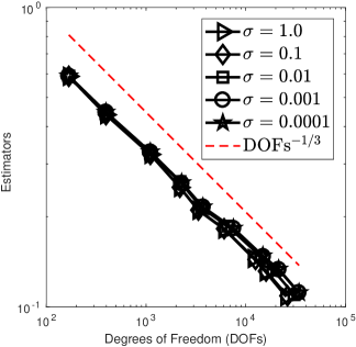
We now investigate the effect of varying the regularization parameter $\sigma$ by considering $s=0.8$, $\mathsf{a}=-0.3$, $\mathsf{b}=0.3$, $\theta=0.5$, $\nu=0.2$, and

$$\sigma\in\{10^{0},10^{-1},10^{-2},10^{-3},10^{-4}\}.$$

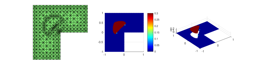
In Figure 3, we observe that optimal experimental rates of convergence are obtained for the error estimator $\mathcal{E}_{ocp}$ for all the values of the parameter $\sigma$ considered. In Figure 4 we present the adaptive mesh obtained by our AFEM after 9 iterations and the corresponding finite element approximations of the optimal control variable $\bar{\mathsf{z}}$ (a bang–bang controller).

Fig. 3: Computational rates of convergence for our anisotropic AFEM with incompatible desired data $\mathsf{u}_{d}$ and a non-convex domain $\Omega=(-1,1)^{2}\setminus(0,1)\times(-1,0)$: $n=2$, $\nu=0.2$, and $\sigma\in\{10^{0},10^{-1},10^{-2},10^{-3},10^{-4}\}$. The panel shows the decrease of the total error indicator $\mathfrak{E}$ with respect to the number of degrees of freedom (DOFs). In all the presented cases the optimal rate $(\#\mathscr{T}_{\mathpzc{Y}})^{-1/3}$ is achieved.

Fig. 4: Adaptive mesh obtained by our anisotropic AFEM, after 11 iterations, with incompatible desired data $\mathsf{u}_{d}$ and a non-convex domain $\Omega=(-1,1)^{2}\setminus(0,1)\times(-1,0)$, and the corresponding finite element approximations of the optimal control variable $\bar{\mathsf{z}}$. We have considered the sparsity parameter $\nu=0.2$ and the regularization parameter $\sigma=10^{-4}$.

6.4 Conclusions

Several conclusions can be drawn:

1. Geometric singularities and fractional diffusion behavior: Since $\mathsf{u}_{d}=1$, $\mathsf{u}_{d}$ is an incompatible forcing term, when $s\in(0,\tfrac{1}{2}]$, for the adjoint equation $(-\Delta)^{s}\bar{\mathsf{p}}=\bar{\mathsf{u}}-\mathsf{u}_{d}$. Our results show that, when $s=0.2$ and $s=0.3$, the devised AFEM localizes an important density of degrees of freedom near the boundary of the domain $\Omega$ and also near the reentrant corner. This is to compensate the singular behavior (1.5)–(1.6) that is inherent to fractional diffusion with incompatible data. When $s=0.8$ and $s=0.9$, the incompatibility of the desired data is not longer active and then the optimal adjoint state do not exhibits boundary layers. Our AFEM is thus focused on resolving the reentrant corner.

2. Sparse optimal controls: The fact that the cost functional $J$ involves the term $\|\mathsf{z}\|_{L^{1}(\Omega)}$ leads to sparsely supported optimal controls. Figure 4 is a particular instance of this feature. In addition, it can be observed that the error estimator $\mathcal{E}_{ocp}$ also focuses on refining the interface, i.e., the boundary of the active set.

References

- [1] M. Abramowitz and I.A. Stegun. Handbook of mathematical functions with formulas, graphs, and mathematical tables, volume 55 of National Bureau of Standards Applied Mathematics Series. 1964.
- [2] A. Allendes, F. Fuica, and E. Otárola. Adaptive finite element methods for sparse PDE–constrained optimization. IMA J. Numer. Anal., 2019. (accepted for publication) arXiv:1712.00448.
- [3] A. Allendes, E. Otárola, R. Rankin, and A. J. Salgado. Adaptive finite element methods for an optimal control problem involving Dirac measures. Numer. Math., 137(1):159–197, 2017.
- [4] A. Antil and E. Otárola. An a posteriori error analysis for an optimal control problem involving the fractional laplacian. IMA J. Numer. Anal., 38(1):198–226, 2018.
- [5] H. Antil and E. Otárola. A FEM for an optimal control problem of fractional powers of elliptic operators. SIAM J. Control Optim., 53(6):3432–3456, 2015.
- [6] H. Antil, E. Otárola, and A. J. Salgado. Optimization with respect to order in a fractional diffusion model: analysis, approximation and algorithmic aspects. J. Sci. Comput., 77(1):204–224, 2018.
- [7] I. Babuška and A. Miller. A feedback finite element method with a posteriori error estimation. I. The finite element method and some basic properties of the a posteriori error estimator. Comput. Methods Appl. Mech. Engrg., 61(1):1–40, 1987.
- [8] L. Banjai, J.M. Melenk, R.H. Nochetto, E. Otárola, A.J. Salgado, and Ch. Schwab. Tensor FEM for spectral fractional diffusion. Found. Comput. Math., 2018. (accepted for publication).
- [9] M. Š. Birman and M. Z. Solomjak. Spektralnaya teoriya samosopryazhennykh operatorov v gilbertovom prostranstve. Leningrad. Univ., Leningrad, 1980.
- [10] S. C. Brenner and L. R. Scott. The mathematical theory of finite element methods, volume 15 of Texts in Applied Mathematics. Springer, New York, third edition, 2008.
- [11] A. Bueno-Orovio, D. Kay, V. Grau, B. Rodriguez, and K. Burrage. Fractional diffusion models of cardiac electrical propagation: role of structural heterogeneity in dispersion of repolarization. J. R. Soc. Interface, 11(97), 2014.
- [12] X. Cabré and J. Tan. Positive solutions of nonlinear problems involving the square root of the Laplacian. Adv. Math., 224(5):2052–2093, 2010.
- [13] L. Caffarelli and L. Silvestre. An extension problem related to the fractional Laplacian. Comm. Part. Diff. Eqs., 32(7-9):1245–1260, 2007.
- [14] L. Caffarelli and A. Vasseur. Drift diffusion equations with fractional diffusion and the quasi-geostrophic equation. Ann. of Math., 171:1903–1930, 2010.
- [15] L. A. Caffarelli and P. R. Stinga. Fractional elliptic equations, Caccioppoli estimates and regularity. Ann. Inst. H. Poincaré Anal. Non Linéaire, 33(3):767–807, 2016.
- [16] A. Capella, J. Dávila, L. Dupaigne, and Y. Sire. Regularity of radial extremal solutions for some non-local semilinear equations. Comm. Part. Diff. Eqs., 36(8):1353–1384, 2011.
- [17] C. Carstensen and S. A. Funken. Fully reliable localized error control in the FEM. SIAM J. Sci. Comput., 21(4):1465–1484 (electronic), 1999.
- [18] E. Casas, R. Herzog, and G. Wachsmuth. Optimality conditions and error analysis of semilinear elliptic control problems with cost functional. SIAM J. Optim., 22(3):795–820, 2012.
- [19] J. M. Cascón and R. H. Nochetto. Quasioptimal cardinality of AFEM driven by nonresidual estimators. IMA J. Numer. Anal., 32(1):1–29, 2012.
- [20] L. Chen. FEM: An integrated finite element methods package in matlab. Technical report, University of California at Irvine, 2009.
- [21] L. Chen, R. H. Nochetto, E. Otárola, and A. J. Salgado. A PDE approach to fractional diffusion: a posteriori error analysis. J. Comput. Phys., 293:339–358, 2015.
- [22] W. Chen. A speculative study of -order fractional laplacian modeling of turbulence: Some thoughts and conjectures. Chaos, 16(2):1–11, 2006.
- [23] W. Chen and S. Holm. Fractional laplacian time-space models for linear and nonlinear lossy media exhibiting arbitrary frequency power-law dependency. The Journal of the Acoustical Society of America, 115(4):1424–1430, 2004.
- [24] P. G. Ciarlet. The finite element method for elliptic problems, volume 40 of Classics in Applied Mathematics. SIAM, Philadelphia, PA, 2002.
- [25] F. H. Clarke. Optimization and nonsmooth analysis, volume 5 of Classics in Applied Mathematics. Society for Industrial and Applied Mathematics (SIAM), Philadelphia, PA, second edition, 1990.
- [26] M. Costabel and M. Dauge. General edge asymptotics of solutions of second-order elliptic boundary value problems. I, II. Proc. Roy. Soc. Edinburgh Sect. A, 123(1):109–155, 157–184, 1993.
- [27] M. D’Elia, C. Glusa, and E. Otárola. A priori error estimates for the optimal control of the integral fractional laplacian. SIAM J. Control Optim., 2019. (accepted for publication) arXiv:1810.04262.
- [28] Q. Du, M. Gunzburger, R.B. Lehoucq, and K. Zhou. Analysis and approximation of nonlocal diffusion problems with volume constraints. SIAM Rev., 54(4):667–696, 2012.
- [29] J. Duoandikoetxea. Fourier analysis, volume 29 of Graduate Studies in Mathematics. American Mathematical Society, Providence, RI, 2001.
- [30] R. G. Durán and A. L. Lombardi. Error estimates on anisotropic elements for functions in weighted Sobolev spaces. Math. Comp., 74(252):1679–1706 (electronic), 2005.
- [31] A. Ern and J.-L. Guermond. Theory and practice of finite elements, volume 159 of Applied Mathematical Sciences. Springer-Verlag, New York, 2004.
- [32] E. B. Fabes, C.E. Kenig, and R.P. Serapioni. The local regularity of solutions of degenerate elliptic equations. Comm. Part. Diff. Eqs., 7(1):77–116, 1982.
- [33] P. Gatto and J.S. Hesthaven. Numerical approximation of the fractional laplacian via hp-finite elements, with an application to image denoising. J. Sci. Comp., 65(1):249–270, 2015.
- [34] C. Glusa and E. Otárola. Optimal control of a parabolic fractional PDE: analysis and discretization. arXiv:1905.10002, 2019.
- [35] V. Gol′dshtein and A. Ukhlov. Weighted Sobolev spaces and embedding theorems. Trans. Amer. Math. Soc., 361(7):3829–3850, 2009.
- [36] P. Grisvard. Elliptic problems in nonsmooth domains, volume 24 of Monographs and Studies in Mathematics. Pitman (Advanced Publishing Program), Boston, MA, 1985.
- [37] M. Hintermüller, R. H. W. Hoppe, Y. Iliash, and M. Kieweg. An a posteriori error analysis of adaptive finite element methods for distributed elliptic control problems with control constraints. ESAIM Control Optim. Calc. Var., 14(3):540–560, 2008.
- [38] R. Ishizuka, S.-H. Chong, and F. Hirata. An integral equation theory for inhomogeneous molecular fluids: The reference interaction site model approach. J. Chem. Phys, 128(3), 2008.
- [39] K. Kohls, A. Rösch, and K. G. Siebert. A posteriori error analysis of optimal control problems with control constraints. SIAM J. Control Optim., 52(3):1832–1861, 2014.
- [40] N. S. Landkof. Foundations of modern potential theory. Springer-Verlag, New York, 1972. Translated from the Russian by A. P. Doohovskoy, Die Grundlehren der mathematischen Wissenschaften, Band 180.
- [41] S. Z. Levendorskiĭ. Pricing of the American put under Lévy processes. Int. J. Theor. Appl. Finance, 7(3):303–335, 2004.
- [42] W. Liu and N. Yan. A posteriori error estimates for distributed convex optimal control problems. Adv. Comput. Math., 15(1-4):285–309 (2002), 2001. A posteriori error estimation and adaptive computational methods.
- [43] P. Morin, R. H. Nochetto, and K. G. Siebert. Data oscillation and convergence of adaptive FEM. SIAM J. Numer. Anal., 38(2):466–488 (electronic), 2000.
- [44] P. Morin, R.H. Nochetto, and K.G. Siebert. Local problems on stars: a posteriori error estimators, convergence, and performance. Math. Comp., 72(243):1067–1097 (electronic), 2003.
- [45] B. Muckenhoupt. Weighted norm inequalities for the Hardy maximal function. Trans. Amer. Math. Soc., 165:207–226, 1972.
- [46] R. Musina and A. I. Nazarov. On fractional Laplacians. Comm. Partial Differential Equations, 39(9):1780–1790, 2014.
- [47] R. H. Nochetto, E. Otárola, and A. J. Salgado. A PDE approach to fractional diffusion in general domains: a priori error analysis. Found. Comput. Math., 15(3):733–791, 2015.
- [48] R. H. Nochetto, E. Otárola, and A. J. Salgado. Piecewise polynomial interpolation in Muckenhoupt weighted Sobolev spaces and applications. Numer. Math., 132(1):85–130, 2016.
- [49] R. H. Nochetto, K. G. Siebert, and A. Veeser. Theory of adaptive finite element methods: an introduction. In Multiscale, nonlinear and adaptive approximation, pages 409–542. Springer, Berlin, 2009.
- [50] E. Otárola. A PDE approach to numerical fractional diffusion. ProQuest LLC, Ann Arbor, MI, 2014. Thesis (Ph.D.)–University of Maryland, College Park.
- [51] E. Otárola. A piecewise linear FEM for an optimal control problem of fractional operators: error analysis on curved domains. ESAIM Math. Model. Numer. Anal., 51(4):1473–1500, 2017.
- [52] E. Otárola and A. J. Salgado. Sparse optimal control for fractional diffusion. Comput. Methods Appl. Math., 18(1):95–110, 2018.
- [53] H. Pham. Optimal stopping, free boundary, and American option in a jump-diffusion model. Appl. Math. Optim., 35(2):145–164, 1997.
- [54] W. Schirotzek. Nonsmooth analysis. Universitext. Springer, Berlin, 2007.
- [55] R. Schneider and G. Wachsmuth. A Posteriori Error Estimation for Control-Constrained, Linear-Quadratic Optimal Control Problems. SIAM J. Numer. Anal., 54(2):1169–1192, 2016.
- [56] S.A. Silling. Why peridynamics? In Handbook of peridynamic modeling, Adv. Appl. Math. CRC Press, 2017.
- [57] L. Silvestre. Regularity of the obstacle problem for a fractional power of the Laplace operator. Comm. Pure Appl. Math., 60(1):67–112, 2007.
- [58] G. Stadler. Elliptic optimal control problems with -control cost and applications for the placement of control devices. Comput. Optim. Appl., 44(2):159–181, 2009.
- [59] E. M. Stein. Singular integrals and differentiability properties of functions. Princeton Mathematical Series, No. 30. Princeton University Press, Princeton, N.J., 1970.
- [60] F. Tröltzsch. Optimal control of partial differential equations, volume 112 of Graduate Studies in Mathematics. American Mathematical Society, Providence, RI, 2010. Theory, methods and applications, Translated from the 2005 German original by Jürgen Sprekels.
- [61] B. O. Turesson. Nonlinear potential theory and weighted Sobolev spaces, volume 1736 of Lecture Notes in Mathematics. Springer-Verlag, Berlin, 2000.
- [62] R. Verfürth. A Review of A Posteriori Error Estimation and Adaptive Mesh-Refinement Techniques. John Wiley, 1996.
- [63] G. Wachsmuth and D. Wachsmuth. Convergence and regularization results for optimal control problems with sparsity functional. ESAIM Control Optim. Calc. Var., 17(3):858–886, 2011.