Topological Singularity Induced Chiral Kohn Anomaly in a Weyl Semimetal

Abstract

The electron-phonon interaction (EPI) is instrumental in a wide variety of phenomena in solid-state physics, such as electrical resistivity in metals Pines and Nozières (1999), carrier mobility, optical transition and polaron effects in semiconductors Ridley (2013); Elliott (1957), lifetime of hot carriers Allen (1987); Tisdale et al. (2010); Kozawa et al. (2014), transition temperature in BCS superconductors Schrieffer (1999), and even spin relaxation in diamond nitrogen-vacancy centers for quantum information processing Wrachtrup and Jelezko (2006); Fu et al. (2009); Jarmola et al. (2012). However, due to the weak EPI strength, most phenomena have focused on electronic properties rather than on phonon properties. One prominent exception is the Kohn anomaly, where phonon softening can emerge when the phonon wavevector nests the Fermi surface of metals Kohn (1959). Here we report a new class of Kohn anomaly in a topological Weyl semimetal (WSM), predicted by field-theoretical calculations, and experimentally observed through inelastic x-ray and neutron scattering on WSM tantalum phosphide (TaP). Compared to the conventional Kohn anomaly, the Fermi surface in a WSM exhibits multiple topological singularities of Weyl nodes, leading to a distinct nesting condition with chiral selection, a power-law divergence, and non-negligible dynamical effects. Our work brings the concept of Kohn anomaly into WSMs and sheds light on elucidating the EPI mechanism in emergent topological materials.

In 1959, Walter Kohn proposed the anomalous phonon dispersion behavior in a metal, which arises when electrons lose their dielectric screening Kohn (1959). This anomaly, known as a Kohn anomaly, directly images the Fermi surface on the phonon dispersion, and overturned the long belief that the weak EPI can only lead to negligible effects on phonon properties. Intuitively, a Kohn anomaly occurs when electronic states $\bm{k}_{1}$ and $\bm{k}_{2}$ near the Fermi surface are parallelly nested by a phonon with wavevector $\bm{q}\equiv\bm{k}_{2}-\bm{k}_{1}$. This is a stringent condition only met by a single $q\equiv|\bm{q}|$ value at $q\approx 2k_{F}$, where $k_{F}$ is the Fermi wavevector. Extensive research has delved into the role of Kohn anomalies in conventional Aynajian et al. (2008) and unconventional superconductors Weber (1987); Reznik et al. (2006), carbon materials such as carbon nanotubes Piscanec et al. (2007), graphene Mafra et al. (2009); Tse et al. (2008); Wunsch et al. (2006), and graphite Ferrari (2007), as well as other low-dimensional systems such as 1D conductors Renker et al. (1973) and topological insulators Zhu et al. (2012).

The recent development of WSMs Xu et al. (2015); Lv et al. (2015); Weng et al. (2015); Huang et al. (2015); Min et al. (2019) offers a new platform to realize exotic phonon properties, such as the phonon Hall effect Cortijo et al. (2015), chiral magnetic effect Song et al. (2016) and chiral anomaly in phonon spectra Rinkel et al. (2017). As such, WSMs could serve as an intriguing platform to study Kohn anomalies due to the presence of topologically protected Weyl nodes and 3D linear-dispersive Weyl fermions.

In this Letter, we theoretically predict and experimentally observe a new type of Kohn anomaly in WSM, which exhibits a few novel features. First, since the simply-connected Fermi surface in a conventional Fermi liquid evolves into disconnected topological singularities of chiral Weyl nodes, the condition to achieve Kohn anomalies becomes largely relaxed. As the EPI does not change chirality, it plays an essential role in understanding the coupling strength through the following requisite. For two Weyl nodes located at $\bm{k}_{W1}$ and $\bm{k}_{W2}$, both which necessarily share the same chirality, a phonon with $\bm{q}\approx\bm{k}_{W2}-\bm{k}_{W1}$ can directly lead to the anomaly. In particular, for our chosen material of type-I WSM TaP, which contains two sets of inequivalent Weyl nodes $\{\bm{k}_{W1}\}$ and $\{\bm{k}_{W2}\}$, there is a subset of nodes satisfying $\bm{k}_{W2}-\bm{k}_{W1}\in\{\bm{k}_{W2}\}$ Weng et al. (2015). As a result, phonon $\bm{q}$ values can be chosen directly at Weyl nodes. Second, instead of a logarithmic divergence as in a Fermi liquid or a weak power-law divergence as in graphene Hwang and Das Sarma (2008), the Kohn anomaly in a WSM shows a stronger power-law divergence. This counterintuitive result originates from the 3D dispersion. Third, in WSM, the Debye frequency $\omega_{D}$ can be higher than the Fermi level $E_{F}$, indicating a non-negligible dynamical effect, since the frequency dependence of the dielectric function occurs on the scale of $\omega_{D}$. Such a dynamical effect leads to softening within a finite regime in the Brillouin zone instead of at an individual $\bm{q}$ point. This contrasts with the conventional Fermi liquid, where static screening suffices since $\omega_{D}\ll E_{F}$. Our work represents the first reported observation of a Kohn anomaly in a topological nodal semimetal, and offers a new tool for probing the EPI characteristics in a broader category of topological materials.

Field-theoretical calculation of topological Kohn anomaly. The dielectric screening from inter-node scattering via a phonon $\bm{q}=\bm{k}_{W2}-\bm{k}_{W1}$ is computed for 3D linear dispersive Weyl fermions using $E(\bm{k})=\pm v_{F}|\bm{k}-\bm{k}_{Wj}|-\mu_{j}$, where $v_{F}$ is the Fermi velocity and $j=1,2$ denotes different Weyl nodes at chemical potential $\mu_{j}$. The polarization operator $\Pi(\nu,\bm{q})$ from the inter-Weyl-node scattering can be written as (Supplementary A 1):

where $q^{\prime}=|\bm{q}+\bm{k}_{W1}-\bm{k}_{W2}|$, $\nu^{\prime}=\nu-\mu_{1}+\mu_{2}$ and $\Lambda$ is a momentum cutoff. Since the dynamical dielectric function $\epsilon_{r}(\nu,\bm{q})$ can be written as $\epsilon_{r}(\nu,\bm{q})=1-4\pi e^{2}\Pi(\nu,\bm{q})/(\kappa q^{2})$, we see immediately that a Kohn anomaly with a strong power-law divergence can occur with the following condition

$$v_{F}q^{\prime}=\pm\nu^{\prime}.$$ (2)

by satisfying which the momentum derivative of dielectric function diverges:

$$\frac{\partial\varepsilon_{r}}{\partial q}\propto\frac{\left(v_{F}q^{\prime}\right)^{3}}{\left(v_{F}q^{\prime}\right)^{2}-(\nu^{\prime})^{2}}.$$ (3)

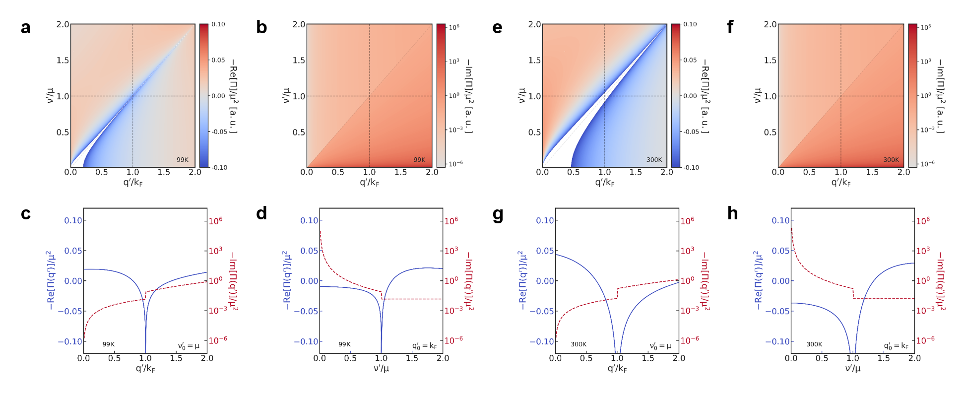
Figure S1: Density plot of the a, real, and the b, imaginary part of the polarization function $-\Pi(\bm{q}^{\prime},\nu^{\prime})$ at 99K and with finite doping where $\bm{q}^{\prime}=\bm{q}-\bm{k}_{W1}+\bm{k}_{W2}$ and $\nu^{\prime}=\nu-\mu_{1}+\mu_{2}$. c. Line profile of negative $\textrm{Re}[\Pi(\bm{q}^{\prime},\nu_{0}^{\prime}=\mu)]$ and $\textrm{Im}[\Pi(\bm{q}^{\prime},\nu_{0}^{\prime}=\mu)]$ at a constant frequency $\nu_{0}^{\prime}/\mu=1$. d. Line profile of negative $\textrm{Re}[\Pi(q_{0}^{\prime}=k_{F},\nu^{\prime})]$ and $\textrm{Im}[\Pi(q_{0}^{\prime}=k_{F},\nu^{\prime})]$ at a constant wavevector $q_{0}^{\prime}/k_{F}=1$, where divergence at $\mathrm{v}_{F}q^{\prime}=\nu^{\prime}$ is maintained. e-h. Analogous to subfigures a-d, calculated at a temperature of 300K.

The divergence condition for a Kohn anomaly implies that the momentum mismatch $\delta\bm{q}\equiv\bm{q}-(\bm{k}_{W2}-\bm{k}_{W1})$ can be compensated by a finite dynamical effect $\nu^{\prime}$. Consequentially, a patch of $\bm{q}$ values in momentum space with small momentum mismatch can still experience a Kohn anomaly. In fact, the simple divergence condition $v_{F}q^{\prime}=\pm\nu^{\prime}$ will persist even with finite doping. The density plots of the real and imaginary parts of $-\Pi(\nu,\bm{q})$ at finite doping and temperature are shown in Figures 1a and 1b (additional temperatures in Figures S1 and S2). The divergence appears as a sharp peak along the line $v_{F}q^{\prime}=\nu^{\prime}$, and is further visualized along constant-frequency $\nu_{0}^{\prime}/\mu=1$ and constant-wavevector $q_{0}^{\prime}/k_{F}=1$ cuts in Figures 1c and 1d, respectively in reduced dimensionless units, where $\mu\equiv\sqrt{\mu_{1}^{2}+\mu_{2}^{2}}$, and $k_{F}\equiv\mu/v_{F}$. Figure 1e is a plot of $-\text{Re}[\Pi(\nu,\bm{q})]$ in $\bm{\delta q}_{x}$–$\bm{\delta q}_{y}$ space integrated from 0 to $\nu^{\prime}$, which is proportional to the magnitude of the phonon softening and reveals a negative contribution emanating from the zero-mismatch condition as a result of the divergence at $v_{F}q^{\prime}=\pm\nu^{\prime}$. The divergence is alleviated here by a small numerical imaginary part mimicking the considerations of additional scattering terms. Line cuts in $\bm{\delta q}_{x}$–$\bm{\delta q}_{y}$ space shown in Figure 1f reveal a broad dip in $-\text{Re}[\Pi(\nu,\bm{q})]$ that does not necessarily occur at the zero-mismatch condition, thereby demonstrating the existence of a non-negligible dynamical effect. It is worthwhile mentioning that although the polarization in Figure 1c and 1d shows a sharp divergence, the distinct condition to fulfill a Kohn anomaly in a patch of $\bm{q}$ values eventually leads to a broad "bowl-shaped" softening in the Brillouin zone, which qualitatively agrees well with the experiments without knowing the EPI coupling constants. The EPI, embodied through an expression for $\Pi(\nu,\bm{q})$ characteristic of WSMs, results in an distinct renormalization of the bare ionic phonon frequencies within a range of $\bm{q}$-space conducive to a different nature of Kohn anomaly.

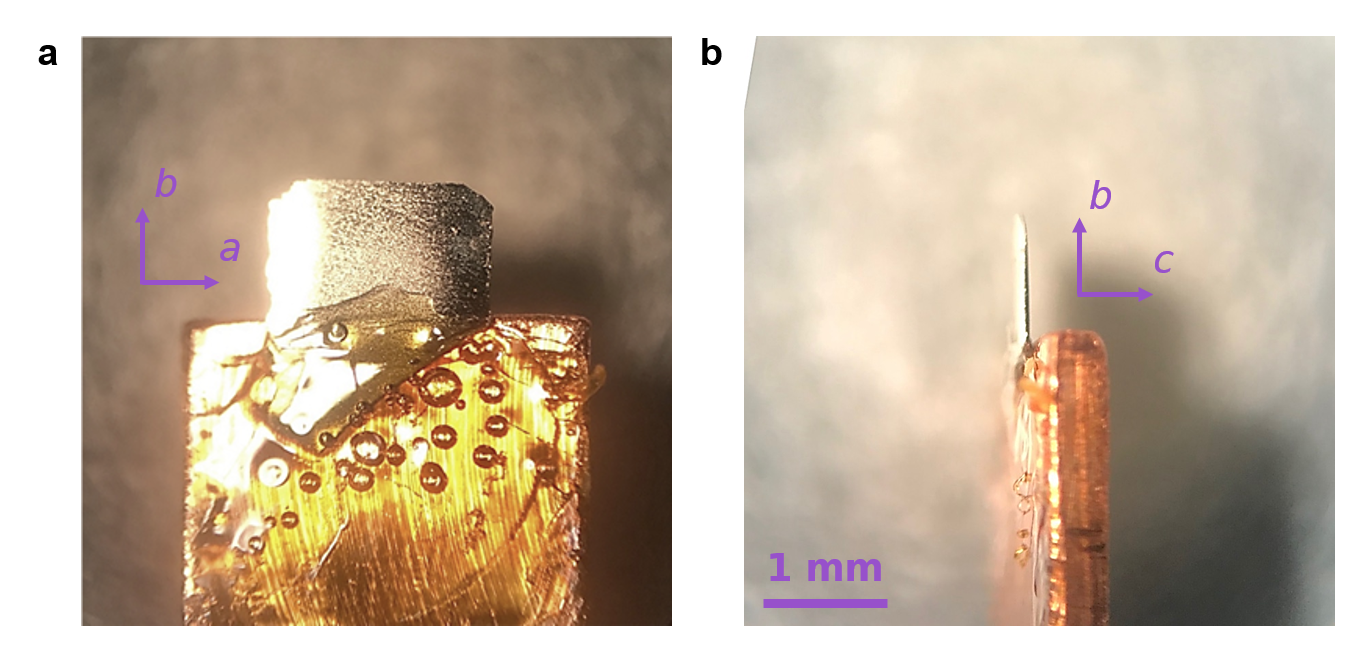
Figure S3: a, Top view and b, side view of the orientated and thinned-down tantalum phosphide (TaP) sample used for the IXS experiments.

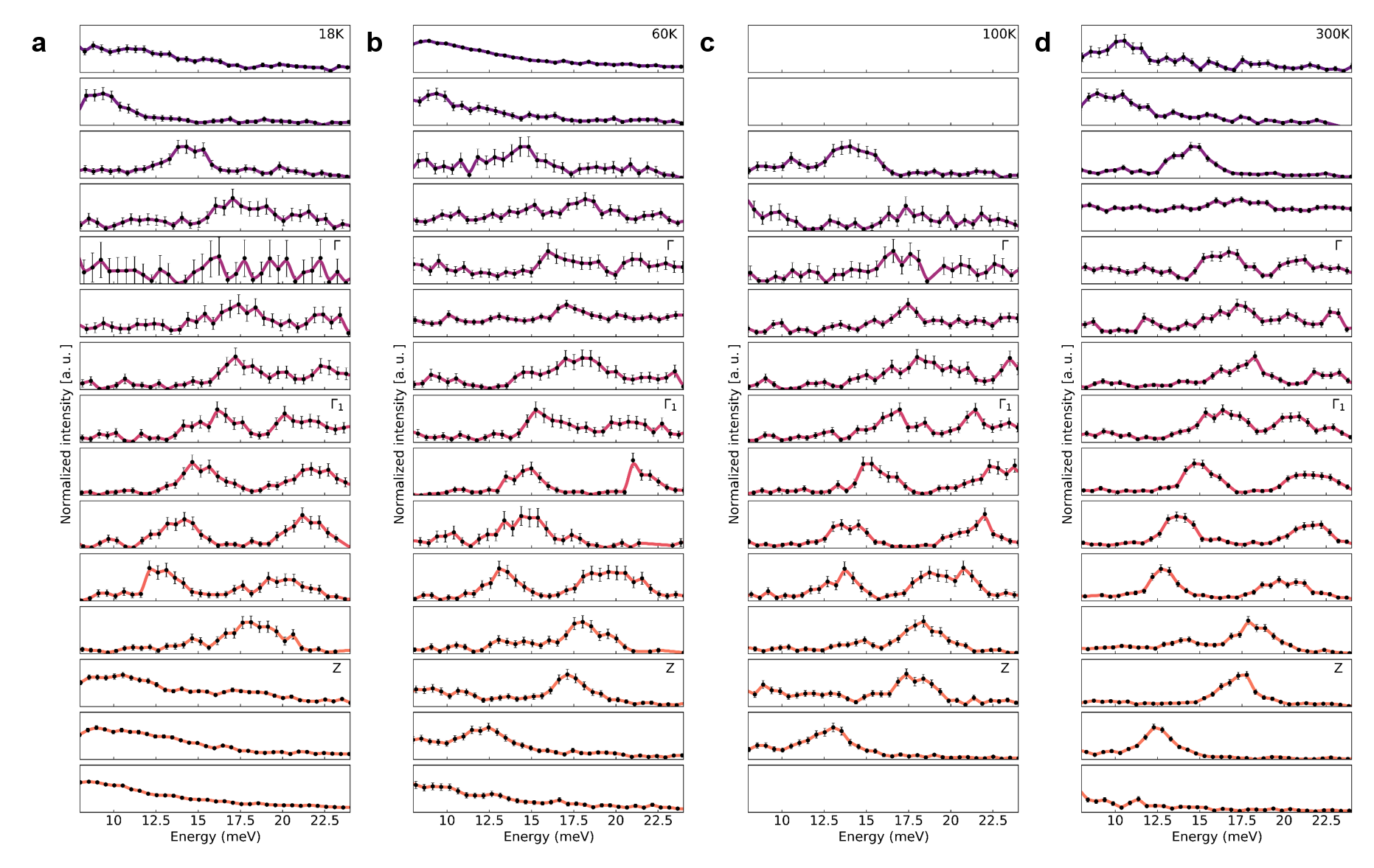
Figure S4: From top to bottom of each subfigure, intensity spectra obtained from IXS measurements performed along high-symmetry loop $\Gamma$-$\Sigma$-$\Sigma_{1}$-Z-$\Gamma$ at a, 18K, b, 60K, c, 100K and d, 300K. Lines serve as a guide to the eye.

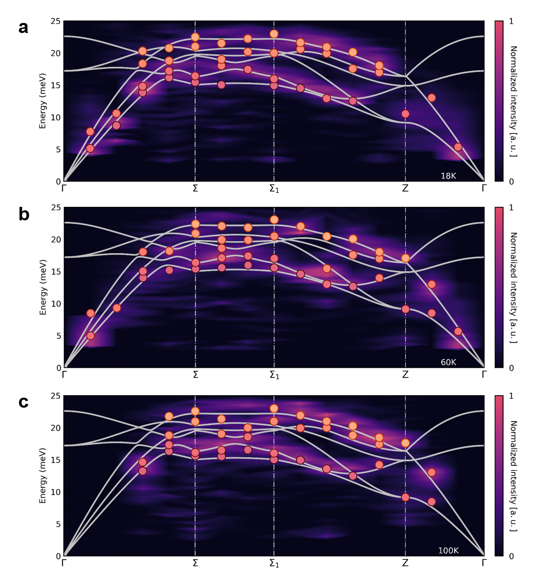
Figure S6: Experimental phonon dispersion of TaP encompassing the three acoustic phonon modes and the three lowest-energy optical modes along high symmetry loop $\Gamma$-$\Sigma$-$\Sigma_{1}$-Z-$\Gamma$ at a, 18K, b, 60K and c, 100K. The points represent extracted phonon modes from intensity spectra at that $\bm{q}$-value in momentum space. The grey lines are ab initio calculations of the phonon dispersion. The color map shows the intensities of the phonon modes extracted from the intensity spectra following removal of the elastic peak. The first two and the last $\bm{q}$-values along the high-symmetry loop of the 100K phonon dispersion were not measured.

Phonon dispersion along high-symmetry directions. TaP crystallizes in the body-centered tetragonal space group I4₁md (109) (Figure 2a) and hosts two sets of inequivalent Weyl nodes, denoted W1 and W2 (Figure 2b). We first present the phonon dispersion measurements of a TaP crystal (Figure S3, Supplementary B and C 2) along a high-symmetry loop $\Gamma$-$\Sigma$-$\Sigma_{1}$-Z-$\Gamma$ (Figure 2c with data in Figure S4) using inelastic X-ray scattering (IXS). We focused on the low-energy phonons ($<$25 meV), which include the Ta optical phonons but not those associated with the motion of P atoms. The phonon energies are extracted using damped harmonic oscillator models to convolute with the instrument resolution functions, and then fitting the measured spectra. The resulting phonon dispersion is shown in Figure 2d (and Figure S6 for lower temperatures), along which the intensity of fitting the intrinsic scattering (after deconvolution) is plotted as a color map. Grey lines designate ab initio phonon dispersion calculations for which the procedure is detailed in Supplementary D 3. Further data were collected using inelastic neutron scattering (INS), which agrees well with the dispersion from IXS (Figure S7). The excellent agreement between experiments and ab initio calculations indicates a level of reliability of computational phonon spectra, which serves as a basis to compare phonon dispersions away from high-symmetry lines.

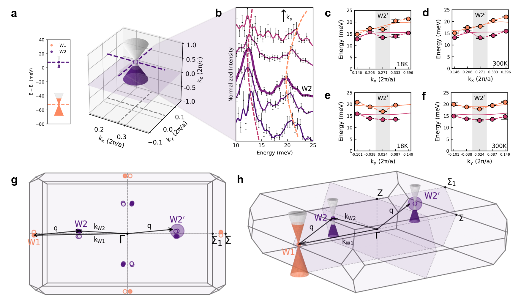
Figure 3: Topological Kohn anomaly at W2 Weyl node. a. Location of the W2 Weyl node in energy and momentum space. b. Phonon spectra near the W2 Weyl node, with central thicker line denoting the location of W2^′. Strong phonon softening at this Weyl node is observed. c-f. Dispersion of two representative phonon modes near W2 at 18K and 300K, along $k_{x}$ and $k_{y}$ directions. Solid lines correspond to ab initio calculations without the EPI, where their discrepancy with experimental data further supports the strong softening near the W2 node. 2D (g) and 3D (h) showing the realization condition of Kohn anomaly, where a phonon $\bm{q}=\bm{k}_{W2}-\bm{k}_{W1}\approx\bm{k}_{W2^{\prime}}$ connects two Weyl nodes $\bm{k}_{W1}$ and $\bm{k}_{W2}$.

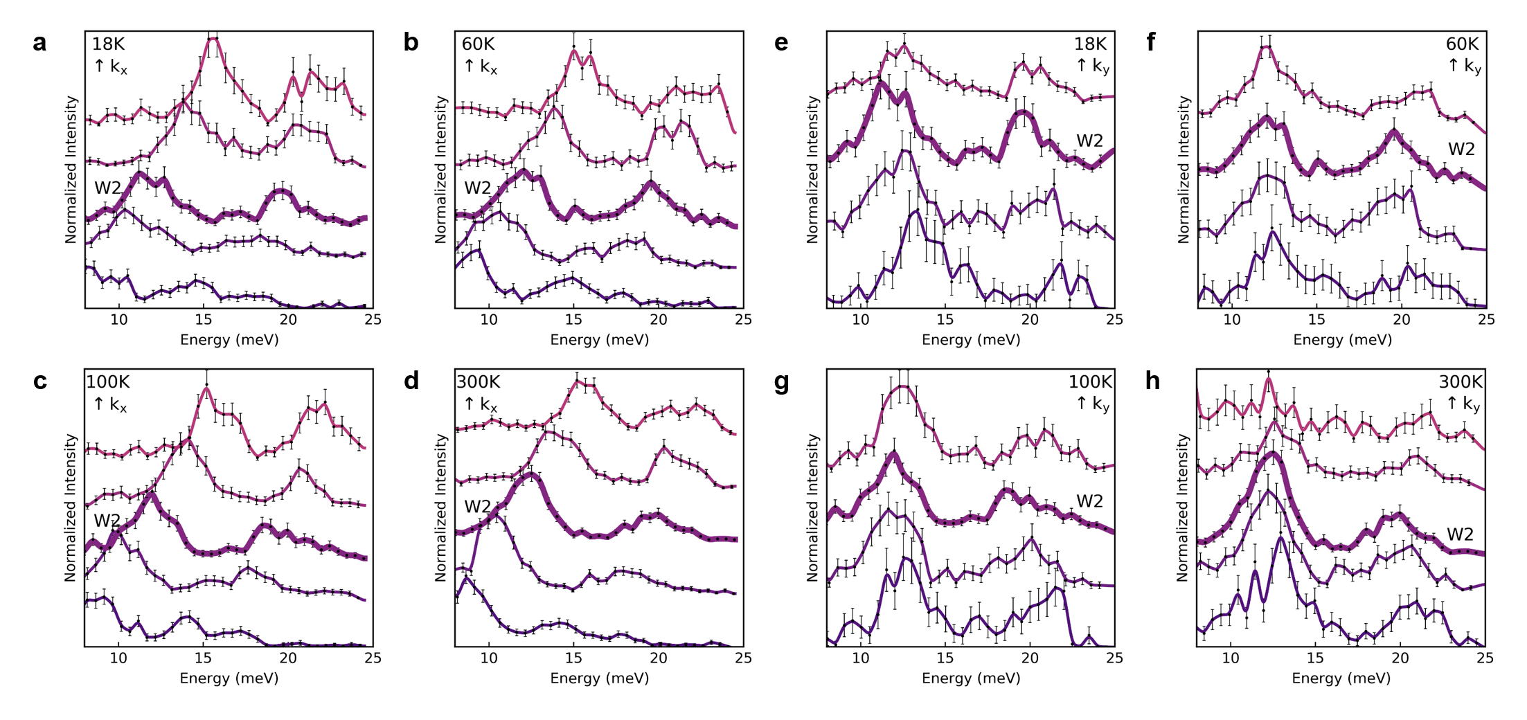
Figure S8: Momentum dependence of the intensity spectra with statistical error near the W2 Weyl node at $(0.271,0.024,0.578)$ (denoted as $\bm{k}_{W2^{\prime}}$ in main text). a-d display the IXS intensity spectra for $\bm{q}$-values along $H$ in $(H,0.024,0)$ for increasing $k_{x}$ direction from bottom to top at 18K, 60K, 100K and 300K, respectively. e-h display similar measurements at the same temperatures for $\bm{q}$-values along $K$ in $(0.271,K,0)$ for increasing $k_{y}$ direction from bottom to top. There are only four measurements due to instrumental limitations for larger $\bm{q}$-values, except for 300K. Lines serve as a guide to the eye. The central thicker line in each of the subfigures represents the IXS measurement performed directly at the W2 node.

Observation of topological chiral Kohn anomaly. We present experimental signatures highlighting the presence of a Kohn anomaly at the W2 Weyl node, predicted in Figure 1. In our TaP sample, the W1 Weyl nodes are $\sim 60$meV below $E_{F}$ , while W2 nodes are a few meV above $E_{F}$ (Figure 3a). As a result, W1 represents a much larger carrier pocket than W2. We carried out IXS measurements at $\bm{q}$ values near a W2 Weyl node located at $\bm{k}_{W2^{\prime}}=(0.271,0.024,0.578)$ (Figure S8). Even without fitting, the phonon softening at the Weyl node can be seen clearly from the original data in Figure 3b. The bowl-shaped softening characteristics resembles the field-theoretical prediction in Figure 1f very well, although a quantitative agreement is unpractical, requiring the mode-resolved EPI contants. The fitted phonon dispersion relation of the highest acoustic and the lowest optical phonons along the $k_{x}$ and $k_{y}$ directions within the plane containing $\bm{k}_{W2^{\prime}}$ are shown in Figures 3c-3f. Strong phonon softening is observed at both $T=18$K and $T=300$K, and in both $k_{x}$ and $k_{y}$ directions. Such softening is absent in ab initio calculations without considering EPI. The semi-quantitative agreement between theory and experimental trends, the consistent softening behavior at multiple $\bm{q}$ points, and the absence of softening in ab initio calculations without EPI consideration, overall strongly suggest an EPI nature of the phonon softening. Additionally, the phonon softening takes place at all measured temperatures, indicating a possible topological robustness. Such softening can be understood as a Kohn anomaly from inter-Weyl node scattering. In fact, it is possible to nest a W1 electronic state at $\bm{k}_{W1}=(-0.518,-0.014,0)$ with another W2 state $\bm{k}_{W2}=(-0.271,0.024,0.578)$, both with "+" chirality, via a phonon $\bm{q}=\bm{k}_{W2}-\bm{k}_{W1}\approx\bm{k}_{W2^{\prime}}$, with a mismatch $|\bm{q}-\bm{k}_{W2^{\prime}}|/|\bm{k}_{W2^{\prime}}|\sim$ 4%. Details relating to different nesting combinations are listed in Supplementary E. The schematics of this nesting condition are shown in Figures 3g-3h. As mentioned previously, the dynamical effect significantly reduces the mismatch down to $\sim$ 1% and further enables the Kohn anomaly to manifest at $\bm{q}\simeq\bm{k}_{W2^{\prime}}$. In particular, the dynamical correlation almost exactly reproduces the strong phonon softening feature at Weyl node $\bm{k}_{W2^{\prime}}$: with $v_{F}\sim 1.5\times 10^{5}$m/s in TaP and the momentum mismatch being $v_{F}\delta\bm{q}\sim 50$meV, $\nu^{\prime}\sim 60$meV largely compensates for the mismatch, thereby facilitating the satisfaction of the divergence condition and agreeing with the observation in Figures 3c-3f.

Chirality selection of the topological chiral Kohn anomaly. The IXS measurements carried out near a W1 Weyl node (Figures 4a and S9) present a contrasting result. When the phonon $\bm{q}$ is near a W1 node $\bm{k}_{W1^{\prime}}=(0.518,0.014,0)$, there is no clear indication of phonon softening at all measured temperatures, where measured phonon dispersions agree very well with ab initio calculations in Figures 4b-4e). This is largely due to a lack of a scattering channel that can simultaneously conserve momentum and chirality. For momentum-conserved scattering, although the phonon nesting condition can still roughly be met by considering scattering from $\bm{k}_{W2}$ to $\bm{k}_{W2^{\prime}}$, where $\bm{q}=\bm{k}_{W2^{\prime}}-\bm{k}_{W2}=(0.542,0,0)\approx\bm{k}_{W1^{\prime}}$ (mismatch $|\bm{q}-\bm{k}_{W1^{\prime}}|/|\bm{k}_{W1^{\prime}}|\sim$ 5%) (Figure 4f), the W2 and W2^′ nodes have opposite chirality ("$+$" and "$-$", respectively), prohibiting the EPI to occur. On the other hand, for a chirality-conserved scattering $\bm{q}=\bm{k}_{W2^{\prime}}-\bm{k}_{\overline{W2}}$, where $\bm{k}_{\overline{W2}}=(-0.271,-0.024,0.578)$ gives the $\overline{\textrm{W2}}$ node paired with W2^′ and has "$-$" chirality, the $\sim 8\%$ momentum mismatch is simply too large to compensate even with dynamical effects considered. Moreover, the low carrier concentration of the hole pockets at W2 nodes further decreases the overall EPI contribution. As such, the magnitude of the Kohn anomaly at W1 should be imperceptible relative to the results at W2. This analysis corroborates the IXS data.

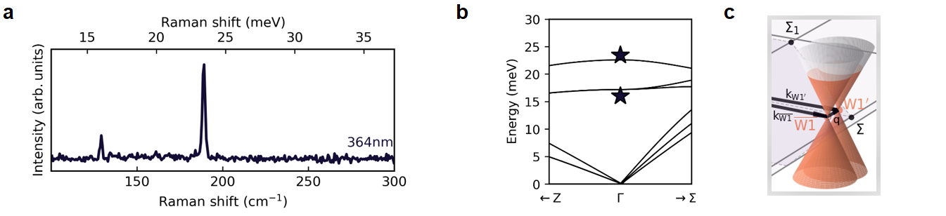
Figure S11: a. Raman peak shifts of TaP collected at room temperature at laser excitation 364nm. b. Comparison between Raman-measured phonon modes at the $\Gamma$ point and ab initio calculations, which is the same dispersion seen in Figure 1f. c. Close-up of the two W1 nodes near the zone boundary that connect as a small $\bm{q}\approx\Gamma$ vector.

In addition to the two types of Weyl nodes, one may expect a Kohn anomaly to emerge at the $\Gamma$ point. However, the chirality-conserved scattering channel (say, W1 and W1^′) has large momentum mismatch away from the $\Gamma$-point, while the momentum-conserved channel (say, W1^′ and $\overline{\textrm{W1}}$ with $\bm{k}_{\overline{W1}}=(0.518,-0.014,0)$ does not preserve chirality as shown in Figures S11. A mixed behavior is observed from Raman scattering measurements. A weak softening $\sim$ 1.2meV is observed for the lower optical phonon at the $\Gamma$-point, but not for the higher-energy optical phonon. As a result, the intra-node scattering may still happen and requires further investigation.

To summarize, we theoretically formulated and experimentally demonstrated a Kohn anomaly in a WSM, which can lead to the anomalous broad-range phonon softening behaviors arising from the scattering between the topological singularity of chiral Weyl nodes. Unlike a conventional Fermi liquid, in TaP, with 8 W1 nodes and 16 W2 nodes, numerous $\bm{q}$ regimes in the Brillouin zone can achieve Kohn anomalies. The recent ab initio calculations in Dirac semimetals also confirm the existence of Kohn anomalies in topological semimetals Yue et al. (2019, 2020). Moreover, in contrast to the conventional Fermi liquid with only static screening and logarithmic divergence $d\epsilon_{r}/dq\propto\ln(|q-2k_{F}|/4k_{F})$, or graphene and 2D electron gas with $\partial\epsilon_{r}/\partial q\propto 1/\sqrt{q^{2}-4k_{F}^{2}}$, we find a highly distinct divergence condition at $v_{F}q^{\prime}\rightarrow\pm\nu^{\prime}$ with a leading term $\partial\epsilon_{r}/\partial q\propto(v_{F}q^{\prime})^{3}/[(v_{F}q^{\prime})^{2}-\nu^{\prime 2}]$, where dynamical effects play a critical role with explicit Weyl node location dependence and chirality selection. The Kohn anomaly identified in our work highlights a previously overlooked instance of EPI in WSMs, and can offer a ubiquitous tool to extract the EPI strength, as carried out in graphite Piscanec et al. (2004), to elucidate the interplay between chiral Weyl fermions and phonons. Our discovery adds to the rich array of exotic EPI effects realized in novel topological materials.

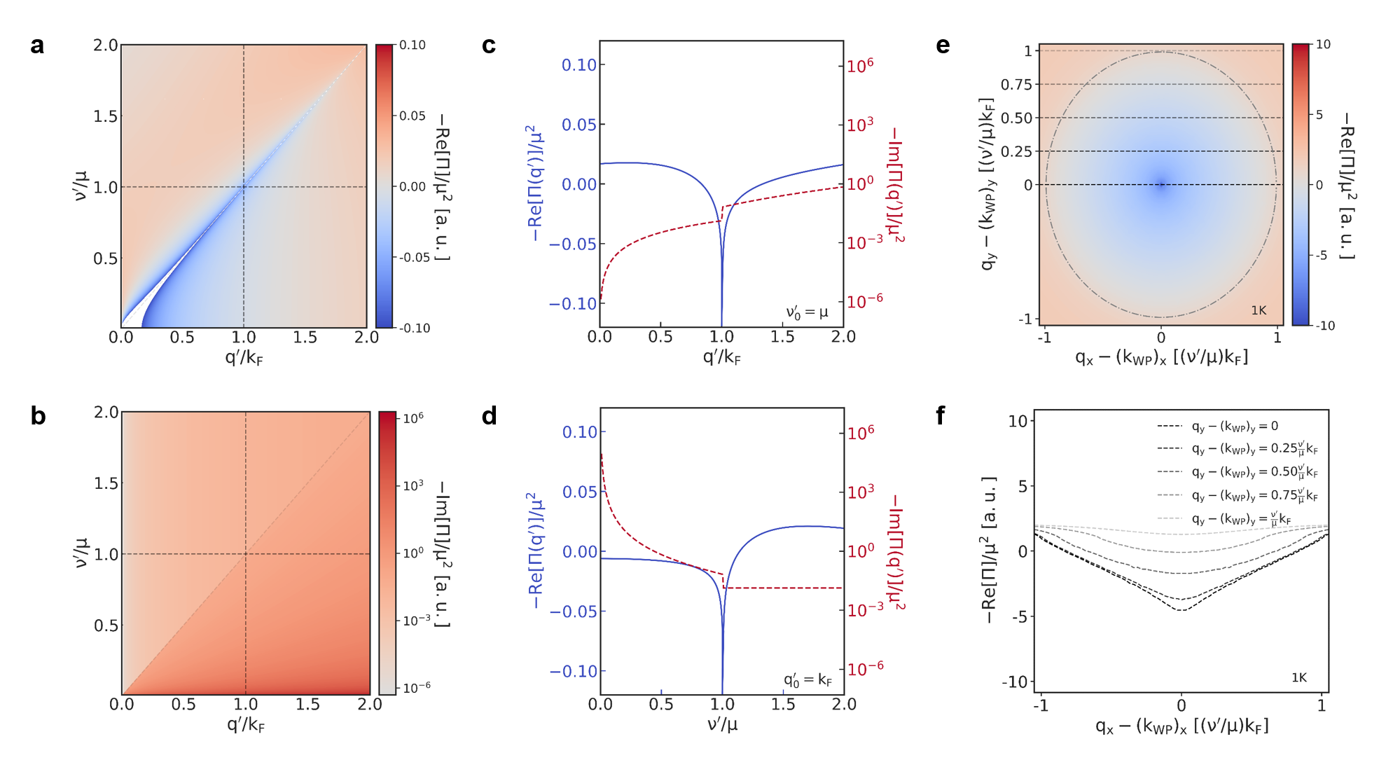
Figure 1: Field-theoretical calculations of topological Kohn anomaly. Density plot of the a, real, and the b, imaginary part of the polarization function $-\Pi(\bm{q}^{\prime},\nu^{\prime})$ at $T=1K$ c. Constant-frequency line profile of $-\textrm{Re}[\Pi(\bm{q}^{\prime},\nu_{0}^{\prime}=\mu)]$ and $-\textrm{Im}[\Pi(\bm{q}^{\prime},\nu_{0}^{\prime}=\mu)]$ d. Constant-wavevector line profile of $-\textrm{Re}[\Pi(q_{0}^{\prime}=k_{F},\nu^{\prime})]$ and $-\textrm{Im}[\Pi(q_{0}^{\prime}=k_{F},\nu^{\prime})]$. e. Density plot of $-\textrm{Re}[\Pi(\bm{q_{x}}-\bm{k_{\text{WP}_{x}}},\bm{q_{y}}-\bm{k_{\text{WP}_{y}}})]$, which represents a realistic experimental setup scanning near the Weyl node. f Line cuts at different values of deviations away from a Weyl node. There is a noticeable dip at Weyl node, yet even away from the Weyl nodes, softening can still exist due to the point-like Weyl node and dynamic effect.

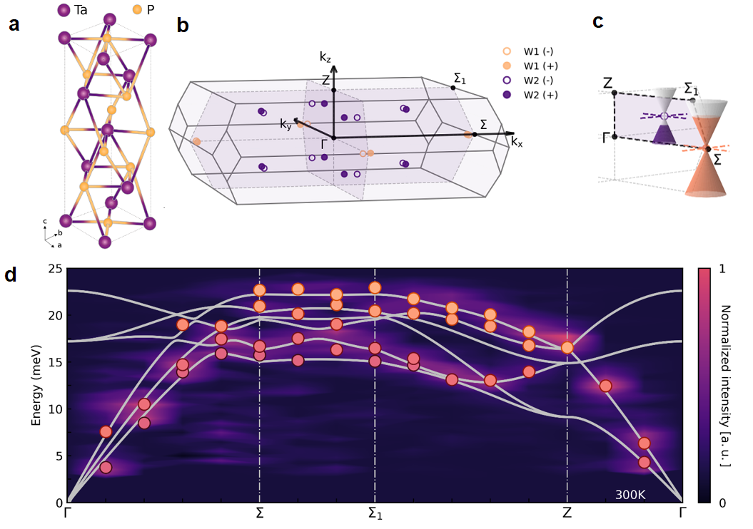
Figure 2: Phonon dispersion of TaP. a. Crystal structure of TaP with b, corresponding Brillouin zone and featuring the locations and Berry curvature signs of paired Weyl nodes W1 (orange) and W2 (purple). c. Schematic of relative energy location of W1 and W2 Weyl nodes. d. Low-energy phonon dispersion of TaP, measured by IXS and INS at 300K along the high-symmetry loop $\Gamma$-$\Sigma$-$\Sigma_{1}$-Z-$\Gamma$. Points represent extracted phonon modes from measurements. The grey lines denote ab initio calculations showing excellent agreement, and the color map represents the spectra intensity.

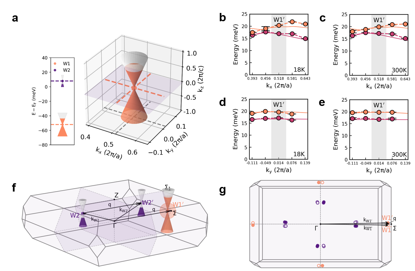
Figure 4: Phonon characteristics at the W1 Weyl node and $\Gamma$-point. a. Location of the W1 Weyl node in energy and momentum space. Dispersions of two representative phonon modes obtained from IXS data near W1 at b, 18K and c, 300K along the $k_{x}$ direction as well as d and e, along the $k_{y}$ direction. Error bars represent one standard deviation. Experimental phonon dispersion agrees excellently with ab initio calculations (solid lines). f. Schematic of the connection of two equivalent electronic states at $\bm{k}_{W2}$ and $\bm{k}_{W2^{\prime}}$ by the phonon $\bm{q}=\bm{k}_{W2^{\prime}}-\bm{k}_{W2}\approx\bm{k}_{W1^{\prime}}$, the W1 node near which IXS measurements were performed. g. Schematic seen from the (001) plane of the connection between two equivalent electronic states at $\bm{k}_{W1^{\prime}}$ and $\bm{k}_{\overline{W1}}$ by the phonon momentum $\bm{q}=\bm{k}_{W1^{\prime}}-\bm{k}_{\overline{W1}}\approx\Gamma$.

Supplementary materials for Topological Singularity Induced Chiral Kohn Anomaly in A Weyl Semimetal

Contents

1. Derivation of polarization and dielectric functions for Weyl semimetals

2. Single crystal growth and sample preparation of TaP for IXS

3. X-ray and neutron scattering measurements and analysis of TaP

4. Computational details

5. Phonon nesting conditions between Weyl nodes in TaP

Supplementary A: Derivation of polarization and dielectric functions for Weyl semimetals

.1 Introduction

In the study of graphene, the dynamical polarization function $\Pi(\nu,\mathbf{q})$ is one of the fundamental quantities required to understand physical properties of the system such as screening due to a charged impurity and the existence of collective excitations such as plasmons. Prior to its investigation in a Weyl semimetal, $\Pi(\nu,\mathbf{q})$ had been extensively studied for graphene. In this section of the paper, we examine in greater detail the dynamical polarization function for a Weyl semimetal which has the possibility of exhibiting topological Fermi arcs on the surface and as well as phenomena such as the chiral magnetic effect in the bulk.

To derive the polarization function $\Pi(\nu,\mathbf{q})$, we will consider a simple continuous model which can be used to describe Weyl semimetals and nodal-line semimetals. Expanding around the $\Gamma$ point, we consider a Hamiltonian in momentum space with tilted Dirac cones as the following

$$\mathcal{H}(\mathbf{k},\mathbf{d})=\hbar v_{F}\left(\mathbf{k}\cdot\sigma+p\mathbf{d}\cdot\mathbf{k}I_{2}\right)-\mu I_{2}$$ (S1)

where $\mathbf{k}=(k_{x},k_{y},k_{z})$ is the momentum and $\sigma=(\sigma_{x},\sigma_{y},\sigma_{z})$ are the Pauli matrices. In addition, $v_{F}$ represents the Fermi velocity, $\mathbf{d}$ is a unit vector, $p$ is a dimensionless parameter which will be referred to as the tilting parameter, and $\mu$ represents the chemical potential. The Hamiltonian above has the following eigenvalues

$$E_{\pm}=\hbar v_{F}(p\mathbf{d}\cdot\mathbf{k}\pm|\mathbf{k}|)-\mu$$ (S2)

Near the band crossing at the Weyl point, the low-energy bands can be linearized in the variation $\mathbf{k}^{\prime}=\mathbf{k}-\mathbf{k}_{Wi}$ of the $\mathbf{k}$ vector with respect to the position $\mathbf{k}_{Wi}$ of the Weyl node $Wi$ which in our case, $i\in\{1,2\}$. Note that the subscript $i$ does not necessarily refer to the subset of inequivalent Weyl nodes as it does in the main text. As such, we can write the Hamiltonian as follows

$$\mathcal{H}(\mathbf{k}^{\prime},\mathbf{d})=\hbar v_{F}\left(\mathbf{k}^{\prime}\cdot\sigma+p\mathbf{d}\cdot\mathbf{k}^{\prime}I_{2}\right)-\mu I_{2}$$ (S3)

with eigenvalues

$$E_{\pm}=\hbar v_{F}(p\mathbf{d}\cdot\mathbf{k}^{\prime}\pm|\mathbf{k}^{\prime}|)-\mu$$ (S4)

The propagator is given by

$$G(i\omega_{n},\mathbf{k}^{\prime},\mathbf{d})=\frac{1}{(i\omega_{n}+\mu-\hbar v_{F}p\mathbf{d}\cdot\mathbf{k}^{\prime})I_{2}-\hbar\nu_{F}\mathbf{k}^{\prime}\cdot\sigma}=\frac{(i\omega_{n}+\mu-\hbar v_{F}p\mathbf{d}\cdot\mathbf{k}^{\prime})I_{2}+\mathbf{k}^{\prime}\cdot\sigma}{(i\omega_{n}+\mu-\hbar v_{F}p\mathbf{d}\cdot\mathbf{k}^{\prime})^{2}-(\hbar v_{F}\mathbf{k}^{\prime})^{2}}$$ (S5)

For convenience, we set the constants $\hbar=v_{F}=1$ during the subsequent intermediate calculations. The relation between plasmons and the polarization function is provided by another important quantity that emerges in solid state physics, the dielectric function $\varepsilon(\nu,\mathbf{q})$, which is given by the relation

$$\varepsilon^{R}(\nu,\mathbf{q})=1-V_{0}(\mathbf{q})\Pi^{R}(\nu,\mathbf{q})$$ (S6)

where $\Pi^{R}(\nu,\mathbf{q})$ is the retarded polarization function and $V_{0}(\mathbf{q})=4\pi e^{2}/\kappa|\mathbf{q}|^{2}$ is the bare Coulomb potential with dielectric constant $\kappa$. For simplicity, we will omit the superscript $R$ used for retarded quantities, i.e., we write for the retarded dielectric function $\varepsilon^{R}(\nu,\mathbf{q})=\varepsilon(\nu,\mathbf{q})$. This notation will also be used for other retarded quantities.

If we consider the inter-Weyl node scattering from the neighborhood of $\mathbf{k}_{W1}$ with the chemical potential $\mu_{1}$ to the neighborhood of $\mathbf{k}_{W2}$ with the chemical potential $\mu_{2}$, as discussed in the main text, the corresponding polarization operator $\Pi(i\nu,\mathbf{q})$ in the Matsubara frequency domain under the random phase approximation can be written as

$$\Pi(i\nu,\mathbf{q})=\frac{1}{\beta}\sum_{n}\int\frac{d^{3}k}{(2\pi)^{3}}\text{Tr}\left[G(i\nu+i\omega_{n}+\mu_{1},\mathbf{q}+\mathbf{k}_{1},\mathbf{d})G(i\omega_{n}+\mu_{2},\mathbf{k}_{2},\mathbf{d})\right]$$ (S7)

with $\mathbf{k}_{1}=\mathbf{k}-\mathbf{k}_{W1}$ and $\mathbf{k}_{2}=\mathbf{k}-\mathbf{k}_{W2}$, respectively.

.2 Derivation of the polarization function for Weyl semimetals

To showcase the results at finite temperature, we return to Eq. (S7). For simplicity we neglect the tilting factor from now on, which is already sufficient to explain the type-I Weyl semimetal behavior. We do the following transformations: $k_{0}=i\omega_{n}+\mu_{2}$, $q_{0}=i\nu+\mu_{1}-\mu_{2}$, $\mathbf{k}^{\prime}=\mathbf{k}-\mathbf{k}_{W2}$, and $\mathbf{q}^{\prime}=\mathbf{q}+\mathbf{k}_{W1}-\mathbf{k}_{W2}$.

$$\Pi(i\nu,\mathbf{q})=\frac{2}{\beta}\sum_{n}\int\frac{d^{3}k^{\prime}}{(2\pi)^{3}}\frac{k_{0}(k_{0}+q_{0})+\mathbf{k}^{\prime}\cdot(\mathbf{k}^{\prime}+\mathbf{q}^{\prime})}{\left((k_{0}+q_{0})^{2}-E_{\mathbf{k}^{\prime}+\mathbf{q}^{\prime}}^{2}\right)\left(k_{0}^{2}-E_{\mathbf{k}^{\prime}}^{2}\right)}$$ (S8)

Afterwards, we perform the summation over Matsubara frequencies according to kapusta_2006:

$$\begin{split}\frac{1}{\beta}\sum_{n}\frac{k_{0}\left(k_{0}+q_{0}\right)+\mathbf{k}^{\prime}\cdot(\mathbf{k}^{\prime}+\mathbf{q}^{\prime})}{(k_{0}^{2}-E_{\mathbf{k}^{\prime}}^{2})\left((k_{0}+q_{0})^{2}-E_{\mathbf{k}^{\prime}+\mathbf{q}^{\prime}}^{2}\right)}=&-\frac{1}{2\pi i}\oint dz\ h(z)g(z)\\ =&-\frac{1}{2\pi i}\left(\int\limits_{i\infty-\delta}^{-i\infty-\delta}dz\ h(z)\frac{1}{2}\tanh\left(\frac{\beta z}{2}\right)+\int\limits_{-i\infty+\delta}^{i\infty+\delta}dz\ h(z)\frac{1}{2}\tanh\left(\frac{\beta z}{2}\right)\right)\\ =&-\frac{1}{2\pi i}\left(\int\limits_{i\infty-\delta}^{-i\infty-\delta}dz\ h(z)\left(\frac{1}{2}-\frac{1}{e^{-\beta z}+1}\right)+\int\limits_{-i\infty+\delta}^{i\infty+\delta}dz\ h(z)\left(-\frac{1}{2}+\frac{1}{e^{\beta z}+1}\right)\right)\end{split}$$

$$h(z) =\frac{(z+\mu_{2})\left(z+\mu_{2}+q_{0}\right)+\mathbf{k}^{\prime}\cdot(\mathbf{k}^{\prime}+\mathbf{q}^{\prime})}{\left((z+\mu_{2})^{2}-E_{\mathbf{k}^{\prime}}^{2}\right)\left(\left(z+\mu_{2}+q_{0}\right)^{2}-E_{\mathbf{k}^{\prime}+\mathbf{q}^{\prime}}^{2}\right)}$$

$$g(z) =\frac{1}{2}\tanh\left(\frac{\beta z}{2}\right)$$

$$E_{\mathbf{k}^{\prime}} =|\mathbf{k}^{\prime}|$$

where the function $g(z)$ has simple poles at $i\omega_{n}$. We can divide the above expression into two parts in order to have two contributions for $\Pi(i\nu,\mathbf{q})$, the vacuum part and the matter part, such that

$$\Pi_{\text{vac}} =-\frac{1}{2\pi i}\int\limits_{-i\infty}^{i\infty}dz\ \frac{1}{2}(h(z)+h(-z))$$ (S9)

$$\Pi_{\text{matter}} =\frac{1}{2\pi i}\int\limits_{-i\infty+\delta}^{i\infty+\delta}dz\ h(z)\frac{1}{e^{\beta z}+1}+\frac{1}{2\pi i}\int\limits_{i\infty-\delta}^{-i\infty-\delta}dz\ h(z)\frac{1}{e^{-\beta z}+1}$$ (S10)

At this point in the derivation, we can simply evaluate the term corresponding to the vacuum part by using $z=i\omega$

$$\begin{split}\Pi_{\text{vac}}(i\nu,\mathbf{q})=&\int\frac{d\omega d^{3}k^{\prime}}{(2\pi)^{4}}\left(\frac{(i\omega+\mu_{2})(i\omega+\mu_{2}+q_{0})+\mathbf{k}^{\prime}\cdot(\mathbf{k}^{\prime}+\mathbf{q}^{\prime})}{((i\omega+\mu_{2}+q_{0})^{2}-|\mathbf{k}^{\prime}+\mathbf{q}^{\prime}|^{2})((i\omega+\mu_{2})^{2}-|\mathbf{k}^{\prime}|^{2})}\right)\\ &+\int\frac{d\omega d^{3}k^{\prime}}{(2\pi)^{4}}\left(\frac{(i\omega+\mu_{2})(i\omega+\mu_{2}-q_{0})+\mathbf{k}^{\prime}\cdot(\mathbf{k}^{\prime}+\mathbf{q}^{\prime})}{((i\omega+\mu_{2}-q_{0})^{2}-|\mathbf{k}^{\prime}+\mathbf{q}^{\prime}|^{2})((i\omega+\mu_{2})^{2}-|\mathbf{k}^{\prime}|^{2})}\right)\\ \approx&-\frac{q^{\prime 2}}{24\pi^{2}}\left(\ln\left(-q_{0}^{2}+q^{\prime 2}+4\Lambda\right)-\ln(-q_{0}^{2}+q^{\prime 2})+\frac{8\Lambda^{3}}{(-q_{0}^{2}+q^{\prime 2})^{3/2}}\text{arctan}\left(\frac{\sqrt{-q_{0}^{2}+q^{\prime 2}}}{2\Lambda}\right)-\frac{4\Lambda^{2}}{-q_{0}^{2}+q^{\prime 2}}\right)\end{split}$$

where we relabeled $k^{\prime}=k$ again, set $q^{\prime}=|\mathbf{q}^{\prime}|$ and omitted the constant terms. We analytically extend the result above into real frequencies by $i\nu\to\nu+i\delta$:

$$\Pi_{\text{vac}}(\nu,\mathbf{q})=-\frac{q^{\prime 2}}{24\pi^{2}}\left(\ln\left(\frac{4\Lambda^{2}+q^{\prime 2}-\nu^{\prime 2}}{q^{\prime 2}-\nu^{\prime 2}}\right)+\frac{8\Lambda^{3}}{(q^{\prime 2}-\nu^{\prime 2})^{3/2}}\text{arctan}\left(\frac{\sqrt{q^{\prime 2}-\nu^{\prime 2}}}{2\Lambda}\right)-\frac{4\Lambda^{2}}{q^{\prime 2}-\nu^{\prime 2}}\right)$$ (S11)

with $\nu^{\prime}=\nu-\mu_{1}+\mu_{2}$. Notice that we have introduced a momentum cutoff $\Lambda$ since the integral over the momentum diverges. Afterwards, we can expand Eq. (S11) in the case that $\Lambda\gg 1$ to obtain:

$$\Pi_{\text{vac}}(\nu,\mathbf{q})\approx-\frac{|\mathbf{q}^{\prime}|^{2}}{24\pi}\left(\ln\left|\frac{4\Lambda^{2}}{|\mathbf{q}^{\prime}|^{2}-\nu^{\prime 2}}\right|+\frac{3(|\mathbf{q}^{\prime}|^{2}-\nu^{\prime 2})}{10\Lambda^{2}}-\frac{1}{3}\right)$$ (S12)

In order to obtain the real and imaginary parts of $\Pi_{vac}$, we can use the generalized Kramers-Kronig relation bjorken_1966.

$$\begin{split}\text{Re}[\Pi_{\text{vac}}(\nu,\mathbf{q})]=\text{Re}[\Pi_{\text{vac}}(0,\mathbf{q})]+\frac{E}{\pi}\mathcal{P}\int_{-\infty}^{\infty}d\omega\frac{\text{Im}[\Pi_{\text{vac}}(\nu,\mathbf{q})]}{\omega(\omega-E)}\\ \text{Im}[\Pi_{\text{vac}}(\nu,\mathbf{q})]=\text{Im}[\Pi_{\text{vac}}(0,\mathbf{q})]-\frac{E}{\pi}\mathcal{P}\int_{-\infty}^{\infty}d\omega\frac{\text{Re}[\Pi_{\text{vac}}(\nu,\mathbf{q})]}{\omega(\omega-E)}\end{split}$$ (S13)

Therefore, $\Pi_{\text{vac}}$ is given by

$$\Pi_{\text{vac}}(\nu,\mathbf{q})=-\frac{q^{\prime 2}}{24\pi^{2}}\left(\ln\left|\frac{4\Lambda^{2}+q^{\prime 2}-\nu^{\prime 2}}{q^{\prime 2}-\nu^{\prime 2}}\right|+\frac{8\Lambda^{3}}{(q^{\prime 2}-\nu^{\prime 2})^{3/2}}\text{arctan}\left(\frac{\sqrt{q^{\prime 2}-\nu^{\prime 2}}}{2\Lambda}\right)-\frac{4\Lambda^{2}}{q^{\prime 2}-\nu^{\prime 2}}+i\pi\Theta(\nu^{\prime}-q^{\prime})\right)$$ (S14)

where we have considered $\text{Im}[\Pi_{\text{vac}}(0,\mathbf{q})]=0$. The imaginary part of $\Pi_{\text{vac}}(\nu,\mathbf{q})$ is given by

$$\text{Im}[\Pi_{\text{vac}}(\nu,\mathbf{q})]=-\Theta(\nu^{\prime}-q^{\prime})\frac{q^{\prime 2}}{24\pi}$$ (S15)

The real part of Eq. (S14) is given by

$$\text{Re}[\Pi_{\text{vac}}(\nu,\mathbf{q})]=-\frac{q^{\prime 2}}{24\pi^{2}}\left(\ln\left|\frac{4\Lambda^{2}+q^{\prime 2}-\nu^{\prime 2}}{q^{\prime 2}-\nu^{\prime 2}}\right|+\frac{8\Lambda^{3}}{(q^{\prime 2}-\nu^{\prime 2})^{3/2}}\text{arctan}\left(\frac{\sqrt{q^{\prime 2}-\nu^{\prime 2}}}{2\Lambda}\right)-\frac{4\Lambda^{2}}{q^{\prime 2}-\nu^{\prime 2}}\right)$$ (S16)

We see that the logarithm always carries an imaginary part since its argument is negative. Let us evaluate the matter component of the polarization function.

$$\Pi_{\text{matter}}= \frac{1}{2\pi i}\int\limits_{-i\infty+\delta}^{i\infty+\delta}dz\ h(z)\frac{1}{e^{\beta z}+1}+\frac{1}{2\pi i}\int\limits_{i\infty-\delta}^{-i\infty-\delta}dz\ h(z)\frac{1}{e^{-\beta z}+1}$$

$$= \ \frac{1}{2E_{\mathbf{k}^{\prime}}}\left(\frac{E_{\mathbf{k}^{\prime}}\left(E_{\mathbf{k}^{\prime}}+q_{0}\right)+\mathbf{k}^{\prime}\cdot(\mathbf{k}^{\prime}+\mathbf{q}^{\prime})}{\left(E_{\mathbf{k}^{\prime}}+q_{0}\right)^{2}-E_{\mathbf{k}^{\prime}+\mathbf{q}^{\prime}}^{2}}\right)\frac{1}{e^{\beta\left(E_{\mathbf{k}^{\prime}}+\mu_{2}\right)}+1}$$

$$+\frac{1}{2E_{\mathbf{k}^{\prime}}}\left(\frac{E_{\mathbf{k}^{\prime}}\left(E_{\mathbf{k}^{\prime}}-q_{0}\right)+\mathbf{k}^{\prime}\cdot(\mathbf{k}^{\prime}+\mathbf{q}^{\prime})}{\left(E_{\mathbf{k}^{\prime}}-q_{0}\right)^{2}-E_{\mathbf{k}^{\prime}+\mathbf{q}^{\prime}}^{2}}\right)\frac{1}{e^{\beta\left(E_{\mathbf{k}^{\prime}}-\mu_{2}\right)}+1}$$

$$+\frac{1}{2E_{\mathbf{k}^{\prime}+\mathbf{q}^{\prime}}}\left(\frac{E_{\mathbf{k}^{\prime}+\mathbf{q}^{\prime}}\left(E_{\mathbf{k}^{\prime}+\mathbf{q}^{\prime}}+q_{0}\right)+\mathbf{k}^{\prime}\cdot(\mathbf{k}^{\prime}+\mathbf{q}^{\prime})}{\left(E_{\mathbf{k}^{\prime}+\mathbf{q}^{\prime}}+q_{0}\right)^{2}-E_{\mathbf{k}^{\prime}}^{2}}\right)\frac{1}{e^{\beta\left(E_{\mathbf{k}^{\prime}+\mathbf{q}^{\prime}}-\mu_{1}\right)}+1}$$

$$+\frac{1}{2E_{\mathbf{k}^{\prime}+\mathbf{q}^{\prime}}}\left(\frac{E_{\mathbf{k}^{\prime}+\mathbf{q}^{\prime}}\left(E_{\mathbf{k}^{\prime}+\mathbf{q}^{\prime}}-q_{0}\right)+\mathbf{k}^{\prime}\cdot(\mathbf{k}^{\prime}+\mathbf{q}^{\prime})}{\left(E_{\mathbf{k}^{\prime}+\mathbf{q}^{\prime}}-q_{0}\right)^{2}-E_{\mathbf{k}^{\prime}}^{2}}\right)\frac{1}{e^{\beta\left(E_{\mathbf{k}^{\prime}+\mathbf{q}^{\prime}}+\mu_{1}\right)+1}}$$

$$= \ \frac{1}{2E_{\mathbf{k^{\prime}}}}\sum_{s=\pm}f^{s}\left(q_{0}\right)N_{F}^{s}\left(E_{\mathbf{k}^{\prime}}\right)$$

$$f^{s}\left(q_{0}\right) =\frac{E_{\mathbf{k}^{\prime}}\left(E_{\mathbf{k}^{\prime}}+sq_{0}\right)+\mathbf{k}\cdot(\mathbf{k}^{\prime}+\mathbf{q}^{\prime})}{\left(E_{\mathbf{k}^{\prime}}+sq_{0}\right)^{2}-E_{\mathbf{k}^{\prime}+\mathbf{q}^{\prime}}^{2}}$$ (S17)

$$N_{F}^{s}\left(E_{\mathbf{k}^{\prime}}\right) =\frac{1}{e^{\beta\left(E_{\mathbf{k}^{\prime}}-s\mu_{1}\right)}+1}+\frac{1}{e^{\beta\left(E_{\mathbf{k}^{\prime}}+s\mu_{2}\right)}+1}$$ (S18)

where we considered the following change of variable: $\mathbf{k}^{\prime}\to-\mathbf{k}^{\prime}-\mathbf{q}^{\prime}$. If we take into account the finite density effect, the Fermi energy could lie either in the valence band ($\mu_{1}$, $\mu_{2}<0$) or in the conduction band ($\mu_{1}$, $\mu_{2}>0$).

$$\Pi_{\text{matter}}(\nu,\mathbf{q},T) =2\int\frac{d^{3}k^{\prime}}{(2\pi)^{3}}\frac{1}{2E_{\mathbf{k}^{\prime}}}\sum_{s=\pm}f^{s}(q_{0})N_{F}^{s}\left(E_{\mathbf{k}^{\prime}}\right)$$

$$=\frac{1}{8\pi^{3}}\int\limits_{0}^{\infty}dk^{\prime}\int\limits_{0}^{2\pi}d\phi\int\limits_{0}^{\pi}d\theta\sum_{s=\pm}k^{2}\sin\theta\frac{s(\nu+\mu_{1}-\mu_{2}+i\delta)+2k^{\prime}+q^{\prime}\cos\theta}{(\nu+\mu_{1}-\mu_{2}+i\delta+s|k^{\prime}|)^{2}-(k^{\prime 2}+q^{\prime 2}+2k^{\prime}q^{\prime}\cos\theta)}N_{F}^{s}(|k^{\prime}|)$$

We can obtain the real part of $\Pi_{\text{matter}}(\nu,\mathbf{q},T)$

$$\text{Re}[\Pi_{\text{matter}}(\nu,\mathbf{q},T)]=\frac{1}{8\pi^{3}}\int_{0}^{\infty}dk^{\prime}\sum_{s=\pm}J^{s}(\nu,\mathbf{k}^{\prime},\mathbf{q}^{\prime},T)$$ (S19)

$$J^{s}(\nu,\mathbf{k}^{\prime},\mathbf{q}^{\prime},T)=-2\pi k^{\prime}N_{F}^{s}(|k^{\prime}|)-\pi\frac{(2sk^{\prime}+\nu^{\prime})^{2}-q^{\prime 2}}{2q^{\prime}}N_{F}^{s}(|k^{\prime}|)\ln\left|\frac{(q^{\prime}-s\nu^{\prime})(2k^{\prime}+s\nu+q^{\prime})}{(s\nu^{\prime}+q^{\prime})(q^{\prime}-2k^{\prime}-s\nu^{\prime})}\right|$$ (S20)

At nonzero temperatures, the momentum space integral cannot be evaluated analytically. Therefore, we initially compute the polarization function at zero temperature in which an analytic treatment is adequate. The zero temperature scenario, despite being simple, still exhibits the Kohn anomaly observed in experiment.

.3 Zero temperature results

At zero temperature, $N_{F}^{s}(E_{\mathbf{k}^{\prime}})$ can be replaced by the Heaviside step functions as the following

$$\lim_{\beta\to\infty}N_{F}^{s}(E_{\mathbf{k}^{\prime}})=\Theta(s\mu_{1}-E_{\mathbf{k^{\prime}}})+\Theta(-s\mu_{2}-E_{\mathbf{k^{\prime}}})$$ (S21)

Hereafter, we consider only the absolute values of the chemical potentials $|\mu_{1}|$ and $|\mu_{2}|$ and we only present results for $\mu_{1}$, $\mu_{2}>0$. Thus, at zero temperature, we obtain

$$\textrm{Re}[\Pi_{\text{matter}}(\nu,\mathbf{q},T=0)]= \ -\frac{1}{6\pi^{2}}(\mu_{1}^{2}+\mu_{2}^{2})-\frac{1}{24\pi^{2}}\nu^{\prime}(\mu_{1}-\mu_{2})$$

$$+\frac{q^{\prime 2}}{32\pi^{2}}\sum_{s=\pm 1}g_{3}\left(\frac{2\mu_{1}+\nu^{\prime}}{sq^{\prime}}\right)\ln\left|\frac{2\mu_{1}+\nu^{\prime}-sq^{\prime}}{\nu^{\prime}-sq^{\prime}}\right|$$

$$+\frac{q^{\prime 2}}{32\pi^{2}}\sum_{s=\pm 1}g_{3}\left(\frac{2\mu_{2}-\nu^{\prime}}{sq^{\prime}}\right)\ln\left|\frac{2\mu_{2}-\nu^{\prime}-sq^{\prime}}{\nu^{\prime}+sq^{\prime}}\right|$$

where

$$g_{3}(x)=x\left(\frac{x^{2}}{3}-1\right)+\frac{2}{3}\qquad\nu^{\prime}=\nu-\mu_{1}+\mu_{2}$$

The zero-temperature results are consistent with recent calculations lv_2013; zhou_2015; thakur_2018; sadhukhan_2020. Adding the vacuum and the matter parts together, we obtain the real part of the polarization function at zero temperature

$$\begin{split}\operatorname{Re}[\Pi(\nu,\mathbf{q},T=0)]=&\frac{q^{\prime 2}}{32\pi^{2}}\sum_{s=\pm 1}g_{3}\left(\frac{2\mu_{1}+\nu^{\prime}}{sq^{\prime}}\right)\ln\left|\frac{2\mu_{1}+\nu^{\prime}-sq^{\prime}}{\nu^{\prime}-sq^{\prime}}\right|+\frac{q^{\prime 2}}{32\pi^{2}}\sum_{s=\pm 1}g_{3}\left(\frac{2\mu_{2}-\nu^{\prime}}{sq^{\prime}}\right)\ln\left|\frac{2\mu_{2}-\nu^{\prime}-sq^{\prime}}{\nu^{\prime}+sq^{\prime}}\right|\\ &-\frac{1}{6\pi^{2}}(\mu_{1}^{2}+\mu_{2}^{2})-\frac{1}{24\pi^{2}}(\nu^{\prime}\mu_{1}-\nu^{\prime}\mu_{2})-\frac{q^{\prime 2}}{24\pi^{2}}\left(\ln\left|\frac{4\Lambda^{2}}{q^{\prime 2}-\nu^{\prime 2}}\right|-\frac{1}{3}+\frac{3(q^{\prime 2}-\nu^{\prime 2})}{10\Lambda^{2}}\right)\end{split}$$ (S22)

Now, we calculate the imaginary part of the polarization function for the matter term using $\Theta=\frac{\mathbf{k^{\prime}}\cdot(\mathbf{k^{\prime}+q^{\prime}})}{|\mathbf{k^{\prime}}||\mathbf{k^{\prime}+q^{\prime}}|}$ to obtain

$$\text{Im}[\Pi_{\text{matter}}(\nu,\mathbf{q},T)]= \int\frac{d^{3}k^{\prime}}{(2\pi)^{3}}\frac{(\nu+\mu_{1}-\mu_{2}+i\delta)+|\mathbf{k^{\prime}}|+|\mathbf{k^{\prime}+q^{\prime}}|\cos\Theta}{(\nu+\mu_{1}-\mu_{2}+i\delta+|\mathbf{k^{\prime}}|)^{2}-|\mathbf{k^{\prime}+q^{\prime}}|^{2}}N_{F}^{+}(|\mathbf{k^{\prime}}|)$$

$$-\int\frac{d^{3}k^{\prime}}{(2\pi)^{3}}\frac{(\nu+\mu_{1}-\mu_{2}+i\delta)-|\mathbf{k^{\prime}}|-|\mathbf{k^{\prime}+q^{\prime}}|\cos\Theta}{(\nu+\mu_{1}-\mu_{2}+i\delta-|\mathbf{k^{\prime}}|)^{2}-|\mathbf{k^{\prime}+q^{\prime}}|^{2}}N_{F}^{-}(|\mathbf{k^{\prime}}|)$$

$$= \ \text{Im}[\Pi_{\text{matter}}^{+}(\nu,\mathbf{q},T)]+\text{Im}[\Pi_{\text{matter}}^{-}(\nu,\mathbf{q},T)]$$

with the following terms

$$\text{Im}[\Pi_{\text{matter}}^{+}(\nu,\mathbf{q},T)]= \ -\frac{\Theta(q^{\prime}-\nu^{\prime})}{16\pi}\Theta(q^{\prime}+\nu^{\prime})\int\limits_{\frac{q^{\prime}-\nu^{\prime}}{2}}^{\infty}dk^{\prime}N_{F}^{+}(k^{\prime})\frac{(2k^{\prime}+\nu^{\prime})^{2}-q^{\prime 2}}{q^{\prime}}$$

$$-\frac{\Theta(-q^{\prime}-\nu^{\prime})}{16\pi}\Theta(q^{\prime}-\nu^{\prime})\int_{0}^{\infty}dk^{\prime}N_{F}^{+}(k^{\prime})\frac{(2k^{\prime}+\nu^{\prime})^{2}-q^{\prime 2}}{q^{\prime}}\left[\Theta\left(\frac{q^{\prime}-\nu^{\prime}}{2}-k^{\prime}\right)-\Theta\left(\frac{-\nu^{\prime}-q^{\prime}}{2}-k^{\prime}\right)\right]$$

$$\text{Im}[\Pi_{\text{matter}}^{-}(\nu,\mathbf{q},T)]= +\frac{\Theta(q^{\prime}+\nu^{\prime})}{16\pi}\Theta(q^{\prime}-\nu^{\prime})\int\limits_{\frac{q^{\prime}+\nu^{\prime}}{2}}^{\infty}dk^{\prime}N_{F}^{-}(k^{\prime})\frac{(-2k^{\prime}+\nu^{\prime})^{2}-q^{\prime 2}}{q^{\prime}}$$

$$-\frac{\Theta(q^{\prime}+\nu^{\prime})}{16\pi}\Theta(\nu^{\prime}-q^{\prime})\int_{0}^{\infty}dk^{\prime}N_{F}^{-}(k^{\prime})\frac{(-2k^{\prime}+\nu^{\prime})^{2}-q^{\prime 2}}{q^{\prime}}\left[\Theta\left(\frac{q^{\prime}+\nu^{\prime}}{2}-k^{\prime}\right)-\Theta\left(\frac{\nu^{\prime}-q^{\prime}}{2}-k^{\prime}\right)\right]$$

Combining the vacuum and matter parts, we obtain the imaginary part of $\Pi(\nu,\mathbf{q},T=0)$ at zero temperature as follows

$$\begin{split}\text{Im}[\Pi(\nu,\mathbf{q},T=0)]=\enskip&-\frac{q^{\prime 2}}{24\pi}\Theta(\nu^{\prime}-q^{\prime})\\ &-\frac{q^{\prime 2}}{32\pi}\Theta(q^{\prime}-\nu^{\prime})\Theta(q^{\prime}+\nu^{\prime})\Theta\left(\frac{2\mu_{1}+\nu^{\prime}}{q^{\prime}}-1\right)g_{3}\left(\frac{2\mu_{1}+\nu^{\prime}}{q^{\prime}}\right)\\ &-\frac{q^{\prime 2}}{32\pi}\Theta(-q^{\prime}-\nu^{\prime})\Theta(q^{\prime}-\nu^{\prime})\Theta\left(1-\frac{2\mu_{1}+\nu^{\prime}}{q^{\prime}}\right)g_{3}\left(\frac{2\mu_{1}+\nu^{\prime}}{q^{\prime}}\right)\\ &+\frac{q^{\prime 2}}{32\pi}\Theta(-q^{\prime}-\nu^{\prime})\Theta(q^{\prime}-\nu^{\prime})\Theta\left(-1-\frac{2\mu_{1}+\nu^{\prime}}{q^{\prime}}\right)g_{3}\left(\frac{2\mu_{1}+\nu^{\prime}}{q^{\prime}}\right)\\ &+\frac{q^{\prime 2}}{24\pi}\Theta(-q^{\prime}-\nu^{\prime})\Theta(q^{\prime}-\nu^{\prime})\Theta\left(\frac{2\mu_{1}+\nu^{\prime}}{q^{\prime}}+1\right)\\ &+\frac{q^{\prime 2}}{32\pi}\Theta(q^{\prime}+\nu^{\prime})\Theta(q^{\prime}-\nu^{\prime})\Theta\left(\frac{2\mu_{2}-\nu^{\prime}}{q^{\prime}}-1\right)g_{3}\left(\frac{2\mu_{2}-\nu^{\prime}}{q^{\prime}}\right)\\ &-\frac{q^{\prime 2}}{32\pi}\Theta(\nu^{\prime}-q^{\prime})\Theta(q^{\prime}+\nu^{\prime})\Theta\left(1-\frac{2\mu_{2}-\nu^{\prime}}{q^{\prime}}\right)g_{3}\left(\frac{2\mu_{2}-\nu^{\prime}}{q^{\prime}}\right)\\ &+\frac{q^{\prime 2}}{32\pi}\Theta(\nu^{\prime}-q^{\prime})\Theta(q^{\prime}+\nu^{\prime})\Theta\left(-1-\frac{2\mu_{2}-\nu^{\prime}}{q^{\prime}}\right)g_{3}\left(\frac{2\mu_{2}-\nu^{\prime}}{q^{\prime}}\right)\\ &+\frac{q^{\prime 2}}{24\pi}\Theta(\nu^{\prime}-q^{\prime})\Theta(q^{\prime}+\nu^{\prime})\Theta\left(\frac{2\mu_{2}-\nu^{\prime}}{q^{\prime}}+1\right)\end{split}$$ (S23)

.4 Kohn anomaly from singularities of the polarization function $\Pi(\nu,\textbf{q})$

The Kohn anomaly is an anomaly in the dispersion relation and describes a sudden dip in frequency for a particular wavevector. The phonon dispersion relation is given by

$$\omega_{\mathbf{q}}^{2}=\frac{\Omega_{\mathbf{q}}^{2}}{\varepsilon(\nu,\mathbf{q})}\qquad\varepsilon(\nu,\mathbf{q})=1-V_{0}(\mathbf{q})\text{Re}[\Pi(\nu,\mathbf{q})]$$ (S24)

where $\omega_{\mathbf{q}}$ and $\Omega_{\mathbf{q}}$ are the renormalized phonon frequency due to electronic RPA screening and the bare phonon frequency, respectively. The subscript $r$ means the designates part. Thus, in order to find the Kohn anomaly, we must study the singularities of $\Pi(\nu,\mathbf{q})$.

One might naively think that $\operatorname{Re}[\Pi(\nu,\mathbf{q})]$ has poles at $q^{\prime}=|\nu^{\prime}|$, $q^{\prime}=|2\mu_{1}+\nu^{\prime}|$ and $q^{\prime}=|2\mu_{2}-\nu^{\prime}|$. However, upon closer inspection, this guess turns out to be only partly correct. In the case $q^{\prime}=|2\mu_{1}+\nu^{\prime}|$ , observe from Eq. (S22) that the apparently divergent term is of the form

$$x\to 0:g_{3}(1+x)\ln{|x|}\sim x^{2}\ln{|x|}=0\qquad x\equiv\frac{|2\mu_{1}+\nu^{\prime}|}{q^{\prime}}-1$$ (S25)

and therefore vanishes. This is consistent with the fact that $\operatorname{Im}[\Pi(\nu,\mathbf{q})]$ is continuous and well defined at $q^{\prime}=|2\mu_{1}+\nu^{\prime}|$. Similarly, the alleged pole at $q^{\prime}=|2\mu_{2}-\nu^{\prime}|$ disappears upon closer scrutiny.

For the case $q^{\prime}\to|\nu^{\prime}|$, by taking the most divergent terms, we see from Eq. (S22) that

$$\operatorname{Re}[\Pi(\nu,\mathbf{q})]\simeq\frac{q^{\prime 2}}{32\pi^{2}}\left(g_{3}\left(1+\frac{2\mu_{1}}{\nu^{\prime}}\right)\ln\left|\frac{2\mu_{1}}{q^{\prime}-|\nu^{\prime}|}\right|+g_{3}\left(1-\frac{2\mu_{2}}{\nu^{\prime}}\right)\ln\left|\frac{2\mu_{2}}{q^{\prime}-|\nu^{\prime}|}\right|\right)-\frac{q^{\prime 2}}{24\pi^{2}}\ln{\left|\frac{4\Lambda^{2}}{q^{\prime 2}-\nu^{\prime 2}}\right|}\to\infty$$ (S26)

This divergence of $\operatorname{Re}[\Pi(\nu,\mathbf{q})]$ goes hand in hand with the discontinuity of $\operatorname{Im}[\Pi(\nu,\mathbf{q})]$ at $q^{\prime}=|\nu^{\prime}|$.

$$\frac{\partial}{\partial q^{\prime}}\operatorname{Re}[\Pi(\nu,\mathbf{q})]\simeq \frac{q^{\prime}}{16\pi^{2}}\left(g_{3}\left(1+\frac{2\mu_{1}}{\nu^{\prime}}\right)\ln\left|\frac{2\mu_{1}}{q^{\prime}-|\nu^{\prime}|}\right|+g_{3}\left(1-\frac{2\mu_{2}}{\nu^{\prime}}\right)\ln\left|\frac{2\mu_{2}}{q^{\prime}-|\nu^{\prime}|}\right|\right)-\frac{q^{\prime}}{12\pi^{2}}\ln{\left|\frac{4\Lambda^{2}}{q^{\prime 2}-\nu^{\prime 2}}\right|}$$ (S27)

$$-\frac{q^{\prime 2}}{32\pi^{2}}\left(g_{3}\left(1+\frac{2\mu_{1}}{\nu^{\prime}}\right)\frac{1}{q^{\prime}-|\nu^{\prime}|}+g_{3}\left(1-\frac{2\mu_{2}}{\nu^{\prime}}\right)\frac{1}{q^{\prime}-|\nu^{\prime}|}\right)+\frac{1}{12\pi^{2}}\frac{q^{\prime 3}}{q^{\prime 2}-\nu^{\prime 2}}$$

The derivative of the real part of the dielectric function is

$$\frac{\partial\varepsilon}{\partial q}=-2V_{0}(\mathbf{q})\text{Re}[\Pi(\nu,\mathbf{q})]\left(\frac{1}{q^{\prime}}-\frac{1}{q}\right)-V_{0}(\mathbf{q})\frac{\partial}{\partial q^{\prime}}\text{Re}[\Pi(\nu,\mathbf{q})]$$ (S28)

The first term is logarithmically divergent from Eq. (S26) and the second term includes both the logarithmic and power-law divergence. By only including the power-law divergence, which diverges faster than the logarithmic divergence, we find in the limit $q^{\prime}\rightarrow|\nu^{\prime}|$

$$\frac{\partial\varepsilon}{\partial q}\propto-V_{0}(\mathbf{q})\left(\frac{q^{\prime 2}}{32\pi^{2}}\left(g_{3}\left(1+\frac{2\mu_{1}}{\nu^{\prime}}\right)\frac{1}{q^{\prime}-|\nu^{\prime}|}+g_{3}\left(1-\frac{2\mu_{2}}{\nu^{\prime}}\right)\frac{1}{q^{\prime}-|\nu^{\prime}|}\right)+\frac{1}{12\pi^{2}}\frac{q^{\prime 3}}{q^{\prime 2}-\nu^{\prime 2}}\right)$$ (S29)

Therefore, we observe a Kohn anomaly at $q^{\prime}=|\nu^{\prime}|=|\nu-\mu_{1}+\mu_{2}|$, where the polarization function blows up. Notice that the location of the pole only depends on the difference between the chemical potentials of the two nodes.

.5 Finite temperature results

In the following section, we take into account the finite temperature-dependence of the polarization. The real part of the polarization function at $T>0$ is

$$\begin{split}\text{Re}[\Pi(\nu,\mathbf{q},T)]=&-\frac{q^{\prime 2}}{24\pi^{2}}\left(\ln\left|\frac{4\Lambda^{2}}{q^{\prime 2}-\nu^{\prime 2}}\right|+\frac{3(q^{\prime 2}-\nu^{\prime 2})-\frac{1}{3}}{10\Lambda^{2}}\right)+\frac{\Gamma(2)}{4\pi^{2}}\sum_{s=\pm}\frac{1}{\beta^{2}}\left[\text{Li}_{2}\left(-e^{s\beta\mu_{1}}\right)+\text{Li}_{2}\left(-e^{-s\beta\mu_{2}}\right)\right]\\ &-\frac{1}{32\pi^{2}}\left(\frac{\nu^{\prime}}{q^{\prime}}F_{+}(\nu,q,T)+\frac{\nu^{\prime}}{q^{\prime}}F_{-}(\nu,q,T)\right)\end{split}$$ (S30)

with

$$F_{\pm}(\nu,q,T)=\int\limits_{\pm 1}^{\infty}du\left(\frac{(\nu^{\prime}u)^{2}-(q^{\prime})^{2}}{\text{exp}\left(\frac{(\nu^{\prime}u\mp\nu^{\prime})\pm 2\mu_{2}}{2k_{B}T}\right)+1}+\frac{(\nu^{\prime}u)^{2}-(q^{\prime})^{2}}{\text{exp}\left(\frac{(\nu^{\prime}u\mp\nu^{\prime})\mp 2\mu_{1}}{2k_{B}T}\right)+1}\right)\ln\left|\frac{(\pm\nu^{\prime}-q^{\prime})(\nu^{\prime}u+q^{\prime})}{(\pm\nu^{\prime}+q^{\prime})(\nu^{\prime}u-q^{\prime})}\right|$$ (S31)

The imaginary part of the polarization function at finite temperatures $T>0$ can be expressed as

$$\begin{split}\text{Im}[\Pi(\nu,\mathbf{q},T)]=&\ -\frac{q^{\prime 2}}{32\pi}\Theta(q^{\prime}+\nu^{\prime})\left(\Theta(q^{\prime}-\nu^{\prime})\left(G_{+}(\nu,\mathbf{q},T)+G_{-}(\nu,\mathbf{q},T)\right)-\Theta(\nu^{\prime}-q^{\prime})H(\nu,\mathbf{q},T)\right)\\ &-\frac{q^{\prime 2}}{24\pi}\Theta(\nu^{\prime}-q^{\prime})-\frac{q^{\prime 2}}{32\pi^{2}}\Theta(-q^{\prime}-\nu^{\prime})\Theta(q^{\prime}-\nu^{\prime})M(\nu,q,T)\end{split}$$ (S32)

$$G_{\pm}(\nu,\mathbf{q},T)=\int\limits_{1}^{\infty}du\left(\frac{u^{2}-1}{\text{exp}\left(\frac{(q^{\prime}u\mp\nu^{\prime})\pm 2\mu_{2}}{2k_{B}T}\right)+1}+\frac{u^{2}-1}{\text{exp}\left(\frac{(q^{\prime}u\mp\nu^{\prime})\mp 2\mu_{1}}{2k_{B}T}\right)+1}\right)$$ (S33)

$$H(\nu,\mathbf{q},T)=\int\limits_{-1}^{1}du\left(\frac{u^{2}-1}{\text{exp}\left(\frac{(q^{\prime}u+\nu^{\prime})-2\mu_{2}}{2k_{B}T}\right)+1}+\frac{u^{2}-1}{\text{exp}\left(\frac{(q^{\prime}u+\nu^{\prime})+2\mu_{1}}{2k_{B}T}\right)+1}\right)$$ (S34)

$$M(\nu,q,T)=\int\limits_{-1}^{1}du\left(\frac{u^{2}-1}{\text{exp}\left(\frac{(q^{\prime}u-\nu^{\prime})+2\mu_{2}}{2k_{B}T}\right)+1}+\frac{u^{2}-1}{\text{exp}\left(\frac{(q^{\prime}u-\nu^{\prime})-2\mu_{1}}{2k_{B}T}\right)+1}\right)$$ (S35)

While for finite temperatures, exact analytic expressions cannot easily be obtained, it is possible to obtain numerical results from our semi-analytical results.

Supplementary B: Single crystal growth and sample preparation of TaP for IXS

Single crystals of tantalum phosphide (TaP) were prepared using the chemical vapor transport method. 3g of Ta (Beantown Chemical, 99.95%) and P (Beantown Chemical, 99.999%) powders were weighed and mixed together inside a glovebox. They were subsequently flame-sealed inside a quartz tube and then heated to 70^∘C to be held for 20 hours before a pre-reaction. Afterwards, the obtained TaP powder was sealed inside another quartz tube with 0.4g of I₂ (Sigma Aldrich, $\geq$ 99.8%) and this tube was horizontally placed in a two-zone furnace. To improve the crystal size and quality, instead of setting a 100^∘C temperature difference, we gradually increased the temperature difference from zero until the point the I₂ transport agent started to flow. This process seems to be furnace- and distance-specific. In our case, the optimal temperatures for the two zones were 900^∘C and 950^∘C, respectively, and the distance between the two heating zones was constantly optimized. With the help of the transport agent I₂, the TaP source materials were transferred from the cold end of the tube to the hot end and condensed into single-crystalline form within 14 days. The single crystals are centimeter-sized and have a metallic luster (Figure S3). The Fermi level information of this sample is well-characterized in a separate study han_2019.

Due to the high X-ray absorption of tantalum and the large c-axis dimension of the crystals grown in laboratory, the thickness of the samples were required to be reduced to a suitable value for performing inelastic x-ray scattering (IXS) experiments. We determined that the optimal sample thickness for our experiment configuration corresponding to an X-ray wavelength of 0.5725Å was $\sim$20$\mu$m, allowing for a photon transmission of 0.33. A portion of the crystal had its orientation determined using a back-scattering Laue diffractometer and afterwards, it was thinned down to $\sim$20$\mu$m by polishing followed by being glued onto a brass sample holder with a GE-vanish (as the other end of the sample holder was connected to the cryostat). Figure S1 shows top and side views of the orientated thinned-down sample used for our IXS experiments.

Supplementary C: X-ray and neutron scattering measurements and analysis of TaP

Inelastic X-ray scattering experiments. Inelastic X-ray scattering measurements were performed on the high-energy resolution inelastic X-ray (HERIX) instrument at sector 3-ID beamline of the Advanced Photon Source, Argonne National Laboratory, with incident beam energy of 21.657keV ($\lambda=0.5725$Å) and overall energy resolution of 2.1meV sinn_2001; alatas_2011; toellner_2011. The incident beam was focused on the sample using a toroidal and KB mirror system. The full width at half maximum (FWHM) of the beam size at sample position was 20x20$\mu$m² (V$\times$H). The spectrometer was functioning in the horizontal scattering geometry with horizontally polarized radiation. The scattered beam was analyzed by diced and spherically curved silicon (18 6 0) analyzers working at the backscattering angle. The measurements were performed at temperatures of 18K, 60K, 100K and 300K.

Inelastic neutron scattering experiments. Inelastic neutron scattering (INS) was performed at the HB1 polarized triple-axis spectrometer at the High-Flux Isotope Reactor at the Oak Ridge National Laboratory. We used a fixed $E_{f}=14.7$meV with 48${}^{\prime}-$40${}^{\prime}-$40${}^{\prime}-$120^′ collimation and Pyrolytic Graphite filters to eliminate higher-harmonic neutrons. Measurements were performed using closed-cycle refrigerators between room temperature and the base temperature of 4K. INS measurements were also performed at the BT-7 double focusing triple-axis spectrometer lynn_2012 at the NIST Center for Neutron Research at the National Institute of Standards and Technology. At this research facility, we used the same fixed final energy with an open$-$80${}^{\prime}-$80${}^{\prime}-$120^′ collimation and Pyrolytic Graphite filters. Measurements were performed at 10K.

Analysis of IXS and INS experimental data. Statistical error is taken to be square root of the number of counts from Poisson statistics. Repeated IXS scans were performed for certain $\bm{q}$ points and subsequently merged together to reduce statistical noise. Spectra obtained from constant wavevector IXS scans (measuring intensity of counts versus energy transfer) were normalized by area and fitted using a fitting core function of damped harmonic oscillators that were convoluted with a pseudo-Voigt function representing the instrument resolution function, measured before the experiment took place. The number of Lorentzian peaks, corresponding to the number of phonon modes, added to the fitting core was known from ab initio phonon dispersion calculations within the measured energy range. Each fitted peak has parameters corresponding to center, FWHM and amplitude. The latter was furthermore modulated during the fit to take into account the longitudinal and transversal modes of propagation with respect to the scan direction. In our case, due to the inadequate energy resolution necessary for a precise FWHM measurement, more care was taken into the fit to extract accurate peak center locations, corresponding to the energy of the phonon mode. Plots of the phonon dispersion shown in Figures 2f and S6 are created by plotting the fitted core after deconvolution with the instrumental resolution function. The INS scans were treated in an analogous manner by using the Data Analysis and Visualization Environment (dave) software dave_2009 and neutronpy based on the ResLib program package. The resolution function was calculated with knowledge of the monochromator and analyzer crystals, the collimation as well as the sample configuration of our experiment in neutronpy. The phonon modes were modeled using Lorentzian functions as was done for IXS. For the INS data, the intensity near the elastic peak was difficult to resolve for phonon modes located near this energy transfer due to poorer energy resolution and were therefore neglected in favor of extracting phonon modes with larger energy transfer with these INS data scans.

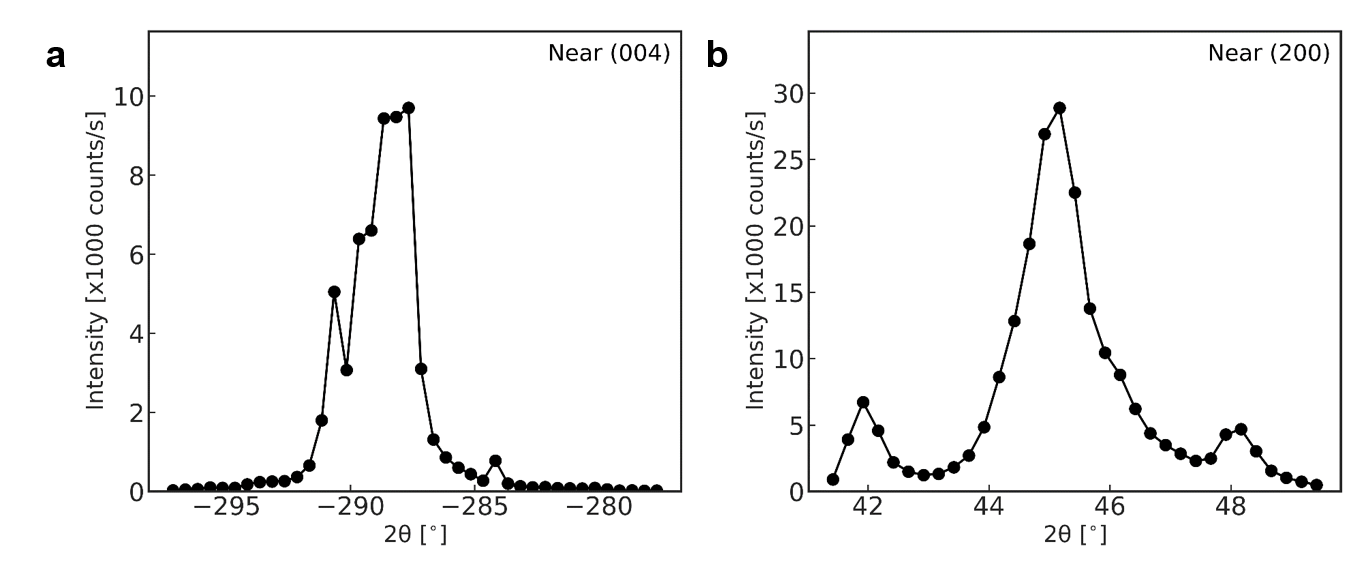
Figure S10: 2$\theta$-scans obtained from neutron diffraction scans of single-crystal TaP near Bragg peaks a, (004) and b, (200) at room temperature. Error bars representing one standard deviation are too small to be discernible.

X-ray and neutron diffraction. X-ray and neutron diffraction measurements of single-crystalline TaP were performed prior to performing the inelastic scattering measurements. These were required for the calculation of the orientation matrix used for alignment purposes and for the determination of the crystal lattice parameters at different temperatures. A couple of these scans near the elastic Bragg peaks at (004) and (200) obtained from neutron scattering are shown in Figure S10. Values obtained from both x-ray and neutron diffraction measurements at room temperature agree well with those obtained in Ref. xu_2015 ($a=b=3.32$Å and $c=11.34$Å).

Supplementary D: Computational details

All ab initio calculations are performed using the VASP kresse_1999; kresse_1996; kresse_1995 with projector-augmented-wave (PAW) pseudopotentials and Perdew-Burke-Ernzerhof (PBE) for exchange-correlation energy functional perdew_1996. The geometry optimization of the conventional cell was performed with a 6x6x2 Monkhorst-Pack grid of k-point sampling. The second-order and third-order force constants were calculated using a real space supercell approach with a 3x3x1 supercell. The Phonopy package was used to obtain the second-order force constants used in the calculation togo_2015.

Supplementary E: Phonon nesting conditions between Weyl nodes in TaP

In Table S1, we list the possible phonon nesting conditions for a phonon $\mathbf{q}=\mathbf{k}_{Wj_{1}}-\mathbf{k}_{Wj_{2}}$ between two Weyl electronic states at $\mathbf{k}_{Wj_{1}}$ and $\mathbf{k}_{Wj_{2}}$. Furthermore, we present the momentum-mismatch between phonon $\mathbf{q}$ and the Weyl node location in momentum-space $\mathbf{k}_{Wj^{\prime}}$ (which is reduced by the dynamical effect described in the main text) as well as the chirality of the two Weyl electronic states to highlight their conservation within the context of the topological Kohn anomaly in this material. The momentum-space coordinates of the 8 W1 ($k_{z}=0$) and 16 W2 ($k_{z}\neq 0$) Weyl nodes of TaP along with their respective chiralities are known from weng_2015.

Table S1: Possible phonon nesting conditions between different Weyl electronic states within TaP. Along with the momentum-space coordinates of the Weyl node in the Brillouin zone, the type and chirality of the electronic state is shown. Momentum conservation (presented in the form of a mismatch between nesting phonon $\mathbf{q}=\mathbf{k}_{1}-\mathbf{k}_{2}$ and the Weyl node location $\mathbf{k}_{Wj^{\prime}}$, i.e. |$\mathbf{q}-\mathbf{k}_{Wj}|/|\mathbf{k}_{Wj}|$ or $|\mathbf{q}|$ in the case of $\Gamma$) and the chirality conservation are featured in the table. Only one representative set for each case between Weyl nodes is shown with the number of instances indicated.

						Phonon	Momentum	Chirality
$\mathbf{k}_{1}$	Type	Chirality	$\mathbf{k}_{2}$	Type	Chirality	$\mathbf{q}$	conservation	conservation	Multiplicity
($+$0.271, $-$0.024, $+$0.578)	W2	+	($+$0.518, $+$0.014, $+$0.000)	W1	+	W2	4.35%	✓	16
($+$0.271, $+$0.024, $+$0.578)	W2	-	($+$0.518, $+$0.014, $+$0.000)	W1	+	W2	4.35%	$\times$	16
($-$0.271, $+$0.024, $+$0.578)	W2	+	($+$0.518, $+$0.014, $+$0.000)	W1	+	W2	4.49%	✓	16
($-$0.271, $-$0.024, $+$0.578)	W2	-	($+$0.518, $+$0.014, $+$0.000)	W1	+	W2	4.49%	$\times$	16
($+$0.024, $+$0.271, $+$0.578)	W2	+	($+$0.518, $+$0.014, $+$0.000)	W1	+	W2	34.98%	✓	16
($+$0.024, $-$0.271, $+$0.578)	W2	-	($+$0.518, $+$0.014, $+$0.000)	W1	+	W2	34.98%	$\times$	16
($-$0.024, $-$0.271, $-$0.578)	W2	+	($+$0.518, $+$0.014, $+$0.000)	W1	+	W2	42.48%	✓	16
($-$0.024, $+$0.271, $+$0.578)	W2	-	($+$0.518, $+$0.014, $+$0.000)	W1	+	W2	42.48%	$\times$	16
($+$0.271, $+$0.024, $+$0.578)	W2	-	($-$0.271, $+$0.024, $+$0.578)	W2	+	W1	5.36%	$\times$	16
($+$0.271, $+$0.024, $+$0.578)	W2	-	($+$0.271, $-$0.024, $+$0.578)	W2	+	W1	7.10%	$\times$	16
($+$0.271, $+$0.024, $+$0.578)	W2	-	($-$0.271, $-$0.024, $+$0.578)	W2	-	W1	8.03%	✓	16
($+$0.271, $+$0.024, $+$0.578)	W2	-	($+$0.271, $+$0.024, $-$0.578)	W2	-	W1	30.35%	✓	16
($+$0.271, $+$0.024, $+$0.578)	W2	-	($-$0.271, $+$0.024, $-$0.578)	W2	+	W1	30.58%	$\times$	16
($+$0.271, $+$0.024, $+$0.578)	W2	-	($+$0.271, $-$0.024, $-$0.578)	W2	+	W1	30.93%	$\times$	16
($+$0.271, $+$0.024, $+$0.578)	W2	-	($-$0.271, $-$0.024, $-$0.578)	W2	-	W1	31.16%	✓	16
($+$0.271, $+$0.024, $+$0.578)	W2	-	($-$0.024, $-$0.271, $+$0.578)	W2	+	W1	60.86%	$\times$	16
($+$0.271, $+$0.024, $+$0.578)	W2	-	($-$0.024, $+$0.271, $+$0.578)	W2	-	W1	62.24%	✓	16
($+$0.271, $+$0.024, $+$0.578)	W2	-	($+$0.024, $-$0.271, $+$0.578)	W2	-	W1	62.24%	✓	16
($+$0.271, $+$0.024, $+$0.578)	W2	-	($+$0.024, $+$0.271, $+$0.578)	W2	+	W1	63.59%	$\times$	16
($+$0.271, $+$0.024, $+$0.578)	W2	-	($-$0.024, $-$0.271, $-$0.578)	W2	+	W1	67.90%	$\times$	16
($+$0.271, $+$0.024, $+$0.578)	W2	-	($-$0.024, $+$0.271, $-$0.578)	W2	-	W1	69.14%	✓	16
($+$0.271, $+$0.024, $+$0.578)	W2	-	($+$0.024, $-$0.271, $-$0.578)	W2	-	W1	69.14%	✓	16
($+$0.271, $+$0.024, $+$0.578)	W2	-	($+$0.024, $+$0.271, $-$0.578)	W2	+	W1	70.36%	$\times$	16
($+$0.518, $+$0.014, $+$0.000)	W1	+	($+$0.518, $-$0.014, $+$0.000)	W1	-	$\Gamma$	2.80%	$\times$	8
($+$0.518, $+$0.014, $+$0.000)	W1	+	($-$0.518, $+$0.014, $+$0.000)	W1	-	$\Gamma$	49.30%	$\times$	8
($+$0.518, $+$0.014, $+$0.000)	W1	+	($-$0.518, $-$0.014, $+$0.000)	W1	+	$\Gamma$	49.38%	✓	8
($+$0.518, $+$0.014, $+$0.000)	W1	+	($+$0.014, $+$0.518, $+$0.000)	W1	-	$\Gamma$	71.28%	$\times$	8
($+$0.518, $+$0.014, $+$0.000)	W1	+	($-$0.014, $+$0.518, $+$0.000)	W1	+	$\Gamma$	73.28%	✓	8
($+$0.518, $+$0.014, $+$0.000)	W1	+	($+$0.014, $-$0.518, $+$0.000)	W1	+	$\Gamma$	73.28%	✓	8
($+$0.518, $+$0.014, $+$0.000)	W1	+	($-$0.014, $-$0.518, $+$0.000)	W1	-	$\Gamma$	75.24%	$\times$	8

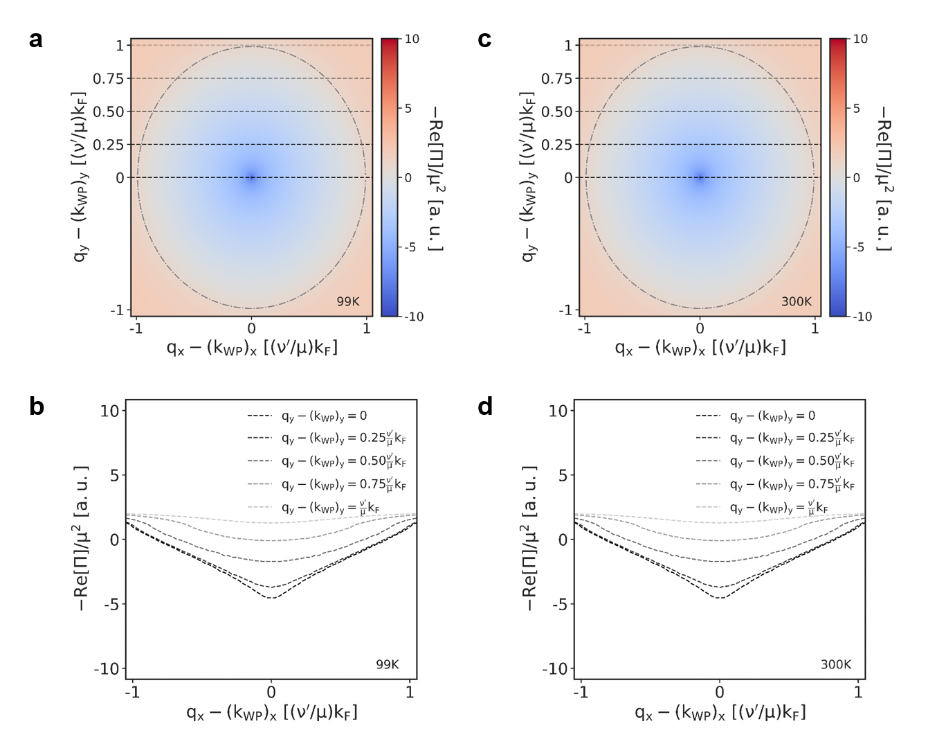
Figure S2: a. Density plot of $-\textrm{Re}[\Pi(\bm{q_{x}}-\bm{k_{\text{WP}_{x}}},\bm{q_{y}}-\bm{k_{\text{WP}_{y}}})]$ integrated over $0\leq\nu\leq\nu^{\prime}$ where the divergence is suppressed by additional terms in the denominator representative of other general scattering mechanics. Line cuts at different values of $\bm{q_{y}}-\bm{k_{\text{WP}_{y}}}=n(\nu^{\prime}/\mu)k_{F}$ where $n=0$, $0.25$, $0.5$, $0.75$ and $1$ are shown in b. c-d. Analogous to subfigures a-b, calculated at a temperature of 300K. The temperature dependence can be seen to be negligible from 1K up to 300K.

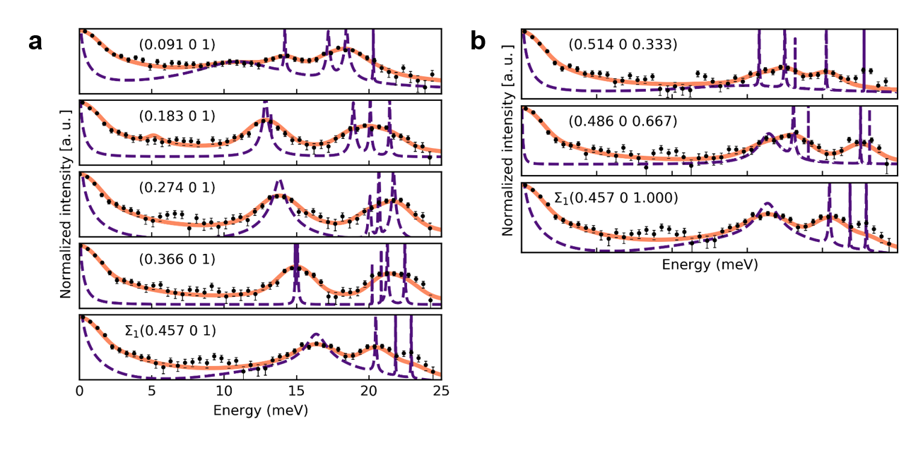
Figure S5: IXS data with statistical error taken at room temperature along high-symmetry line a, $Z-\Sigma_{1}$ and along b, $\Sigma-\Sigma_{1}$. The solid orange line denotes a least-squares fit to the intensity spectra from a damped harmonic oscillator function convoluted with the instrumental resolution function. The dashed purple line represents the resolution-deconvoluted phonon modes that contribute to the dispersion relation.

Figure S7: Representative intensity spectra obtained from inelastic neutron scattering (INS) performed with an energy range of 5-25 meV a, at the $\Gamma$ point, b, at a point along high symmetry direction $\Gamma$-$\Sigma$, $(0.217,0,0)$ and c, at a point along high symmetry direction $\Gamma$-Z, $(0,0,0.667)$. These spectra are in good agreement of phonon measurements performed with inelastic x-ray scattering. The solid lines are a guide for the eye.

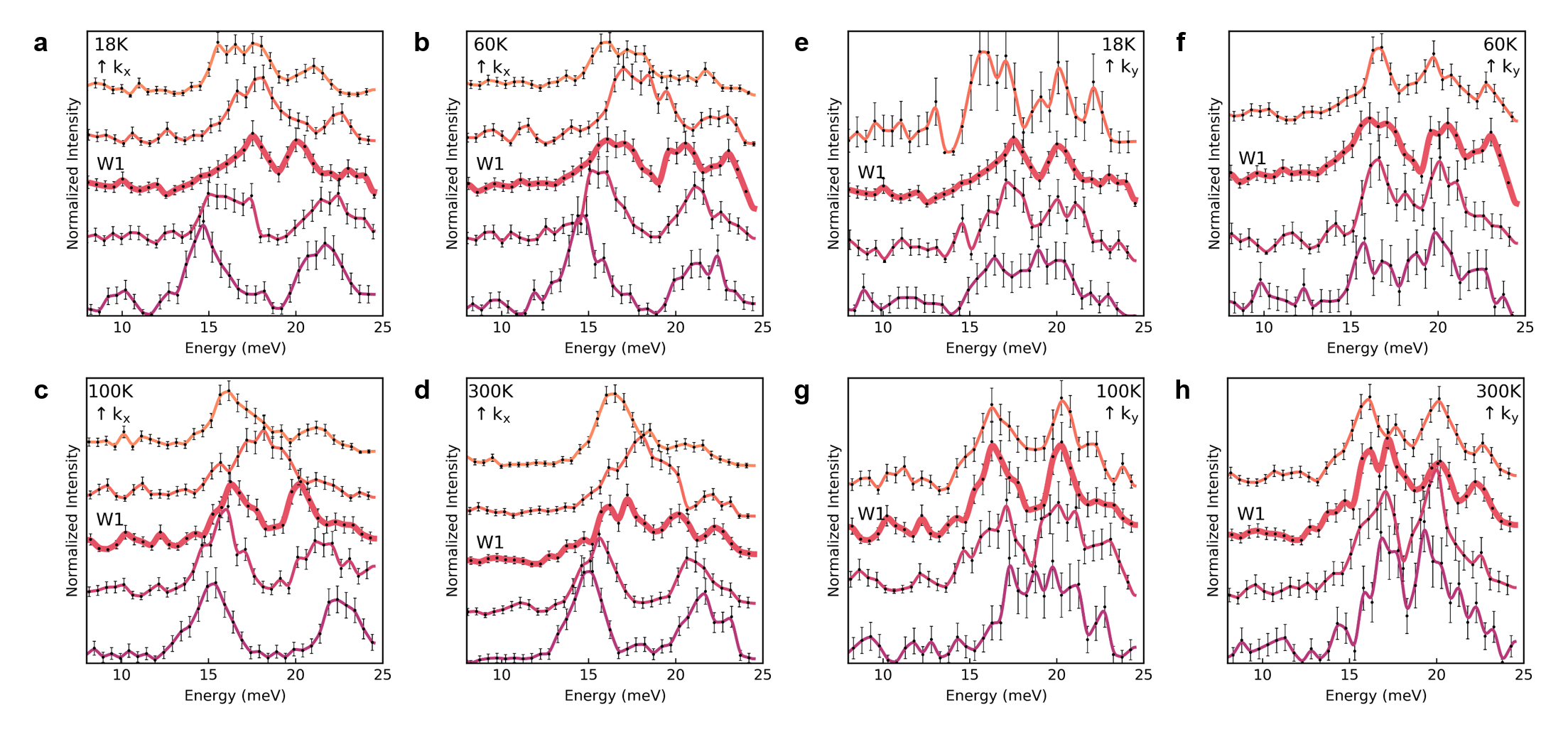
Figure S9: Momentum dependence of the intensity spectra with error bars near the W1 Weyl node at $(0.518,0.014,0)$. a-d display the IXS intensity spectra for $\bm{q}$-values along $H$ in $(H,0.014,0)$ for increasing $k_{x}$ direction from bottom to top at 18K, 60K, 100K and 300K, respectively. e-h display similar measurements at the same temperatures for $\bm{q}$-values along $K$ in $(0.518,K,0)$ for increasing $k_{y}$ direction from bottom to top. There are only four measurements due to instrumental limitations for larger $\bm{q}$-values. Lines serve as a guide to the eye. The central thicker line in each of the subfigures represents the IXS measurement performed directly at the W1 node.

References

[1]Note: See Supplementary Material at [url] for the complete derivation of the polarization and dielectric functions, which includes Refs. kapusta_2006; bjorken_1966; lv_2013; zhou_2015; thakur_2018; sadhukhan_2020.Cited by: Topological Singularity Induced Chiral Kohn Anomaly in a Weyl Semimetal.
[2]Note: See Supplementary Material at [url] for details on the single crystal growth, the x-ray and neutron scattering experiments and the data analysis, which includes Refs. han_2019; sinn_2001; alatas_2011; toellner_2011; lynn_2012; dave_2009.Cited by: Topological Singularity Induced Chiral Kohn Anomaly in a Weyl Semimetal.
A. Alatas, B. M. Leu, J. Zhao, H. Yavas, T. S. Toellner, and E. E. Alp (2011)Improved focusing capability for inelastic X-ray spectrometer at 3-ID of the APS: A combination of toroidal and Kirkpatrick-Baez (KB) mirrors.
Nuclear Instruments and Methods in Physics Research Section A: Accelerators, Spectrometers, Detectors and Associated Equipment649 (1), pp. 166–168 (en).
External Links: ISSN 0168-9002,
Link,
DocumentCited by: b_note2.
R. T. Azuah, L. R. Kneller, Y. Qiu, P. L. W. Tregenna-Piggott, C. M. Brown, J. R. D. Copley, and R. M. Dimeo (2009)DAVE: A Comprehensive Software Suite for the Reduction, Visualization, and Analysis of Low Energy Neutron Spectroscopic Data.
Journal of Research of the National Institute of Standards and Technology114 (6), pp. 341–358 (eng).
External Links: ISSN 1044-677X,
DocumentCited by: b_note2.
J. D. Bjorken, S. D. Drell, and P. B. Kahn (1966)Relativistic Quantum Fields.
American Journal of Physics34 (4), pp. 367–367 (en).
External Links: ISSN 0002-9505, 1943-2909,
Link,
DocumentCited by: a_note1.
K. C. Fu, C. Santori, P. E. Barclay, L. J. Rogers, N. B. Manson, and R. G. Beausoleil (2009)Observation of the dynamic jahn-teller effect in the excited states of nitrogen-vacancy centers in diamond.
Phys. Rev. Lett.103, pp. 256404.
External Links: Document,
LinkCited by: Topological Singularity Induced Chiral Kohn Anomaly in a Weyl Semimetal.
F. Han, N. Andrejevic, T. Nguyen, V. Kozii, Q. Nguyen, Z. Ding, R. Pablo-Pedro, S. Parjan, B. Skinner, A. Alatas, E. Alp, S. Chi, J. Fernandez-Baca, S. Huang, L. Fu, and M. Li (2019)Discovery of Giant, Non-saturating Thermopower in Topological Semimetal at Quantum Limit.
arXiv:1904.03179 [cond-mat].
External Links: LinkCited by: b_note2.
S. Huang, S. Xu, I. Belopolski, C. Lee, G. Chang, B. Wang, N. Alidoust, G. Bian, M. Neupane, C. Zhang, S. Jia, A. Bansil, H. Lin, and M. Z. Hasan (2015)A Weyl Fermion semimetal with surface Fermi arcs in the transition metal monopnictide TaAs class.
Nature Communications6 (1), pp. 1–6 (en).
External Links: ISSN 2041-1723,
Link,
DocumentCited by: Topological Singularity Induced Chiral Kohn Anomaly in a Weyl Semimetal.
J. I. Kapusta and C. Gale (2006)Finite-temperature field theory: principles and applications.
2nd ed edition, Cambridge University Press.
Cited by: a_note1.
D. Kozawa, R. Kumar, A. Carvalho, K. Kumar Amara, W. Zhao, S. Wang, M. Toh, R. M. Ribeiro, A. H. Castro Neto, K. Matsuda, and G. Eda (2014)Photocarrier relaxation pathway in two-dimensional semiconducting transition metal dichalcogenides.
Nature Communications5 (1), pp. 1–7 (en).
External Links: ISSN 2041-1723,
Link,
DocumentCited by: Topological Singularity Induced Chiral Kohn Anomaly in a Weyl Semimetal.
G. Kresse, J. Furthmüller, and J. Hafner (1995)Ab initio Force Constant Approach to Phonon Dispersion Relations of Diamond and Graphite.
Europhysics Letters (EPL)32 (9), pp. 729–734.
External Links: ISSN 0295-5075, 1286-4854,
Link,
DocumentCited by: c_note3.
G. Kresse and J. Furthmüller (1996)Efficiency of ab-initio total energy calculations for metals and semiconductors using a plane-wave basis set.
Computational Materials Science6 (1), pp. 15–50 (en).
External Links: ISSN 0927-0256,
Link,
DocumentCited by: c_note3.
G. Kresse and D. Joubert (1999)From ultrasoft pseudopotentials to the projector augmented-wave method.
Phys. Rev. B59, pp. 1758–1775.
External Links: Document,
LinkCited by: c_note3.
B. Q. Lv, N. Xu, H. M. Weng, J. Z. Ma, P. Richard, X. C. Huang, L. X. Zhao, G. F. Chen, C. E. Matt, F. Bisti, V. N. Strocov, J. Mesot, Z. Fang, X. Dai, T. Qian, M. Shi, and H. Ding (2015)Observation of Weyl nodes in TaAs.
Nature Physics11 (9), pp. 724–727 (en).
External Links: ISSN 1745-2481,
Link,
DocumentCited by: Topological Singularity Induced Chiral Kohn Anomaly in a Weyl Semimetal.
M. Lv and S. Zhang (2013)Dielectric function, friedel oscillation and plasmons in weyl semimetals.
International Journal of Modern Physics B27 (25), pp. 1350177.
External Links: ISSN 0217-9792,
Link,
DocumentCited by: a_note1.
J. W. Lynn, Y. Chen, S. Chang, Y. Zhao, S. Chi, W. Ratcliff, B. G. Ueland, and R. W. Erwin (2012)Double-Focusing Thermal Triple-Axis Spectrometer at the NCNR.
Journal of Research of the National Institute of Standards and Technology117, pp. 61–79.
External Links: ISSN 1044-677X,
Link,
DocumentCited by: b_note2.
C. Min, H. Bentmann, J. N. Neu, P. Eck, S. Moser, T. Figgemeier, M. Ünzelmann, K. Kissner, P. Lutz, R. J. Koch, C. Jozwiak, A. Bostwick, E. Rotenberg, R. Thomale, G. Sangiovanni, T. Siegrist, D. Di Sante, and F. Reinert (2019)Orbital fingerprint of topological fermi arcs in the weyl semimetal tap.
Phys. Rev. Lett.122, pp. 116402.
External Links: Document,
LinkCited by: Topological Singularity Induced Chiral Kohn Anomaly in a Weyl Semimetal.
J. P. Perdew, K. Burke, and M. Ernzerhof (1996)Generalized gradient approximation made simple.
Phys. Rev. Lett.77, pp. 3865–3868.
External Links: Document,
LinkCited by: c_note3.
D. Reznik, L. Pintschovius, M. Ito, S. Iikubo, M. Sato, H. Goka, M. Fujita, K. Yamada, G. D. Gu, and J. M. Tranquada (2006)Electron-phonon coupling reflecting dynamic charge inhomogeneity in copper oxide superconductors.
Nature440, pp. 1170–1173.
External Links: LinkCited by: Topological Singularity Induced Chiral Kohn Anomaly in a Weyl Semimetal.
K. Sadhukhan, A. Politano, and A. Agarwal (2020)Novel Undamped Gapless Plasmon Mode in a Tilted Type-II Dirac Semimetal.
Physical Review Letters124 (4), pp. 046803.
External Links: Link,
DocumentCited by: a_note1.
H. Sinn, E. E. Alp, A. Alatas, J. Barraza, G. Bortel, E. Burkel, D. Shu, W. Sturhahn, J. P. Sutter, T. S. Toellner, and J. Zhao (2001)An inelastic X-ray spectrometer with 2.2meV energy resolution.
Nuclear Instruments and Methods in Physics Research Section A: Accelerators, Spectrometers, Detectors and Associated Equipment467-468, pp. 1545–1548 (en).
External Links: ISSN 0168-9002,
Link,
DocumentCited by: b_note2.
A. Thakur, K. Sadhukhan, and A. Agarwal (2018)Dynamic current-current susceptibility in three-dimensional Dirac and Weyl semimetals.
Physical Review B97 (3), pp. 035403.
External Links: Link,
DocumentCited by: a_note1.
T. S. Toellner, A. Alatas, and A. H. Said (2011)Six-reflection meV-monochromator for synchrotron radiation.
Journal of Synchrotron Radiation18 (4), pp. 605–611.
External Links: ISSN 0909-0495,
Link,
DocumentCited by: b_note2.
A. Togo and I. Tanaka (2015)First principles phonon calculations in materials science.
Scripta Materialia108, pp. 1–5 (en).
External Links: ISSN 1359-6462,
Link,
DocumentCited by: c_note3.
S. Xu, I. Belopolski, N. Alidoust, M. Neupane, G. Bian, C. Zhang, R. Sankar, G. Chang, Z. Yuan, C. Lee, S. Huang, H. Zheng, J. Ma, D. S. Sanchez, B. Wang, A. Bansil, F. Chou, P. P. Shibayev, H. Lin, S. Jia, and M. Z. Hasan (2015)Discovery of a weyl fermion semimetal and topological fermi arcs.
Science349 (6248), pp. 613–617.
External Links: Document,
ISSN 0036-8075,
LinkCited by: Topological Singularity Induced Chiral Kohn Anomaly in a Weyl Semimetal.
S. Yue, H. T. Chorsi, M. Goyal, T. Schumann, R. Yang, T. Xu, B. Deng, S. Stemmer, J. A. Schuller, and B. Liao (2019)Soft phonons and ultralow lattice thermal conductivity in the Dirac semimetal ${\mathrm{Cd}}_{3}{\mathrm{As}}_{2}$.
Physical Review Research1 (3), pp. 033101.
External Links: Link,
DocumentCited by: Topological Singularity Induced Chiral Kohn Anomaly in a Weyl Semimetal.
J. Zhou, H. Chang, and D. Xiao (2015)Plasmon mode as a detection of the chiral anomaly in Weyl semimetals.
Physical Review B91 (3), pp. 035114.
External Links: Link,
DocumentCited by: a_note1.
X. Zhu, L. Santos, C. Howard, R. Sankar, F. C. Chou, C. Chamon, and M. El-Batanouny (2012)Electron-phonon coupling on the surface of the topological insulator determined from surface-phonon dispersion measurements.
Phys. Rev. Lett.108, pp. 185501.
External Links: Document,
LinkCited by: Topological Singularity Induced Chiral Kohn Anomaly in a Weyl Semimetal.