Reduced density matrix of nonlocal identical particles

Abstract

We probe the theoretical connection among three different approaches to analyze the entanglement of identical particles, i.e., the first quantization language (1QL), elementary-symmetric/exterior products (which has the mathematical equivalence to no-labeling approaches), and the algebraic approach based on the GNS construction. Among several methods to quantify the entanglement of identical particles, we focus on the computation of reduced density matrices, which can be achieved by the concept of symmetrized partial trace defined in 1QL. We show that the symmetrized partial trace corresponds to the interior product in symmetric and exterior algebra (SEA), which also corresponds to the subalgebra restriction in the algebraic approach based on GNS representation. Our research bridges different viewpoints for understanding the quantum correlation of identical particles in a consistent manner.

1 Introduction

Quantum entanglement is one of the crucial quantum concepts which reveals the essential feature of quantum physics. It implies the possibility of composite systems that cannot be described as a simple collection of individual subsystems, even when the subsystems locate far from each other [1, 2]. It is also exploited as a crucial resource to enable several tasks with quantum speedup [3]. One of the insightful approaches to analyze the entanglement of a given quantum system is to use the partial trace technic. Intuitively, if a multipartite quantum system is entangled, a subsystem of the quantum system has some nonlocal (measurement-dependent) correlation with the “outer world” in the total system. The information on the correlation is encoded in the reduced density matrix, a quantum state acquired by partial tracing the outer part of the total state.

For the case of non-identical particles, in which each particle resides in a distinguished Hilbert space, the concept of the partial trace is well-defined. On the other hand, in the case of identical particles (both bosons and fermions), individual particles do not reside in independent Hilbert spaces, by which the concept of partial trace seems inappropriate to obtain reduced density matrices suitable for analyzing the entanglement of identical particles. Several alternatives have been suggested to overcome this problem.

An algebraic approach (AA) based on Gel’fand-Naimark-Segel (GNS) construction is suggested by Balachandran et al. [4, 5]. They demonstrated that, instead of partial trace, a restriction to a chosen subalgebra of observables provides a sound tool to compute the entanglement entropy (the importance of subalgebras for interpreting the entanglement of identical particles in the second quantization language (2QL) is also pointed out in Ref. [6, 7, 8]). On the other hand, a no-labelling approach (NLA) [9, 10, 11] describes the identical particles without introducing particle pseudo-labels. By extracting the transition relations of wave functions from the symmetric properties of identical particles, partial trace can be defined in the no-labeling formalism (the same process was reproduced in the second quantization language in Ref. [12]). Also, the concept of symmetrized partial trace for identical particles in the first quantization language (1QL) was introduced in Ref. [13]. By applying the symmetrization principle for identical particles not only to wavefunctions but also to detectors, the reduced density matrix that preserves the particle label symmetry can be derived (for more discussions on the entanglement of identical particles from various viewpoints, see Refs. [14, 15, 16, 17, 18, 19, 20, 21, 22, 23, 24, 25, 26, 27, 28, 29]).

Hence, one can state that there exists a seemingly incompatible standpoint on the validity of the partial trace in the problem of entanglement of identical particles. However, considering that all the above theories deal with the same physical systems, one can surmise that this seeming inconsistency must be reconciled by examining the resultant quantities or the formal structures. In this work, we show how the aforementioned different approaches can translate and provide fundamentally equivalent results to each other.

In the course of delving into the issue, we utilize the elementary symmetric product (for bosons) and the exterior product (for fermions) to demonstrate the indistinguishability and projection rules for identical particles. It will be shown that the symmetrized partial trace of identical particles is equivalent to the interior products between elementary symmetric (for bosons) and exterior (for fermions) state vectors, which is equivalent to the restriction to a subalgebra on GNS representation.

Section 2 explains the first quantization language (1QL) and the concept of symmetrized partial trace. Section 3 shows how 1QL can be translated to the symmetric and exterior algebra (SEA). Then Section 4 shows that reduced density matrix computed in SEA is the same matrix computed using the concept of restriction to subalgebras in the algebraic approach introduced in Refs. [4, 5].

2 The first quantization language

To describe the identical particles in 1QL, we start with the description of $N$ non-identical particles. For this case, since we can “distinguish” the particles fully, each particle has inherent physical labels that are different from each other. A particle with label A in a state $\Psi$ is described by $|\Psi\rangle_{A}$, where $\Psi$ includes the position $\psi$ and internal state $s$, i.e., $\Psi=(\psi,s)$. The total $N$-particle state is given by

$$|\Psi_{1}\rangle_{1}\otimes|\Psi_{2}\rangle_{2}\otimes\cdots\otimes|\Psi_{N}\rangle_{N},$$ (1)

where the subscripts outside the kets denote the particle labels. Since the transition amplitude of $|\Psi\rangle_{A}$ to another state $|\Phi\rangle_{B}$ is given by

$$_{A}\langle\Phi|\Psi\rangle_{B}=\langle\Phi|\Psi\rangle\delta_{AB},$$ (2)

the transition amplitude from a $N$-particle state $|\Psi_{1}\rangle_{1}\otimes|\Psi_{2}\rangle_{2}\otimes\cdots\otimes|\Psi_{N}\rangle_{N}$ to $|\Phi_{1}\rangle_{1}\otimes|\Phi_{2}\rangle_{2}\otimes\cdots\otimes|\Phi_{N}\rangle_{N}$ is computed as

$$\langle\Phi_{1}|\Psi_{1}\rangle\langle\Phi_{2}|\Psi_{2}\rangle\cdots\langle\Phi_{N}|\Psi_{N}\rangle.$$ (3)

Or, one can omit the labels, by supposing that the order of particle states represents the labels. Then Eq. (1) is rewritten as

$$|\Psi_{1}\rangle\otimes|\Psi_{2}\rangle\otimes\cdots\otimes|\Psi_{N}\rangle$$ (4)

and the transition amplitude is given in the same form as Eq. (3). We call the expressions Eq. (1) and Eq. (4) explicit/implicit notation respectively. However, one should be aware that a ket $|\Psi_{i}\rangle$ in the implicit notation is different from the same ket in Eq. (3). The kets in Eq. (4) implicitly contain the information on particle labels by their relative order, which is absent in the kets in Eq. (3). Hence, we use the explicit notation to avoid the confusion in this text. Appendix A explains the implicit description of identical particles and compares it with the explicit description that we will discuss from now on.

Since identical particles have the exchange symmetry, the total state of $N$ identical particles in states $\Psi_{i}$ ($i=1,\dots,N$) with particle labels $A_{a}$ ($a=1,\dots,N$ and $A_{a}\neq A_{b}$ for $a\neq b$) is expressed as

$$|\Psi\rangle^{\pm}\equiv|\Psi_{1},\Psi_{2},\cdots,\Psi_{N}\rangle^{\pm}={\mathcal{N}}(\Psi)\Big{[}\sum_{\sigma\in S_{N}}(\pm 1)^{\sigma}|\Psi_{1}\rangle_{A_{\sigma(1)}}|\Psi_{2}\rangle_{A_{\sigma(2)}}\cdots|\Psi_{N}\rangle_{A_{\sigma(N)}}\Big{]},$$ (5)

where the sign $+$ is for bosons and $-$ for fermions. ${\mathcal{N}}(\Psi)$ is the normalization factor of $|\Psi_{1},\Psi_{2},\cdots,\Psi_{N}\rangle$. Since identical particles cannot be addressed individually, the particle labels are not physical, i.e., “pseudo-labels” [13]. With Eq. (2), the transition amplitude from $|\Psi_{1},\cdots,\Psi_{N}\rangle^{\pm}$ to $|\Phi_{1},\cdots,\Phi_{N}\rangle^{\pm}$ is computed as

$$\langle\Phi_{1},\cdots,\Phi_{N}|\Psi_{1},\cdots,\Psi_{N}\rangle^{\pm}={\mathcal{N}}(\Phi){\mathcal{N}}(\Psi)\sum_{\rho,\sigma}(\pm 1)^{\rho}(\pm 1)^{\sigma}\prod_{i=1}^{N}\langle\Phi_{\rho(i)}|\Psi_{\sigma(i)}\rangle.$$ (6)

By the definition of a matrix $A$ with imposed as $A_{ij}=\langle\Phi_{i}|\Psi_{j}\rangle$, Eq. (6) is proportional to the matrix permanent and determinant of $A$ for bosons and fermions repectively.

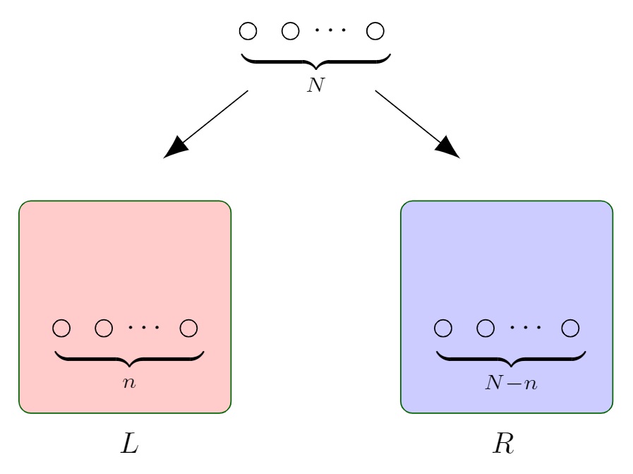
Figure 1: $N$ identical particles distributed in two distinctive subsystems $L$ and $R$. The two sets of identical particles ($n,N-n$) can have nontrivial correlation with nonzero spatial coherence [10, 13].

Our bipartite entanglement of identical particles presupposes the division of the particles into two distinguished spatial modes (Fig. 1). The expression of $n$ ($\leq N$) identical particle partial wavefunctions in 1QL needs extra attention, for in this case we have no information on which of the $N$ particles are in which mode. The partial wavefunction $|\Psi_{1},\cdots,\Psi_{n}\rangle$ for the subsystem should be symmetrized with respect to the $N$ particle pseudolabels. The most general form that satisfies the exchange symmetry is given by

$$|\Psi_{1},\cdots,\Psi_{n}\rangle^{\pm} =\mathcal{N}_{[n]}(\Psi)\sum_{\begin{subarray}{c}a_{1}<\cdots<a_{n}\\ =1\end{subarray}}^{N}e^{i\theta_{a_{1}\cdots a_{n}}}\sum_{\sigma\in S_{n}}(\pm 1)^{\sigma}|\Psi_{1}\rangle_{A_{a_{1}}}\cdots|\Psi_{n}\rangle_{A_{a_{n}}},$$ (7)

where $1\leq a_{p}\leq N$ for all $p=1,\cdots,n$ and ${\mathcal{N}}_{[n]}$ is the normalization factor. Note that $\theta_{a_{1}\cdots a_{n}}$ for each $\{a_{1},\cdots,a_{n}\}$ does not affect the anti-symmetric property of the subsystem state, hence can be chosen arbitrarily . All the phases $\theta_{a_{1}\cdots a_{n}}$ can be set to zero for the case of bosons [13], which is however not true for fermions (see Appendix B for a more detailed explanation).

With Eq. (7), we can define the partial trace of a given density marix $\rho$ over a subsystem S with $n$ identical particles. Since the resultant reduced density matrix also preserves the pseudolabel exchange symmetry, the partial trace for identical particles in 1QL is dubbed symmetrized partial trace [13]. Supposing $\{|\Phi_{1}^{a},\cdots,\Phi_{n}^{a}\rangle\}_{a}$ composes the complete symmetric computational basis set of $n$ particles in the subsystem $S$, the identity matrix for $S$ is expressed with

$$\mathbb{I}_{S}=\sum_{n\in SSR}\sum_{a}|\Phi_{1}^{a},\cdots,\Phi_{n}^{a}\rangle\langle\Phi_{1}^{a},\cdots,\Phi_{n}^{a}|$$ (8)

where the summation over $n$ means that we have to add the states for all possible $n$ that preserve the superselection rules (SSR, the particle number and parity SSR for bosons and fermions respectively [30, 31, 32]). Then the reduced density matrix of the subsystem $\bar{S}$ by the symmetrized partial trace over $S$ is given by

$$\rho_{\bar{S}}={\rm Tr}_{S}(\rho)\equiv\sum_{n\in SSR}\sum_{a}\langle\Phi_{1}^{a},\dots,\Phi_{n}^{a}|\rho|\Phi_{1}^{a},\dots,\Phi_{n}^{a}\rangle.$$ (9)

With the reduced density matrix $\rho_{\bar{S}}$, we can evaluate the amount of entanglement that is detectable and physical. Appendix B provides an $(N,n)=(3,1)$ fermionic example. One can see that the extension of the argument to a mixed state case $\rho=\sum_{a}\psi_{a}|\Psi_{a}\rangle\langle\Psi_{a}|$ ($\psi_{a}\in\mathbb{R}^{+}$, $\sum_{a}\psi_{a}=1$) is straightforward .

3 From 1QL to symmetric-exterior algebraic (SEA) approach

The computations in Sec. 2 can be reproduced using the tensor algebra methods with suitable symmetries for identical particles. In this section, we provide a mathematical analysis on the relation of 1QL with the symmetric-exterior algebra (SEA). We show that a bosonic wavefunction in 1QL corresponds to an elementary symmetric vector in the symmetric algebra, which can be straightforwardly extended to the relation between fermionic wavefunctions in 1QL and exterior vectors.

From a given element $x$ of a tensor algebra, one can impose an exchange symmetry with a proper mapping. Let $\{{\hat{e}}_{1},\cdots,{\hat{e}}_{N}\}$ be a basis set of the $N$-dimensional vector space $V$ and $\{{\hat{e}}^{*1},\cdots,{\hat{e}}^{*N}\}$ its dual, so that the inner product among them is given by $({\hat{e}}_{a},{\hat{e}}^{*b})=\delta_{a}^{b}$. Then we define the elementary symmetrizing map $S^{(k)}_{e}(x)$ of the element $x$ as follows:

Definition 1.

For a $k$-th tensor power $T^{k}V$ of a vector space $V$ ($=\overbrace{V\otimes\cdots\otimes V}^{k}$) and a $k$-vector $x=\sum_{i_{1},\cdots,i_{k}}x^{i_{1}\cdots i_{k}}{\hat{e}}_{i_{1}}\otimes\cdots\otimes{\hat{e}}_{i_{k}}$ in $T^{k}V$, the elementary symmetrizing map $S^{(k)}_{e}(x)$ is defined as

$$S_{e}^{(k)}(x)=\sum_{i_{1},\cdots,i_{k}}x^{i_{1}\cdots i_{k}}S_{e}^{(k)}({\hat{e}}_{i_{1}}\otimes\cdots\otimes{\hat{e}}_{i_{k}})$$ (10)

where

$$S_{e}^{(k)}({\hat{e}}_{i_{1}}\otimes\cdots\otimes{\hat{e}}_{i_{k}})=\frac{1}{k!}\sum_{a_{1},\cdots,a_{k}=1}^{k}|\epsilon_{i_{a_{1}}\cdots i_{a_{k}}}|({\hat{e}}_{i_{a_{1}}}\otimes\cdots\otimes{\hat{e}}_{i_{a_{k}}})$$ (11)

($|\epsilon_{i_{a_{1}},\cdots,i_{a_{k}}}|$ is the absolute value of the Levi-Civita symbol, which vanishes when $i_{a_{k}}=i_{a_{l}}$ for any $k$ and $l$).

Note that the elementary symmetrizing map $S_{e}^{(k)}$ projects out any elements of $x$ that satisfy $i_{a}=i_{b}$ ($1\leq a,b\leq k$). For example, when $x=\sum_{i,j=1}^{N}x^{ij}({\hat{e}}_{i}\otimes{\hat{e}}_{j})$, we have

$$S_{e}^{(2)}(x) =\sum_{i,j}x^{ij}S_{e}^{(2)}({\hat{e}}_{i}\otimes{\hat{e}}_{j})=\frac{1}{2}\sum_{i,j}x^{ij}|\epsilon_{ij}|({\hat{e}}_{i}\otimes{\hat{e}}_{j}+{\hat{e}}_{j}\otimes{\hat{e}}_{i})$$

$$=\sum_{i\neq j}\Big{(}\frac{x^{ij}+x^{ji}}{2}\Big{)}\Big{(}\frac{{\hat{e}}_{i}\otimes{\hat{e}}_{j}+{\hat{e}}_{j}\otimes{\hat{e}}_{i}}{2}\Big{)}.$$ (12)

The elementary symmetrizing map is simply denoted with the the elementary symmetric product $\vee$ as

$$v\vee w\equiv S_{e}^{(k)}(v\otimes w)$$ (13)

where $v\in T^{l}V$ and $w\in T^{(k-l)}V$ ($0\leq l\leq k$).

Definition 1 gives a direct relation of a $N$ boson state in 1QL with the symmetric algebra. By defining $|{\hat{\Psi}}_{i}\rangle=\frac{1}{\sqrt{N}}\sum_{a=1}^{N}|\Psi_{i}\rangle_{A_{a}}{\hat{e}}^{*a}$, which is a vector in $V$ that is invariant under the exchange of pseudolabels, we can directly see that an $N$-boson total state $|\Psi\rangle^{+}$ (Eq. (5)) is related to an elementary symmetric $N$-vector as (note that the equalities hold upto normalization)

$$|\Psi\rangle^{+} =\sum_{\sigma\in S_{N}}|\Psi_{1}\rangle_{A_{\sigma(1)}}|\Psi_{2}\rangle_{A_{\sigma(2)}}\cdots|\Psi_{N}\rangle_{A_{\sigma(N)}}$$

$$=\sum_{\begin{subarray}{c}k_{1}<\cdots<k_{N}\\ =1\end{subarray}}^{N}({\hat{e}}_{k_{1}}\vee\cdots\vee{\hat{e}}_{k_{N}},|{\hat{\Psi}}_{1}\rangle\vee\cdots\vee|{\hat{\Psi}}_{N}\rangle)\equiv F^{+}(|{\hat{\Psi}}_{1}\rangle\vee\cdots\vee|{\hat{\Psi}}_{N}\rangle).$$ (14)

Here $(v,w)$ is the inner product between two $k$-vectors $v$ and $w$. And the $n$-boson subsystem state Eq. (7) is written as

$$|\Psi_{1},\cdots,\Psi_{n}\rangle^{+}$$

$$=\sum_{\begin{subarray}{c}a_{1}<\cdots<a_{n}\\ =1\end{subarray}}^{N}e^{i\theta_{a_{1}\cdots a_{n}}}\sum_{\sigma\in S_{n}}|\Psi_{1}\rangle_{A_{\sigma(a_{1})}}\cdots|\Psi_{n}\rangle_{A_{\sigma(a_{n})}}$$

$$=\sum_{k_{1}<\cdots<k_{n}=1}^{N}e^{i\theta_{k_{1}\cdots k_{n}}}({\hat{e}}_{A_{k_{1}}}\vee\cdots\vee{\hat{e}}_{A_{k_{n}}},|{\hat{\Psi}}_{1}\rangle\vee\cdots\vee|{\hat{\Psi}}_{n}\rangle).$$ (15)

Note that the phase ambiguity of Eq. (7) can be restricted to the complex coefficients of the $n$-dimensional basis vectors ${\hat{e}}_{A_{k_{1}}}\vee\cdots\vee{\hat{e}}_{A_{k_{n}}}$ in Eq. (3). Considering the phase ambiguity is a purely mathematical feature that has no physical implication, one can state that $|{\hat{\Psi}}_{1}\rangle\vee\cdots\vee|{\hat{\Psi}}_{n}\rangle$ ($1\leq n\leq N$) have the complete physical information on the total and sub- states for a set of identical bosons. Hence, any subset of a given $N$ identical bosons can be exactly represented as an elementary symmetric product of single particle vectors $|{\hat{\Psi}}_{i}\rangle$ that is invariant under pseudolable exchanges. From now on, we call such vectors “elementary symmetric state vectors.”

The connection of bosonic states to the exterior state vectors provides an intriguing insight on our physical system. Since an elementary symmetric state vector $|{\hat{\Psi}}_{i_{1}}\rangle\vee\cdots\vee|{\hat{\Psi}}_{i_{n}}\rangle$ ($1\leq i_{a}\leq N$, ${}^{\forall}a=1,\cdots,n$) is in the $n$th symmetric power $\bigvee^{n}(V)$ ($1\leq n\leq N$), all the possible subsets of identical fermions construct the complete set of the graded structure, i.e., $\{|{\hat{\Psi}}_{i_{1}}\rangle\vee\cdots\vee|{\hat{\Psi}}_{i_{n}}\rangle\}_{n=1}^{N}$ $\simeq$ $\oplus_{n=1}^{N}\bigvee^{n}(V)$. We can see that the projection between identical particle states corresponds to the shift in the graded structure. Considering the bra states $\langle\Psi_{n},\cdots,\Psi_{1}|$ ($\equiv(|\Psi_{1},\cdots,\Psi_{n}\rangle)^{\dagger}$) are expressed likewise with the symmetric products of $\langle{\hat{\Psi}}_{i}|=\sum_{a}\langle\Psi_{i}|^{A_{a}}e_{A_{a}}$, one can see that the projection of $|\Phi_{1},\cdots,\Phi_{m}\rangle$ onto $|\Psi_{1},\cdots,\Psi_{n}\rangle$ ($1\leq n\leq m\leq N$) is replaced with the interior products of $\langle{\hat{\Phi}}_{n}|\vee\cdots\vee\langle{\hat{\Phi}}_{1}|$ and $|{\hat{\Psi}}_{1}\rangle\vee\cdots\vee|{\hat{\Psi}}_{m}\rangle$. For example, when $n=1$, the interior product of $\langle{\hat{\Phi}}_{1}|$ and $|{\hat{\Psi}}_{1}\rangle\vee\cdots\vee|{\hat{\Psi}}_{m}\rangle$ is given by

$$\langle{\hat{\Phi}}_{1}|\cdot|{\hat{\Psi}}_{1}\rangle\vee\cdots\vee|{\hat{\Psi}}_{m}\rangle$$

$$=\sum_{j}\langle\Phi_{1}|\Psi_{j}\rangle|{\hat{\Psi}}_{1}\rangle\vee\cdots\vee(|{\hat{\Psi}}_{j}\rangle)\vee|{\hat{\Psi}}_{m}\rangle$$ (16)

(here $(|{\hat{\Psi}}_{j}\rangle)$ means that $|{\hat{\Psi}}_{j}\rangle$ is absent in the exterior state vector). For $n=2$, we have

$$\langle{\hat{\Phi}}_{1}|\vee\langle{\hat{\Phi}}_{2}|\cdot|{\hat{\Psi}}_{1}\rangle\vee\cdots\vee|{\hat{\Psi}}_{m}\rangle$$

$$=\langle{\hat{\Phi}}_{1}|\cdot(\langle{\hat{\Phi}}_{2}|\cdot|{\hat{\Psi}}_{1}\rangle\vee\cdots\vee|{\hat{\Psi}}_{m}\rangle)$$

$$=\sum_{j}(-1)^{j-1}\langle\Phi_{2}|\Psi_{j}\rangle(\langle{\hat{\Phi}}_{1}|\cdot|{\hat{\Psi}}_{1}\rangle\vee\cdots\vee(|{\hat{\Psi}}_{j}\rangle)\vee|{\hat{\Psi}}_{m}\rangle)$$

$$=\sum_{j,k}(-1)^{j+k}\langle\Phi_{1}|\Psi_{j}\rangle\langle\Phi_{2}|\Psi_{k}\rangle$$

$$\qquad\quad\times\Big{[}|{\hat{\Psi}}_{1}\rangle\vee\cdots\vee(|{\hat{\Psi}}_{j}\rangle)\vee\cdots\vee(|{\hat{\Psi}}_{j}\rangle)\vee\cdots\vee|{\hat{\Psi}}_{m}\rangle\Big{]}.$$ (17)

The same operation can be applied to an arbitrary $n$.

a set of identical particles	tensor algebra
bosonic state	elementary symmetric vector
(fermionic state)	(exterior vector)
symmetric partial trace	interior product
subsystems	graded structure

Table 1: The translation relation between 1QL and SEA for the description of identical particle entanglement

By replacing the state vectors of Eqs. (8) and (9) with the corresponding elementary symmetric state vectors, we can calculate the reduced density matrix in a given subsystem with Eqs. (3) and (3). The algebraic relation of states defined in NLA [11] is equal to the interior product Eq. (3), which means that the physical states in NLA are operationally equivalent to the elementary symmetric vectors.

We can analyze the entanglement of fermions in the same way by replacing the elementary symmetric algebra with the exterior (antisymmetric) algebra [33]. The relation of the physical systems of identical particles with tensor algebras is summarized in Table 1. Appendix A presents another way of describing identical particles using SEA with the implicit notation.

We can state that the tensor product $\otimes$ for the entanglement of non-identical particles is replaced with the elementary symmetric product $\vee$ and the exterior product $\wedge$ for bosons and fermions respectively. On the other hand, the entanglement of identical particles is a detector dependent quantity, which is determined by the spatial relation of particle wavefunctions to orthogonal detectors (which can be interpreted as coherence [13]). Hence, the separability of a given state is not completely determined by the mathematical structure of the wavefunction itself. For a more advanced discussion on this issue, see Ref. [32].

4 From SEA to Algebraic approach

Any state of identical particles has intrinsic correlations among single-particle spaces. In other words, for a single particle Hilbert space $\mathcal{H}^{(1)}$, the anti-symmetrization (symmetrization) of fermionic (bosonic) wavefunctions sends the total Hilbert space $\mathcal{H}=\mathcal{H}^{(1)\otimes N}$ to $\mathcal{H}=\bigwedge^{N}\mathcal{H}^{(1)}$ ($\mathcal{H}=\bigvee^{N}\mathcal{H}^{(1)}$). Since the total Hilbert space is invariant under the action of the algebra $\mathcal{A}$ of observables, the observables also must be invariant under the symmetrizations. Therefore, the partial trace defined as the formalism of non-identical particles is no more valid. It was the motivation of Ref. [13] to introduce the symmetrized partial trace, and also the motivation of Refs. [4, 5] to suggest the concept of restrictions to subalgebras as the replacement of particle trace. Therefore, it is natural to ask about the relation between the symmetrized partial trace and subalgebra restriction. Indeed, one can show that the restriction to subalgebras is equivalent to the symmetrized partial trace for the case of identical particles.

Instead of a Hilbert space ${\mathcal{H}}$ and linear operators acting on it, quantum systems can be described with an abstract algebra of physical observable, i.e., $C^{*}$ algebra, in which the algebra $\mathcal{A}$ and state $\omega$ describe a given quantum system. By Gel’fand, Naimark, and Segal (GNS) [34, 35] construction, the data ($\mathcal{A},\omega$) can reconstruct the corresponding Hilbert space ${\mathcal{H}}_{\omega}$. Here $\omega$ is a linear map from the given algebra $\mathcal{A}$ to $\mathbb{C}$ that corresponds to the particle state $\rho$ that maps an observable to a complex number with trace. The relation between Hilbert space and GNS representation of quantum physics is listed in Table 2. For a more thorough explanation on GNS construction, see Refs. [5, 36].

In the GNS construction, the notion of partial trace can be replaced with the restriction $\omega_{0}:=\omega|_{\mathcal{A}_{0}}$ of a state $\omega$ on $\mathcal{A}$ to a subalgebra $\mathcal{A}_{0}$. Suppose $\omega$ is represented as a density matrix $\rho_{\omega}$, i.e., $\omega(\alpha)={\rm Tr}(\rho_{\omega}\alpha)$ ($\alpha\in\mathcal{A}$). Then for a subalgebra $\mathcal{A}_{0}$ of $\mathcal{A}$, we can define a restriction of $\omega$ to $\mathcal{A}_{0}$ as a state $\omega|_{\mathcal{A}_{0}}$: $\mathcal{A}_{0}\to\mathbb{C}$, i.e., from $\alpha_{0}$ ($\in\mathcal{A}_{0}$) to $\omega|_{\mathcal{A}_{0}}(\alpha_{0})$ so that

$$\omega|_{\mathcal{A}_{0}}(\alpha_{0})=\omega(\alpha_{0})$$ (18)

holds [4]. A simple example is a bipartite system of non-identical particles $A$ and $B$ in the Hilbert space ${\mathcal{H}}={\mathcal{H}}_{A}\otimes{\mathcal{H}}_{B}$. For a given vector state $|\Psi\rangle(\in{\mathcal{H}})$ and the subalgebra $\mathcal{A}_{0}=\{\alpha_{0}\in\mathcal{A}|\alpha_{0}=K_{A}\otimes{\mathbb{I}}_{B}\}$ ($K_{A}$ is an observable on ${\mathcal{H}}_{A}$), we can see that the following equality holds:

$$\omega|_{\mathcal{A}_{0}}(\alpha_{0})={\rm Tr}_{{\mathcal{H}}_{A}}(\rho_{A}K_{A})={\rm Tr}_{{\mathcal{H}}}(\rho\alpha_{0})=\omega(\alpha).$$ (19)

where $\rho_{A}\equiv{\rm Tr}_{{\mathcal{H}}_{B}}(\rho)$. For this special case, the reduced density matrix $\rho_{A}$ is equivalent to the restriction of $\rho$ to $\mathcal{A}_{0}$.

	Hilbert space	GNS
observables	$\mathcal{O}(=\mathcal{O}^{\dagger})$	$\alpha\in\mathcal{A}$
state	$\rho$ (${\rm Tr}\rho=1$ and $\rho\geq 0$)	$\omega:\mathcal{A}\overset{\omega}{\longrightarrow}\mathbb{C}$
expectation value	$\langle\mathcal{O}\rangle_{\rho}={\rm Tr}(\rho\mathcal{O})\in\mathbb{C}$	$\omega(\alpha)\in\mathbb{C}$

Table 2: Understading Hilbert space quantum system with GNS construction

However, when particles are identical, a single particle observable is not included in a single Hilbert space ${\mathcal{H}}^{(1)}$ in the total Hilbert space ${\mathcal{H}}$. Along with the permutation symmetry of identical particles, the observables also must be invariant under the permutations of single Hilbert spaces. As pointed out in Refs. [4, 5], this permutation symmetry of observables causes the discrepancy between the subalgebra restriction and the traditional form of partial trace that is valid for non-identical particles. Hence the authors of Refs. [4, 5] claimed that (instead of the partial trace) the restriction of states to subalgebras is appropriate for analyzing the entanglement of identical particles.

On the other hand, we can see that the newly defined symmetrized partial trace of identical particles plays the role of subalgebra restriction.

Theorem 1.

The symmmetrized partial trace for identical particles maps a density matrix $\rho$ and a state $\omega$ on the algebra $\mathcal{A}$ to the restrictions $\rho_{0}$ and $\omega_{0}$ on the subalgebra $\mathcal{A}_{0}$ defined in a subsystem $S$, i.e.,

$$\omega|_{\mathcal{A}_{0}}(\alpha_{0})=\mathcal{TR}_{S}(\rho_{0}\alpha_{0})=\mathcal{TR}(\rho\alpha_{0}).$$ (20)

Proof.

First, we will show that Eq. (20) holds for the simplest case, i.e., $(N,n)=(2,1)$. Suppose a subalgebra $\mathcal{A}_{0}$ divides the wave fuctions $\Psi_{i}$ into two parts, i.e., $\Psi_{a}$ and $\Psi_{\mu}$ (states with latin indices form a complete orthonormal basis set of the subsystem $L$ and those with greek indices form a complete orthonormal basis set of the subsystem $R$. $\Psi_{a}$ are rotated to each other by operators in $\mathcal{A}_{0}$). Then an observable $\alpha_{0}$ ($\in\mathcal{A}_{0}$) for 2-particle states in $\mathcal{A}$ is written as

$$\alpha_{0} =\sum_{a,b,\mu}\alpha_{ab}(|{\hat{\Psi}}_{a}\rangle\wedge|{\hat{\Psi}}_{\mu}\rangle)(\langle{\hat{\Psi}}_{b}|\wedge\langle{\hat{\Psi}}_{\mu}|)$$

$$\equiv\sum_{a,b}\alpha_{ab}|{\hat{\Psi}}_{a}\rangle\langle{\hat{\Psi}}_{b}|\wedge\hat{{\mathbb{I}}}_{R}.$$ (21)

For a given state $|\Psi\rangle=\sum_{c,\mu}c_{c\mu}|\Psi_{c}\rangle\wedge|\Psi_{\mu}\rangle$, we have

$$\mathcal{TR}_{R}|\Psi\rangle\langle\Psi|$$

$$=\sum_{c,d,\mu,\nu,\omega}c_{c\mu}c^{*}_{\nu d}\langle\Psi_{\omega}|\cdot|{\hat{\Psi}}_{c}\rangle\wedge|{\hat{\Psi}}_{\mu}\rangle\langle{\hat{\Psi}}_{\nu}|\wedge\langle{\hat{\Psi}}_{d}|\cdot|{\hat{\Psi}}_{\omega}\rangle$$

$$=\sum_{c,d}(\sum_{\omega}c_{c\omega}c^{*}_{\omega d})|{\hat{\Psi}}_{c}\rangle\langle{\hat{\Psi}}_{d}|\equiv\sum_{c,d}X_{cd}|{\hat{\Psi}}_{c}\rangle\langle{\hat{\Psi}}_{d}|\equiv\rho_{L}.$$ (22)

Then

$$\mathcal{TR}_{L}(\rho_{L}\alpha_{0})$$

$$=\sum_{a,b,c,d}\alpha_{ab}X_{cd}\langle\Psi_{d}|\Psi_{a}\rangle\langle\Psi_{b}|\Psi_{c}\rangle=\sum_{ab}\alpha_{ab}X_{ba}$$ (23)

On the other hand,

$$\mathcal{TR}(\alpha_{0}|\Psi\rangle\langle\Psi|)= \sum_{\begin{subarray}{c}a,b,\mu\\ c,\nu,d,\omega\end{subarray}}\alpha_{ab}c_{c\nu}c^{*}_{\omega d}\langle{\hat{\Psi}}_{\omega}|\wedge\langle{\hat{\Psi}}_{d}|\cdot|{\hat{\Psi}}_{a}\rangle\wedge|{\hat{\Psi}}_{\mu}\rangle$$

$$\qquad\quad\times\langle{\hat{\Psi}}_{\mu}|\wedge\langle{\hat{\Psi}}_{b}|\cdot|{\hat{\Psi}}_{c}\rangle\wedge|{\hat{\Psi}}_{\nu}\rangle$$

$$= \sum_{a,b}\alpha_{ab}X_{ba},$$ (24)

hence Eq. (20) holds for $(N,n)=(2,1)$ case. The extension of this method to the general $(N,n)$ case is straightforward. ∎

In the above proof, one can see that possible states for a given subsystem (which is determined by the implementation of detectors) determines the selection of subalgebra in GNS representation. This means that the detector dependence of entanglement is equivalent to the subalgebra dependence of entanglement mentioned in Ref. [5]. This point is rigorously confirmed in Ref. [32] by proving that the total Hilbert space is factorizable according to the locality of subsystems.

Since the computation of symmetrized partial trace is a straightforward process, it is more convenient to obtain the same reduced density matrix for a set of identical particles using the method of symmetrized partial trace than using the subalgebra restriction technic. Nonetheless, the subalgebra restiction is still a useful tool to understand some multipartite systems that are less symmetrical than a set of identical particles.

5 Conclusions

We have discussed the reduced density matrix of nonlocal identical particles in three types of formalisms, i.e., the symmetrized partial trace in the first quantization language (1QL), the interior products in symmetric and exterior algebra (SEA, which correspond to the no-labeling approach), and the subalgebra restriction in the GNS representation. Our current work bridges different viewpoints that use diverse languages to understand the quantum correlation of identical particles. We also expect that it provides a tool to understand the nonlocality of identical particle systems such as quantum field theory (e.g., Tomita-Takesaki theory [37, 38, 39] and symmetric product orbifold CFT [40]).

Appendix A Identical particles in the implicit notation

We follow Ref. [32] for the implicit description of identical particle. With Eq. (4), the wavefunction of $N$ identical particles in the implicit notation is expressed as the following definition.

Definition 2.

An $N$ boson state is defined with the symmetric tensor product $\vee$ as

$$|\Psi_{1}\rangle\vee\cdots\vee|\Psi_{N}\rangle=\frac{1}{{\mathcal{N}}}\sum_{\sigma\in S_{N}}|\Psi_{\sigma(1)}\rangle\otimes\cdots\otimes|\Psi_{\sigma(N)}\rangle.$$ (25)

An $N$ fermion state is defined with the exterior (or antisymmetric) tensor product $\wedge$ as

$$|\Psi_{1}\rangle\wedge\cdots\wedge|\Psi_{N}\rangle=\frac{1}{{\mathcal{N}}}\sum_{\sigma\in S_{N}}(-1)^{\sigma}|\Psi_{\sigma(1)}\rangle\otimes\cdots\otimes|\Psi_{\sigma(N)}\rangle$$ (26)

where $(-1)^{\sigma}$ is the signature of $\sigma$.

We use $\otimes_{\pm}$ for both $\vee$ and $\wedge$ when the tensor product can be any of them. The transition amplitude from $|\Psi_{1}\rangle\otimes_{\pm}\cdots\otimes_{\pm}|\Psi_{N}\rangle$ to $|\Phi_{1}\rangle\otimes_{\pm}\cdots\otimes_{\pm}|\Phi_{N}\rangle$ is calculated with the scalar product of two tensors,

$$\langle\Phi_{N}|\vee\cdots\vee\langle\Phi_{1}|\cdot|\Psi_{1}\rangle\vee\cdots\vee|\Psi_{N}\rangle=\frac{1}{{\mathcal{N}}^{2}}Per[\langle\Phi_{i}|\Psi_{j}\rangle],$$

$$\langle\Phi_{N}|\wedge\cdots\wedge\langle\Phi_{1}|\cdot|\Psi_{1}\rangle\wedge\cdots\wedge|\Psi_{N}\rangle=\frac{1}{{\mathcal{N}}^{2}}Det[\langle\Phi_{i}|\Psi_{j}\rangle],$$ (27)

where $Per$ and $Det$ are the permanent and determinant of a $N\times N$ matrix that has $\langle\Phi_{i}|\Psi_{j}\rangle$ as its elements.

Then the creation operator ${\hat{a}}^{\dagger}(\Psi)$ is defined as

$${\hat{a}}^{\dagger}(\Psi)(|\Psi_{1}\rangle\otimes_{\pm}\cdots\otimes_{\pm}|\Psi_{N}\rangle)=|\Psi\rangle\otimes_{\pm}|\Psi_{1}\rangle\otimes_{\pm}\cdots\otimes_{\pm}|\Psi_{N}\rangle$$ (28)

and the annihilation operator is defined as

$${\hat{a}}(\Psi)(|\Psi_{1}\rangle\otimes_{\pm}\cdots\otimes_{\pm}|\Psi_{N}\rangle) \equiv\langle\Psi|\cdot|\Psi_{1}\rangle\otimes_{\pm}\cdots\otimes_{\pm}|\Psi_{N}\rangle$$

$$=\sum_{i=1}^{N}(\pm 1)^{i-1}\langle\Psi|\Psi_{i}\rangle|\Psi_{1}\rangle\otimes_{\pm}\cdots\otimes_{\pm}(|\Psi_{i}\rangle)\otimes_{\pm}\cdots\otimes_{\pm}|\Psi_{N}\rangle,$$ (29)

where $(|\Psi_{i}\rangle)$ in the last line denotes that a particle of pseudolabel $A_{i}$ in state $|\Psi_{i}\rangle$ is absent. It is direct to see that Eq. (A) corresponds to Eq. (3). This relation reveals that an identical particle state in the implicit notation is identical to the elementary symmetric state vectors. Indeed, the phase ambiguity in the explicit notation does not appear in the implicit notation such as in SEA formalism. In this sense, we can state that the implicit description of identical particles with the exchange symmetries is another form of SEA.

Appendix B $N=3$ fermion example

Here we compute $(N,n)=(3,1)$ fermion example, i.e., one fermion at the left detector and two in the right (Fig. 1). Let the fermions have four internal degrees of freedom. Then the possible states are expressed as

$$(|\Psi_{1}\rangle,|\Psi_{2}\rangle,|\Psi_{3}\rangle,|\Psi_{4}\rangle)=(|L,0\rangle,|L,1\rangle,|L,2\rangle,|L,3\rangle),$$

$$(|\Psi_{5}\rangle,|\Psi_{6}\rangle,|\Psi_{7}\rangle,|\Psi_{8}\rangle)=(|R,0\rangle,|R,1\rangle,|R,2\rangle,|R,3\rangle)$$ (30)

and the identity operator of the subsystem $R$ is given by

$${\mathbb{I}}_{R} =|R,0\rangle\langle R,0|+|R,1\rangle\langle R,1|+|R,2\rangle\langle R,2|+|R,3\rangle\langle R,3|$$

$$=|\Psi_{5}\rangle\langle\Psi_{5}|+|\Psi_{6}\rangle\langle\Psi_{6}|+|\Psi_{7}\rangle\langle\Psi_{7}|+|\Psi_{8}\rangle\langle\Psi_{8}|$$ (31)

where

$$|\Psi_{i}\rangle^{f}=\frac{1}{\sqrt{3}}(|\Psi_{i}\rangle_{A}+e^{i\theta_{i}}|\Psi_{i}\rangle_{B}+e^{i\eta_{i}}|\Psi_{i}\rangle_{C})$$ (32)

for $i=5,6,7,8$ (Eq. (7)). Suppose the $N=3$ fermion state is as follows:

$$|\Psi\rangle^{-} =\frac{1}{\sqrt{2}}(|\Psi_{1},\Psi_{2},\Psi_{5}\rangle^{-}+|\Psi_{1},\Psi_{3},\Psi_{6}\rangle^{-}).$$ (33)

We can compute the reduced density matrix $\rho_{L}$ for the subsystem $L$ by using the symmetrized partial trace technic as

$$\rho_{L}=\mathcal{TR}_{R}|\Psi\rangle\langle\Psi|^{-}= \Big{(}\langle\Psi_{5}|\Psi_{1},\Psi_{2},\Psi_{5}\rangle^{-}\langle\Psi_{5},\Psi_{2},\Psi_{1}|\Psi_{5}\rangle^{-}+\langle\Psi_{6}|\Psi_{1},\Psi_{3},\Psi_{6}\rangle^{-}\langle\Psi_{6},\Psi_{3},\Psi_{1}|\Psi_{6}\rangle^{-}\Big{)}.$$ (34)

Since

$$\langle\Psi_{5}|\Psi_{1},\Psi_{2},\Psi_{5}\rangle^{-}$$

$$=\Big{[}(|\Psi_{1}\rangle_{B}|\Psi_{2}\rangle_{C}-|\Psi_{2}\rangle_{B}|\Psi_{1}\rangle_{C})+e^{-i(\theta_{4}+\pi)}(|\Psi_{1}\rangle_{A}|\Psi_{2}\rangle_{C}-|\Psi_{2}\rangle_{A}|\Psi_{1}\rangle_{C})+e^{-i\eta_{4}}(|\Psi_{1}\rangle_{A}|\Psi_{2}\rangle_{B}-|\Psi_{2}\rangle_{A}|\Psi_{1}\rangle_{B})\Big{]}$$

$$\equiv|\Psi_{1},\Psi_{2}\rangle^{-}$$ (35)

(note that the second line of the above equation fits Eq. (7) with $n=2$) and so on, we have

$$\rho_{L}=\frac{1}{2}(|\Psi_{1},\Psi_{2}\rangle\langle\Psi_{1},\Psi_{2}|^{-}+|\Psi_{1},\Psi_{3}\rangle\langle\Psi_{1},\Psi_{3}|^{-}).$$ (36)

This state is entangled with the von Neumann entropy $S(|\Psi\rangle)=1$. The phase change from Eq. (32) to the second line of Eq. (B) shows that the relative phase cannot be fixed for the fermionic case.

The same computation is possible in the exterior vector formalism by expressing

$$|\Psi\rangle^{-} =\frac{1}{\sqrt{2}}(|\hat{\Psi}_{1}\rangle\wedge|\hat{\Psi}_{2}\rangle\wedge|\hat{\Psi}_{5}\rangle+|\hat{\Psi}_{1}\rangle\wedge|\hat{\Psi}_{3}\rangle\wedge|\hat{\Psi}_{6}\rangle).$$ (37)

Then using Eq. (3), the reduced density matrix is given by

$$\rho_{L}=\frac{1}{2}\big{(}|\hat{\Psi}_{1}\rangle\wedge|\hat{\Psi}_{2}\rangle\langle\hat{\Psi}_{2}|\wedge\langle\hat{\Psi}_{1}|+|\hat{\Psi}_{1}\rangle\wedge|\hat{\Psi}_{3}\rangle\langle\hat{\Psi}_{3}|\wedge\langle\hat{\Psi}_{1}|\big{)}.$$ (38)

References

- [1] Albert Einstein, Boris Podolsky, and Nathan Rosen. Can quantum-mechanical description of physical reality be considered complete? Physical Review, 47(10):777, 1935.
- [2] John S Bell. Speakable and unspeakable in quantum mechanics: Collected papers on quantum philosophy. Cambridge University Press, 2004.
- [3] Ryszard Horodecki, Paweł Horodecki, Michał Horodecki, and Karol Horodecki. Quantum entanglement. Reviews of Modern Physics, 81(2):865, 2009.
- [4] AP Balachandran, TR Govindarajan, Amilcar R de Queiroz, and AF Reyes-Lega. Entanglement and particle identity: a unifying approach. Physical Review Letters, 110(8):080503, 2013.
- [5] AP Balachandran, TR Govindarajan, Amilcar R de Queiroz, and AF Reyes-Lega. Algebraic approach to entanglement and entropy. Physical Review A, 88(2):022301, 2013.
- [6] F Benatti, R Floreanini, and U Marzolino. Entanglement and squeezing with identical particles: ultracold atom quantum metrology. Journal of Physics B: Atomic, Molecular and Optical Physics, 44(9):091001, 2011.
- [7] F Benatti, R Floreanini, and U Marzolino. Bipartite entanglement in systems of identical particles: the partial transposition criterion. Annals of Physics, 327(5):1304–1319, 2012.
- [8] Fabio Benatti, Roberto Floreanini, Francesca Franchini, and Ugo Marzolino. Remarks on entanglement and identical particles. Open Systems & Information Dynamics, 24(03):1740004, 2017.
- [9] Rosario Lo Franco and Giuseppe Compagno. Quantum entanglement of identical particles by standard information-theoretic notions. Scientific Reports, 6:20603, 2016.
- [10] Rosario Lo Franco and Giuseppe Compagno. Indistinguishability of elementary systems as a resource for quantum information processing. Physical Review Letters, 120(24):240403, 2018.
- [11] Giuseppe Compagno, Alessia Castellini, and Rosario Lo Franco. Dealing with indistinguishable particles and their entanglement. Philosophical Transactions of Royal Society A, 376(2123):20170317, 2018.
- [12] Antônio C Lourenço, Tiago Debarba, and Eduardo I Duzzioni. Entanglement of indistinguishable particles: A comparative study. Physical Review A, 99(1):012341, 2019.
- [13] Seungbeom Chin and Joonsuk Huh. Entanglement of identical particles and coherence in the first quantization language. Physical Review A, 99:052345, May 2019.
- [14] John Schliemann, Daniel Loss, and AH MacDonald. Double-occupancy errors, adiabaticity, and entanglement of spin qubits in quantum dots. Physical Review B, 63(8):085311, 2001.
- [15] John Schliemann, J Ignacio Cirac, Marek Kuś, Maciej Lewenstein, and Daniel Loss. Quantum correlations in two-fermion systems. Physical Review A, 64(2):022303, 2001.
- [16] K. Eckert, J. Schliemann, D. Bruß, and M. Lewenstein. Quantum correlations in systems of indistinguishable particles. Annals of Physics, 299(1):88 – 127, 2002.
- [17] R Paškauskas and L You. Quantum correlations in two-boson wave functions. Physical Review A, 64(4):042310, 2001.
- [18] Nikola Paunkovic. The role of indistinguishability of identical particles in quantum information processing. PhD thesis, University of Oxford, 2004.
- [19] Paolo Zanardi. Quantum entanglement in fermionic lattices. Physical Review A, 65(4):042101, 2002.
- [20] Yu Shi. Quantum entanglement of identical particles. Physical Review A, 67(2):024301, 2003.
- [21] Howard Barnum, Emanuel Knill, Gerardo Ortiz, Rolando Somma, and Lorenza Viola. A subsystem-independent generalization of entanglement. Physical Review Letters, 92(10):107902, 2004.
- [22] Howard Barnum, Gerardo Ortiz, Rolando Somma, and Lorenza Viola. A generalization of entanglement to convex operational theories: entanglement relative to a subspace of observables. International Journal of Theoretical Physics, 44(12):2127–2145, 2005.
- [23] Péter Lévay, Szilvia Nagy, and János Pipek. Elementary formula for entanglement entropies of fermionic systems. Physical Review A, 72(2):022302, 2005.
- [24] AR Plastino, D Manzano, and JS Dehesa. Separability criteria and entanglement measures for pure states of n identical fermions. EPL (Europhysics Letters), 86(2):20005, 2009.
- [25] N Killoran, M Cramer, and Martin B Plenio. Extracting entanglement from identical particles. Physical Review Letters, 112(15):150501, 2014.
- [26] Malte C Tichy, Fernando de Melo, Marek Kuś, Florian Mintert, and Andreas Buchleitner. Entanglement of identical particles and the detection process. Fortschritte der Physik, 61(2-3):225–237, 2013.
- [27] BJ Dalton, J Goold, BM Garraway, and MD Reid. Quantum entanglement for systems of identical bosons: I. general features. Physica Scripta, 92(2):023004, 2017.
- [28] BJ Dalton, John Goold, BM Garraway, and MD Reid. Quantum entanglement for systems of identical bosons: Ii. spin squeezing and other entanglement tests. Physica Scripta, 92(2):023005, 2017.
- [29] Daniel Cavalcanti, LM Malard, FM Matinaga, MO Terra Cunha, and M França Santos. Useful entanglement from the pauli principle. Physical Review B, 76(11):113304, 2007.
- [30] Gian Carlo Wick, Arthur Strong Wightman, and Eugene Paul Wigner. The intrinsic parity of elementary particles. In Part I: Particles and Fields. Part II: Foundations of Quantum Mechanics, pages 102–106. Springer, 1997.
- [31] Howard Mark Wiseman and John A Vaccaro. Entanglement of indistinguishable particles shared between two parties. Physical Review Letters, 91(9):097902, 2003.
- [32] Seungbeom Chin and Jung-Hoon Chun. Taming identical particles for discerning the genuine non-locality. arXiv preprint arXiv:2002.03784, 2020.
- [33] Kai S Lam. Topics in Contemporary Mathematical Physics. World Scientific Publishing Company, 2015.
- [34] Israel Gelfand and Mark Neumark. On the imbedding of normed rings into the ring of operators in hilbert space. Matematicheskii Sbornik, 12(2):197–217, 1943.
- [35] Irving E Segal. Irreducible representations of operator algebras. Bulletin of the American Mathematical Society, 53(2):73–88, 1947.
- [36] Christopher J Fewster and Kasia Rejzner. Algebraic quantum field theory. In Progress and Visions in Quantum Theory in View of Gravity, pages 1–61. Springer, 2020.
- [37] Minoru Tomita. On canonical forms of von neumann algebras. Fifth Functional Analysis Sympos (Tôhoku Univ., Sendai, 1967), Math. Inst., Tohoku Univ., Sendai, pages 101–102, 1967.
- [38] Masamichi Takesaki. Tomita’s theory of modular Hilbert algebras and its applications, volume 128. Springer, 2006.
- [39] Edward Witten. Aps medal for exceptional achievement in research: Invited article on entanglement properties of quantum field theory. Reviews of Modern Physics, 90(4):045003, 2018.
- [40] Vijay Balasubramanian, Ben Craps, Tim De Jonckheere, and Gábor Sárosi. Entanglement versus entwinement in symmetric product orbifolds. Journal of High Energy Physics, 2019(1):190, 2019.