Periodically Driven Many-Body Systems:
A Floquet Density Matrix Renormalization Group Study

Abstract

Driving a quantum system periodically in time can profoundly alter its long-time correlations and give rise to exotic quantum states of matter. The complexity of the combination of many-body correlations and dynamic manipulations has the potential to uncover a whole field of new phenomena, but the theoretical and numerical understanding becomes extremely difficult. We now propose a promising numerical method by generalizing the density matrix renormalization group to a superposition of Fourier components of periodically driven many-body systems using Floquet theory. With this method we can study the full time-dependent quantum solution in a large parameter range for all evolution times, beyond the commonly used high-frequency approximations. Numerical results are presented for the isotropic Heisenberg antiferromagnetic spin-1/2 chain under both local (edge) and global driving for spin-spin correlations and temporal fluctuations. As the frequency is lowered, we demonstrate that more and more Fourier components become relevant and determine strong length- and frequency-dependent changes of the quantum correlations that cannot be described by effective static models.

Introduction – Time-periodically driven quantum systems exhibit many interesting macroscopic phenomena, like dynamical localization kaya08 ; nag14 , coherent destruction of tunneling grifoni98 , topological edge modes cherpakova , dynamical phase transitions prosen11 ; shirai14 , quantum resonance catastrophe thuberg16 ; reyes17 , and time crystals else16 ; jzhang17 ; choi17 ; kreil . Driven systems can hold new non-equilibrium phases which do not have counterparts in the equilibrium khemani16 . From a practical point of view, periodic driving can be used to control the magnetic order gorg18 ; wang , create new quantum topological states and Majorana end modes rudner13 ; goldman14 ; thakurathi13 , construct a perfect spin filter thuberg17 , or obtain transient superconducting behavior well above the transition temperature mitrano16 .

From a theoretical point of view, time-periodic quantum systems can conveniently be described using Floquet theory grifoni98 , which basically analyzes the coupled Fourier components using an additional discrete Floquet dimension. Analytically, this Floquet approach allows a systematic high-frequency expansion and an effective quasi-static description eckardt15 ; itin15 ; wang14 ; rahav03 . However, the numerical density matrix renormalization group (DMRG) method, which is highly successful for studying one dimensional correlated systems in equilibrium white92 ; scholl05 , is yet to find a satisfactory extension in this regard. Using time-dependent DMRG a real-time approach was given in Refs. poletti11, ; kennes18, . An analysis of the high frequency range becomes possible in this way albeit with growing error for longer evolution times. This problem can be avoided by considering only stroboscopic time-evolution, since the time evolution operator of period $T$ can be expressed using matrix product states czhang17 . Despite these advances, a full solution for all times of the steady state of a periodically driven many-body model using DMRG is still elusive. We now propose to use the DMRG method directly in Floquet space, which consists of infinitely many copies of the original many-body Hilbert space. We therefore have to solve the problem of finding a reasonable truncation in Floquet index and develop a targeting algorithm, which takes into account that there is no ground state for the unbounded Floquet quasi-spectrum. However, by overcoming these obstacles the payoff is rewarding: The resulting eigenstates are time-periodic steady states, so emerging many-body correlations can be studied on any time scale, including in the infinite time limit or time averaged. The main advantage of DMRG to accurately capture entanglement along the system is fully maintained despite the extension to an additional Floquet dimension. For demonstration we study the prototypical model of the antiferromagnetic Heisenberg spin chain, which is subject to either local (edge) or global time periodic driving. As a function of frequency we observe strong size-dependent changes of correlations, which are not captured by the analytically derived high-frequency effective model.

Theoretical background: – Let us first present the general theoretical background of the Floquet eigenvalue equations for a time-periodic Hamiltonian,

$$H(t)=H_{0}+2\mu H_{1}\textrm{cos}(\omega t),$$ (1)

where $H_{0}$ is the time-independent Hamiltonian and $H_{1}$ represents the coupling to an external time-periodic driving of frequency $\omega$ and strength $\mu$, which is chosen monochromatic, but can in principle be generalized to any time-periodic Hamiltonian $H(t)=H(t+T)$ with $T=2\pi/\omega$. In this case, steady-state solutions of the Schrödinger equation can be written in the form $|\Psi(t)\rangle=e^{-i\epsilon t}|\Phi(t)\rangle$, where $\epsilon$ is the Floquet quasi-energy and $|\Phi(t)\rangle=|\Phi(t+T)\rangle$ is the time-periodic Floquet mode sambe73 , which can be decomposed in a Fourier series,

$$|\Phi(t)\rangle=\sum_{n=-\infty}^{\infty}e^{-in\omega t}|\Phi_{n}\rangle.$$ (2)

The time-dependent Schrödinger equation then becomes an eigenvalue equation $(H(t)-i\partial_{t})|\Phi(t)\rangle=\epsilon|\Phi(t)\rangle$ sambe73 , corresponding to a set of coupled equations $(H_{0}-n\omega)|\Phi_{n}\rangle+\mu H_{1}(|\Phi_{n-1}\rangle+|\Phi_{n+1}\rangle)=\epsilon|\Phi_{n}\rangle$, in terms of the Fourier components. Hence we need to solve an infinite dimensional eigenvalue equation ${\cal H}C=\epsilon C$, where $\cal H$, the Floquet matrix, is a tridiagonal block matrix,

$${\cal H}=\begin{bmatrix}~{}~{}~{}\ddots&~{}&~{}&~{}&~{}&\\ \mu H_{1}&H_{0}-\omega\bm{1}&\mu H_{1}&~{}&~{}&\\ ~{}&\mu H_{1}&H_{0}&\mu H_{1}&~{}&\\ ~{}&~{}&\mu H_{1}&H_{0}+\omega\bm{1}&~{}\mu H_{1}&\\ ~{}&~{}&~{}&~{}&\ddots&\end{bmatrix}.$$ (3)

Here each block has the dimension of the many-body Hilbert space and $C=(\cdots|\Phi_{1}\rangle|\Phi_{0}\rangle|\Phi_{-1}\rangle\cdots)^{T}$ is the block column vector representing all Fourier components sequentially, which is normalized $CC^{\dagger}=\sum_{n=-\infty}^{\infty}\langle\Phi_{n}|\Phi_{n}\rangle=1$ hanggi88 . Note, that a trivial change of Floquet index by an integer $n\to n+\ell$ simply leads to a shift of the quasi-energy $\epsilon\to\epsilon+\ell\omega$, but an otherwise equivalent solution. Hence, $\epsilon$ is only defined modulo $\omega$, analogous to a Brillioin zone in Floquet space. Unfortunately, this also implies that the eigenvalue $\epsilon$ cannot be assumed to be bounded above or below.

Even though our method does not rely on a perturbative approach, it is instructive to consider the case of vanishing external driving $\mu\to 0$, which leads to a simple shift of an identical spectrum for each component as depicted in Fig. 1. In this static case, $|\Phi(t)\rangle=|\Phi_{0}\rangle$ will be time independent with all other components $|\Phi_{n\neq 0}\rangle=0$. Staring e.g. from the ground state with eigenenergy $\epsilon=E_{g}$, increasing the amplitude $\mu$ will lead to an occupation of more and more components around $n=0$ at a given $\omega$. On the other hand, lowering $\omega$ will involve more and more excited states with eigenenergy $\epsilon^{\prime}$, which become degenerate in the Floquet energy $\epsilon=\epsilon^{\prime}-n\omega$ as depicted in Fig. 1a. This illustrates that for smaller $\omega$ and larger $\mu$ it is important to keep more and more Fourier components in the numerical simulations as illustrated in Fig. 1b.

Truncation of $\cal H$ – There are now two types of truncation required: The DMRG truncation of the original Hilbert space in each block as well as a truncation in the number of Fourier components in Eq. (3). Note, however, that there is no entanglement between different Fourier components along the Floquet dimension, so the truncation in the number of Fourier components is independent of the DMRG procedure and solely based on the choice of amplitude $\mu$ and frequency $\omega$. We find that the most efficient approach is to retain a fixed number of Fourier components between $n=-M_{1}$ to $M_{2}$ as numerically feasible. The results are considered reliable as long as we keep all important components, which have significant weight $\||\Phi_{n}\rangle\|/\||\Phi_{0}\rangle\|>c$, where $c$ is an accuracy factor which limits the truncation error to be of order $c^{2}$. Since typically $\||\Phi_{\pm|n|}\rangle\|\geq\||\Phi_{\pm(|n|+1)}\rangle\|$ it is easy to see when the highest components become too large, which accordingly limits the range of parameters. For lower values of $\omega$ it is useful to choose $M_{2}>M_{1}$, as is evident from Fig. 1b. In our case, we have taken moderate values of $M_{1}=3$ and $M_{2}=5$ for a total of nine components which give an accuracy of $c<10^{-4}$ for the results presented below.

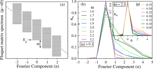
Figure 1: (a) Schematic spectrum of $\cal H$ for independent blocks $\mu\rightarrow 0$, where $E_{g}$ is the groundstate energy of $H_{0}$. (b) Norms of Fourier components ($\kappa_{n}=\||\Phi_{n}\rangle\|$) from Floquet DMRG simulations of Eq. (5) for different $\omega$ and different $\mu$ (inset) in units of $J$ using $N=30$.

Floquet DMRG – As in the original DMRG algorithm white92 ; scholl05 , in the first step a small system size is considered, so a desired eigenstate can be obtained exactly. In the static case the ground state can be found by standard Lanczos or Davidson methods, but for the Floquet matrix $\cal H$ in Eq. (3) this would result in a lowest quasi-energy state which is dominated by the largest possible Fourier component $M_{2}$ in Fig. 1a, which is not at all what we want since this situation corresponds to large truncation error. Instead the target state must be adiabatically connected to the ground state, which has the strongest weight in the $n=0$ sector in the middle of the quasi-energy spectrum in Fig. 1a. We therefore adopt the shift-and-square method with a dynamical shift. For diagonalization of the shifted and squared matrix $({\cal H}-\sigma\bm{1})^{2}$, we use Davidson’s algorithm davidson75 suitably modified for the present problem. The matrix $({\cal H}-\sigma\bm{1})^{2}$ is first projected onto a small search space, where the shift $\sigma$ takes the groundstate energy $E_{g}$ as its initial value. The small projected matrix is then fully solved and its eigenstate with largest overlap with the groundstate is picked up. This gives the first approximation of the desired eigenstate of $\cal H$, which in turn is used, by the correction vector method prescribed by Davidson, to enlarge the search space and then the whole process is repeated for this larger space. If the search space becomes inconveniently large, we restart the iterative process with the latest solution and replace the shift $\sigma$ by the approximate quasi-energy found at this stage (see Appendix for more details). Although $\cal H$ in Eq. (3) is a big matrix, it is possible to simplify the calculation by only manipulating smaller matrices $H_{0}$ and $H_{1}$.

We are now in the position to apply the DMRG algorithm, which is based on defining a suitable reduced density matrix from the previously targeted eigenstate, so that the basis set can be projected to the most important states before the system is enlarged white92 ; scholl05 . Since the steady state solution $|\Psi(t)\rangle$, all Fourier components $|\Phi_{n}\rangle$ as well as the static ground state are described by the same Hilbert space, we seek a suitable DMRG procedure, which projects all blocks in Eq. (3) simultaneously by the same transformation. Therefore the DMRG projection is found by truncating the original Hilbert space in the same way as in the static case, albeit using a different Floquet target state and corresponding reduced density matrix.

To illustrate the choice of density matrix for a given Floquet eigenstate $|\Psi(t)\rangle=e^{-i\epsilon t}\sum_{n=-\infty}^{\infty}e^{-in\omega t}|\Phi_{n}\rangle$, we write the Hilbert space as the product of two parts – system “S” and environment “E” – and consider the calculation of the time average of a local operator $A_{S}\otimes I_{E}$ acting on the system block “S”, where $I_{E}$ is the identity operator for the environment block “E”

$$\bar{A}_{S}=\frac{1}{T}\int_{0}^{T}\langle\Psi(t)|A_{S}\otimes I_{E}|\Psi(t)\rangle dt=Tr\{\rho_{F}A_{S}\}.$$ (4)

Here $\rho_{F}=\sum_{n=-\infty}^{\infty}\theta_{n}\rho_{n}$ and $\rho_{n}$ is the reduced density matrix of the block “S” for the normalized Fourier component $\frac{1}{\sqrt{\theta_{n}}}|\Phi_{n}\rangle$ with $\theta_{n}=\langle\Phi_{n}|\Phi_{n}\rangle$. Due to the normalization of a Floquet mode, $\sum_{n=-\infty}^{\infty}\theta_{n}=1$, $\rho_{F}$ will have properties of a density matrix. In particular, if $\rho_{F}|r_{i}\rangle=r_{i}|r_{i}\rangle$, then $r_{i}\geq 0$ and $\sum_{i=1}^{D_{S}}r_{i}=1$ where $D_{S}$ is the dimension of the state space of “S”.

Since we need the information of the groundstate of $H_{0}$ to find the Floquet target state, it is necessary to also consider the reduced density matrix of the groundstate $\rho_{G}$ in a linear combination $\rho=\lambda\rho_{F}+(1-\lambda)\rho_{G}$, which is then used in the renormalization. Here $0<\lambda<1$ and its optimal value can depend on the parameter regime we are working in. For low values of $\omega$ and large $|\mu|$, $\lambda$ plays a significant role. We find that the value of $\lambda=3/4$ gives a good balance between $\rho_{F}$ and $\rho_{G}$ in this regime. For larger frequencies the results become insensitive to the value of $\lambda$ since $\rho_{F}$ and $\rho_{G}$ are very close, so we keep $\lambda=3/4$ in all calculations.

In summary we have achieved the following Floquet DMRG procedure for the steady state eigenvalue problem: (i) For a small system (e.g. 6 sites), form $H_{0}$, $H_{1}$, and $\cal H$ in Eqs. (1) and (3) keeping finite number of Fourier modes ($M_{2}>M_{1}$). (ii) Find the static groundstate vector and energy of $H_{0}$. (iii) Find the Floquet mode with largest overlap with the groundstate, i.e. the eigenstate of $\cal H$ following the shift-and-square method described above. (iv) Divide the full system into two blocks – “S” and “E” (full system = $SE$). Form the reduced density matrix $\rho=\lambda\rho_{F}+(1-\lambda)\rho_{G}$ for “S” from the Floquet mode and the ground state. Diagonalize $\rho$ and retain $M$ most significant eigenvectors to project the relevant operators of “S” and “E” into this subspace. (v) Enlarge the system by adding two sites between the two blocks (new full system = $S\bullet\bullet E$). Form $H_{0}$ and $H_{1}$ for the extended system (“superblock”) to construct the corresponding $\cal H$. (vi) Go to the step (ii) and repeat until the system size reaches the target size. In all our simulations we use $M_{1}=3$, $M_{2}=5$, and $M=180$, giving a total superblock dimension of $4M^{2}(M_{1}+M_{2}+1)\gtrsim 10^{6}$ for the Floquet matrix $\cal H$, which is somewhat smaller than in ordinary DMRG calculations due to the more involved search algorithm for the target state in the middle of the spectrum.

Results – Using the Floquet DMRG method we study both locally (edge) and globally driven spin-1/2 Heisenberg antiferromagnetic chains (isotropic) with $N$ spins

$$H_{ld}(t) =J\sum_{i=1}^{N-1}\vec{S}_{i}\cdot\vec{S}_{i+1}+2\mu~{}\textrm{cos}(\omega t)S_{1}^{z}~{}~{}\textrm{and}$$ (5)

$$H_{gd}(t) =J\sum_{i=1}^{N-1}\vec{S}_{i}\cdot\vec{S}_{i+1}+2\sum_{j=1}^{N}\mu_{j}~{}\textrm{cos}(\omega t)S_{j}^{z}.$$ (6)

Here $\vec{S}_{i}$ is the $i^{\text{th}}$ spin and $S_{j}^{z}$ is the $z$-component of the $j^{\text{th}}$ spin. In Eq. (6) an incommensurate modulation is applied with $\mu_{j}=\mu\,\textrm{cos}~{}2\pi\beta j$ for $j\leq N/2$ and $\mu_{j}=\mu\,\textrm{cos}~{}2\pi\beta(N+1-j)$ for $j>N/2$ using $\beta=211/311$ in order to produce a dynamical pseudo-disorder for the globally driven system.

For comparison an effective high frequency model can be derived based on the exact solution of the corresponding Ising model without spin-flip with Ising eigenstates $|\{{s_{j}^{z}}\}\rangle=\prod_{\otimes j}|{s_{j}^{z}}\rangle$ where $|s_{j}^{z}\rangle$ represent the local $s_{j}^{z}$-basis states. The Floquet modes can then be exactly determined to be (see Appendix)

$$|\Phi(t)\rangle=\prod_{\otimes j}e^{-i\frac{2\mu_{j}}{\omega}s_{j}^{z}\sin(\omega t)}|s_{j}^{z}\rangle$$ (7)

with quasi-energies $\epsilon(\{s_{j}^{z}\})=J\sum_{j}s_{j}^{z}s_{j+1}^{z}$ in terms of $s_{j}^{z}$ quantum numbers. The Fourier decomposition in Eq. (2) yields $|\Phi_{n}\rangle=J_{-n}\left(\frac{2}{\omega}\sum_{j}\mu_{j}s_{j}^{z}\right)\prod_{\otimes j}|s_{j}^{z}\rangle,$ where $J_{n}(x)$ denote Bessel functions of the first kind. An effective static Hamiltonian is then derived in a high frequency approximation $\omega\gg J$ eckardt15 ; itin15 ; wang14 ; rahav03 by perturbatively calculating the time-averaged matrix elements of the full Floquet Hamiltonian $(H(t)-i\partial_{t})$ with respect to the Ising Floquet modes in Eq. (7) and taking into account only terms in the $n=0$ sector (see Appendix)

$$H_{\rm eff}=\sum_{j=1}^{N-1}\left[{J_{j,j+1}}\!\left(S^{x}_{j}S^{x}_{j+1}\!+\!S^{y}_{j}S^{y}_{j+1}\right)+JS^{z}_{j}S^{z}_{j+1}\right]$$ (8)

where $J_{j,j+1}=JJ_{0}\left(\frac{2(\mu_{j}-\mu_{j+1})}{\omega}\right)$. The comparison with this effective model allows a systematic analysis of the effect of higher Fourier modes on correlations in DMRG as the frequency is lowered.

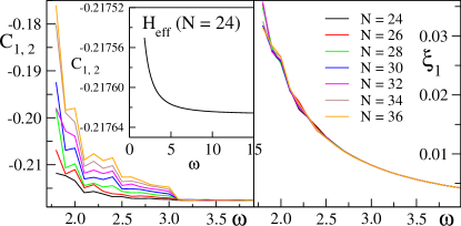
Figure 2: Floquet DMRG results for the correlations and fluctuations of the edge driven Heisenberg model in Eq. (5) for $\mu=0.1J$. The correlation result for the static effective Hamiltonian.

We first consider the locally driven model in Eq. (5) using the Floquet DMRG. Lowering the frequency from $\omega/J=3.2$ to $1.6$ we observe a significant occupation in higher Fourier components in Fig. 1b. This signals a rather sudden crossover from a high frequency regime described by Eq. (8) to a Floquet regime. This is also reflected in the spin correlations

$$C_{i,j}=\frac{1}{T}\int_{0}^{T}\langle\Phi(t)|S_{i}^{z}S_{j}^{z}|\Phi(t)\rangle dt$$ (9)

As shown in Fig. 2 (inset) for $C_{1,2}$ the effective model in Eq. (8) predicts a reduction of only 0.03% over this frequency range for $\mu=0.1J$ while the DMRG shows already a 100 times larger change for $N=24$. Moreover, the edge correlation $C_{1,2}$ shows a surprisingly strong dependence on site number $N$, which is well beyond conventional renormalization scenarios affleck ; rommer . The unexpected length dependence is caused by the reduced level spacing with increasing $N$, which facilitates a coupling and hybridization with an exponentially increasing number of higher energy states schneider for this parameter range. The spin fluctuation $\xi_{1}=\sqrt{[}\frac{1}{T}\int_{0}^{T}(\langle s_{1}^{z}(t)\rangle-\overline{s}_{1}^{z})^{2}dt]$ also increases quickly with lowered frequency as shown in Fig. 2, but does not show the same dramatic dependence on $N$. The accuracy of the DMRG, the dependence on states kept $M$, the overlap with the ground state, as well as the behavior of the quasi-energy $\epsilon-E_{g}$ are discussed in the Appendix.

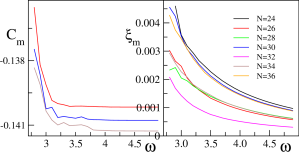
Figure 3: Floquet DMRG results for the correlations and fluctuations in the middle (m) of the bulk pseudo-randomly driven Heisenberg model in Eq. (6) for $\mu=0.02J$.

We now turn to the pseudo-randomly driven system in Eq. (6) for $\mu=0.02J$. In this case, we consider the average correlations in the middle (m) of the chain ${C}_{\rm m}=\frac{1}{3}\sum_{i=N/2-1}^{N/2+1}C_{i,i+1}$ and their corresponding fluctuations ${\xi}_{\rm m}=\sqrt{[}\frac{1}{4}\sum_{i=N/2-1}^{N/2+2}\xi_{i}^{2}]$ in Fig. 3. Again we observe a very quick change below frequencies $\omega\lesssim 3J$, but the length dependence is much less dramatic in this case. Note, that the dependence on $N$ for high frequencies can be attributed to the slight shift in local values of $\mu_{j}$ due to the incommensurate modulation.

Conclusion – We have shown that time-periodically driven many-body systems can be treated by a specifically adapted Floquet DMRG method. The main technical difficulty is the targeting of a Floquet mode, which is adiabatically connected to the ground state, but has a quasi-energy in the middle of the Floquet spectrum. This problem can be tackled by using a shift-and-square method in combination with Davidsons algorithm. Overall this limits the number of states $M$ which can be kept in the Floquet DMRG procedure compared to static ground state problems, but the accuracy is still very good over a wide parameter range, which allows to determine the emergent many-body correlations directly in the infinite-time steady-state limit.

It must be emphasized that it is a priori unclear which many-body systems will show the most interesting Floquet-induced correlations or dynamic phase transitions. A reliable but straight-forward numerical method such as this Floquet DMRG will therefore help to identify and classify promising correlated models. To initiate the search we have chosen the most obvious and maybe oldest bethe prototypical model of a Heisenberg spin chain. Time periodic driving is applied at the edge as well as in the bulk with a pseudo random distribution. For the edge driven system deviations from the effective high-frequency regime quickly occur starting below $\omega\lesssim 3J$ as can be seen in the occupation of higher Fourier components in Fig. 1 and the drop in edge correlations in Fig. 2 with an unexpectedly strong dependence on $N$. The global pseudo-random driving also shows a significant low-frequency change starting at approximately the same frequency $\omega\lesssim 3J$. Increasing the amplitude $\mu$ will shift this cross-over frequency to slightly lower values, but as can be seen in the inset of Fig. 1b the effect of changing $\mu$ is overall less pronounced than a change in $\omega$.

While these results are interesting, they also still lack a better understanding which may be found by comparison to a broader range of other relevant many-body systems in the future. We therefore hope that the proposed Floquet DMRG will provide a valuable tool to deepen the understanding of emergent many-body correlations from time-periodic driving.

–

I Appendix

This Appendix provides additional data on the quasi-energies and the wave-function overlap, a detailed discussion of the algorithm to find the eigenstate of the Floquet matrix $\cal H$, details on the numerical performance and error as a function of $M$ of the proposed DMRG method, as well as the derivation of the effective Hamiltonian in the large frequency limit.

I.1 Change of quasi-energies and wave-function overlap

In addition to the correlations and number of occupied Floquet modes, it is also interesting to consider the change of quasi-energies relative to the groundstate energy $\Delta=\epsilon_{q}-E_{g}$ and the magnitude of the wave-function overlap with the ground state $O_{g}=|\langle\psi_{g}|\Phi_{0}\rangle|$ as a function of frequency as shown in Fig. S1. The data shows a rather sudden change for $O_{g}$ as the frequency is lowered, fully consistent with the findings in the main text.

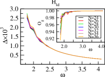
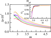
Figure S1: Overlap with the ground state $O_{g}$ and difference of the quasi-energy to the ground state energy $\Delta$ as a function of frequency for the edge driven and the globally driven model for different $N$.

I.2 Steady state solution: Finding the eigenstate of $\cal H$

We here adopt a projective method, similar to the standard Rayleigh-Ritz method, for solving $K=({\cal H}-\sigma\bm{1})^{2}$. First we consider a suitable search space $\mathcal{V}_{m}=\{v_{1},v_{2},\cdots,v_{m}\}$ of $m$ orthonormal vectors, where $m$ is much smaller than the actual dimension $d=4M^{2}(M_{1}+M_{2}+1)^{2}$ of the superblock for the truncated ${\cal H}$. The next step is to project $K$ onto this search space: $\tilde{K}_{m}=V_{m}^{\dagger}KV_{m}$, where $V_{m}$ is the projection matrix whose $i^{\text{th}}$ column is the vector $v_{i}$. In practice, to form the matrix $\tilde{K}_{m}$, we first get the new vectors $w_{i}$’s by applying $({\cal H}-\sigma\bm{1})$ to the vectors $v_{i}$’s: $w_{i}=({\cal H}-\sigma\bm{1})v_{i}$. Now the $ij^{\text{th}}$ element of $\tilde{K}_{m}$ is just the following inner product: $(\tilde{K}_{m})_{ij}=w_{i}^{\dagger}w_{j}$. Any full diagonalization routine can be used to solve the small projected matrix $\tilde{K}_{m}$. Let $z$ be one of its eigenvectors. Then, at this stage, the corresponding vector, called the Ritz vector, $V_{m}z$ is the best approximation of an eigenvector of $K$. Now after forming all the Ritz vectors ($m$ in number), we pick up the one which has time-averaged maximum overlap with the groundstate. Let $\Phi_{ov}$ be the approximate targeted Floquet mode obtained at this stage. The corresponding approximate quasi-energy is given by $\epsilon_{q}=\sigma+\Phi_{ov}^{*}({\cal H}-\sigma\bm{1})\Phi_{ov}$. This approximate eigenstate $\Phi_{ov}$ can now be improved by enlarging the search space $\mathcal{V}_{m}$ iteratively until we reach convergence. The enlargement is done by adding a new linearly independent vector $v_{m+1}$ to form the new search space $\mathcal{V}_{m+1}$ of dimension $m+1$. A common choice of $v_{m+1}$ is the correction vector, derived from the approximate eigenstate, as suggested by Davidson davidson75 . Let $r$ be the eigenvalue of the projected matrix $\tilde{K}_{m}$ corresponding to the vector $\Phi_{ov}$. Then the correction vector $C$ is defined as $C_{i}=[(K-r)\Phi_{ov}]_{i}/(r-K_{ii})$, where $K_{ii}$ is the $i^{\text{th}}$ diagonal element of the matrix $K$. This vector $C$ is then orthonormalized with the existing basis vectors of $\mathcal{V}_{m}$ to form the new basis vector $v_{m+1}$. After this, we construct the new projected matrix $\tilde{K}_{m+1}$ (this time we only need to calculate the elements corresponding to the new basis vector). The enlarged matrix $\tilde{K}_{m+1}$ is then diagonalized and the targeted mode is obtained from the appropriate eigenvector of the matrix. This iterative process is continued until the convergence is reached. If the dimension of the search space becomes inconveniently large (say, about 40), we restart the whole process with a few (say, about 10) latest approximate eigenstates which have largest overlap with the groundstate. During the restart, we also replace the scaling/shifting energy $\sigma$ by the approximate quasi-energy found at this stage. We found that this change in scaling energy makes the overall convergence much faster.

It may be worth mentioning here that, since we are looking for a Floquet mode with largest overlap with the groundstate, we begin the diagonalization process with just one vector $v_{1}=(\cdots,\psi_{g},\cdots)^{T}$, where the groundstate $\psi_{g}$ is placed in the block corresponding to $n=0$ Fourier component while all other elements are taken to be 0.

I.3 Performance of the proposed Floquet DMRG method

To verify the performance of the Floquet DMRG method, we first compare the Floquet DMRG results (quasi-energies) with the exact diagonalization (ED) results for system sizes N = 20 and 22. For the ED calculations, we solve the truncated ${\cal H}$ directly using the algorithm described above. For the Floquet DMRG calculations, we start with system size $N=6$ and then grow the system following the Floquet DMRG algorithm stated in the main text. The results can be seen in the Table 1 for both $H_{ld}$ and $H_{gd}$, where $\epsilon_{q}^{ED}$ ($\epsilon_{q}$) is the quasi-energy of the Floquet mode with largest ground-state overlap as found using ED (DMRG) method. To compare the quasi-energies relative to the corresponding groundstate energies $E_{g}$, the latter quantities are also provided in the Table. For representative parameter values, the accuracy in calculating the quasi-energies is found to be of the order of $10^{-7}$.

	$E_{g}$	$\epsilon_{q}^{ED}$	$|\epsilon_{q}^{ED}-\epsilon_{q}|$
$H_{ld}$(N=20)	-8.68247333	-8.68189932	$1.1\times 10^{-7}$
$H_{ld}$(N=22)	-9.56807587	-9.56750213	$1.2\times 10^{-7}$
$H_{gd}$(N=20)	-8.68247333	-8.68216072	$1.1\times 10^{-7}$
$H_{gd}$(N=22)	-9.56807587	-9.56773125	$5.2\times 10^{-7}$

Table 1: The calculations are done with $M_{1}=3$, $M_{2}=5$, and $m=180$. For $H_{ld}$, we take $\mu=0.1J$ and $\omega=3J$, and for $H_{gd}$, we take $\mu=0.02J$ and $\omega=3.5J$.

It may be stressed here that finding the Floquet mode by solving ${\cal H}$ does not follow the variational principle; as a consequence, the accuracy of a calculated quantity does not always increase monotonically with $M$ (maximum number of states retained at each Floquet DMRG step). However, overall results get better with increasing $M$, as can be seen in Fig. S2.

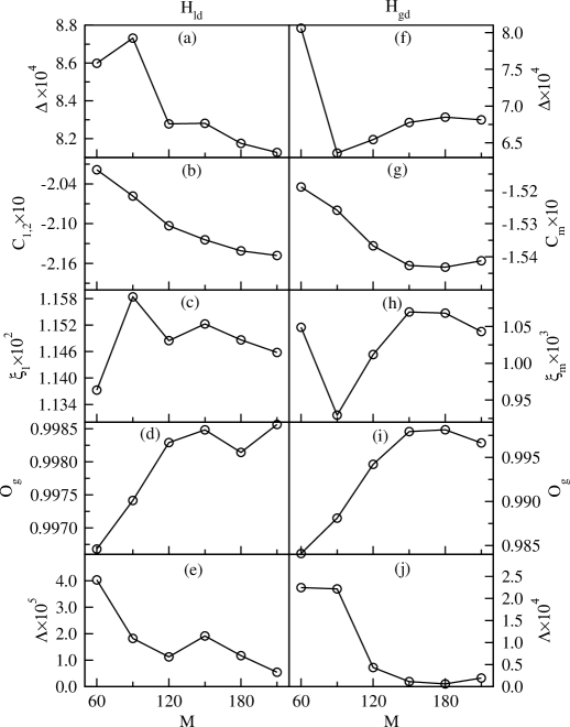
Figure S2: Different quantities for $N=32$ are plotted as function of $M$ for edge and globally driven systems in (a)-(e) and (f)-(j), respectively. We take $\omega=2.6J$ and $\mu=0.1J$ for the edge driven system $H_{ld}$, and $\omega=3.2J$ and $\mu=0.02J$ for the globally driven system $H_{gd}$.

For the locally driven system $H_{ld}$, the difference of the quasi-energy from the groundstate energy $\Delta=\epsilon_{q}-E_{g}$, the time-averaged correlation between the first two sites $C_{1,2}$, the temporal fluctuation of the first site $\xi_{1}$, the time-averaged overlap $O_{g}$ of the targeted mode with the groundstate and the DMRG truncation error $\Lambda$ are shown respectively in Fig. S2 (a) to (e). For the globally driven system $H_{gd}$, we show the same plots in Fig. S2 (f)-(j), except that this time we plot the average nearest-neighbor correlation ${C}_{m}$ and the average temporal fluctuation ${\xi}_{m}$ in the middle (m) instead of $C_{1,2}$ and $\xi_{1}$ respectively.
In the following, we estimate the error associated with the DMRG calculations (for $M=180$; since we obtained our main results keeping $M=180$). Let $A_{150}$, $A_{180}$ and $A_{210}$ are values of a quantity $A$ when we keep $M$ = 150, 180 and 210 respectively; then the average change in $A$ due to change in $M$ by 30 is $\frac{1}{2}(|A_{180}-A_{150}|+|A_{210}-A_{180}|)$. In each DMRG step the total system is enlarged by two spins, so that each block (E and S) has size $2M$, which is then again reduced to the $M$ states with the largest density matrix eigenvalues (discarding the other $M$ states). The relative error for discarding $M=180$ states can then be estimated from $\frac{1}{2}(|A_{180}-A_{150}|+|A_{210}-A_{180}|)\times\frac{180}{30}$. Accordingly for the locally driven system, the errors for the quantities $\epsilon_{q}$, $C_{1,2}$, $\xi_{1}$ and $O_{g}$ are estimated to be 3.32$\times 10^{-4}\%$, 3.33%, 1.69% and 0.23% respectively. Similarly for the globally driven system, the error estimations are 2.34$\times 10^{-4}\%$, 0.47%, 7.49% and 0.51% respectively for the quantities $\epsilon_{q}$, ${C}_{m}$, ${\xi}_{m}$ and $O_{g}$. It may be mentioned here that, to verify the performance of the DMRG method, we deliberately chose $\omega$ values in the intermediate/ moderate range (where system goes from the high-frequency localized phase to the low-frequency ergodic phase). The accuracy of a calculated quantity gets better as we move towards a high-frequency regime.

I.4 Derivation of the effective time-independent Hamiltonian

Let us consider the general periodically driven time-dependent Hamiltonian

$$H(t) =J\sum_{j=1}^{N-1}\left[\frac{1}{2}\left(S^{+}_{j}S^{-}_{j+1}+S^{-}_{j}S^{+}_{j+1}\right)+S^{z}_{j}S^{z}_{j+1}\right]+2\sum_{j=1}^{N}\mu_{j}~{}\textrm{cos}(\omega t)S^{z}_{j}.$$ (S1)

Its steady-state solution is of the form $|\psi(t)\rangle=e^{-i\epsilon t}\,|\Phi(t)\rangle$ where $|\Phi(t)\rangle=|\Phi(t+T)\rangle$ is time-periodic in $T=\frac{2\pi}{\omega}$ and fulfills the eigenvalue equation

$$\left(H(t)-i\frac{\partial}{\partial t}\right)|\Phi(t)\rangle=\epsilon|\Phi(t)\rangle.$$ (S2)

In solving Eq. (S2) in the large $\omega/\mu$ limit we follow the lines of Ref. wang14, . We first consider the simplified Hamiltonian

$$H_{0}(t) =J\sum_{j=1}^{N-1}S^{z}_{j}\cdot S^{z}_{j+1}+2\sum_{j=1}^{N}\mu_{j}~{}\textrm{cos}(\omega t)S^{z}_{j}$$ (S3)

which is diagonal in the Ising states $|\{{s_{j}^{z}}\}\rangle=\prod_{\otimes j}|{s_{j}^{z}}\rangle$. Here, $|s_{j}^{z}\rangle_{j}$ represents the local $S^{z}_{j}$-basis state, i.e. $S_{j}^{z}|s_{j}^{z}\rangle=s_{j}^{z}|s_{j}^{z}\rangle$. Consequently, the corresponding simplified Floquet equation

$$\left(H_{0}(t)-i\frac{\partial}{\partial t}\right)|\Phi(t)\rangle=\epsilon|\Phi(t)\rangle$$ (S4)

can be directly solved yielding solutions

$$|\Phi^{\ell}(t)\rangle=e^{i\ell\omega t}\prod_{\otimes j}e^{-i\frac{2\mu_{j}}{\omega}s_{j}^{z}\sin(\omega t)}|s_{j}^{z}\rangle$$ (S5)

and quasi-energies

$$\epsilon_{\ell}=J\sum_{j}s_{j}^{z}s_{j+1}^{z}+\ell\omega.$$ (S6)

Note, that we used the (trivial) index $\ell$ to extend the solutions over all values of $\epsilon$ analogous to the extended zone scheme for Bloch waves, which will later allow us to calculate matrix elements of solutions from different Floquet bands labeled by $\ell$. However, the physical relevant steady state solution $|\Phi(t)\rangle=|\Phi^{0}(t)\rangle$ corresponds to $\ell=0$ in Eq. (S5). Next, we take the non-diagonal spin-flip terms into account. For the effective Hamiltonian, we are interested in the time-averaged behavior. Therefore, we define the time-averaged scalar product

$$\langle\langle u_{1}(t)|u_{2}(t)\rangle\rangle=\frac{1}{T}\int_{0}^{T}dt\langle u_{1}(t)|u_{2}(t)\rangle$$ (S7)

and determine the corresponding matrix elements of the full Floquet Hamiltonian with respect to any two Floquet states $\Phi^{\ell_{1}}_{1}$ and $\Phi^{\ell_{2}}_{2}$ defined in Eq. (S5) in any Floquet bands, i.e.

$$\mathcal{H}_{\Phi_{1}^{\ell_{1}},\Phi^{\ell_{2}}_{2}}:=\langle\langle\Phi^{\ell_{1}}_{1}|\left(H(t)-i\frac{\partial}{\partial t}\right)|\Phi^{\ell_{2}}_{2}\rangle\rangle.$$ (S8)

We obtain in terms of the respective quantum-numbers ($\{s_{j}^{z}\}_{1}$ and $\{s_{j}^{z}\}_{2}$)

$$\mathcal{H}_{\Phi_{1}^{\ell_{1}},\Phi^{\ell_{2}}_{2}}=\langle\langle\Phi_{1}^{\ell_{1}}|\sum_{i}\frac{1}{2}\left(S^{+}_{i}S^{-}_{i+1}+S^{-}_{i}S^{+}_{i+1}\right)|\Phi^{\ell_{2}}_{2}\rangle\rangle+\delta_{\ell_{1},\ell_{2}}\delta_{\{s_{j}^{z}\}_{1},\{s_{j}^{z}\}_{2}}\epsilon_{\ell_{1}}.$$ (S9)

Note that the non-diagonal contributions $\langle\langle\Phi_{1}^{\ell_{1}}|S^{+}_{i}S^{-}_{i+1}|\Phi^{\ell_{2}}_{2}\rangle\rangle$ are only non-zero if $\{s_{j}^{z}\}_{1}=\{s_{j}^{z}\}_{2}$ for $j\neq i,i+1$ and $\{s_{i}^{z}\}_{1}=\{s_{i}^{z}\}_{2}+1$ and $\{s^{z}_{i+1}\}_{1}=\{s^{z}_{i+1}\}_{2}-1$. The corresponding phase factors are

$$\frac{1}{T}\int_{0}^{T}dt\;e^{i(\ell_{2}-\ell_{1})\omega t}e^{i\frac{2(\mu_{i}-\mu_{i+1})}{\omega}\sin(\omega t)}=J_{\ell_{2}-\ell_{1}}\left(\frac{2(\mu_{i}-\mu_{i+1})}{\omega}\right)$$ (S10)

where $J_{\ell}(z)$ denotes the Bessel function of the first kind. Taking into account only terms with $\ell_{1}=\ell_{2}$ is justified in the high frequency limit and gives the effective time-independent Hamiltonian

$$H_{\rm eff} =\sum_{j=1}^{N-1}\left[\frac{J_{j,j+1}}{2}\left(S^{+}_{j}S^{-}_{j+1}+S^{-}_{j}S^{+}_{j+1}\right)+JS^{z}_{j}S^{z}_{j+1}\right]$$ (S11)

with $J_{j,j+1}=JJ_{0}\left(\frac{2(\mu_{j}-\mu_{j+1})}{\omega}\right)$.

References

- (1) Y. Kayanuma and K. Saito, Coherent destruction of tunneling, dynamic localization, and the Landau-Zener formula, Phys. Rev. A 77, 010101(R) (2008).
- (2) T. Nag, S. Roy, A. Dutta, and D. Sen, Dynamical localization in a chain of hard core bosons under periodic driving, Phys. Rev. B 89, 165425 (2014).
- (3) M. Grifoni and P. Hänggi, Driven quantum tunneling, Phys. Rep. 304, 229 (1998).
- (4) Z. Cherpakova, C. Jörg, C. Dauer, F. Letscher, M. Fleischhauer, S. Eggert, S. Linden, and G. von Freymann, Limits of topological protection under local periodic driving, Preprint arXiv:1807.02321 (2018).
- (5) T. Prosen and E. Ilievski, Nonequilibrium Phase Transition in a Periodically Driven XY Spin Chain, Phys. Rev. Lett. 107, 060403 (2011).
- (6) T. Shirai, T. Mori, and S. Miyashita, Novel symmetry-broken phase in a driven cavity system in the thermodynamic limit, J. Phys. B: At. Mol. Opt. Phys. 47, 025501 (2014).
- (7) D. Thuberg, S.A. Reyes, and S. Eggert, Quantum resonance catastrophe for conductance through a periodically driven barrier, Phys. Rev. B 93, 180301(R) (2016).
- (8) S.A. Reyes, D. Thuberg, D. P rez, C. Dauer, and S. Eggert, Transport through an AC-driven impurity: Fano interference and bound states in the continuum, New J. Phys. 19, 043029 (2017).
- (9) D. V. Else, B. Bauer, and C. Nayak, Floquet Time Crystals, Phys. Rev. Lett. 117, 090402 (2016).
- (10) J. Zhang, P. W. Hess, A. Kyprianidis, P. Becker, A. Lee, J. Smith, G. Pagano, I.-D. Potirniche, A. C. Potter, A. Vishwanath, N. Y. Yao, and C. Monroe, Observation of a discrete time crystal, Nature 543, 217 (2017).
- (11) S. Choi, J. Choi, R. Landig, G. Kucsko, H. Zhou, J. Isoya, F. Jelezko, S. Onoda, H. Sumiya, V. Khemani, C. von Keyserlingk, N. Y. Yao, E. Demler, and M. D. Lukin, Observation of discrete time-crystalline order in a disordered dipolar many-body system, Nature 543, 221 (2017).
- (12) A.J. E. Kreil, H. Yu. Musiienko-Shmarova, D.A. Bozhko, A. Pomyalov, V. S. L’vov, S. Eggert, A. A. Serga, and B. Hillebrands, Tunable space-time crystal in room-temperature magnetodielectrics, Preprint arXiv:1811.05801.
- (13) V. Khemani, A. Lazarides, R. Moessner, and S.L. Sondhi, Phase Structure of Driven Quantum Systems, Phys. Rev. Lett. 116, 250401 (2016).
- (14) F. Görg, M. Messer, K. Sandholzer, G. Jotzu, R. Desbuquois, and T. Esslinger, Enhancement and sign change of magnetic correlations in a driven quantum many-body system, Nature 553, 481 (2018).
- (15) T. Wang, S. Hu, S. Eggert, A. Pelster, and X.-F. Zhang, Floquet-Induced Superfluidity with Periodically Modulated Interactions of Two-Species Hardcore Bosons in a One-dimensional Optical Lattice, Preprint arXiv:1807.00015 (2018).
- (16) M. S. Rudner, N. H. Lindner, E. Berg, and M. Levin, Anomalous Edge States and the Bulk-Edge Correspondence for Periodically Driven Two-Dimensional Systems, Phys. Rev. X 3, 031005 (2013).
- (17) N. Goldman and J. Dalibard, Periodically Driven Quantum Systems: Effective Hamiltonians and Engineered Gauge Fields, Phys. Rev. X 4, 031027 (2014).
- (18) M. Thakurathi, A. A. Patel, D. Sen, and Amit Dutta, Floquet generation of Majorana end modes and topological invariants, Phys. Rev. B 88, 155133 (2013).
- (19) D. Thuberg, E. Munoz, S. Eggert, and S.A. Reyes, Perfect spin filter by periodic drive of a ferromagnetic quantum barrier, Phys. Rev. Lett. 119, 267701 (2017).
- (20) M. Mitrano, A. Cantaluppi, D. Nicoletti, S. Kaiser, A. Perucchi, S. Lupi, P. Di Pietro, D. Pontiroli, M. Riccò, S. R. Clark, D. Jaksch, and A. Cavalleri, Possible light-induced superconductivity in K3C60 at high temperature, Nature 530, 461 (2016).
- (21) A. Eckardt and E. Anisimovas, High-frequency approximation for periodically driven quantum systems from a Floquet-space perspective, New J. Phys. 17, 093039 (2015).
- (22) A.P. Itin and M.I. Katsnelson, Effective Hamiltonians for Rapidly Driven Many-Body Lattice Systems: Induced Exchange Interactions and Density-Dependent Hoppings, Phys. Rev. Lett. 115, 075301 (2015).
- (23) T. Wang, X.-F. Zhang, F. E. A. dos Santos, S. Eggert, and A. Pelster, Tuning the quantum phase transition of bosons in optical lattices via periodic modulation of the s-wave scattering length, Phys. Rev. A 90, 013633 (2014).
- (24) S. Rahav, I. Gilary, and S. Fishman, Effective Hamiltonians for periodically driven systems, Phys. Rev. A 68, 013820 (2003).
- (25) S. R. White, Density matrix formulation for quantum renormalization groups, Phys. Rev. Lett. 69, 2863 (1992).
- (26) U. Schollwöck, The density-matrix renormalization group, Rev. Mod. Phys. 77, 259 (2005).
- (27) D. Poletti and C. Kollath, Slow quench dynamics of periodically driven quantum gases, Phys. Rev. A 84, 013615 (2011).
- (28) D. M. Kennes, A. de la Torre, A. Ron, D. Hsieh, and A. J. Millis, Floquet Engineering in Quantum Chains, Phys. Rev. Lett. 120, 127601 (2018).
- (29) C. Zhang, F. Pollmann, S. L. Sondhi, and R. Moessner, Density-Matrix Renormalization Group study of Many-Body Localization in Floquet Eigenstates, Ann. Phys. (Berlin) 529, 1600294 (2017).
- (30) H. Sambe, Steady States and Quasienergies of a Quantum-Mechanical System in an Oscillating Field, Phys. Rev. A 7, 2203 (1973).
- (31) P. Hänggi, Quantum transport and dissipation (WILEY-VCH, 1988), chap. 5.
- (32) E. R. Davidson, The Iterative Calculation of a Few of the Lowest Eigenvalues and Corresponding Eigenvectors of Large Real-Symmetric Matrices, J. Comput. Phys. 17, 87 (1975).
- (33) S. Eggert and I. Affleck, Magnetic impurities in half-integer-spin Heisenberg antiferromagnetic chains, Phys. Rev. B 46, 10866 (1992).
- (34) S. Rommer and S. Eggert, Spin- and charge-density oscillations in spin chains and quantum wires, Phys. Rev. B 62, 4370 (2000); Impurity corrections to the thermodynamics in spin chains using a transfer-matrix DMRG method, Phys. Rev. B 59, 6301 (1999).
- (35) I. Schneider, A. Struck, M. Bortz, and S. Eggert, Local Density of States for Individual Energy Levels in finite Quantum Wires, Phys. Rev. Lett. 101, 206401 (2008).
- (36) W. Heisenberg, Zur Theorie des Ferromagnetismus, Z. Physik, 49, 619 (1928); H. Bethe, Zur Theorie der Metalle, Z. Physik, 71, 205 (1931).