Abstract.

Structural models that admit multiple reduced forms, such as game-theoretic models with multiple equilibria, pose challenges in practice, especially when parameters are set-identified and the identified set is large. In such cases, researchers often choose to focus on a particular subset of equilibria for counterfactual analysis, but this choice can be hard to justify. This paper shows that some parameter values can be more “desirable” than others for counterfactual analysis, even if they are empirically equivalent given the data. In particular, within the identified set, some counterfactual predictions can exhibit more robustness than others, against local perturbations of the reduced forms (e.g. the equilibrium selection rule). We provide a representation of this subset which can be used to simplify the implementation. We illustrate our message using moment inequality models, and provide an empirical application based on a model with top-coded data.

Key words: Counterfactual Analysis, Multiple Equilibria, Equilibrium Selection Rule, Locally Robust Refinement

JEL Classification: C30, C57

1. Introduction

Economists often use a structural model to analyze the effect of a policy that has never been implemented, such as potential mergers or changes to legislation. For such analysis, it is crucial to have a plausible specification of the causal relationship between the policy variable and the outcome variable of interest. However, a plausible specification can come short of determining the causal relationship uniquely. Prominent examples are found in game theoretic models, where the presence of multiple equilibria admits multiple reduced forms. (Tamer:03:ReStud called models with multiple reduced forms incomplete.) The multiplicity of reduced forms is often the source of set-identification of structural parameters.

When a parameter is set-identified, all the values in the identified set are empirically equivalent, in the sense that the observed data cannot be used to distinguish between the values. The identified set represents the empirical content of the model for the parameter (i.e., the amount of information on the value of the parameter that can be extracted from data through the model). However, when a parameter is set-identified with a large identified set, the identified set can be of little use for counterfactual analysis in practice. It is not unusual that predictions from counterfactual analysis based on different equilibria yield self-contradictory results (Aguirregabiria/Nevo:12:WP, p.111). In this situation, just as in the calibration approach in macroeconomics, the researcher typically uses additional constraints on the parameter values or chooses a specific equilibrium to obtain a meaningful analysis. In other words, the researcher considers a refinement of the identified set, by introducing additional restrictions. However, these restrictions are often only weakly motivated.

In our view, a desirable approach in this situation is to distinguish between the identification step and the refinement step, and lay out transparently what criterion (or motivation) is used for the refinement step. There is a small body of literature that explores this refinement step. Song:14:ET analyzed the problem of choosing a point from the identified interval based on the local asymptotic minimax regret criterion. Aryal/Kim:13:JBES considered an incomplete English auction model where the seller is ambiguity averse, and employing the $\Gamma$-maximin expected utility framework of Gilboa/Schmeidler:89:JME, suggested a point decision on the optimal reserve price. Jun/Pinkse:17:WPa considered an incomplete English auction set-up similar to that in Haile/Tamer:03:JPE and proposed a point decision on the optimal reserve price using a maximum entropy method. Jun/Pinkse:19:JOE studied a discrete two-player complete information game and established sharp identification of counterfactual predictions of the game. Furthermore, they investigated point decisions on the probability distributions through a maximum entropy method and what they called a Dirichlet approach, and compared the two methods.

The main goal of this paper is to draw attention to the fact that some values in the identified set can give counterfactual predictions that are more robust to the change of certain aspects of model specification than others. Thus, it is reasonable to give priority to those values that produce most “reliable” counterfactual predictions. Generally speaking, predictions that are sensitive to a change of the aspects of the model that the researcher is not sure about cannot be reliable. Given that the researcher is often least sure about how a reduced form is determined among multiple reduced forms, we consider a subset of the identified set which produces counterfactual predictions that are more robust to local perturbations of the reduced forms (e.g. local perturbations of the equilibrium selection rule in a game setting) than others.

More specifically, consider a causal relationship between endogenous variable $y$ and exogenous variables $x,\varepsilon$:

$$y=\rho_{\beta,\gamma}(x,\varepsilon;\eta),$$ (1.1)

where $\beta$ is the parameter of interest, $\gamma$ a nuisance parameter, and $\eta$ is a random variable with distribution $G$. Without observing $\eta$ or knowing $G$, the model admits multiple reduced forms. For example, in the case of games with multiple equilibria, $G$ plays the role of the equilibrium selection rule.

Suppose that the counterfactual setting of interest involves a counterfactual distribution $\tilde{F}_{X}$ for $X$. Consider the average structural function (ASF) (Blundell/Powell:04:ReStud):

$$\textsf{ASF}_{\beta,\gamma,G}(x)=\int\int\rho_{\beta,\gamma}(x,\varepsilon;\eta)dG(\eta|x,\varepsilon)dF_{\varepsilon}(\varepsilon),$$

where $F_{\varepsilon}$ denotes the distribution of $\varepsilon$, and $G(\cdot|x,\varepsilon)$ the conditional distribution of $\eta$ given $x$ and $\varepsilon$. Then our proposal is that we choose $\gamma$ that minimizes

$$\sup_{G^{\prime}\in B(G;\delta)}\left|\int\textsf{ASF}_{\beta,\gamma,G}(x)d\tilde{F}_{X}(x)-\int\textsf{ASF}_{\beta,\gamma,G^{\prime}}(x)d\tilde{F}_{X}(x)\right|,$$ (1.2)

where $B(G;\delta)$ denotes a $\delta$-neighborhood of $G$ for some small $\delta>0$. (As we show later, given $\beta$, the set of $\gamma$’s that minimize (1.2) does not depend on the choice of $\delta$ or $G$.) We call the resulting set of values $(\beta,\gamma)$ in the identified set the Locally Robust Refinement (LRR). In other words, our refinement is motivated by the desirability of a stable behavior in the counterfactual predictions when the structural parameters are partially identified.

In many set-ups, the LRR is a substantially smaller set than the identified set. Furthermore, the LRR is often very intuitive. For example, as we show in Section 3, the LRR in an entry game picks nuisance parameter values that minimize the region of multiple equilibria. In the example of a switching regression model with interval data, it picks nuisance parameters that minimize a difference across models in switching regression.

However, unlike the identified set, the size of the LRR does not indicate the empirical content of the model. Rather the LRR gives parameter values which produce counterfactual predictions that are most robust to the change of the reduced forms among their multiple forms. Due to this robustness property, one may want to pay more attention to those parameter values than others when conducting policy exercises, even if all the values in the identified set are observationally equivalent.

The formulation in (1.2) gives the impression that the LRR involves additional optimization over an infinite dimensional space in estimation, adding to computational cost. Using the linearity of $\textsf{ASF}_{\beta,\gamma,G}(x)$ in $G$ and Hilbert space geometry, this paper gives a simple characterization of the LRR so that focusing on the LRR does not cause extra computational cost. In fact, due to the additional constraints that come from the LRR, the computational cost is substantially reduced from a benchmark case without using the LRR. Focusing on moment inequality models, this paper presents a method of bootstrap inference on the LRR from the identified set and shows its uniform asymptotic validity. We provide results from Monte Carlo simulations, and illustrate the LRR through an empirical application on top-coded data. These exercises illustrate that the LRR’s predictions are indeed more stable than those with the identified set and that they may affect policymaking in applied contexts (i.e. policies suggested by the identified set could be driven by parameter values that are not robust, and are not part of the LRR).

There has long been interest in studying model sensitivity and robustness to misspecifications in econometric models. Recent contributions in this line include Andrews/Gentzkow/Shapiro:18:NBER, Armstrong/Kolesar:20:QE and Bonhomme/Weidner:20:WP who, among many others, proposed a method of measuring local misspecification and performing inference that is robust to local misspecifications. In the context of instrumental variable models, Nevo/Rosen:12:ReStat permitted the instrumental variable to be correlated with the error term and presented bounds for the parameter of interest under an assumption on the correlation between the instrumental variable and the error term. Oster:19:JBES proposed a method of extracting information on the omitted variable bias from data in linear regression models. Masten/Poirier:18:Ecma provided an identification analysis of various treatment effect parameters from treatment effect models where the conditional independence restriction is weakened to a partial dependence condition. Christensen/Connault:19:WP proposed a computationally tractable method of performing inference on counterfactual quantities that arise in structural models, while permitting a global misspecification of the model. Li:19:WP uses a semiparametric restriction (instead of parametric ones) to generate bounds for counterfactuals of interest in moment inequality models.

All these authors are concerned about robustness of inference to misspecifications. Their robust inference often leads to a larger confidence set, and a wider range of policy predictions. In contrast, we consider settings where the identified set is already too large to be useful for a meaningful policy analysis. This can happen even if the model is correctly specified (see Aguirregabiria/Nevo:12:WP for a discussion, particularly in the context of multiple equilibria). Instead of enlarging an existing identified set by “robustifying” it as above, we explore a rationale for focusing on a subset of the identified set for policy analysis. Our criterion is based on the stability of counterfactual predictions as we perturb the reduced-form selection rules. One can relate our guiding philosophy to the literature of equilibrium refinements in game theory, where one focuses on a subset of the set of Nash equilibria based on its stability against various perturbations of the game. (See Chapter 5 of Myerson:91:GameTheory.) Then the idea of local robustness in the paper, i.e., the stability of reduced forms against local perturbations of reduced form selection rules is related to Fudenberg/Kreps/Levine:88:JET who considered robustification of the set of strict Nash equilibria against local perturbations of the games.

The paper is organized as follows. The next section gives a general set-up of a structural model and presents examples that fit our framework. Section 3 presents the approach of LRR and provides its characterization that is useful for implementation in practice. Focusing on generic moment inequality models, Section 4 proposes inference for the LRR and presents results from Monte Carlo simulations. An empirical application is presented in Section 5. Section 6 concludes. In the Appendix, we provide some mathematical proofs. The Supplemental Note to this paper includes additional information on the data for the empirical application, and presents results on the uniform validity of our inference procedure.

2. A Counterfactual Analysis with Multiple Reduced Forms

2.1. Models with Multiple Reduced Forms

Suppose that data $\{(Y_{i}^{\prime},X_{i}^{\prime})^{\prime}\}_{i=1}^{n}$ are drawn from the joint distribution $P$ of $(Y^{\prime},X^{\prime})^{\prime}$ which obeys the following reduced form: for $Y\in\mathbf{R}$ and $W=(X^{\prime},\varepsilon^{\prime})^{\prime}$,

$$Y=\rho(W;\eta),$$ (2.1)

for some function $\rho$, where $X$ is observed but $\varepsilon$ and $\eta$ are not. For each value $\eta$, we regard the map $\rho(\cdot;\eta)$ as representing a functional-causal relationship between internal variable $Y$ and external variables $W$. This relationship is fully determined once the value of $\eta$ is realized. Typically, $\varepsilon$ has a structural meaning such as unobserved costs, whereas $\eta$ does not and is used only as an index for a reduced form. For example, in a game-theoretic model, $W=(X^{\prime},\varepsilon^{\prime})^{\prime}$ represents observed and unobserved payoff components and $\eta$ an index for an equilibrium. The response of $Y$ to a change in $W$ is ambiguous unless the value of $\eta$ is fixed. In this sense, there is a multiplicity of reduced forms in (2.1). To describe the generation of observed outcome $Y$, we assume that Nature selects the value of $\eta$ from the conditional distribution $G(\cdot|w)$ given $W=w$. In a game setting, $G$ is often called the equilibrium selection rule. However, the multiplicity of reduced forms can arise in a setting that has nothing to do with a game, such as in the case of switching regressions with interval data which we describe below. Hence we call $G$ the reduced-form selection rule in this paper.

2.2. Counterfactual Analysis Under Partial Identification

We focus on a counterfactual experiment where the distribution $F$ of the external vector $W$ is changed to a counterfactual one $\tilde{F}$. Such a counterfactual experiment includes cases where one “shuts off” the effect of a certain covariate, “fixing” of the covariate to a certain value, or changing the distribution of $\varepsilon$. Suppose that the counterfactual quantity of interest is generically denoted by $C(\rho,\tilde{F},G)$. This quantity could be, for example, the prediction of game outcomes or expected payoffs under a counterfactual scenario:

$$C(\rho,\tilde{F},G)=\int\rho(w;\eta)dG(\eta|w)d\tilde{F}(w).$$

Or in other applications, $C(\rho,\tilde{F},G)$ could be the average increase in welfare. Let $\mathcal{G}$ be the space of the reduced-form selection rules $G$ and let $\mathcal{R}$ be the identified set for the function $\rho$. Then the identified set for the counterfactual prediction $C(\rho,\tilde{F},G)$ is given by

$$\{C(\rho,\tilde{F},G):G\in\mathcal{G},\rho\in\mathcal{R}\}.$$

A standard approach to make inference based on this identified set faces multiple challenges in practice. The set of predictions can be of little practical use, when the estimated set is too large. Furthermore, estimation of the identified set itself and statistical inference can be computationally intensive.

Due to these difficulties, it is not unusual that empirical researchers focus on a particular subset of $\mathcal{G}$ (such as focusing on a particular equilibrium) or consider a subset of $\mathcal{R}$ (such as by restricting the admissible values of parameters as in the case of calibration). Such a subset selection approach, while inevitable in practice, is not easy to motivate.

2.3. Examples

For brevity, we consider two examples here to illustrate our set-up: a finite game of complete information and a switching regression with interval data.

2.3.1. Finite Game of Complete Information

Consider the setting of a complete information $N$ player game with finite actions, and let $A$ be the finite action space for each player. Suppose that the payoff for player $i$ playing $\tilde{a}\in A$ when all other players are playing $a_{-i}=(a_{j})_{j\neq i}$ is given by $u_{i}(\tilde{a},a_{-i},W)$ for a map $u_{i}$, where $W=(X,\varepsilon)$ is a payoff-relevant characteristic vector of player $i$. For each $a\in A^{N}$, we define

$$\mathbb{W}(a)=\left\{w:u_{i}(a_{i},a_{-i},w)\geq\max_{a^{\prime}\in A}u_{i}(a^{\prime},a_{-i},w),\forall i=1,...,N\right\}.$$ (2.2)

Hence if $w$ belongs to $\mathbb{W}(a)$, $a$ is a Nash equilibrium for the game with $w$, so that the set

$$\mathcal{A}(w)=\left\{a\in A^{N}:w\in\mathbb{W}(a)\right\}$$ (2.3)

represents the set of equilibria for the game with $w$. Let $\eta$ be a random vector taking values in $A^{N}$ where the conditional distribution $G(\cdot|w)$ of $\eta$ given $w$ has a support in $\mathcal{A}(w)$. Let $Y=(Y_{i})_{i=1}^{N}$ be the observed action profile that comes from a Nash equilibrium $\eta$ of the game after Nature draws $\eta$ from $G(\cdot|w)$. Then, we can write for $i\in N$,

$$Y_{i}=\rho_{i}(W;\eta),$$ (2.4)

where $\rho_{i}$ is the $i$-th entry of $\rho$ which is defined as

$$\rho(w;\eta)=\sum_{a\in\mathcal{A}(w)}1\{\eta=a\}a.$$

The conditional distribution $G(\cdot|w)$ over $\eta$ represents the equilibrium selection rule.

2.3.2. A Switching Regression Model with Interval Outcomes

Consider an interval data set-up similar to one studied by Manski/Tamer:02:ECMA. More specifically, we consider top-coded data with threshold variables $Z_{1}<Z_{2}$, where $Z_{1},Z_{2}$ are observed and common across individuals. We observe an outcome random variable which equals a latent $Y$ if $Y\leq Z_{1}$ and is only known to be within $[Z_{1},Z_{2}]$ otherwise, and a vector of covariates $X_{1}$. For example, $X_{1}$ represents a vector of covariates for each worker such as age, education, experience, gender, and $Y$ is the log of the hourly wage.

It is assumed that the latent $Y$ follows:

$$Y=\left\{\begin{array}[]{ll}g_{1}\left(\beta_{0}D+X_{1}^{\prime}\gamma_{0}\right)+\varepsilon,&\text{ if }\eta=1,\text{ and }\\ g_{2}\left(\beta_{0}D+X_{1}^{\prime}\gamma_{0}\right)+\varepsilon,&\text{ if }\eta=0,\end{array}\right.$$

where $D$ denotes the policy variable, and $\eta$ the binary indicator of a regime, and $g_{1}$ and $g_{2}$ are some known functions. As for the error term $\varepsilon$, we assume that $\mathbf{E}[\varepsilon|X_{1},D]=0$. We also assume that $Y\leq Z_{2}$ with probability one. Let $\tilde{Y}_{1}=\tilde{Y}_{2}=Y$ if $Y\leq Z_{1}$, and $\tilde{Y}_{1}=Z_{1}$ and $\tilde{Y}_{2}=Z_{2}$ if $Y>Z_{1}$. The econometrician observes $\tilde{Y}_{1}$ and $\tilde{Y}_{2}$. Let $\pi_{0}(X_{1},D)=P\{\eta=1|X_{1},D\}$ and $\Pi$ be the collection of functions that $\pi_{0}$ is known to belongs to.

It is straightforward that the identified set for $(\beta_{0},\gamma_{0})$ is given by

$$\Theta_{P}=\left\{(\beta_{0},\gamma_{0}):\mathbf{E}[\tilde{Y}_{1}|X_{1},D]\leq\alpha(X_{1},D;\beta_{0},\gamma_{0},\pi)\leq\mathbf{E}[\tilde{Y}_{2}|X_{1},D],\text{a.e.}\text{ for some }\pi\in\Pi\right\},$$ (2.6)

where

$$\alpha(X_{1},D;\beta_{0},\gamma_{0},\pi)=g_{1}\left(\beta_{0}D+X_{1}^{\prime}\gamma_{0}\right)\pi(X_{1},D)+g_{2}\left(\beta_{0}D+X_{1}^{\prime}\gamma_{0}\right)(1-\pi(X_{1},D)).$$ (2.7)

Now we can write

$$Y=\rho(X,\varepsilon;\eta),$$

where $X=(X_{1},D)$, and

$$\rho(X,\varepsilon;\eta)=g_{1}\left(\beta_{0}D+X_{1}^{\prime}\gamma_{0}\right)\eta+g_{2}\left(\beta_{0}D+X_{1}^{\prime}\gamma_{0}\right)(1-\eta)+\varepsilon.$$ (2.8)

The distribution $G$ of $\eta$ plays a role analogous to the equilibrium selection rule in a game-theoretic model. Here it selects from a given set of reduced forms.

3. Locally Robust Refinement

3.1. Overview

Suppose that the reduced-form $\rho(\cdot;\eta)$ in (2.1) is parametrized as follows:

$$Y=\rho_{\beta_{0},\gamma_{0}}(W;\eta),$$ (3.1)

where $\beta_{0}$ is a parameter of interest taking values in a set $B$ and $\gamma_{0}$ is a nuisance parameter taking values in a set $\Gamma$, and $\eta$ belongs to some known compact set denoted by $H$. Let $\Theta_{P}$ be the identified set for $(\beta_{0},\gamma_{0})$. The counterfactual experiment involves changing the distribution $F$ of $W$ to a counterfactual distribution $\tilde{F}$. Let us consider the counterfactual average structural outcome:

$$\textsf{ASO}_{\beta_{0},\gamma_{0}}(G)=\int\int\rho_{\beta_{0},\gamma_{0}}(w;\eta)dG(\eta|w)d\tilde{F}(w).$$ (3.2)

This is the average value of outcome $Y$ when a counterfactual change is made to the distribution of $W$ while everything else remains the same. Our focus is on a subset of $\Theta_{P}$ at which $\textsf{ASO}_{\beta,\gamma}(G)$ behaves robustly as we perturb the reduced-form selection rule $G$.

More formally, for any $K>0$, we introduce a $K$-sensitivity of $\textsf{ASO}_{\beta,\gamma}(G)$ as we perturb $G$ around in its $K$-neighborhood:

$$S_{\beta,\gamma}(G;K)=\sup_{G^{\prime}\in\mathcal{G}:\delta_{\mathcal{G}}(G^{\prime},G)\leq K}\frac{|\textsf{ASO}_{\beta,\gamma}(G^{\prime})-\textsf{ASO}_{\beta,\gamma}(G)|}{\delta_{\mathcal{G}}(G^{\prime},G)},$$ (3.3)

where $\mathcal{G}$ denotes the collection of $G$’s permitted in the model. The quantity $S_{\beta,\gamma}(G;K)$ measures the maximal rate of change of counterfactual average outcome when $G$ is perturbed within its $K$-neighborhood, where this neighborhood is defined using a metric $\delta_{\mathcal{G}}(G^{\prime},G)$, formally defined below. We search for values of nuisance parameters $\gamma$ which minimize this sensitivity. For each $\beta\in B$, if we let

$$\Gamma^{\mathsf{LRR}}(\beta)=\text{argmin}_{\gamma:(\beta,\gamma)\in\Theta_{P}}S_{\beta,\gamma}(G;K),$$ (3.4)

we define

$$\Theta_{P}^{\mathsf{LRR}}=\{(\beta,\gamma)\in\Theta_{P}:\gamma\in\Gamma^{\mathsf{LRR}}(\beta)\}.$$ (3.5)

We call the subset $\Theta_{P}^{\mathsf{LRR}}$ the Locally Robust Refinement (LRR) of $\Theta_{P}$. Hence, the LRR can be viewed as a collection of parameters at which the ASO is stable against local misspecifications of $G$. As we will see later in the characterization of the LRR set, the set is independent of the choice of $K$, $G$ and $\mathcal{G}$. The main reason behind this independence is that the functional $\textsf{ASO}_{\beta,\gamma}(G)$ is linear in $G$. (This is analogous to that the slope of a linear function is constant on the domain of the function.) Note that, as we do not want our concern of local robustification against the reduced-form selection rules to directly affect the parameter of interest, our approach subjects only the nuisance parameters to the refinement.

The inference on $\beta$ based on the Locally Robust Refinement proceeds under the further restriction as follows.

$$(\beta_{0},\gamma_{0})\in\Theta_{P}^{\mathsf{LRR}}.$$ (3.6)

We call this restriction the LRR Hypothesis. Once we focus on the LRR set of parameters, this can be used for various exercises of counterfactual analysis, just as one does with the identified set of parameters. Despite the impression that finding the set $\Theta_{P}^{\mathsf{LRR}}$ might be computationally intensive as it involves layers of optimization, it is not, due to our characterization result in the next section.

3.2. Characterization of the Locally Robust Refinement

To derive a characterization of the LRR, let us introduce some geometric structure on the space of reduced-form selection rules $G$. Let $\mathcal{G}$ be the collection of all the conditional distributions $G$ (of $\eta$ given $W$) which are dominated by the uniform distribution $\mu$ over $H$, and $w\in\mathcal{W}$, with $\mathcal{W}$ denoting the set $W$ takes values from. Let us introduce the following metric on $\mathcal{G}$: for $G,G^{\prime}\in\mathcal{G}$,

$$\delta_{\mathcal{G}}(G^{\prime},G)=\sqrt{\int\int\left(\frac{dG^{\prime}}{d\mu}-\frac{dG}{d\mu}\right)^{2}(\eta|w)d\mu(\eta)d\tilde{F}_{P}(w)}.$$ (3.7)

Let us define

$$\Gamma(\beta)=\{\gamma\in\Gamma:(\beta,\gamma)\in\Theta_{P}\},$$ (3.8)

i.e., the set of nuisance parameters that are admitted in the counterfactual analysis together with given $\beta$. For $\kappa\geq 0$, we define the $\kappa$-LRR set for $\gamma$ corresponding to $\beta$ as

$$\quad\quad\Gamma_{\kappa}^{\mathsf{LRR}}(\beta)=\left\{\gamma\in\Gamma(\beta):S_{\beta,\gamma}^{2}(G;K)\leq S_{\beta,\tilde{\gamma}}^{2}(G;K)+\kappa,\forall\tilde{\gamma}\in\Gamma(\beta)\right\},$$ (3.9)

where $S_{\beta,\gamma}(G;K)$ is defined in (3.3). The set $\Gamma^{\mathsf{LRR}}(\beta)$ defined in (3.4) is a special case of $\Gamma_{\kappa}^{\mathsf{LRR}}(\beta)$ with $\kappa=0$. However, as we discuss in Section 4.1, it is convenient to use the LRR set with a small positive number $\kappa>0$ which allows us to develop uniform inference. As shown below, this set does not depend on the choice of $K>0$ or that of $G\in\mathcal{G}$.

We now provide a useful characterization of the set $\Gamma_{\kappa}^{\mathsf{LRR}}(\beta)$. For this, we define

$$\Delta_{\beta,\gamma}(w;\eta)=\rho_{\beta,\gamma}(w;\eta)-\int\rho_{\beta,\gamma}(w;\eta)d\mu(\eta).$$

The function $\Delta_{\beta,\gamma}(w;\eta)$ is a mean-deviation form of the structural function $\rho_{\beta,\gamma}(w;\eta)$. This function plays a central role in the characterization result. Let us make the following assumption that guarantees that the average variability of this mean-deviation is well defined.

Assumption 3.1.

For each $\beta\in B$ and $\gamma\in\Gamma(\beta)$, $Q^{\mathsf{LRR}}(\beta,\gamma)<\infty$, where

$$Q^{\mathsf{LRR}}(\beta,\gamma)=\int\int\Delta_{\beta,\gamma}^{2}(w;\eta)d\mu(\eta)d\tilde{F}(w).$$ (3.10)

In applications where we can compute $\rho_{\beta,\gamma}(w;\eta)$ for each value of $\eta$, we can evaluate $Q^{\mathsf{LRR}}(\beta,\gamma)$ easily. (See Section 3.3 below for examples.) The following theorem shows that the set $\Gamma_{\kappa}^{\mathsf{LRR}}(\beta)$ is fully characterized through the function $Q^{\mathsf{LRR}}(\beta,\gamma)$.

Theorem 3.1.

Suppose that Assumption 3.1 holds. Then for each $\beta\in B$ and $\gamma\in\Gamma(\beta)$,

$$S_{\beta,\gamma}(G;K)=\sqrt{Q^{\mathsf{LRR}}(\beta,\gamma)},$$ (3.11)

for all $G\in\mathcal{G}$ and all $K>0$.

Thus the $\kappa$-LRR of $\gamma_{0}$ can be rewritten as

$$\Gamma_{\kappa}^{\mathsf{LRR}}(\beta)=\left\{\gamma\in\Gamma(\beta):Q^{\mathsf{LRR}}(\beta,\gamma)\leq Q^{\mathsf{LRR}}(\beta,\bar{\gamma})+\kappa,\text{ for all }\bar{\gamma}\in\Gamma(\beta)\right\}.$$ (3.12)

The $\kappa$-LRR of the nuisance parameter vector $\gamma_{0}$ is the set of $\gamma$’s which minimize the average variability of $\rho_{\beta,\gamma}(w;\eta)$ (around its mean) as we perturb $\eta$. Thus, the $\kappa$-LRR for $(\beta_{0},\gamma_{0})$ is given by

$$\Theta_{\kappa,P}^{\mathsf{LRR}}=\left\{(\beta,\gamma)\in\Theta_{P}:\gamma\in\Gamma_{\kappa}^{\mathsf{LRR}}(\beta)\right\}.$$ (3.13)

Sometimes, the target parameter may not be a parameter $\beta$ that determines the reduced form $\rho_{\beta,\gamma}$ but some aggregate quantity such as Average Treatment Effects or aggregate welfare. Suppose that such a target parameter is identified up to $\beta_{0}$ and $\gamma_{0}$, so that we can write it as, say $\psi(\beta_{0},\gamma_{0})$. (We give an example in Section 3.3.2 below.) Then, the LRR set for $\psi(\beta_{0},\gamma_{0})$ is given by

$$\Psi_{\kappa}^{\mathsf{LRR}}=\left\{\psi(\beta,\gamma):(\beta,\gamma)\in\Theta_{\kappa,P}^{\mathsf{LRR}}\right\}.$$ (3.14)

To build familiarity with our characterization results for the LRR and show how it can be used in practice, we now derive $Q^{LRR}$ for two applied examples.

3.3. Examples

3.3.1. Entry Game with Nash Equilibria

Consider the setting of a 2x2 complete information entry games, such as the empirical setting in Bresnahan/Reiss:91:JOE and Ciliberto/Tamer:09:Eca, where there are two firms, $i=1,2$, deciding whether to enter a market or not. The entry decisions of the firms can then be formulated as

$$D_{1} =1\{\beta_{1,0}D_{2}+X^{\prime}\gamma_{1,0}\geq\varepsilon_{1}\},\text{ and }$$ (3.15)

$$D_{2} =1\{\beta_{2,0}D_{1}+X^{\prime}\gamma_{2,0}\geq\varepsilon_{2}\},$$ (3.16)

where $\beta_{1,0}D_{2}+X^{\prime}\gamma_{1,0}-\varepsilon_{1}$ represents the payoff difference for firm $1$ between entering and not entering the market, $D_{i}=1$ represents the entry decision by firm $i$ and $D_{i}=0$ the decision not to enter by firm $i$. The random vectors $X$ and $\varepsilon$ represent respectively the observed and unobserved characteristics of firms $1$ and $2$ combined. The coefficients $\beta_{1,0}$ and $\beta_{2,0}$ capture strategic interactions between firms and they are our coefficients of interest, whereas the coefficients $\gamma_{1,0}$ and $\gamma_{2,0}$ measure the roles of firm specific and market specific characteristics and, as such, are nuisance parameters.

[INSERT FIGURE 1 HERE]

In order to find a reduced form as in (2.1), we first put

$$Y=(D_{1},D_{2}),\text{ and }\varepsilon=(\varepsilon_{1},\varepsilon_{2}),$$

where $Y\in\mathcal{Y}=\{(0,0),(1,1),(0,1),(1,0)\}$. Define (with $\beta_{0}=(\beta_{1,0}^{\prime},\beta_{2,0}^{\prime})^{\prime}$ and $\gamma_{0}=(\gamma_{1,0}^{\prime},\gamma_{2,0}^{\prime})^{\prime}$)

$$A_{1,\beta_{0},\gamma_{0}}(X) =\{(e_{1},e_{2})\in\mathbf{R}^{2}:X^{\prime}\gamma_{1,0}<e_{1},X^{\prime}\gamma_{2,0}<e_{2}\}$$

$$A_{2,\beta_{0},\gamma_{0}}(X) =\{(e_{1},e_{2})\in\mathbf{R}^{2}:\beta_{1,0}+X^{\prime}\gamma_{1,0}\geq e_{1},\beta_{2,0}+X^{\prime}\gamma_{2,0}\geq e_{2}\}$$

$$A_{3,\beta_{0},\gamma_{0}}(X) =\{(e_{1},e_{2})\in\mathbf{R}^{2}:\beta_{1,0}+X^{\prime}\gamma_{1,0}<e_{1},X^{\prime}\gamma_{2,0}\geq e_{2}\},\text{ and }$$

$$A_{4,\beta_{0},\gamma_{0}}(X) =\{(e_{1},e_{2})\in\mathbf{R}^{2}:X^{\prime}\gamma_{1,0}\geq e_{1},\beta_{2,0}+X^{\prime}\gamma_{2,0}<e_{2}\}.$$

These regions are represented on the left panel of Figure 1.

Let $\rho_{\beta,\gamma}(x,\varepsilon;\eta)=(\rho_{\beta,\gamma,1}(x,\varepsilon;\eta),\rho_{\beta,\gamma,2}(x,\varepsilon;\eta))$, where for a random variable $\eta\in\{0,1\}$,

$$\quad\rho_{\beta,\gamma,1}(x,\varepsilon;\eta) =1\{(\varepsilon_{1},\varepsilon_{2})\in A_{2,\beta,\gamma}(x)\}+1\{(\varepsilon_{1},\varepsilon_{2})\in A_{4\setminus 3,\beta,\gamma}(x)\}$$ (3.17)

$$\quad+1\{(\varepsilon_{1},\varepsilon_{2})\in A_{3\cap 4,\beta,\gamma}(x)\}\eta$$

$$\rho_{\beta,\gamma,2}(x,\varepsilon;\eta) =1\{(\varepsilon_{1},\varepsilon_{2})\in A_{2,\beta,\gamma}(x)\}+1\{(\varepsilon_{1},\varepsilon_{2})\in A_{3\setminus 4,\beta,\gamma}(x)\}$$ (3.18)

$$\quad+1\{(\varepsilon_{1},\varepsilon_{2})\in A_{3\cap 4,\beta,\gamma}(x)\}\eta,$$

where $A_{3\cap 4,\beta,\gamma}(x)=A_{3,\beta,\gamma}(x)\cap A_{4,\beta,\gamma}(x)$, $A_{4\setminus 3,\beta,\gamma}(x)=A_{4,\beta_{0},\gamma_{0}}(x)\setminus A_{3,\beta_{0},\gamma_{0}}(x)$, and $A_{3\setminus 4,\beta,\gamma}(x)=A_{3,\beta_{0},\gamma_{0}}(x)\setminus A_{4,\beta_{0},\gamma_{0}}(x)$. Then we can write reduced forms for $Y_{i}$, for firm $i=1,2$ as

$$Y_{i}=\rho_{\beta_{0},\gamma_{0},i}(X,\varepsilon;\eta).$$

Let the distribution $G$ of $\eta$ be a discrete distribution with support $\{0,1\}$, and take $\mu$ to be a Bernoulli random variable with a mean $1/2$. It follows that for $i=1,2$,

$$\rho_{\beta,\gamma,i}(x,\varepsilon;\eta)-\int\rho_{\beta,\gamma,i}(x,\varepsilon;\eta)d\mu(\eta)=\left(\eta-\frac{1}{2}\right)1\{(\varepsilon_{1},\varepsilon_{2})\in A_{3\cap 4,\beta,\gamma}(x)\}.$$ (3.19)

Hence, by Theorem 3.1, the LRR set based on the ASO of $Y_{1}$ is the same as that based on the ASO of $Y_{2}$. Writing the mean-deviated reduced form on the left hand side of (3.19) as $\Delta_{\beta,\gamma}(x,\varepsilon;\eta)$, we find that

$$\Delta_{\beta,\gamma}^{2}(x,\varepsilon;\eta)=\left(\eta-\frac{1}{2}\right)^{2}1\{(\varepsilon_{1},\varepsilon_{2})\in A_{3\cap 4,\beta,\gamma}(x)\}.$$

Plugging this into (3.10), we find that

$$Q^{\mathsf{LRR}}(\beta,\gamma) =\int\int\left(\eta-\frac{1}{2}\right)^{2}d\mu(\eta)1\{(\varepsilon_{1},\varepsilon_{2})\in A_{3\cap 4,\beta,\gamma}(x)\}d\tilde{F}_{X,\varepsilon}(x,\varepsilon)$$

$$=\frac{1}{4}\int 1\{(\varepsilon_{1},\varepsilon_{2})\in A_{3\cap 4,\beta,\gamma}(x)\}d\tilde{F}_{X,\varepsilon}(x,\varepsilon).$$ (3.20)

Under the assumption of independence of $(X,\varepsilon)$, we can rewrite (3.3.1) as:

$$Q^{\mathsf{LRR}}(\beta,\gamma) =\frac{1}{4}\int P\left\{(\varepsilon_{1},\varepsilon_{2})\in A_{3\cap 4,\beta,\gamma}(x)\right\}d\tilde{F}_{X}(x).$$ (3.21)

We find the LRR by using this $Q^{\mathsf{LRR}}(\beta,\gamma)$ in (3.12).

When $(\varepsilon_{1},\varepsilon_{2})$ fall in the region $A_{4,\beta,\gamma}(x)\cap A_{3,\beta,\gamma}(x)$, the game exhibits multiple equilibria. Our counterfactuals are most robust if this region is minimal. We cannot altogether disregard this region, because observations in the data may permit this region and it is possible they may arise in the counterfactual setting. Nevertheless, we can consider the value of the nuisance parameter(s) (in their identified set) that minimize the average region of multiple equilibria for the counterfactuals. (See Figure 1 for an illustration of this observation.)

3.3.2. A Switching Regression Model with Interval Outcomes

Let us look for $Q^{\mathsf{LRR}}(\beta,\gamma)$ for the example from Section 2.3.2. We take $G$ to be a discrete distribution over $\{0,1\}$ and $\mu$ be the uniform distribution over $\{0,1\}$. Hence if we write

$$\rho_{\beta_{0},\gamma_{0}}(X,\gamma_{0};\eta)=g_{1}\left(\beta_{0}D+X_{1}^{\prime}\gamma_{0}\right)\eta+g_{2}\left(\beta_{0}D+X_{1}^{\prime}\gamma_{0}\right)(1-\eta)+\varepsilon,$$ (3.22)

we find that

$$\Delta_{\beta_{0},\gamma_{0}}(X,\varepsilon;\eta) =\rho_{\beta_{0},\gamma_{0}}(X,\varepsilon;\eta)-\int\rho_{\beta_{0},\gamma_{0}}(X,\varepsilon;\eta)d\mu(\eta)$$

$$=\left(\eta-\frac{1}{2}\right)\left(g_{1}\left(\beta_{0}D+X_{1}^{\prime}\gamma_{0}\right)-g_{2}\left(\beta_{0}D+X_{1}^{\prime}\gamma_{0}\right)\right).$$

Therefore, given a counterfactual distribution $\tilde{F}(x,\varepsilon)$ of $(X,\varepsilon)$,

$$Q^{\mathsf{LRR}}(\beta,\gamma) =\int\int\Delta_{\beta,\gamma}^{2}(x,\varepsilon;\eta)d\mu(\eta)d\tilde{F}(x,\varepsilon)$$ (3.23)

$$=\frac{1}{4}\int\left(g_{1}\left(\beta d+x_{1}^{\prime}\gamma\right)-g_{2}\left(\beta d+x_{1}^{\prime}\gamma\right)\right)^{2}d\tilde{F}_{X_{1},D}(x_{1},d),$$ (3.24)

where $\tilde{F}_{X_{1},D}$ denotes the joint distribution of $(X_{1},D)$ under $\tilde{F}$. Thus, the $\kappa$-LRR of $\gamma_{0}$ can be rewritten as

$$\Gamma_{\kappa}^{\mathsf{LRR}}(\beta)=\left\{\gamma\in\Gamma_{P}:Q^{\mathsf{LRR}}(\beta,\gamma)\leq Q^{\mathsf{LRR}}(\beta,\bar{\gamma})+\kappa,\text{ for all }\bar{\gamma}\in\Gamma_{P}\right\},$$ (3.25)

where $\Gamma_{P}$ is as defined in (2.6). Then we obtain the LRR set:

$$\Theta_{\kappa,P}^{\mathsf{LRR}}=\left\{(\beta,\gamma):\gamma\in\Gamma_{\kappa}^{\mathsf{LRR}}(\beta),\beta\in B\right\}.$$ (3.26)

As mentioned previously, using this LRR set, one may construct the LRR set for other target parameters. Suppose that our ultimate interest is the Average Treatment Effect (ATE) denoted by $\psi(\beta_{0},\gamma_{0},\pi_{0})$, where

$$\psi(\beta,\gamma,\pi) =\mathbf{E}\left[\alpha(X_{1},1;\beta,\gamma,\pi)-\alpha(X_{1},0;\beta,\gamma,\pi)\right],$$ (3.27)

where $\alpha(X_{1},D;\beta,\gamma,\pi)$ is as defined in (2.7). In this case, the LRR set for $\psi(\beta_{0},\gamma_{0},\pi_{0})$ is given by

$$\Psi_{\kappa,P}^{\mathsf{LRR}}=\left\{\psi(\beta,\gamma,\pi):(\beta,\gamma)\in\Theta_{\kappa,P}^{\mathsf{LRR}}(\pi),\pi\in\Pi\right\},$$ (3.28)

where $\Theta_{\kappa,P}^{\mathsf{LRR}}(\pi)$ is the same as $\Theta_{\kappa,P}^{\mathsf{LRR}}$, except that $\Theta_{P}$ is replaced by

$$\Theta_{P}(\pi)=\left\{(\beta,\gamma):\mathbf{E}[\tilde{Y}_{1}|X_{1},D]\leq\alpha(X_{1},D;\beta,\gamma,\pi)\leq\mathbf{E}[\tilde{Y}_{2}|X_{1},D],\text{a.e.}\right\}.$$ (3.29)

4. Inference with the Locally Robust Refinement

4.1. Inference from Moment Inequality Models

For the sake of concreteness, we focus on the case where the parameters are identified through moment inequality models and estimated using their sample moments. Let us consider the following moment inequality models:

$$\mathbf{E}_{P}[m_{j}(Z_{i};\beta_{0},\gamma_{0})]\leq 0,\text{ for }j=1,...,p,$$ (4.1)

for an observed i.i.d. random vector $Z_{i}$, where $m_{j}(\cdot;\beta_{0},\gamma_{0})$’s are moment functions. We assume that the moment restrictions define the identified set $\Theta_{P}$ so that for all $(\beta,\gamma)\in\Theta_{P}$, the moment restrictions are satisfied.

Define the sample analogue of the moment in (4.1):

$$\overline{m}_{j}(\beta,\gamma)=\frac{1}{n}\sum_{i=1}^{n}m_{j}(Z_{i};\beta,\gamma).$$ (4.2)

Let $\hat{\sigma}_{j}^{2}(\beta,\gamma)$ be the estimated variance of $m_{j}(Z_{i};\beta,\gamma)$, i.e.,

$$\hat{\sigma}_{j}^{2}(\beta,\gamma)=\frac{1}{n}\sum_{i=1}^{n}\left(m_{j}(Z_{i};\beta,\gamma)-\overline{m}_{j}(\beta,\gamma)\right)^{2}.$$ (4.3)

We let for $\kappa\geq 0$ (for instance, $\kappa=0.01,0.02$ or $0.03$)

$$\hat{Q}_{\kappa}(\beta,\gamma)=\sum_{j=1}^{p}\left[\frac{\overline{m}_{j}(\beta,\gamma)}{\hat{\sigma}_{j}(\beta,\gamma)}-\kappa\right]_{+},$$ (4.4)

where $[a]_{+}=\max\{a,0\}$, $a\in\mathbf{R}$. When $\kappa=0$, we simply write $\hat{Q}(\beta,\gamma)=\hat{Q}_{0}(\beta,\gamma)$. Define

$$\hat{\Gamma}_{\kappa}(\beta)=\left\{\gamma\in\Gamma:\hat{Q}_{\kappa}(\beta,\gamma)=0\right\}.$$ (4.5)

Then, we construct $T(\beta,\gamma)$ as

$$T(\beta,\gamma)=\sqrt{n}\hat{Q}(\beta,\gamma).$$ (4.6)

As for critical values, we may consider two different approaches. The first approach is based on least favorable configurations. The second approach is a more refined version with enhanced power properties but with a higher computational cost.

As for the first approach, we consider the following:

$$\hat{Q}^{*}(\beta,\gamma)=\sum_{j=1}^{p}\left[\frac{\overline{m}_{j}^{*}(\beta,\gamma)-\overline{m}_{j}(\beta,\gamma)}{\hat{\sigma}_{j}(\beta,\gamma)}\right]_{+},$$ (4.7)

where

$$\overline{m}_{j}^{*}(\beta,\gamma)=\frac{1}{n}\sum_{i=1}^{n}m_{j}(Z_{i}^{*};\beta,\gamma),$$ (4.8)

and $Z_{i}^{*}$’s are resampled from the empirical distribution of $Z_{i}$’s with replacement. Let

$$\hat{T}^{*}(\beta,\gamma)=\sqrt{n}\hat{Q}^{*}(\beta,\gamma).$$ (4.9)

We take critical values $\hat{c}_{1-\alpha}(\beta,\gamma)$ to be the $1-\alpha$ quantile of the bootstrap distribution of $\hat{T}^{*}(\beta,\gamma)$. Then, we construct the confidence region for $(\beta_{0},\gamma_{0})$ as follows:

$$C_{1-\alpha}^{\mathsf{LRR}}=\left\{(\beta,\gamma)\in\Theta:T(\beta,\gamma)\leq\hat{c}_{1-\alpha}(\beta,\gamma),\text{ and }\gamma\in\hat{\Gamma}_{\kappa}^{\mathsf{LRR}}(\beta)\right\},$$ (4.10)

where

$$\hat{\Gamma}_{\kappa}^{\mathsf{LRR}}(\beta)=\left\{\gamma\in\hat{\Gamma}_{\kappa}(\beta):\hat{Q}^{\mathsf{LRR}}(\beta,\gamma)\leq\inf_{\bar{\gamma}\in\hat{\Gamma}_{-\kappa}(\beta)}\hat{Q}^{\mathsf{LRR}}(\beta,\bar{\gamma})+2\kappa\right\}$$ (4.11)

and $\hat{\Gamma}_{\kappa}(\beta)$ is as defined in (4.5), and $\hat{Q}^{\mathsf{LRR}}(\beta,\gamma)$ denotes a consistent estimator of $Q^{\mathsf{LRR}}(\beta,\gamma)$ defined in (3.10). (For example, in models of entry games or interval observations, this consistent estimator can be obtained by applying the sample analogue principle to the moments in (3.21) and (3.23), once one parametrically specifies the distributions of $\varepsilon_{1},\varepsilon_{2},$ and $\varepsilon$.) We take the infimum of an empty set to be infinity. With $\gamma$ restricted to be in $\hat{\Gamma}_{\kappa}^{\mathsf{LRR}}(\beta)$, our confidence interval reflects the focus on the parameter values obeying the LRR hypothesis.

As for the second approach, there are various alternative ways to construct inference that improves upon the one based on least favorable configurations. For example, one may use moment selection procedures as in Hansen:05:ET, Andrews/Soares:10:Eca and Andrews/Shi:13:Eca, the contact set method in Linton/Song/Whang:10:JOE, or a Bonferroni-based procedure as in Romano/Shaikh/Wolf:14:Eca. Here we adapt the Bonferroni-based procedure to our context.

First, we take $0<\alpha_{1}<\alpha$ (say, $\alpha_{1}=0.005$) and find $\hat{\kappa}_{\alpha_{1}}(\beta,\gamma)$ using a bootstrap procedure. We define $\hat{\kappa}_{\alpha_{1}}(\beta,\gamma)$ as the $\alpha_{1}$ quantile of the bootstrap distribution of

$$\min_{1\leq j\leq k}\frac{\sqrt{n}(\overline{m}_{j}^{*}(\beta,\gamma)-\overline{m}_{j}(\beta,\gamma))}{\hat{\sigma}_{j}(\beta,\gamma)},$$ (4.12)

which uses $\overline{m}_{j}^{*}(\beta,\gamma)$ defined in (4.8). The uniform asymptotic validity of such a bootstrap procedure is well known in the literature. (See also Section A.2 in the Supplemental Note for details.) Define

$$\hat{\lambda}_{j,\alpha_{1}}(\beta,\gamma)=\min\left\{\overline{m}_{j}(\beta,\gamma)-\frac{\hat{\sigma}_{j}(\beta,\gamma)\hat{\kappa}_{\alpha_{1}}(\beta,\gamma)}{\sqrt{n}},0\right\}.$$ (4.13)

Let

$$\tilde{Q}^{*}(\beta,\gamma)=\sum_{j=1}^{p}\left[\frac{\overline{m}_{j}^{*}(\beta,\gamma)-\overline{m}_{j}(\beta,\gamma)+\hat{\lambda}_{j,\alpha_{1}}(\beta,\gamma)}{\hat{\sigma}_{j}(\beta,\gamma)}\right]_{+}.$$ (4.14)

We construct a bootstrap test statistic as follows:

$$\tilde{T}^{*}(\beta,\gamma)=\sqrt{n}\tilde{Q}^{*}(\beta,\gamma).$$ (4.15)

We take critical values $\tilde{c}_{1-\alpha+\alpha_{1}}(\beta,\gamma)$ to be the $1-\alpha+\alpha_{1}$ quantile of the bootstrap distribution of $\tilde{T}^{*}(\beta,\gamma)$. Then, we construct the confidence region for $(\beta_{0},\gamma_{0})$ as follows:

$$\tilde{C}^{\mathsf{LRR}}_{1-\alpha}=\left\{(\beta,\gamma)\in\Theta:T(\beta,\gamma)\leq\tilde{c}_{1-\alpha+\alpha_{1}}(\beta,\gamma)\text{ and }\gamma\in\hat{\Gamma}_{\kappa}^{\mathsf{LRR}}(\beta)\right\}.$$ (4.16)

In the Supplemental Note, we establish the uniform asymptotic validity of the confidence region. In the next section, we describe how to implement this procedure for Example 3.3.2 with both approaches to critical values.

As emphasized in the introduction, the LRR-based confidence region $\tilde{C}^{\mathsf{LRR}}_{1-\alpha}$ should not be confused with one based on the identified set. This LRR-based confidence region does not reflect the empirical content of the model. Rather it shows the confidence region when the true parameter belongs to the LRR set, that is, the true parameter belongs to the set of parameter values at which the ASF is robust to the local perturbations of the equilibrium selection rules. One may use $\tilde{C}^{\mathsf{LRR}}_{1-\alpha}$ as a complement to the confidence region based on the identified set for $(\beta_{0},\gamma_{0})$ in empirical and policy analysis.

4.2. Monte Carlo Simulations

4.2.1. Simulation Design

In this section, we present results from a Monte Carlo simulation study on the finite sample properties of the inference procedure developed previously. We focus on the switching regression model example considered in Section 3.3.2, which will be the main specification of our empirical application introduced in the next section.

Let $\tilde{Y}_{1},\tilde{Y}_{2}$ be as in Section 2.3.2 and $\alpha(X_{1},D;\beta_{0},\gamma_{0},\pi)$ as in (2.7) with the following specification, also motivated by our empirical application:

$$g_{1}(\beta_{0}D+X_{1}^{\prime}\gamma_{0}) =\beta_{0}D+X_{1}^{\prime}\gamma_{0},\text{ and }$$ (4.17)

$$g_{2}(\beta_{0}D+X_{1}^{\prime}\gamma_{0}) =\log\left(g_{1}(\beta_{0}D+X_{1}^{\prime}\gamma_{0})\right).$$

We take $X_{1}=1$ for simplicity, we draw $\eta$ independently and with equal probability (i.e. $\pi_{0}=0.5$, implying an equal share of $\eta=1$ and $\eta=0$ in the population), and treatment is drawn independently for all $i$ with $D_{i}=1$ with probability 0.3. The moment inequalities we have are as follows: for $x_{1}=1$ and $d\in\{0,1\}$,

$$\mathbf{E}\left[(\tilde{Y}_{1}-\alpha(1,d;\beta_{0},\gamma_{0},\pi_{0}))1\{D=d\}\right] \leq 0,\text{ and }$$ (4.18)

$$\mathbf{E}\left[(\alpha(1,d;\beta_{0},\gamma_{0},\pi_{0})-\tilde{Y}_{2})1\{D=d\}\right] \leq 0.$$ (4.19)

We consider two cases in our simulations: one where parameters $(\gamma_{0},\beta_{0},\pi_{0})$ are such that the moments are close to equalities, and the other where they are not. For the first case, which we call Specification 1, we set $(\gamma_{0},\beta_{0},Z_{1},Z_{2})=(1,0.15,2.4,7)$. The choice of $\beta_{0}=0.15$ implies a return to treatment (for $\eta=1$) equal to 15%. This specification corresponds to approximately 5% of observations being top-coded. The second specification uses parameter values for $(\gamma_{0},\beta_{0},Z_{1},Z_{2})=(1,0.15,1.5,7)$ so that the moment inequalities are far from binding. This is done by keeping $(\gamma_{0},\beta_{0},Z_{2})$ the same as the first specification, but decreasing $Z_{1}$ so that there are now approximately 10% of observations top-coded, since we have an increased range of outcomes that are unobserved. In general, the identified set from the second specification will be larger than the first.

For both cases, we show results for the identified set and for using LRR with and without the Bonferroni-based method of Romano/Shaikh/Wolf:14:Eca. For the LRR, we set $\kappa=0.03$ throughout. The confidence interval follows the computation in (4.16). We set the nominal size at 0.05, the simulation number to 500, and the bootstrap number to 999 under a sample size of $n=500$. In this set-up, our parameter space is such that $\beta_{0}\geq 0$ and the ATE given in (3.27) equals 0.145.

4.2.2. Results

The results across specifications and procedures are shown in Table 1. They show the coverage of both the identified set and the LRR, as well as the length of the confidence sets. From the results, it is immediate that the LRR provides a smaller set of ATE $\psi(\beta_{0},\gamma_{0},\pi_{0})$, implying less variation on predicted (counterfactual) outcomes $Y_{i}$. (The identified set, on the other hand, presents all possible values consistent with the data.) The coverage of the theoretical LRR is appropriate (at least 95%) for values in the interior of the set, calculated using equations (3.23) and (3.25).

[INSERT Table 1 HERE]

We also find that the Bonferroni-based method of Romano/Shaikh/Wolf:14:Eca is effective at reducing the length of the confidence intervals, particularly for the identified set. It is most effective when the DGP is away from the configuration that is closest to moment equalities. However, this modification comes at the computational cost of calculating the term $\hat{\kappa}_{\alpha_{1}}$ via a bootstrap procedure for every value of $(\beta,\gamma)$ in a first step. This step could be time consuming when the dimension of $\gamma$ is large.

4.3. Predictions Using the LRR and the Identified Set

We conduct two additional Monte Carlo exercises to provide additional insights on the benefits of using the Locally Robust Refinement.

Our first exercise compares the predictions for our parameter of interest ($\psi$) when using the LRR compared to using the identified set across Specifications 1 and 2. It illustrates when the LRR’s predictions are closest to the true parameter values and when they are most informative (i.e. when the predictions vary the least).

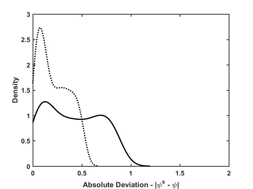
(a) Specification 1

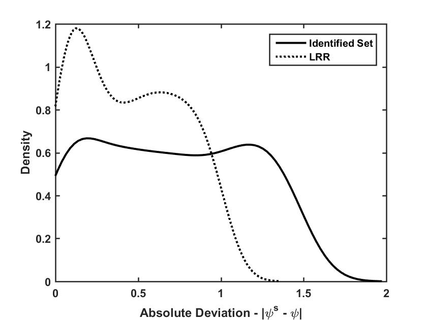
(b) Specification 2

Figure 2. Distribution of the Absolute Difference Between Predicted ATEs and the True ATE

To do so, we draw $s=1,...,1000$ values $\psi^{s}$ from the average (conservative) 95% confidence set for the LRR or the identified set described in Table 1. These sets would be the predictions reported by an empirical researcher, who does not observe or point-identify the true $\psi(\beta_{0},\gamma_{0},\pi_{0})$ due to top-coding. We draw these vectors in 2 different ways: (i) uniformly (i.e. any parameter within the appropriate set is drawn with equal probability) and (ii) furthest-case (i.e. we draw the parameters in each set that generate average predictions furthest away from the true values). To showcase the results, in Figure 2, we report the distribution of the absolute deviation $\left|\psi^{s}-\psi(\beta_{0},\gamma_{0},\pi_{0})\right|$: i.e. how do the predictions using the LRR and the identified set differ from the true value.

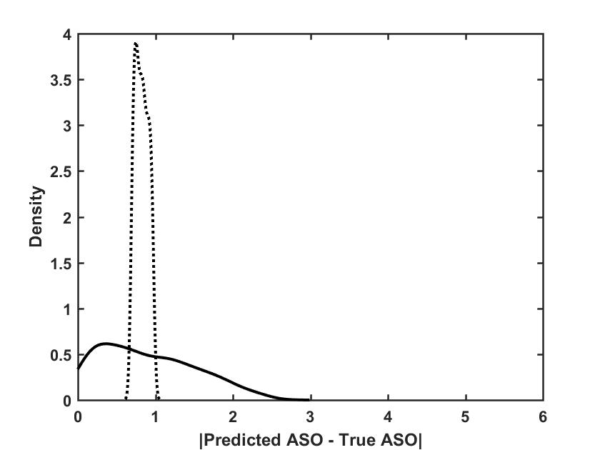
(a) Average Prediction, under $\pi^{s}=0.25$

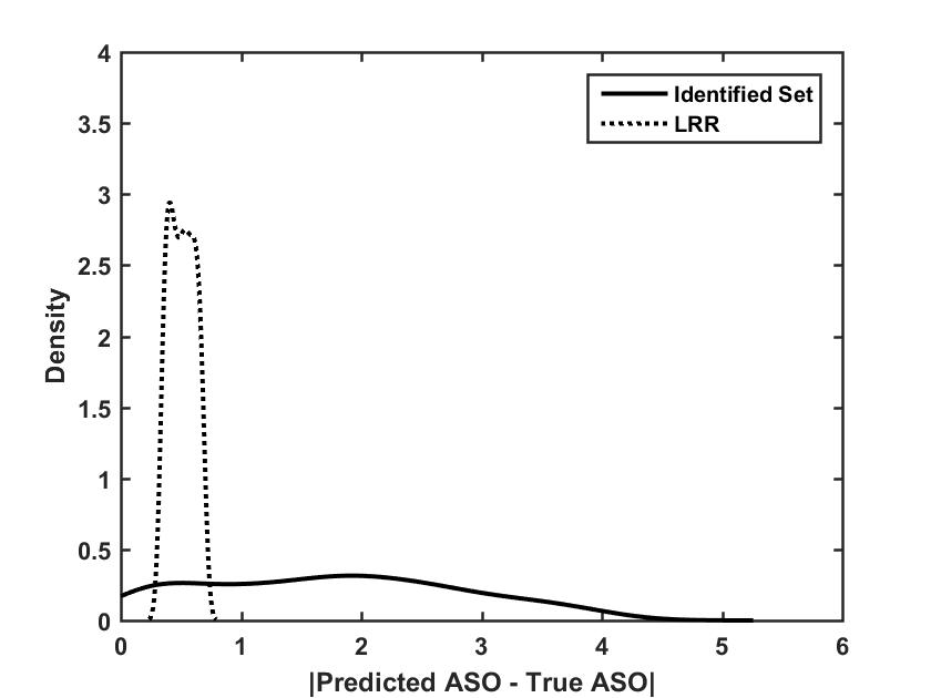
(b) Average Prediction, under $\pi^{s}=0.5$

Figure 3. Distribution of the Absolute Difference Between Predicted ASOs and the True ASO

[INSERT FIGURES 2 AND 3 HERE]

As we can see, the LRR’s predictions vary less than those with the identified set (they are often at least 30% shorter), regardless of the specification or how the parameters are drawn. The use of the LRR seems particularly favorable when (i) the identified set is large (Specification 2), and (ii) when there is a significant chance of drawing extreme values of parameters from the identified set. This difference is most salient when the furthest-care scenario is particularly important to the researcher (for instance, when a bad policy could be very costly in terms of welfare). Afterall, the LRR’s objective is not about mean predictions, but rather as minimizing the worst case.

The specifications above satisfy the LRR hypothesis, since the true $\psi(\beta_{0},\gamma_{0},\pi_{0})$ is in the LRR set. Does the LRR still preserve these favorable properties even if the LRR hypothesis is not satisfied? We investigate this question in a last exercise. We set $(\beta_{0},Z_{1},Z_{2})$ to the same values as Specification 1, but we increase $\gamma_{0}$ to 2.5. As a result, $\gamma_{0}$ is no longer in the LRR. We then compare the performance of the LRR and of the identified set in predicting the Average Structural Outcome (ASO) obtained using (2.8). This outcome is unobserved, but it can be predicted based on the LRR and the identified set. The results are shown in Figure 3. In contrast to Figure 2, some draws of the identified set can outpredict the LRR. Afterall, the former contains the true parameters which are now absent in the LRR. Nevertheless, the LRR still generates more stable predictions, and its gains are still most noticeable and relevant when the identified set is large and/or worst-case outcomes are likely. Hence, while our results rely on the simulation designs motivated by our empirical application, the approach of LRR seems to generates predictions with stable performance regardless of whether the LRR hypothesis is satisfied or not.

5. Empirical Illustration

We provide an empirical application to illustrate how our procedure works with data. The application considers the case of top-coded data, as in the Monte Carlo simulations. We focus on the returns to college education, a topic subject to a large body of work in economics (see Oreopoulos/Petronijevic:13:ERIC for a survey). For the purpose of illustration, we choose a simplified approach and focus on the ATE defined in (3.27). Depending on the question of interest, such a parameter could allow the evaluation of policies meant to increase enrollment, such as changing taxes or subsidies for college (see Dynarski/Scott:17:Tax for an overview of different policies in place in the U.S. and their associated costs). These policies could have large fiscal and welfare consequences.

In this set-up, the outcome ($Y_{i}$) is the log of the hourly wages, the policy treatment is attending college (i.e. $D_{i}\in\{0,1\}$, where $D_{i}=1$ represents that $i$ attended college and $0$ otherwise) and $X_{1,i}$ are individual covariates such as gender and/or race. Finally, the decision to attend college may depend on unobserved types: some types may have higher wages and/or benefit more from college. We model this by the random variable $\eta$, which is assumed to be binary: the returns from treatment $D_{i}=1$ may depend on whether unobserved type is high ($\eta=1$) or low ($\eta=0$) and this difference can exist throughout the distribution of $X_{1,i}$.

Since top-coding is prevalent in wage data (it is present in such widely used datasets as the NLSY and the Current Population Survey - CPS) and such top-coding is not random (for example, college educated individuals are more likely to be top-coded since they have higher wages on average), this set-up is nested within Example 3.3.2. Hence, the identified set is given in (2.6) and the LRR in (3.13) can be used with the expressions defined in and above (3.25).

We follow Romano/Shaikh:10:Eca and use data from the 2000 Annual Demographic Supplement of the Current Population Survey (CPS), keeping individuals aged 20 to 24, white, with a primary source of income from wages and salaries and that worked at least 2 hours per week on average. Akin to their work, our covariates $X_{1,i}$ are a constant and a binary variable for Male/Female. We differ from their sample by keeping both college graduates and non-college graduates, since that is our counterfactual of interest. This yields a sample of 5816 individuals, of which 826 (14%) are treated ($D_{i}=1$). Details on the data construction are provided in the Supplemental Note. We then explore the effects of different amounts of top-coding on the results.

Following the large literature on Mincerian equations (see Heckman/Humphries/Veramendi:18:JPE for a discussion), we use a linear specification for $g_{1}$:

$$g_{1}(\beta_{0}D+X_{1}^{\prime}\gamma_{0})=\beta_{0}D+X_{1}^{\prime}\gamma_{0}.$$

For the reduced form for $\eta=0$, we parametrize $g_{2}(\beta_{0}D+X_{1}^{\prime}\gamma_{0})=\log(g_{1}(\beta_{0}D+X_{1}^{\prime}\gamma_{0}))$. We present confidence sets for both the identified set for the ATE, $\psi_{0}=\psi(\beta_{0},\gamma_{0},\pi_{0})$, and the LRR for $\psi_{0}$ using both conservative and a Bonferroni-correction based inference. We present results for this data under different top-coding amounts, imposing either 5% or 10% top-coding in the sample, under a value of top possible wages of $Z_{2}=10^{8}$. The results are shown below. As standard, we report the returns to a year of college (i.e. $\psi_{0}/4$).

[INSERT TABLE 2 HERE]

Our estimates are largely consistent with the literature, including the ATE found in works as Carneiro/Heckman/Vytlacil:11:AER, despite the different sample. While the identified set is large, including ATE close to 0 and others close to 25%, the LRR is significantly shorter, between 3 and 11% (for 5% top-coding) and between 0 and 10% (for 10% top-coding). These results are also robust to different choices of $\kappa$.

To see the usefulness of the refinement in this context, consider one of the policies motivating this exercise. This could be a change in subsidies to college or expanding college loans with the purpose of a large increase in college attendance. In the presence of top-coding, the identified set cannot reject large rates of return for college (e.g. above 12% a year) - suggesting a rationale for financially costly policies. However, the LRR rejects these larger values, finding rates of return that are lower than 11% and more compatible with those observed in the literature. The LRR suggests that more costly counterfactual policies should not be undertaken. This rejection is not due to the informational content of the model, which is still captured by the identified set, but rather from the robustness of the counterfactual predictions. The larger returns to college found in the identified set seem to be driven by features of the model the researcher is less confident about.

6. Conclusion

This paper explores methods to deal with models with multiple reduced forms for counterfactual analysis. As mentioned by Eizenberg:14:ReStud, there is an inherent tradeoff within the partial identification literature: while researchers may prefer not to impose strong identifying assumptions, they must confront the issue of counterfactuals with larger identified sets when doing policy analysis.

This paper points out that not all the values of the parameter are equally desirable for counterfactual analysis despite their empirical relevance. In particular, this paper focuses on the robustness property of the parameter values when the reduced form selection rule is locally perturbed. Thus the refinement looks at the subset of counterfactual scenarios that give most reliable predictions against a range of perturbations of the reduced forms (such as through changing equilibrium selection rules).

There could be other ways to discriminate different values of the identified set depending on the purpose of the counterfactual analysis in the application. For example, one may consider local misspecification of causal relationships between certain variables. This is plausible when the researcher is not sure about the direction of causality between certain variables. Similarly as we do in this paper, one may want to find a refinement that is robust to this type of misspecification. A fruitful formulation of this approach is left for future research.

Tables and Figures

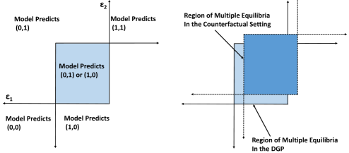
Figure 1. Locally Robust Refinement for the Entry Game Example

Notes: The figure is based on Figure 1 of Ciliberto/Tamer:09:Eca and presents a graphical analysis of the LRR for the entry game example. In the data, the region in light blue is the region of multiple equilibria which is the set $A_{3,\beta,\gamma}(X)\cap A_{4,\beta,\gamma}(X)$. In our counterfactual setting involving $X$ changed to, say, $\tilde{X}$, this region becomes $A_{3,\beta,\gamma}(\tilde{X})\cap A_{4,\beta,\gamma}(\tilde{X})$ depicted in dark blue in the right hand side figure. The LRR chooses nuisance parameters in their identified set that minimize the probability mass in the dark blue region.

Notes: The figure presents the absolute deviation of the predicted statistic, $\psi^{s}$ drawn from the 95% confidence set for the LRR or Identified set from the specifications in Section 4.2, relative to the parameter of interest, $\psi(\beta_{0},\gamma_{0},\pi_{0})$, used for policy analysis. We present the uniformly-drawn parameters case, where we draw $\psi^{s}$ with equal probability from their respective sets $S=1000$ times. Drawing the furthest away parameter from the true values always yield the same parameter draw (so it is not pictured above). In the latter case, the mean absolute deviation is 0.521 for the LRR and 0.895 for the identified set for Specification 1, and 1.012 and 1.492 respectively for Specification 2.

Notes: The figure presents the absolute deviation of the predicted ASO, $\text{ASO}^{s}=\mathbf{E}\pi^{s}(\gamma^{s}+\beta^{s}D)+(1-\pi^{s})\log(\gamma^{s}+\beta^{s}D)$, to the ASO under the true parameters $(\beta_{0},\pi_{0},\gamma_{0})=(0.15,0.5,2.5)$ across draws $s=1,...,1000$. For the predicted outcome, we set $\pi^{s}$ at either 0.25 or 0.5 (true value), and draw the remaining parameters $S=1000$ times from the LRR or the identified set (calculated numerically).

Table 1. The Empirical Coverage Probability and Average Length of Confidence Intervals for $\psi(\beta_{0},\gamma_{0},\pi_{0})$ at 95% Nominal Level.

Coverage Probability

		Specification 1		Specification 2
$\psi$		Least Favorable	RSW	Least Favorable	RSW
Identified Set	$n=500$	1	0.996	1	1
LRR	$n=500$	0.95	0.95	1	1

Average Length of CI

		Specification 1		Specification 2
$\psi$		Least Favorable	RSW	Least Favorable	RSW
Identified Set	$n=500$	1.040	0.923	1.637	1.477
LRR	$n=500$	0.666	0.666	1.157	1.157

Notes: The first half of the table reports the empirical coverage probability of the confidence interval for $\psi$ computed with the bootstrap procedure described in the main text, and the second half reports its average length for the specifications described in the main text. The first inference procedure, denoted “LF”, follows the conservative approach defined in the main text, while the second is denoted “RSW” and uses the Bonferroni-based modification of Romano/Shaikh/Wolf:14:Eca.

Table 2. Confidence Intervals for $\psi$ (ATE), Parameter of Interest

	5% top-coding	10% top-coding
Identified Set - LF	[0.023, 0.245]	[0, 0.245]
Identified Set - RSW	[0.041, 0.245]	[0, 0.245]
LRR - LF	[0.034, 0.110]	[0, 0.091]
LRR - RSW	[0.041, 0.110]	[0, 0.091]

Notes: The Table presents the results for the empirical application described in the main text, where we use the data and top-code it at different values (5% or 10%), assuming the top wage is $Z_{2}=10^{8}$. The first inference procedure, denoted “LF”, follows the conservative approach defined in the main text - see equation (4.10), while the second is denoted “RSW” and uses the Bonferroni-based modification of Romano/Shaikh/Wolf:14:Eca, see equation (4.16).

7. Appendix: Mathematical Proofs

7.1. Proof of Theorem 3.1

Proof of Theorem 3.1: Let $U$ and $\mathcal{W}$ be the sets from which $\eta$ and $W=(X,\varepsilon)$ take values respectively. Let $\mathcal{H}$ be the collection of measurable maps $h:\mathcal{W}\times U\rightarrow\mathbf{R}$ such that

$$\int h(w,\eta)d\mu(\eta)=0,\tilde{F}\text{-a.s.,}\text{ and }\int\int h^{2}(w,\eta)d\mu(\eta)d\tilde{F}(w)<\infty.$$ (7.1)

We endow $\mathcal{H}$ with the inner-product $\langle\cdot,\cdot\rangle$ as follows: for $h_{1},h_{2}\in\mathcal{H}$,

$$\langle h_{1},h_{2}\rangle=\int\int h_{1}(w,\eta)h_{2}(w,\eta)d\mu(\eta)d\tilde{F}(w).$$ (7.2)

Then $(\mathcal{H},\langle\cdot,\cdot\rangle)$ is a Hilbert space (up to an equivalence class). Recall that all distributions $G\in\mathcal{G}$ are dominated by the uniform distribution $\mu$ over $H$. Define $\|h\|^{2}=\langle h,h\rangle$ and write

$$\delta_{\mathcal{G}}(G^{\prime},G)=\left\|\frac{dG^{\prime}}{d\mu}-\frac{dG}{d\mu}\right\|,$$ (7.3)

and $\textsf{ASO}_{\beta,\gamma}(G)=\int\int\rho_{\beta,\gamma}(w;\eta)dG(\eta|w)d\tilde{F}(w)$. If we define

$$\Delta_{\beta,\gamma}(\eta,w)=\rho_{\beta,\gamma}(w;\eta)-\int\rho_{\beta,\gamma}(w;\eta)d\mu(\eta),$$ (7.4)

we can write

$$\sup_{G^{\prime}\in\mathcal{G}:\delta_{\mathcal{G}}(G^{\prime},G)\leq K}\frac{|\textsf{ASO}_{\beta,\gamma}(G^{\prime})-\textsf{ASO}_{\beta,\gamma}(G)|}{\delta_{\mathcal{G}}(G^{\prime},G)}=\sup_{h^{\prime}\in\mathcal{H}:\|h^{\prime}\|=K}\frac{\left\langle\rho_{\beta,\gamma},h^{\prime}\right\rangle}{\|h^{\prime}\|}=\sup_{h^{\prime}\in\mathcal{H}:\|h^{\prime}\|=K}\frac{\left\langle\Delta_{\beta,\gamma},h^{\prime}\right\rangle}{\|h^{\prime}\|},$$

where the first equality comes because $dG^{\prime}/d\mu-dG/d\mu\in\mathcal{H}$ (from the fact that each density integrates to one) and the second equality comes from the fact that for all $h\in\mathcal{H}$, $\int h(w,\eta)d\mu(\eta)=0$. Since $\Delta_{\beta,\gamma}\in\mathcal{H}$ by Assumption 3.1, using (7.1) and Cauchy-Schwarz inequality, we can achieve the last supremum by taking $h^{\prime}$ in the supremum to be $K\Delta_{\beta,\gamma}/\|\Delta_{\beta,\gamma}\|$. The result is nothing but $\sqrt{Q^{\mathsf{LRR}}(\beta,\gamma)}$, completing the proof. $\blacksquare$

Supplemental Note to “Counterfactual Analysis under Partial Identification Using Locally Robust Refinement”

Nathan Canen and Kyungchul Song

University of Houston and University of British Columbia

This note consists of three parts. In the first part (Appendix A), we present the proof of the uniform asymptotic validity of our inference, beginning with various auxiliary results. In the second part (Appendix B), we provide further details on the data used for the empirical application in Section 5. In Appendix C, we provide a notation table as a convenient reference.

Appendix A Uniform Asymptotic Validity of the Confidence Region Under the LRR Hypothesis

A.1. Uniform Asymptotic Validity

This section establish the uniform validity of the inference on LRR. To make explicit their dependence on $P$, we write $\tilde{F}$, $Q^{\mathsf{LRR}}(\beta,\gamma)$, and $\Gamma_{\kappa}^{\mathsf{LRR}}$ as $\tilde{F}_{P}$, $Q_{P}^{\mathsf{LRR}}(\beta,\gamma)$, and $\Gamma_{\kappa,P}^{\mathsf{LRR}}$ in this section. We first, make the following assumption.

Assumption A.1.

For each $\varepsilon>0$,

$$\limsup_{n\rightarrow\infty}\sup_{P\in\mathbf{P}}P\left\{\sup_{(\beta,\gamma)\in\Theta}\left|\hat{Q}^{\mathsf{LRR}}(\beta,\gamma)-Q_{P}^{\mathsf{LRR}}(\beta,\gamma)\right|>\varepsilon\right\}=0.$$ (A.1)

Assumption A.1 requires uniform consistency of the sample criterion function for the LRR (uniform in $(\beta,\gamma)\in\Theta$ and $P\in\mathbf{P}$). Typically, $Q_{P}^{\mathsf{LRR}}(\beta,\gamma)$ takes the following form:

$$Q_{P}^{\mathsf{LRR}}(\beta,\gamma)=\int q(x;\beta,\gamma)d\tilde{F}_{P}(x),$$

for some map $q$ and a distribution $\tilde{F}_{P}$. Let $\hat{F}(x)$ and $\hat{q}(x;\beta,\gamma)$ be the estimated versions of $\tilde{F}_{P}(x)$ and $q(x;\beta,\gamma)$ using which we construct

$$\hat{Q}^{\mathsf{LRR}}(\beta,\gamma)=\int\hat{q}(x;\beta,\gamma)d\hat{F}(x).$$

(Note that when the researcher knows fully $\tilde{F}_{P}$ under the counterfactual scenario of focus, she can simply take $\hat{F}$ to be $\tilde{F}_{P}$.) Thus, we can find lower level conditions for (A.1) in terms of $\hat{F}(x)$ and $\hat{q}(x;\beta,\gamma)$ using standard arguments.

We let

$$m_{j,P}(\beta,\gamma)=\mathbf{E}_{P}[m_{j}(Z_{i};\beta,\gamma)],\text{ and }\sigma_{j,P}^{2}(\beta,\gamma)=\text{Var}_{P}(m_{j}(Z_{i};\beta,\gamma)),$$ (A.2)

where $\text{Var}_{P}$ denotes the variance under $P$. Let

$$\mu_{i,j,P}(\beta,\gamma)=\frac{m_{j}(Z_{i};\beta,\gamma)}{\sigma_{j,P}(\beta,\gamma)}.$$ (A.3)

Let us make the following assumption.

Assumption A.2.

(i) There exist $C>0$ and $q\geq 2$ such that

$$\max_{1\leq j\leq k}\sup_{P\in\mathbf{P}}\mathbf{E}_{P}\left[\sup_{(\beta,\gamma)\in\Theta}\left|\mu_{i,j,P}(\beta,\gamma)\right|^{q+1}\right]<C.$$ (A.4)

(ii) There exists $C>0$ such that for any $\delta>0$ and any $\theta=(\beta,\gamma)\in\Theta$,

$$\max_{1\leq j\leq k}\sup_{P\in\mathbf{P}}\mathbf{E}_{P}\left[\sup_{\theta^{\prime}\in\Theta:\|\theta-\theta^{\prime}\|\leq\delta}\left|\mu_{i,j,P}(\theta)-\mu_{i,j,P}(\theta^{\prime})\right|^{2}\right]<C\delta^{2}.$$ (A.5)

(iii) $\Theta$ is compact.

Assumption A.2(i) is a uniform moment condition. Assumption A.2(ii) imposes the condition of $L_{2}$-equicontinuity on the function $\mu_{i,j,P}(\beta,\gamma)$. This condition, similar in spirit to Chen/Linton/vanKeilegom:71:Eca, is used to verify the asymptotic equicontinuity of the empirical process involved in $\hat{Q}(\beta,\gamma)$ and its bootstrap version.

We now introduce an assumption on the limit Gaussian process of the empirical process. First, let us introduce some notation. Let $\{\nu_{j,P}(\beta,\gamma):(\beta,\gamma)\in\Theta\}$ be a Gaussian process having covariance function equal to $\text{Cov}_{P}(\mu_{i,j,P}(\beta,\gamma),\mu_{i,j,P}(\bar{\beta},\bar{\gamma}))$, $(\beta,\gamma),(\bar{\beta},\bar{\gamma})\in\Theta$. Let for $M>0$,

$$\zeta_{M,P}^{\mathsf{sum}}(\beta,\gamma;r) =\sum_{j=1}^{p}\min\left\{[\nu_{j,P}+r_{j}]_{+}(\beta,\gamma),M\right\},\text{ and }$$ (A.6)

$$\zeta_{P}^{\mathsf{min}}(\beta,\gamma) =\min_{1\leq j\leq p}\nu_{j,P}(\beta,\gamma),$$ (A.7)

where $r=(r_{j})_{j=1}^{p}$ is a vector of real measurable maps on $\Theta$. Define

$$R_{M}=\{(r_{j})_{j=1}^{p}:r_{j}\text{ is measurable, and }-M\leq r_{j}(\cdot)\leq 0,\text{ for all }j=1,...,p\}.$$ (A.8)

Assumption A.3.

There exists $M_{0}>0$ such that the conditions below hold for $\zeta_{M,P}(\beta,\gamma;r)=\zeta_{M,P}^{\mathsf{sum}}(\beta,\gamma;r)$ or $\zeta_{M,P}(\beta,\gamma;r)=-\zeta_{P}^{\mathsf{min}}(\beta,\gamma)$.

(i) For any $M>M_{0}$ and any $0<c<pM$,

$$\sup_{P\in\mathbf{P}}\sup_{r\in R_{M}}\sup_{(\beta,\gamma)\in\Theta_{P}}P\{c-\varepsilon\leq\zeta_{M,P}(\beta,\gamma;r)\leq c+\varepsilon\}\rightarrow 0,$$ (A.9)

as $\varepsilon\rightarrow 0$.

(ii) For any $M>M_{0}$, there exists $\varepsilon_{M}>0$ such that for any $0<c<pM$, the slope of the CDF of $\zeta_{M,P}(\beta,\gamma;r)$ at $c$ is bounded from below by $\varepsilon_{M}$ for all $(\beta,\gamma)\in\Theta_{P},r\in R_{M}$, and $P\in\mathbf{P}$.

Assumption A.3(i) is a mild regularity condition for the Gaussian process $\nu_{P}$, which is generically satisfied because the Gaussian process has an unbounded support. (Note that $R_{M}$ is a collection of vectors of functions that are bounded between $-M$ and $0$.) The assumption can be violated when $\nu_{j,P}(\beta,\gamma)$ has zero variance at some point $(\beta,\gamma)\in\Theta_{P}$. Assumption A.3(ii) is a technical condition which requires that $\zeta_{M,P}(\beta,\gamma;r)$ has CDF strictly increasing at any $c\in(0,pM)$ with slope bounded away from zero uniformly over $(\beta,\gamma)\in\Theta_{P},r\in R_{M}$, and $P\in\mathbf{P}$. Note that when the Gaussian process $\nu_{P}$ has an unbounded support for all $(\beta,\gamma)\in\Theta_{P}$ and $P\in\mathbf{P}$, the support of $\zeta_{M,P}(\beta,\gamma;r)$ is $[0,pM]$ for all $(\beta,\gamma)\in\Theta_{P},r\in R_{M}$, and $P\in\mathbf{P}$. Thus Assumption A.3(ii) is not implausible.

The following theorem gives the uniform asymptotic validity of the confidence region $\tilde{C}_{1-\alpha}^{\mathsf{LRR}}$ defined in (4.16).

Theorem A.1.

Suppose that Assumptions A.1 and A.2 hold. Then,

$$\liminf_{n\rightarrow\infty}\inf_{P\in\mathbf{P}}\inf_{(\beta,\gamma)\in\Theta_{P}}P\left\{(\beta,\gamma)\in\tilde{C}_{1-\alpha}^{\mathsf{LRR}}\right\}\geq 1-\alpha.$$ (A.10)

For the proof of uniform asymptotic validity, we approximate the bootstrap distribution by a truncated version of a functional of a Gaussian process. This facilitates the use of the continuous mapping theorem in Linton/Song/Whang:10:JOE which does not require that the continuous functionals have a well defined limit.

The rest of Appendix A is devoted to proving Theorem A.1.

A.2. Auxiliary Results I: General Results on Empirical Processes

We introduce a theorem that gives the weak convergence of a stochastic process to a tight limit along a given sequence of probabilities. This result is based on Section 2.8.3 of vanderVaart/Wellner:96:WeakConvg. We modify the results slightly because in our case the class of functions that index an empirical process depends on the underlying distribution $P\in\mathbf{P}$. The notation in this subsection is self-contained.

Let $\mathcal{T}$ be a given set and let $f_{j,P}(\cdot;\tau):\mathbf{R}^{d}\rightarrow\mathbf{R}$, $j=1,...,k$, be a function indexed by $\tau\in\mathcal{T}$, potentially depending on $P\in\mathbf{P}$. Define for each $j=1,...,k$,

$$\mathscr{F}_{j,P}=\{f_{j,P}(\cdot;\tau):\tau\in\mathcal{T}\},\text{ and }\mathscr{F}_{P}=\{f_{P}(\cdot;\tau):\tau\in\mathcal{T}\},$$ (A.11)

where $f_{P}(\cdot;\tau)=[f_{1,P}(\cdot;\tau),...,f_{k,P}(\cdot;\tau)]^{\prime}$. Given i.i.d. random vectors $X_{i}$, we introduce a stochastic process on $\mathcal{T}$:

$$\nu_{n,P}(\tau)=\frac{1}{\sqrt{n}}\sum_{i=1}^{n}(f_{P}(X_{i};\tau)-\mathbf{E}_{P}[f_{P}(X_{i};\tau)]).$$

We let $\ell^{\infty}(\mathcal{T})$ be the set of bounded $\mathbf{R}^{k}$-valued functions on $\mathcal{T}$, and $\|\cdot\|_{\infty}$ denote the sup norm on $\ell^{\infty}(\mathcal{T})$, i.e., $\|\nu\|_{\infty}=\sup_{\tau\in\mathcal{T}}\|\nu(\tau)\|$, $\nu\in\ell^{\infty}(\mathcal{T})$, where $\|\cdot\|$ denotes the Euclidean norm in $\mathbf{R}^{k}$. We introduce a semimetric $\rho_{P}$ on $\mathcal{T}$ as follows:

$$\rho_{P}(\tau_{1},\tau_{2})=\sqrt{\mathbf{E}_{P}\left[\|f_{P}(X_{i};\tau_{1})-f_{P}(X_{i};\tau_{2})\|^{2}\right]}.$$

Define the class of bounded Lipschitz functionals:

$$\quad\quad\text{BL}_{1}=\left\{\rho:\ell^{\infty}(\mathcal{T})\rightarrow\mathbf{R}:|\rho(\nu_{1})-\rho(\nu_{2})|\leq\|\nu_{1}-\nu_{2}\|_{\infty},\sup_{\nu\in\ell^{\infty}(\mathcal{T})}|\rho(\nu)|\leq 1\right\}.$$ (A.12)

Write the $L_{2}(P)$ norm by $\|f\|_{P,2}=\sqrt{\mathbf{E}_{P}\|f(X_{i})\|^{2}}.$ Given a class $\mathscr{F}_{P}$ of $\mathbf{R}^{k}$-valued measurable functions, let $N_{[]}(\varepsilon,\mathscr{F}_{P},\|\cdot\|_{P,2})$ be the $\varepsilon$-bracketing entropy of $\mathscr{F}_{P}$ with respect to the $L_{2}(P)$ norm, which is the smallest number $N$ of the brackets $\{[\ell_{j},u_{j}]\}_{j=1}^{N}$ such that each $f\in\mathscr{F}_{P}$ satisfies $\ell_{j}\leq f\leq u_{j}$ for some $[\ell_{j},u_{j}]$ and $\|\ell_{j}-u_{j}\|_{P,2}\leq\varepsilon$. (The inequalities required of the brackets are point-wise inequalities when $f$ is $\mathbf{R}^{k}$-valued.)

We also define $P^{*}$ and $\mathbf{E}_{P}^{*}$ to be the outer-probability and the outer-expectation under $P$. (See vanderVaart/Wellner:96:WeakConvg, Section 1.2 for details.) The following theorem formulates conditions for the weak convergence of $\nu_{n,P}$ to a tight Gaussian limit uniformly over $P\in\mathbf{P}$.

Theorem A.2.

Suppose that the two conditions are satisfied.

(i) For each $j=1,...,k$, there exists a measurable envelope $F_{j,P}$ for $\mathscr{F}_{j,P}$ such that

$$\sup_{P\in\mathbf{P}}\mathbf{E}_{P}[F_{j,P}^{2}(X_{i})]<\infty.$$ (A.13)

(ii)

$$\int_{0}^{\infty}\sup_{P\in\mathbf{P}}\sqrt{\log N_{[]}(\varepsilon\|F_{j,P}\|_{P,2},\mathscr{F}_{j,P},\|\cdot\|_{P,2})}d\varepsilon<\infty.$$ (A.14)

Then, we have

$$\sup_{f\in\text{BL}_{1}}\sup_{P\in\mathbf{P}}\left|\mathbf{E}_{P}^{*}[f(\nu_{n,P})]-\mathbf{E}_{P}[f(\nu_{P})]\right|\rightarrow 0,\text{ as }n\rightarrow\infty,$$ (A.15)

and

$$\lim_{\delta\downarrow 0}\sup_{P\in\mathbf{P}}\mathbf{E}_{P}\left[\sup_{\rho_{P}(\tau_{1},\tau_{2})<\delta}\|\nu_{P}(\tau_{1})-\nu_{P}(\tau_{2})\|\right]=0,$$ (A.16)

where $\nu_{P}=[\nu_{1,P},...,\nu_{p,P}]^{\prime}$ is an $\mathbf{R}^{p}$-valued Gaussian process with covariance kernel given by

$$\mathbf{E}[\nu_{j,P}(\tau_{1})\nu_{\ell,P}(\tau_{2})]=\text{Cov}_{P}\left(f_{j,P}(X_{i};\tau_{1}),f_{\ell,P}(X_{i};\tau_{2})\right),\tau_{1},\tau_{2}\in\mathcal{T},$$

for $j,\ell=1,...,p$.

Proof: By following the proof of Theorem 2.8.4 of vanderVaart/Wellner:96:WeakConvg, we find that Conditions (i) and (ii) give the asymptotic equicontinuity of the following form: for every $\varepsilon>0$,

$$\lim_{\delta\downarrow 0}\limsup_{n\rightarrow\infty}\sup_{P\in\mathbf{P}}P^{*}\left\{\sup_{\rho_{P}(\tau_{1},\tau_{2})<\delta}\left\|\nu_{n,P}(\tau_{1})-\nu_{n,P}(\tau_{2})\right\|>\varepsilon\right\}=0,$$ (A.17)

and $(\mathcal{T},\rho_{P})$ is totally bounded uniformly over $P\in\mathbf{P}$ in the sense that for any $\varepsilon>0$, and any $P\in\mathbf{P}$ there exists an $m_{\varepsilon}$ number of $\varepsilon$-open balls (with respect to $\rho_{P}$) that cover $\mathcal{T}$ where $m_{\varepsilon}$ does not depend on $P$. Then both the results of (A.15) and (A.16) follow by Theorem 2.6 of Gine/Zinn:91:AP. $\blacksquare$

We consider a bootstrap version of Theorem A.2. Given a sample $\{X_{1},...,X_{n}\}$, we let $\mathscr{G}_{n}$ be the $\sigma$-field generated by this sample. Let $\hat{P}$ be the empirical measure of $\{X_{1},...,X_{n}\}$, and $\{X_{1}^{*},...,X_{n}^{*}\}$ i.i.d. draws from $\hat{P}$. First, define

$$\nu_{n,P}^{*}(\tau)=\frac{1}{\sqrt{n}}\sum_{i=1}^{n}(f_{P}(X_{i}^{*};\tau)-\mathbf{E}_{\hat{P}}[f_{P}(X_{i}^{*};\tau)]),$$

which is the bootstrap counterpart of $\nu_{n,P}$.

Theorem A.3.

Suppose that the conditions of Theorem A.2 are satisfied. Then for any $\varepsilon>0$,

$$\sup_{P\in\mathbf{P}}P\left\{\sup_{f\in\text{BL}_{1}}\left|\mathbf{E}[f(\nu_{n,P}^{*})|\mathscr{G}_{n}]-\mathbf{E}_{P}[f(\nu_{P})]\right|>\varepsilon\right\}\rightarrow 0,$$ (A.18)

as $n\rightarrow\infty$, where $\nu_{P}$ is the Gaussian process in Theorem A.2.

Proof: The proof basically follows that of Lemma A.2 of Linton/Song/Whang:10:JOE. The only difference here is that the class $\mathcal{F}_{P}$ depends on $P$. As seen in the proof of Theorem A.2, $(\mathcal{T},\rho_{P})$ is totally bounded uniformly over $P\in\mathbf{P}$. Then $(\mathcal{T}-\mathcal{T},\rho_{P})$ is totally bounded uniformly over $P\in\mathbf{P}$ as well, where $\mathcal{T}-\mathcal{T}=\{\tau_{1}-\tau_{2}:\tau_{1},\tau_{2}\in\mathcal{T}\}$. For any given $\varepsilon>0$, there is a map $\pi_{\varepsilon}:\mathcal{T}\rightarrow\mathcal{T}$ which takes $m_{\varepsilon}$ values and $\rho_{P}(\pi_{\varepsilon}\tau,\tau)\leq\varepsilon$. Take any $f\in\text{BL}_{1}$, and consider

$$\left|\mathbf{E}[f(\nu_{n,P}^{*})|\mathscr{G}_{n}]-\mathbf{E}_{P}f(\nu_{P})\right| \leq\left|\mathbf{E}[f(\nu_{n,P}^{*})|\mathscr{G}_{n}]-\mathbf{E}[f(\nu_{n,P}^{*}\circ\pi_{\varepsilon})|\mathscr{G}_{n}]\right|$$ (A.19)

$$\quad+\left|\mathbf{E}[f(\nu_{n,P}^{*}\circ\pi_{\varepsilon})|\mathscr{G}_{n}]-\mathbf{E}_{P}f(\nu_{P}\circ\pi_{\varepsilon})\right|$$

$$\quad+\left|\mathbf{E}_{P}f(\nu_{P}\circ\pi_{\varepsilon})-\mathbf{E}_{P}f(\nu_{P})\right|.$$

The last term vanishes uniformly in $f\in\text{BL}_{1}$ as $\varepsilon\rightarrow 0$ by (A.16). By using the proof of Lemma 2.1 in Gine/Zinn:91:AP, p.763, and the moment condition (A.13) to handle the remainder part of the process that is left over from truncation, we can show that the second term on the right hand side vanishes in probability uniformly over $P\in\mathbf{P}$ as $n\rightarrow\infty$. We deal with the first term using Le Cam’s Poissonization lemma and following the proof of Theorem 2.2 of Gine:97:LectureNotes, p.104. More specifically, we define $\mathcal{T}(\varepsilon,\rho_{P})=\{\tau_{1}-\tau_{2}\in\mathcal{T}-\mathcal{T}:\rho_{P}(\tau_{1},\tau_{2})<\varepsilon\}$, and note that

$$\mathbf{E}_{P}\left[\mathbf{E}\left[\sup_{\tau\in\mathcal{T}(\varepsilon,\rho_{P})}\|\nu_{n,P}^{*}(\tau)\||\mathscr{G}_{n}\right]\right]$$ (A.20)

$$\leq\frac{e}{e-1}\left\{\mathbf{E}_{P}\left[\sup_{\tau\in\mathcal{T}(\varepsilon,\rho_{P})}\left\|\frac{1}{\sqrt{n}}\sum_{i=1}^{n}(N_{i}-1)(f_{P}(X_{i};\tau)-\mathbf{E}_{P}[f_{P}(X_{i};\tau)])\right\|\right]\right\}$$

$$\quad+\mathbf{E}_{P}\left[\left|\frac{1}{\sqrt{n}}\sum_{i=1}^{n}(N_{i}-1)\right|\sup_{\tau\in\mathcal{T}(\varepsilon,\rho_{P})}\left\|\frac{1}{n}\sum_{i=1}^{n}f_{P}(X_{i};\tau)\right\|\right],$$

where $N_{i}$ is i.i.d. Poisson random variables with mean $1$ independent of all the other random variables. We apply Theorem A.2 to the class $\mathcal{T}(\varepsilon,\rho_{P})$, and find that both terms on the right hand, after taking supremum over $P\in\mathbf{P}$, vanish as $n\rightarrow\infty$ and $\varepsilon\rightarrow 0$. $\blacksquare$

The following lemma is the bootstrap version of Lemma A.1 of Linton/Song/Whang:10:JOE. The proof of the lemma can be proceeded similarly as in the proof of Lemma A.1 of Linton/Song/Whang:10:JOE using (A.18) and is omitted.

Lemma A.1.

Suppose that the bootstrap empirical process $\nu_{n,P}^{*}$ satisfies (A.18) for any $\varepsilon>0$. Let $f_{n,P}$ be a continuous functional on $\ell^{\infty}(\mathcal{T})$ that is potentially $\mathscr{G}_{n}$-measurable such that for some possibly $\mathscr{G}_{n}$-measurable real-valued map $C_{n,P}$,

$$|f_{n,P}(\nu_{1})-f_{n,P}(\nu_{2})|\leq C_{n,P}\sup_{\tau\in\mathcal{T}}\left|\nu_{1}(\tau)-\nu_{2}(\tau)\right|,$$ (A.21)

for any $\nu_{1},\nu_{2}\in\ell_{\infty}(\mathcal{T})$, and for each $c\in A$ for some set $A\subset\mathbf{R}$,

$$\lim_{\varepsilon\rightarrow 0}\limsup_{n\rightarrow\infty}\sup_{P\in\mathbf{P}}P\left\{|f_{n,P}(\nu_{P})-c|\leq C_{n,P}\varepsilon\right\}=0.$$ (A.22)

Then, for each $c\in A$ and each $\varepsilon>0$,

$$\limsup_{n\rightarrow\infty}\sup_{P\in\mathbf{P}}P\left\{\left|P\left\{f_{n,P}(\nu_{n,P}^{*})\leq c|\mathscr{G}_{n}\right\}-P\{f_{n,P}(\nu_{P})\leq c\}\right|>\varepsilon\right\}=0.$$ (A.23)

A.3. Auxiliary Results II: Convergence of Stochastic Processes in Test Statistics

We apply the general results on the empirical processes in the previous section to the convergence of stochastic processes in test statistics in this paper. For this subsection, we assume that Assumptions A.1-A.3 hold.

For $j=1,...,p$, let

$$\hat{\nu}_{n,j,P}(\beta,\gamma) =\frac{\sqrt{n}(\overline{m}_{j}(\beta,\gamma)-m_{j,P}(\beta,\gamma))}{\hat{\sigma}_{j}(\beta,\gamma)},\text{ and }$$ (A.24)

$$\tilde{\nu}_{n,j,P}(\beta,\gamma) =\frac{\sqrt{n}(\overline{m}_{j}(\beta,\gamma)-m_{j,P}(\beta,\gamma))}{\sigma_{j,P}(\beta,\gamma)},$$

and let $\hat{\nu}_{n,P}=[\hat{\nu}_{n,1,P},...,\hat{\nu}_{n,p,P}]^{\prime}$, and $\tilde{\nu}_{n,P}=[\tilde{\nu}_{n,1,P},...,\tilde{\nu}_{n,p,P}]^{\prime}$. Similarly, we also take for $j=1,...,p$,

$$\hat{\nu}_{n,j}^{*}(\beta,\gamma) =\frac{\sqrt{n}(\overline{m}_{j}^{*}(\beta,\gamma)-\overline{m}_{j}(\beta,\gamma))}{\hat{\sigma}_{j}(\beta,\gamma)},\text{ and }$$ (A.25)

$$\tilde{\nu}_{n,j}^{*}(\beta,\gamma) =\frac{\sqrt{n}(\overline{m}_{j}^{*}(\beta,\gamma)-\overline{m}_{j}(\beta,\gamma))}{\sigma_{j,P}(\beta,\gamma)},$$

and let $\hat{\nu}_{n}^{*}=[\hat{\nu}_{n,1}^{*},...,\hat{\nu}_{n,p}^{*}]^{\prime}$ and $\tilde{\nu}_{n}^{*}=[\tilde{\nu}_{n,1}^{*},...,\tilde{\nu}_{n,p}^{*}]^{\prime}$. Let us first present the weak convergence results of the processes, $\tilde{\nu}_{n,j,P}(\beta,\gamma)$ and $\tilde{\nu}_{n,j}^{*}(\beta,\gamma)$. Let $\mathscr{G}_{n}$ be the $\sigma$-field generated by $\{Z_{i}\}_{i=1}^{n}$. Let $BL_{1}$ be the same as $BL_{1}$ in (A.12) except that $\mathcal{T}$ is replaced by $\Theta$.

Lemma A.2.

There exists a tight Borel measurable Gaussian process $\nu_{P}$ on $\Theta$ such that

$$\sup_{f\in\text{BL}_{1}}\sup_{P\in\mathbf{P}}\left|\mathbf{E}_{P}^{*}[f(\tilde{\nu}_{n,P})]-\mathbf{E}_{P}[f(\nu_{P})]\right|\rightarrow 0,\text{ as }n\rightarrow\infty,$$ (A.26)

and for each $\varepsilon>0$,

$$\sup_{P\in\mathbf{P}}P\left\{\sup_{f\in\text{BL}_{1}}\left|\mathbf{E}[f(\tilde{\nu}_{n}^{*})|\mathscr{G}_{n}]-\mathbf{E}_{P}[f(\nu_{P})]\right|>\varepsilon\right\}\rightarrow 0,\text{ as }n\rightarrow\infty.$$ (A.27)

Proof: For the first statement, we use Theorem A.2, and verify the conditions there. To map the current set-up to that of Theorem A.2, we take $\mathcal{T}=\Theta$ and identify $\tau=(\beta,\gamma)\in\Theta$, $X_{i}=Z_{i}$, and $f_{j,P}(Z_{i},\tau)=m_{j}(Z_{i};\beta,\gamma)/\sigma_{j,P}(\beta,\gamma)$. Condition (i) of the theorem follows by Assumption A.2(i), and Condition (ii) by Assumption A.2(ii) and the assumption that $\Theta$ is compact. Thus (A.26) follows by Theorem A.2. By Theorem A.3, the second statement follows similarly. $\blacksquare$

Lemma A.3.

For all $\varepsilon>0$,

$$\max_{1\leq j\leq p}\sup_{P\in\mathbf{P}}P\left\{\sup_{(\beta,\gamma)\in\Theta}\left|\frac{\sigma_{j,P}(\beta,\gamma)}{\hat{\sigma}_{j}(\beta,\gamma)}-1\right|>\varepsilon\right\}\rightarrow 0,$$

as $n\rightarrow\infty$.

Proof: We can show this using Assumption A.2(i) and (ii) and following the same steps in the proof of Lemma D.2 of Bugni/Canay/Shi:15:JOE. Details are omitted. $\blacksquare$

Now combining Lemmas A.2 and A.3, we obtain the following result as a corollary.

Lemma A.4.

There exists a tight Borel measurable Gaussian process $\nu_{P}$ on $\Theta$ such that

$$\sup_{f\in\text{BL}_{1}}\sup_{P\in\mathbf{P}}\left|\mathbf{E}_{P}^{*}[f(\hat{\nu}_{n,P})]-\mathbf{E}_{P}[f(\nu_{P})]\right|\rightarrow 0,\text{ as }n\rightarrow\infty,$$ (A.28)

and for each $\varepsilon>0$,

$$\sup_{P\in\mathbf{P}}P\left\{\sup_{f\in\text{BL}_{1}}\left|\mathbf{E}[f(\hat{\nu}_{n}^{*})|\mathscr{G}_{n}]-\mathbf{E}_{P}[f(\nu_{P})]\right|>\varepsilon\right\}\rightarrow 0,\text{ as }n\rightarrow\infty.$$ (A.29)

Proof: Note that

$$\hat{\nu}_{n,P}(\beta,\gamma)=\tilde{\nu}_{n,P}(\beta,\gamma)+\tilde{\nu}_{n,P}(\beta,\gamma)\left(\frac{\sigma_{j,P}(\beta,\gamma)}{\hat{\sigma}_{j}(\beta,\gamma)}-1\right).$$

By Lemma A.2, the process $\tilde{\nu}_{n,P}$ is asymptotically uniformly tight uniformly over $P\in\mathbf{P}$. By Lemma A.3, the last term on the right hand side is $o_{P}(1)$ uniformly over $(\beta,\gamma)\in\Theta$ and over $P\in\mathbf{P}$. Lemma A.2 then yields the first result of the lemma. The proof for the second result is similar. $\blacksquare$

Lemma A.5.

$$\inf_{P\in\mathbf{P}}P\left\{\Gamma_{\kappa,P}^{\mathsf{LRR}}(\beta)\subset\hat{\Gamma}_{\kappa}^{\mathsf{LRR}}(\beta),\forall\beta\in B\right\}\rightarrow 1,$$ (A.30)

as $n\rightarrow\infty$.

Proof: In light of Assumption A.1, it suffices to show that for all $\varepsilon>0$,

$$\sup_{P\in\mathbf{P}}P\left\{\sup_{(\beta,\gamma)\in\Theta}|\hat{Q}(\beta,\gamma)-Q_{P}(\beta,\gamma)|>\varepsilon\right\}\rightarrow 0,$$

as $n\rightarrow\infty$, where

$$Q_{P}(\beta,\gamma)=\sum_{j=1}^{p}\left[\frac{m_{j,P}(\beta,\gamma)}{\sigma_{j,P}(\beta,\gamma)}\right]_{+}.$$ (A.31)

First note that $\hat{Q}(\beta,\gamma)$ is a continuous map of $\overline{m}_{j}(\beta,\gamma)/\hat{\sigma}_{j}(\beta,\gamma)$. We use Assumption A.2(ii) and the fact that $\Theta$ is compact to apply Glivenko-Cantelli lemma (i.e., the uniform law of large numbers) to the process $\overline{m}_{j}(\beta,\gamma)/\sigma_{j,P}(\beta,\gamma)$. Then, the final result is obtained from Lemma A.3. As the arguments are standard, details are omitted. $\blacksquare$

A.4. Auxiliary Results III: Approximation by Truncated Functionals

The test statistics in this paper are functionals of shifted empirical processes. As $n$ grows large, the shift can grow to infinity, which makes it cumbersome to apply the Continuous Mapping Theorem. To deal with this difficulty, we use the tightness of the limit Gaussian processes and approximate the functionals by truncated ones.

We define

$$q_{n,j,P}(\beta,\gamma)=\frac{\sqrt{n}m_{j,P}(\beta,\gamma)}{\sigma_{j,P}(\beta,\gamma)},\text{ and }\hat{q}_{n,j,P}(\beta,\gamma)=\frac{\sqrt{n}m_{j,P}(\beta,\gamma)}{\hat{\sigma}_{j,P}(\beta,\gamma)}.$$ (A.32)

Given $\nu\in\ell^{\infty}(\Theta)$, let

$$h_{n}(\nu)(\beta,\gamma) =\sum_{j=1}^{p}[\nu_{j}+q_{n,j,P}]_{+}(\beta,\gamma),$$ (A.33)

$$\hat{h}_{n}(\nu)(\beta,\gamma) =\sum_{j=1}^{p}[\nu_{j}+\hat{q}_{n,j,P}]_{+}(\beta,\gamma),$$

and for some constant $M>0$, define

$$\bar{h}_{n}^{M}(\nu)(\beta,\gamma) =\sum_{j=1}^{p}\min\{[\nu_{j}+\max\{q_{n,j,P},-M\}]_{+}(\beta,\gamma),M\},\text{ and }$$ (A.34)

$$\hat{h}_{n}^{M}(\nu)(\beta,\gamma) =\sum_{j=1}^{p}\min\{[\nu_{j}+\max\{\hat{q}_{n,j,P},-M\}]_{+}(\beta,\gamma),M\}.$$

From here on, the constant $M>0$ is taken to be such that $M>M_{0}$ with the constant $M_{0}>0$ in Assumption A.3. The following lemma delivers the approximation of functional $h_{n}$ by a truncated version.

Lemma A.6.

For any $\nu\in\ell^{\infty}(\Theta)$, and $n\geq 1$,

$$\sup_{(\beta,\gamma)\in\Theta_{P}}|h_{n}(\nu)(\beta,\gamma)-\bar{h}_{n}^{M}(\nu)(\beta,\gamma)|\leq 3M\sum_{j=1}^{p}A_{j,M}(\nu),$$

where $A_{j,M}(\nu)=1\left\{\sup_{(\beta,\gamma)\in\Theta}|\nu_{j}(\beta,\gamma)|\geq M\right\}$.

Proof: Let

$$h_{n}^{M}(\nu)(\beta,\gamma) =\sum_{j=1}^{p}[\nu_{j}+\max\{q_{n,j,P},-M\}]_{+}(\beta,\gamma),\text{ and }$$ (A.35)

$$\tilde{h}_{n}^{M}(\nu)(\beta,\gamma) =\sum_{j=1}^{p}\min\{[\nu_{j}+q_{n,j,P}]_{+}(\beta,\gamma),M\}.$$ (A.36)

Let us also define

$$h_{n}^{M\Delta}(\nu)(\beta,\gamma) =|h_{n}(\nu)(\beta,\gamma)-h_{n}^{M}(\nu)(\beta,\gamma)|$$ (A.37)

$$\bar{h}_{n}^{M\Delta}(\nu)(\beta,\gamma) =|h_{n}^{M}(\nu)(\beta,\gamma)-\bar{h}_{n}^{M}(\nu)(\beta,\gamma)|,\text{ and }$$

$$\tilde{h}_{n}^{M\Delta}(\nu)(\beta,\gamma) =|\tilde{h}_{n}^{M}(\nu)(\beta,\gamma)-\bar{h}_{n}^{M}(\nu)(\beta,\gamma)|.$$

Since we can bound

$$|h_{n}(\nu)(\beta,\gamma)-\bar{h}_{n}^{M}(\nu)(\beta,\gamma)|\leq h_{n}^{M\Delta}(\nu)(\beta,\gamma)+\bar{h}_{n}^{M\Delta}(\nu)(\beta,\gamma),$$

it suffices to show that

$$\sup_{(\beta,\gamma)\in\Theta_{P}}\tilde{h}_{n}^{M\Delta}(\nu)(\beta,\gamma) \leq M\sum_{j=1}^{p}A_{j,M}(\nu),$$ (A.38)

$$\sup_{(\beta,\gamma)\in\Theta_{P}}\bar{h}_{n}^{M\Delta}(\nu)(\beta,\gamma) \leq M\sum_{j=1}^{p}A_{j,M}(\nu),\text{ and }$$

$$\sup_{(\beta,\gamma)\in\Theta_{P}}|h_{n}^{M\Delta}(\nu)(\beta,\gamma)-\tilde{h}_{n}^{M\Delta}(\nu)(\beta,\gamma)| \leq M\sum_{j=1}^{p}A_{j,M}(\nu).$$

For each $j=1,...,p$ and $(\beta,\gamma)\in\Theta_{P}$, the absolute difference

$$|\min\{[\nu_{j}+q_{n,j,P}]_{+}(\beta,\gamma),M\}-\min\{[\nu_{j}+\max\{q_{n,j,P},-M\}]_{+}(\beta,\gamma),M\}|$$ (A.39)

is zero if $q_{n,j,P}(\beta,\gamma)\geq-M$. Suppose that $q_{n,j,P}(\beta,\gamma)<-M$. Then the difference is again zero if $\nu_{j}(\beta,\gamma)\leq M$. Thus, we obtain the first statement in (A.38). As for the second statement, note that for each $j=1,...,p$ and $(\beta,\gamma)\in\Theta_{P}$, the difference

$$|[\nu_{j}+\max\{q_{n,j,P},-M\}]_{+}(\beta,\gamma)-\min\{[\nu_{j}+\max\{q_{n,j,P},-M\}]_{+}(\beta,\gamma),M\}|$$ (A.40)

is not zero only if $[\nu_{j}+\max\{q_{n,j,P},-M\}]_{+}(\beta,\gamma)\geq M$. Since $\max\{q_{n,j,P}(\beta,\gamma),-M\}\leq 0$ for each $(\beta,\gamma)\in\Theta_{P}$, the latter inequality implies that $|\nu_{j}(\beta,\gamma)|\geq M$. Thus we obtain the second statement. As for the third statement in (A.38), the difference between

$$|[\nu_{j}+q_{n,j,P}]_{+}(\beta,\gamma)-[\nu_{j}+\max\{q_{n,j,P},-M\}]_{+}(\beta,\gamma)|\text{ and }$$ (A.41)

$$|\min\{[\nu_{j}+q_{n,j,P}]_{+}(\beta,\gamma),M\}-\min\{[\nu_{j}+\max\{q_{n,j,P},-M\}]_{+}(\beta,\gamma),M\}|,$$

is zero if $q_{n,j,P}(\beta,\gamma)>-M$. Assume that $q_{n,j,P}(\beta,\gamma)\leq-M$. Then the last difference is not zero only if $[\nu_{j}+q_{n,j,P}]_{+}(\beta,\gamma)\geq M$ or

$$[\nu_{j}+\max\{q_{n,j,P},-M\}]_{+}(\beta,\gamma)\geq M.$$ (A.42)

The union of the latter two events, under $q_{n,j,P}(\beta,\gamma)\leq-M$, is contained in the event $[\nu_{j}-M]_{+}(\beta,\gamma)\geq M$ which implies that $\nu_{j}(\beta,\gamma)>M$ or that $|\nu_{j}(\beta,\gamma)|>M$. $\blacksquare$

Lemma A.7.

The following holds for each $\varepsilon,\eta>0$, as $n\rightarrow\infty$ and $M\rightarrow\infty$.

(i)

$$\sup_{P\in\mathbf{P}}\sup_{(\beta,\gamma)\in\Theta_{P}}P\left\{|\hat{h}_{n}(\hat{\nu}_{n,P})(\beta,\gamma)-\bar{h}_{n}^{M}(\hat{\nu}_{n,P})(\beta,\gamma)|>\varepsilon\right\}\rightarrow 0.$$

(ii)

$$\sup_{P\in\mathbf{P}}\sup_{(\beta,\gamma)\in\Theta_{P}}P\left\{P\left\{|\hat{h}_{n}(\hat{\nu}_{n}^{*})(\beta,\gamma)-\bar{h}_{n}^{M}(\hat{\nu}_{n}^{*})(\beta,\gamma)|>\varepsilon|\mathscr{G}_{n}\right\}>\eta\right\}\rightarrow 0.$$

Proof: (i) First, we show that

$$\sup_{P\in\mathbf{P}}\sup_{(\beta,\gamma)\in\Theta_{P}}P\left\{|h_{n}(\hat{\nu}_{n,P})(\beta,\gamma)-\bar{h}_{n}^{M}(\hat{\nu}_{n,P})(\beta,\gamma)|>\varepsilon\right\}\rightarrow 0.$$ (A.43)

By the first statement of Lemma A.4, we find that

$$\sup_{P\in\mathbf{P}}\left|P\left\{\sup_{(\beta,\gamma)\in\Theta}|\hat{\nu}_{n,j,P}(\beta,\gamma)|\geq M\right\}-P\left\{\sup_{(\beta,\gamma)\in\Theta}|\nu_{j,P}(\beta,\gamma)|\geq M\right\}\right|\rightarrow 0,$$

where $\hat{\nu}_{n,j,P}(\beta,\gamma)$ denotes the $j$-th component of $\hat{\nu}_{n,P}(\beta,\gamma)$. By Lemma A.6, it suffices to show that for any $j=1,...,p$,

$$\sup_{P\in\mathbf{P}}MP\left\{\sup_{(\beta,\gamma)\in\Theta}|\nu_{j,P}(\beta,\gamma)|\geq M\right\}\rightarrow 0,$$

as $M\rightarrow\infty$. However, the last probability is bounded by

$$M^{-1}\mathbf{E}\left[\sup_{(\beta,\gamma)\in\Theta}|\nu_{j,P}(\beta,\gamma)|^{2}\right] \leq\frac{4}{M}\left\|\sup_{(\beta,\gamma)\in\Theta}|\nu_{j,P}(\beta,\gamma)|\right\|_{\psi_{2}}^{2}$$ (A.44)

$$\leq\frac{C}{M},$$

for some $C>0$, where $\|\cdot\|_{\psi_{2}}$ denotes the Orlicz norm with $\psi_{2}(x)=\exp(x^{2})-1$. The first inequality follows because for any random variable $X$ and $p\geq 1$, $\|X\|_{2p}\leq p!\|X\|_{\psi_{2}}$. The last inequality follows from the proof of Corollary 2.2.8 of vanderVaart/Wellner:96:WeakConvg and the bracketing entropy bound which comes from Assumption A.2 and the assumption that $\Theta$ is compact. The last term in (A.44) vanishes as $M\rightarrow\infty$. Thus we obtain the convergence in (A.43). Then the desired result follows from this convergence and Lemma A.3.

(ii) The second statement follows similarly by using the second statement of Lemma A.4, and following similar arguments in the proof of (i) using Lemma A.3. $\blacksquare$

Lemma A.8.

For each $M>M_{0}$ and each $c\in(0,pM)$,

$$\lim_{\varepsilon\rightarrow 0}\limsup_{n\rightarrow\infty}\sup_{P\in\mathbf{P}}\sup_{(\beta,\gamma)\in\Theta_{P}}P\{|\bar{h}_{n}^{M}(\nu_{P})(\beta,\gamma)-c|\leq\varepsilon\}=0.$$ (A.45)

Proof: Let $\tilde{r}_{j,P}(\beta,\gamma)=\max\{q_{n,j,P}(\beta,\gamma),-M\}1\{(\beta,\gamma)\in\Theta_{P}\}$, $(\beta,\gamma)\in\Theta$. Then $\tilde{r}_{j,P}\in R_{M}$ for each $j=1,...,p$, and the desired result follows by Assumption A.3. $\blacksquare$

Lemma A.9.

For each $M>M_{0}$ and $\eta\in(0,pM/2)$,

$$\quad\quad\sup_{P\in\mathbf{P}}\sup_{(\beta,\gamma)\in\Theta_{P}}\sup_{\eta\leq c\leq pM-\eta}\left|P\{\bar{h}_{n}^{M}(\hat{\nu}_{n,P})(\beta,\gamma)\leq c\}-P\{\bar{h}_{n}^{M}(\nu_{P})(\beta,\gamma)\leq c\}\right|\rightarrow 0,$$

and, for each $\varepsilon>0$,

$$\sup_{P\in\mathbf{P}}\sup_{(\beta,\gamma)\in\Theta_{P}}P\left\{\sup_{\eta\leq c\leq pM-\eta}\left|P\left\{\bar{h}_{n}^{M}(\hat{\nu}_{n}^{*})(\beta,\gamma)\leq c|\mathscr{G}_{n}\right\}-P\left\{\bar{h}_{n}^{M}(\nu_{P})(\beta,\gamma)\leq c\right\}\right|>\varepsilon\right\}\rightarrow 0,$$

as $n\rightarrow\infty$.

Proof: For each fixed $M>0$, the functional $\bar{h}_{n}^{M}$ is bounded Lipschitz with the Lipschitz coefficient equal to $p$. By Lemmas A.1, A.4, and A.8, we have

$$\sup_{P\in\mathbf{P}}\sup_{(\beta,\gamma)\in\Theta_{P}}\left|P\{\bar{h}_{n}^{M}(\hat{\nu}_{n,P})(\beta,\gamma)\leq c\}-P\{\bar{h}_{n}^{M}(\nu_{P})(\beta,\gamma)\leq c\}\right|\rightarrow 0,$$ (A.46)

for each $c\in[\eta,pM-\eta]$. Due to Assumption A.3(i), we can elevate this pointwise convergence with uniformity over $c\in[\eta,pM-\eta]$ by using the same arguments in the proof of Lemma 2.11 of vanderVaart:98:AsympStat, p.12. Using Lemmas A.2 and A.1, we can follow the same arguments to obtain the second statement for the bootstrap empirical process. $\blacksquare$

Lemma A.10.

For any $\varepsilon>0$, there exists $M_{\varepsilon}>0$ such that

$$\limsup_{n\rightarrow\infty}\sup_{P\in\mathbf{P}}\sup_{(\beta,\gamma)\in\Theta_{P}}P\left\{h_{n}(\hat{\nu}_{n,P})(\beta,\gamma)\geq M_{\varepsilon}\right\}<\varepsilon,$$

and

$$\limsup_{n\rightarrow\infty}\sup_{P\in\mathbf{P}}\sup_{(\beta,\gamma)\in\Theta_{P}}P\left\{P\left\{h_{n}(\hat{\nu}_{n}^{*})(\beta,\gamma)\geq M_{\varepsilon}|\mathscr{G}_{n}\right\}>\varepsilon\right\}=0.$$

Proof: Note that

$$\sup_{(\beta,\gamma)\in\Theta_{P}}h_{n}(\nu)(\beta,\gamma) =\sup_{(\beta,\gamma)\in\Theta_{P}}\sum_{j=1}^{p}[\nu_{j}+q_{n,j,P}]_{+}(\beta,\gamma)$$ (A.47)

$$\leq\sup_{(\beta,\gamma)\in\Theta_{P}}\sum_{j=1}^{p}\left|\nu_{j}(\beta,\gamma)\right|,$$

because $q_{n,j,P}(\beta,\gamma)\leq 0$ for $(\beta,\gamma)\in\Theta_{P}$. By Lemma A.4, $h_{n}(\hat{\nu}_{n,P})(\beta,\gamma)$ is uniformly tight uniformly over $P\in\mathbf{P}$, and thus we obain the first result.

As for the second result, note that

$$\sup_{P\in\mathbf{P}}\sup_{(\beta,\gamma)\in\Theta_{P}}P\left\{P\left\{h_{n}(\hat{\nu}_{n,P})(\beta,\gamma)\geq M_{\varepsilon}|\mathscr{G}_{n}\right\}>\varepsilon\right\}$$

$$\leq\sup_{P\in\mathbf{P}}\sup_{(\beta,\gamma)\in\Theta_{P}}P\left\{|P\left\{h_{n}(\hat{\nu}_{n,P})(\beta,\gamma)\geq M_{\varepsilon}|\mathscr{G}_{n}\right\}-P\left\{h_{n}(\nu_{P})(\beta,\gamma)\geq M_{\varepsilon}\right\}|>\varepsilon/2\right\}$$

$$\quad+\sup_{P\in\mathbf{P}}\sup_{(\beta,\gamma)\in\Theta_{P}}1\left\{P\left\{h_{n}(\nu_{P})(\beta,\gamma)\geq M_{\varepsilon}\right\}>\varepsilon/2\right\}.$$

The first supremum on the right hand side goes to zero as $n\rightarrow\infty$ by Lemma A.4. By (A.47) and the tightness of the Gaussian process $\nu_{P}$, we can choose a large $M_{\varepsilon}$ such that the last term becomes zero from some large $n$ on. $\blacksquare$

Lemma A.11.

For each $M>M_{0}$ and $\eta\in(0,pM/2)$,

$$\quad\quad\sup_{P\in\mathbf{P}}\sup_{(\beta,\gamma)\in\Theta_{P}}\sup_{\eta\leq c\leq pM-\eta}\left|P\{\hat{h}_{n}(\hat{\nu}_{n,P})(\beta,\gamma)\leq c\}-P\{h_{n}(\nu_{P})(\beta,\gamma)\leq c\}\right|\rightarrow 0,$$

and, for each $\varepsilon>0$,

$$\sup_{P\in\mathbf{P}}\sup_{(\beta,\gamma)\in\Theta_{P}}P\left\{\sup_{\eta\leq c\leq pM-\eta}\left|P\left\{\hat{h}_{n}(\hat{\nu}_{n}^{*})(\beta,\gamma)\leq c|\mathscr{G}_{n}\right\}-P\left\{h_{n}(\nu_{P})(\beta,\gamma)\leq c\right\}\right|>\varepsilon\right\}\rightarrow 0,$$

as $n\rightarrow\infty$.

Proof: Since $\nu_{P}$ is a tight Gaussian process and $q_{n,j,P}(\beta,\gamma)\leq 0$ for $(\beta,\gamma)\in\Theta_{P}$, for each $\varepsilon>0$, there exists $M_{\varepsilon}>0$ such that

$$\sup_{P\in\mathbf{P}}\sup_{(\beta,\gamma)\in\Theta_{P}}P\left\{h_{n}(\nu_{P})(\beta,\gamma)\geq M_{\varepsilon}\right\}<\varepsilon.$$

The desired results follow from Lemmas A.7, A.9 and A.10. $\blacksquare$

A.5. Proof of Theorem A.1

First note that we can write

$$T(\beta,\gamma)=\hat{h}_{n}(\hat{\nu}_{n,P})(\beta,\gamma).$$

Let us define

$$\bar{T}^{*}(\beta,\gamma)=\hat{h}_{n}(\hat{\nu}_{n}^{*})(\beta,\gamma).$$ (A.48)

Note that from the definition of $\hat{\lambda}_{j,\alpha_{1}}(\beta,\gamma)$ in (4.13),

$$\frac{\sqrt{n}\hat{\lambda}_{j,\alpha_{1}}(\beta,\gamma)}{\hat{\sigma}_{j}(\beta,\gamma)}=\min\left\{\hat{\nu}_{j,n}(\beta,\gamma)+\hat{q}_{j,n,P}(\beta,\gamma)-\hat{\kappa}_{\alpha_{1}}(\beta,\gamma),0\right\},$$

where $\hat{q}_{n,j,P}$ is as defined in (A.32). If we define

$$\hat{h}_{\alpha_{1},n}(\nu)(\beta,\gamma)=\sum_{j=1}^{p}[\nu_{j}(\beta,\gamma)+\min\{\hat{\nu}_{j,n}(\beta,\gamma)+\hat{q}_{n,j,P}(\beta,\gamma)-\hat{\kappa}_{\alpha_{1}}(\beta,\gamma),0\}]_{+},$$

we can write

$$\tilde{T}^{*}(\beta,\gamma)=\hat{h}_{\alpha_{1},n}(\hat{\nu}_{n}^{*})(\beta,\gamma).$$

Let $\bar{c}_{1-\alpha+\alpha_{1}}(\beta,\gamma)$ be the $1-\alpha+\alpha_{1}$ quantile of the bootstrap distribution of $\bar{T}^{*}(\beta,\gamma)$, and recall that $\tilde{c}_{1-\alpha+\alpha_{1}}(\beta,\gamma)$ is the $1-\alpha+\alpha_{1}$ quantile of the bootstrap distribution of $\tilde{T}^{*}(\beta,\gamma)$. We compare $\bar{c}_{1-\alpha+\alpha_{1}}(\beta,\gamma)$ and $\tilde{c}_{1-\alpha+\alpha_{1}}(\beta,\gamma)$. For this, we first prepare the following lemma.

Lemma A.12.

$$\liminf_{n\rightarrow\infty}\inf_{P\in\mathbf{P}}\inf_{(\beta,\gamma)\in\Theta_{P}}P\left\{\min_{1\leq j\leq k}\hat{\nu}_{n,j,P}(\beta,\gamma)\geq\hat{\kappa}_{\alpha_{1}}(\beta,\gamma)\right\}\geq 1-\alpha_{1},$$

as $n\rightarrow\infty$.

Proof: By the second statement of Lemma A.4 and Assumption A.3(ii), there exists $\kappa_{\alpha_{1}}(\beta,\gamma)$ such that for any $\varepsilon>0$,

$$\sup_{P\in\mathbf{P}}\sup_{(\beta,\gamma)\in\Theta_{P}}P\left\{|\hat{\kappa}_{\alpha_{1}}(\beta,\gamma)-\kappa_{\alpha_{1}}(\beta,\gamma)|>\varepsilon\right\}=o(1),$$ (A.49)

as $n\rightarrow\infty$, and the density of $\min_{1\leq j\leq k}\nu_{j,P}(\beta,\gamma)$ is bounded away from zero in a neighborhood of $\kappa_{\alpha_{1}}(\beta,\gamma)$. By using the definition of $\hat{\kappa}_{\alpha_{1}}(\beta,\gamma)$ and the second statement of Lemma A.4, and the standard arguments of approximating an indicator function by a sequence of bounded Lipschitz functions (e.g., see the proof of Lemma A.1 of Linton/Song/Whang:10:JOE), we have

$$1-\alpha_{1} \leq\inf_{(\beta,\gamma)\in\Theta_{P}}P\left\{\min_{1\leq j\leq p}\hat{\nu}_{n,j}^{*}(\beta,\gamma)\geq\hat{\kappa}_{\alpha_{1}}(\beta,\gamma)|\mathscr{G}_{n}\right\}$$

$$\leq\inf_{(\beta,\gamma)\in\Theta_{P}}P\left\{\min_{1\leq j\leq p}\nu_{j,P}(\beta,\gamma)\geq\kappa_{\alpha_{1}}(\beta,\gamma)\right\}+o_{P}(1),$$

uniformly over $P\in\mathbf{P}$ by Lemma A.5. By the first statement of Lemma A.4 and Lemma A.1 of Linton/Song/Whang:10:JOE, the last infimum is equal to

$$\inf_{(\beta,\gamma)\in\Theta_{P}}P\left\{\min_{1\leq j\leq p}\hat{\nu}_{j,P}(\beta,\gamma)\geq\kappa_{\alpha_{1}}(\beta,\gamma)\right\}+o(1)$$

$$\leq\inf_{(\beta,\gamma)\in\Theta_{P}}P\left\{\min_{1\leq j\leq p}\hat{\nu}_{j,P}(\beta,\gamma)\geq\hat{\kappa}_{\alpha_{1}}(\beta,\gamma)\right\}+o(1),$$

uniformly over $P\in\mathbf{P}$, by Lemma A.5 and (A.49). $\blacksquare$

The lemma below compares the bootstrap critical values $\bar{c}_{1-\alpha+\alpha_{1}}(\beta,\gamma)$ and $\tilde{c}_{1-\alpha+\alpha_{1}}(\beta,\gamma)$.

Lemma A.13.

Suppose that the conditions of Theorem A.1 hold. Then,

$$\liminf_{n\rightarrow\infty}\inf_{P\in\mathbf{P}}\inf_{(\beta,\gamma)\in\Theta_{P}}P\left\{\tilde{c}_{1-\alpha+\alpha_{1}}(\beta,\gamma)\geq\bar{c}_{1-\alpha+\alpha_{1}}(\beta,\gamma)\right\}\geq 1-\alpha_{1}.$$ (A.50)

Proof: Denote by $E_{n}(\beta,\gamma)$ the event that for all $t\geq 0$,

$$P\left\{\hat{h}_{\alpha_{1},n}(\hat{\nu}_{n}^{*})(\beta,\gamma)\leq t|\mathscr{G}_{n}\right\}\leq P\left\{\hat{h}_{n}(\hat{\nu}_{n}^{*})(\beta,\gamma)\leq t|\mathscr{G}_{n}\right\},$$

and denote by $A_{n}(\beta,\gamma)$ the event that

$$\min_{1\leq j\leq p}\hat{\nu}_{n,j,P}(\beta,\gamma)\geq\hat{\kappa}_{\alpha_{1}}(\beta,\gamma).$$

Then, since $E_{n}(\beta,\gamma)$ contains $A_{n}(\beta,\gamma)$,

$$\liminf_{n\rightarrow\infty}\inf_{P\in\mathbf{P}}\inf_{(\beta,\gamma)\in\Theta_{P}}PE_{n}(\beta,\gamma)\geq\liminf_{n\rightarrow\infty}\inf_{P\in\mathbf{P}}\inf_{(\beta,\gamma)\in\Theta_{P}}PA_{n}(\beta,\gamma)\geq 1-\alpha_{1},$$

by Lemma A.12. This completes the proof because $PE_{n}(\beta,\gamma)$ is bounded by the probability in (A.30). $\blacksquare$

Proof of Theorem A.1: Note that

$$\limsup_{n\rightarrow\infty}\sup_{P\in\mathbf{P}}\sup_{(\beta,\gamma)\in\Theta_{P}}P\left\{T(\beta,\gamma)>\tilde{c}_{1-\alpha+\alpha_{1}}(\beta,\gamma)\right\}$$

$$\leq\limsup_{n\rightarrow\infty}\sup_{P\in\mathbf{P}}\sup_{(\beta,\gamma)\in\Theta_{P}}P\left\{T(\beta,\gamma)>\overline{c}_{1-\alpha+\alpha_{1}}(\beta,\gamma)\right\}+\alpha_{1}\text{ (by Lemma \ref{lemm: critical value comp})}.$$

Hence the proof is complete once we show that the last limsup is bounded by $\alpha-\alpha_{1}$. However, this latter result comes from Lemma A.11 and Assumption A.3(ii). The uniform validity of the confidence interval follows from this result and Lemma A.5. $\blacksquare$

Appendix B Additional Details on the Data for the Empirical Application

Our empirical application follows Romano/Shaikh:10:Eca in using data from the 2000 Annual Demographic Supplement of the Current Population Survey (CPS) to study the relationship between covariates and wages in the presence of top-coding. The CPS contains information on both individual characteristics (e.g. race, education, gender) and wages (from the primary earning job as well as those from other sources), making it appropriate for our analysis. However, the exercise in Romano/Shaikh:10:Eca only covered college graduates. By contrast, our interest in the effects of college requires a sample with both college graduates and non-graduates. As a result, we must expand their sample to cover the latter group. Here, we describe our steps in this regard.

First, we used the IPUMS (Integrated Public Use Microdata Series) version of the CPS data - see IPUMS. While the dataset is the same, this version integrates multiple years of the data and clarifies the original dictionary. As in Romano/Shaikh:10:Eca p.186, we keep individuals who are between 20 and 24 of age (using the variable AGE in the dataset), white (using the variable RACE), with a primary source of income given by wages and salaries (using the variable SRCEARN, which stands for “Source of earnings from longest job”) and that worked at least 2 hours per week on average (using the variable UHRSWORKLY). For wages, we used the variable INCWAGE which measures the total wage and salary income. This variable can be decomposed into “Earnings from longest job” (variable INCLONGJ in the CPS) and “Earnings from other work included wage and salary earnings” (variable OINCWAGE). From their code and data, it appears that Romano/Shaikh:10:Eca use the sum of the latter two.

To code college graduates and non-college graduates, we use the standard definition from the CPS - and, to the best of our understanding - the one used by Romano/Shaikh:10:Eca. That is, we code college graduates as those who have an “Associate’s Degree, Academic Program”, a “Bachelor’s Degree”, a “Master’s Degree”, a “Professional Degree” or a “Doctorate Degree”. Non-graduates are those with “Associate’s Degree, Occupational/Vocational Program”, “Some College/No Degree”, or those whose highest education is a higher school degree (or the equivalent) or lower. We dropped individuals with missing data in one of these variables. This results in a final sample of 5816 individuals, of which 826 are college graduates (14.2% of the sample), and 4990 non-graduates (85.8% of the sample). For our empirical application, we code the treatment variable $D_{i}$ as equal to 1 for those in the first group, and 0 for the latter.

Appendix C Notation Table

Notation	Description	Place of Def.
$B_{P}$	: Identified set for $\beta$, the parameter of interest, given $P\in\mathbf{P}$
$\beta_{0}$	: The parameter of interest.
$C_{1-\alpha}^{\mathsf{LRR}}$	: A bootstrap confidence region for $\beta_{0}$ under the LRR hypothesis.
	(based on the least favorable configuration)	(4.10)
$\tilde{C}_{1-\alpha}^{\mathsf{LRR}}$	: A bootstrap confidence region for $\beta_{0}$ under the LRR hypothesis.
	(based on the approach of Romano/Shaikh/Wolf:14:Eca)	(4.16)
$\hat{c}_{1-\alpha}(\beta)$	: The $1-\alpha$ quantile bootstrap critical value.	Above (4.10)
$\tilde{c}_{1-\alpha+\alpha_{1}}(\beta)$	: The $1-\alpha+\alpha_{1}$ quantile bootstrap critical value.	Above (4.16)
$F$	: The distribution of $W=(X,\varepsilon)$ in the DGP for the data.
$\tilde{F}$	: The counterfactual distribution of $W=(X,\varepsilon)$.
$G(\cdot|w)$	: The conditional distribution of $\eta$ given $W=w$, as the reduced-
	form selection rule.
$\mathscr{G}_{n}$	: The $\sigma$-field generated by the observations $\{(Y_{i},X_{i}^{\prime})^{\prime}\}_{i=1}^{n}$.
$\Gamma(\beta)$	: Identified set for $\gamma_{0}$, given $\beta$ and $P\in\mathbf{P}$	(3.8)
$\Gamma_{\kappa}^{\mathsf{LRR}}(\beta)$	: The $\kappa$-LRR set.	(3.12)
$\hat{\Gamma}_{\kappa}(\beta)$	: The estimated version of $\Gamma_{P}(\beta)$.	(4.5)
$\hat{\Gamma}_{\kappa}^{\mathsf{LRR}}(\beta)$	: The estimated upper LRR set	(4.11)
$\gamma_{0}$	: The nuisance parameter.
$h_{n},\bar{h}_{n}^{M},\bar{h}_{n}^{M}$	: Functionals used to define various statistics.	(A.33), (A.34)
$m_{j,P}(\beta,\gamma)$	: The expected moment function in the moment inequality model	(A.2)
$\overline{m}_{j}(\beta,\gamma)$	: The average moment function in the moment inequality model	(4.2)
$\hat{\nu}_{n,j,P}(\beta,\gamma)$	: Empirical processes normalized by $\hat{\sigma}_{j}(\beta,\gamma)$	(A.24)
$\tilde{\nu}_{n,j,P}(\beta,\gamma)$	: Empirical processes normalized by $\sigma_{j,P}(\beta,\gamma)$	(A.24)
$\hat{\nu}_{n,j}^{*}(\beta,\gamma)$	: Bootstrap empirical processes normalized by $\hat{\sigma}_{j}(\beta,\gamma)$	(A.25)
$\tilde{\nu}_{n,j}^{*}(\beta,\gamma)$	: Bootstrap empirical processes normalized by $\sigma_{j,P}(\beta,\gamma)$	(A.25)
$Q_{P}(\beta,\gamma)$	: The population obj. function used to set-identify $(\beta_{0},\gamma_{0})$	(A.31)
$\hat{Q}(\beta,\gamma)$	: The sample obj. function from the moment inequality model.	(4.4)
$\hat{Q}^{*}(\beta,\gamma)$	: The bootstrap sample objective function.
	(based on the least favorable configuration.)	(4.7)
$\tilde{Q}^{*}(\beta,\gamma)$	: The bootstrap sample objective function.
	(based on the approach of Romano/Shaikh/Wolf:14:Eca)	(4.14)
$Q^{\mathsf{LRR}}(\beta,\gamma)$	: The population criterion for LRR.	(3.10)
$T(\beta,\gamma)$	: The test statistic.	(4.6)
$\tilde{T}^{*}(\beta,\gamma)$	: The bootstrap test statistic.
	(based on the approach of Romano/Shaikh/Wolf:14:Eca)	(4.15)
$\Theta_{P}$	: Identified set for $(\beta_{0},\gamma_{0})$ given $P\in\mathbf{P}$	Section 3.1
$\Theta_{P}^{\mathsf{LRR}}$	: The set of $(\beta_{0},\gamma_{0})\in\Theta_{P}$ under the LRR hypothesis.	(3.13)