Quantifiability: Concurrent Correctness from First Principles

Abstract.

Architectural imperatives due to the slowing of Moore’s Law, the broad acceptance of relaxed semantics and the O($n!$) worst case verification complexity of generating sequential histories motivate a new approach to concurrent correctness. Desiderata for a new correctness condition are that it be independent of sequential histories, compositional, flexible as to timing, modular as to semantics and free of inherent locking or waiting.

We propose Quantifiability, a novel correctness condition based on intuitive first principles. Quantifiability models a system in vector space to launch a new mathematical analysis of concurrency. The vector space model is suitable for a wide range of concurrent systems and their associated data structures. This paper formally defines quantifiability and demonstrates useful properties such as compositionality. Analysis is facilitated with linear algebra, better supported and of much more efficient time complexity than traditional combinatorial methods. We present results showing that quantifiable data structures are highly scalable due to the usage of relaxed semantics and propose entropy to evaluate the implementation trade-offs permitted by quantifiability.

1. Introduction

As predicted (Shavit, 2011), concurrent data structures have arrived at a tipping point where change is inevitable. These drivers converge to motivate new thinking about correctness:

• Architectural demands to utilize multicore and distributed resources (National Research Council et al., 2011).

• General acceptance of relaxed semantics (Gruber et al., 2016; Haas et al., 2013; Wimmer et al., 2015; Henzinger et al., 2013; Alistarh et al., 2018; Adhikari et al., 2013; Shavit and Taubenfeld, 2015; Rihani et al., 2015; Derrick et al., 2014; Afek et al., 2010).

• The intractable $O(n!)$ complexity of concurrent system models (Alur et al., 1996) prompting the search for reductions (Adhikari et al., 2013; Emmi and Enea, 2017; Liang and Feng, 2013; Derrick et al., 2011; O’Hearn et al., 2010; Guerraoui et al., 2012; Baier and Katoen, 2008; Amit et al., 2007; Elmas et al., 2010; Derrick et al., 2007; Tofan et al., 2014; Khyzha et al., 2016; Bäumler et al., 2011; Bouajjani et al., 2017; Wen et al., 2018; Singh et al., 2016; Alistarh et al., 2018; Schellhorn et al., 2014; Feldman et al., 2018; Khyzha et al., 2017).

There are a number of correctness conditions for concurrent systems (Papadimitriou, 1979; Lamport, 1979; Herlihy and Wing, 1990a; Herlihy and Shavit, 2012; Aspnes et al., 1994; Afek et al., 2010; Ou and Demsky, 2017). The difference between the correctness conditions resides in the allowable method call orderings. Serializability (Papadimitriou, 1979) places no constraints on the method call order. Sequential consistency (Lamport, 1979) requires that each method call takes effect in program order. Linearizability (Herlihy and Wing, 1990a) requires that each method call takes effect at some instant between its invocation and response. A correctness condition $\mathcal{P}$ is compositional if and only if, whenever each object in the system satisfies $\mathcal{P}$, the system as a whole satisfies $\mathcal{P}$ (Herlihy and Shavit, 2012). Linearizability is a desirable correctness condition for systems of many shared objects where the ability to reason about correctness in a compositional manner is essential. Sequential consistency is suitable for a standalone system without compositional objects that requires program order of method calls to be preserved such as a hardware memory interface. Other correctness conditions (Aspnes et al., 1994; Afek et al., 2010; Ou and Demsky, 2017) are defined that permit relaxed behaviors of method calls to obtain performance enhancements in concurrent programs.

These correctness conditions require a concurrent history to be equivalent to a sequential history. While this way of defining correctness enables concurrent programs to be reasoned about using verification techniques for sequential programs (Guttag et al., 1978; Hoare, 1978), it imposes several inevitable limitations on a concurrent system. Such limitations include 1) requiring the specification of a concurrent system to be described as if it were a sequential system, 2) restricting the method calls to respect data structure semantics and to be ordered in a way that satisfies the correctness condition, leading to performance bottlenecks, and 3) burdening correctness verification with a worst-case time complexity of $O(n!)$ to compute the sequential histories for the possible interleavings of $n$ concurrent method calls. Some correctness verification tools have provided optimizations (Vechev et al., 2009; Ou and Demsky, 2017) integrated into model checkers that accept user annotated linearization points to reduce the search space of possible sequential histories to $O(n)$ time in addition to the $O(p\cdot d\cdot r)$ time to perform model checking with dynamic partial-order reductions, where $p$ is the number of processes, $d$ is the maximum size of the search stack, and $r$ is the number of transitions explored (Flanagan and Godefroid, 2005). However, this optimization technique for correctness verification is only effective if all methods have fixed linearization points.

This paper proposes Quantifiability, a new definition of concurrent correctness that does not require reference to a sequential history. Freeing analysis from this historical artifact of the era of single threaded computation and establishing a purely concurrent correctness condition is the goal of this paper. Quantifiability eliminates the necessity of demonstrating equivalence to sequential histories by evaluating correctness of a concurrent history based solely on the outcome of the method calls. Like other conditions it does require atomicity of method calls and enables modular analysis with its compositional properties.

Quantifiability supports separation of concerns. Principles of correctness are not mixed with real-time ordering or data structure semantics. These are modifiers or constraints on the system. The conservation of method calls enables concurrent histories to be represented in vector space. Although it is not possible to foresee all uses of the vector space model, this paper will demonstrate the use of linear algebra to efficiently verify concurrent histories as quantifiable.

The following presentation of quantifiability and its proposed verification technique draws unabashedly on the work of Herlihy (Herlihy and Shavit, 2012), who shaped the way a generation thinks about concurrency. This paper repositions concurrent correctness in a way that overcomes the inherent limitations associated with defining correctness through equivalence to sequential histories. Contributions to the field are:

1. We propose quantifiability as a concurrent correctness condition and illustrate its benefits over other correctness conditions.

2. We show that quantifiability is compositional and non-blocking.

3. We introduce linear algebra as a formal tool for reasoning about concurrent systems.

4. We present a verification algorithm for quantifiability with a significant improvement in time complexity compared to analyzing all possible sequential histories.

5. A quantifiably correct concurrent stack and queue are implemented and shown to scale well.

1.1. First Principles

Among principles that describe concurrent system behavior, first principles define what things happen while secondary principles such as timing and order are modifiers on them. The conditions defined in secondary principles do not make sense without the first, but the reverse is not the case (Descartes, 1903). This view accords with intuition: Tardiness to a meeting is secondary to there being a meeting at all. In a horse race, first principles define that the jockeys and horses are the same ones who started; only then does the order of finish makes sense. The intuition that the events themselves are more important than their order, and that conservation is a prerequisite for ordering will be motivated with the following examples.

A concurrent history $H$ defines the events in a system of concurrent processes and objects. An object subhistory, $H|O$, of a history $H$ is the subsequence of all events in $H$ that are invoked on object $O$ (Herlihy and Wing, 1990a). Consider history $H1$ on object $x$ with Last-In-First-Out (LIFO) semantics. The notation follows the convention $m^{o}_{p}$($i$), where $m$ is the method, $o$ is the object, $p$ is the process, and $i$ is the item to be input or output. $H1$ is serializable and also sequentially consistent. $H1$ is not linearizable, but it would be if the interval of $push^{x}_{0}(7)$ were slightly extended to overlap $push^{x}_{1}(8)$ or a similar adjustment were made relative to $pop^{x}_{0}(7)$. Linearizability requires determining “happens before” relationships among all method calls to project them onto a sequential timeline. Doing this with a shared clock timing the invocation and response of each method call is not feasible (Sheehy, 2015). What is available, given some inter-process communication, is a logical clock (Lamport, 1978). Linearizability is sometimes “relaxed”, creating loopholes to enable performance gains. Without timing changes, $H1$ is linearizable using $k$-LIFO semantics where $k>=2$ (Shavit and Taubenfeld, 2015).

Consider history $H2$ on the same object $x$. $H2$ is not serializable, not sequentially consistent, not linearizable, and no changes in timing will allow $H2$ to meet any of these conditions. Also, there is no practical relaxation of semantics that accepts $H2$. There is an essential difference in the correctness of $H1$ and $H2$. What happened in history $H1$ is intuitively acceptable, given some adjustments to when (timing) and how (relaxed semantics) it happened. What happened in history $H2$ is impossible, as it creates the return value 3 from nothing. As in the equestrian example, item 3 is not one of the starting horses. The method calls on object $x$ are not conserved. A correctness condition that captures the difference between $H1$ and $H2$ allows separating the concerns of what happened and when according to the (possibly relaxed) semantics.

History $H3$ has two objects $x$ and $y$. The projections $H3|x$ and $H3|y$ are serializable. The combined history $H3$ is serializable. Projections $H3|x$ and $H3|y$ are also sequentially consistent. However, their composition into $H3$ is not sequentially consistent. Sequential consistency is not compositional (Lamport, 1978). Projection $H3|x$ is not linearizable, therefore $H3$ is also not linearizable.

A method is total if it is defined for every object state; otherwise it is partial. Conditional semantics are semantics that enable a partial method to return null upon reaching an undefined object state. History $H4$ is the same as $H3$ with the exception of introducing conditional semantics for $pop$, making explicit a common relaxation of how a stack works. With the conditional $pop$ $H4$ is sequentially consistent, yielding multiple correct orderings and end states.

But conditional $pop$ is not consistent with early formal definitions of the stack abstract data type where $pop$ on an empty stack threw an error (Guttag, 1976) or a signal (Liskov and Wing, 1994). The semantics of these exceptions were taken seriously (Gogolla et al., 1984). Invariants prevented exceptions, and there was “no guarantee” of the result if they were violated (Zaremski and Wing, 1995). The conditional $pop$ can be traced to the literature on performance (Badrinath and Ramamritham, 1987), where the requirement to handle errors and check invariants is ignored. Conditional semantics remain prevalent in recent work, extending to proofs of correctness allowing two different linearization points with respect to the same method calls (Amit et al., 2007).

History $H5$ illustrates another problem with the conditional $pop$. Consider a stack that allocates a scarce resource. $P0$ issued a request before $P1$ and repeats it soon after, but gets nothing. $H5$ might be repeated many times with $P1$ and $P2$ exchanging the item. The scheduler allocates twice as many requests per cycle to $P0$ as either $P1$ or $P2$, so why is there starvation? It is because conditional $pop$ is inherently unfair. Although $P0$ is not blocked in the sense of waiting to complete the method (Herlihy, 1991), conditional $pop$ causes it to repeatedly lose its place in the ordering of requests. It might be called “progress without progress.” Recall that serializability causes inherent blocking and this was used to show the benefits of linearizability (Herlihy and Wing, 1990a). A new correctness condition should be free of inherent unfairness as well.

1.2. Desirable Properties for Quantifiability

Multicore programming is considered an art (Herlihy and Shavit, 2012) and is generally regarded as difficult. The projection of a concurrent history onto a sequential timeline provided an abstraction to understand systems with a few processes and led to definitions of their correctness. Linearizability, being compositional, ensures that reasoning about system correctness is linear with respect to the number of objects. But verifying linearizability for an individual object is not linear in the number of method calls. Systems today may have thousands of processes and millions of method calls, far beyond the capacity of current verification tools. The move from art to an engineering discipline requires a new correctness condition with the following desirable properties:

• Conservation What happens is what the methods did. Return values cannot be pulled from thin air (history $H2$). Method calls cannot disappear into thin air (history $H5$).

• Measurable Method calls have a certain and measurable impact on system state, not sometimes null (history $H4$).

• Compositional Demonstrably correct objects and their methods may be combined into demonstrably correct systems (history $H3$).

• Unconstrained by Timing Correctness based on timing limits opportunities for performance gains and incurs verification overhead when comparing the method call invocation and response times to determine which method occurs first in the history (history $H1$).

• Lock-free, Wait-free, Deadlock-Free, Starvation-Free Design of the correctness condition should not limit or prevent system progress.

2. Definition

Quantifiability is concerned with the impact of method calls on the system as opposed to the projection of a method call onto a sequential timeline. The configuration of an arbitrary element comprises the values stored in that element. The system state is the configuration of all the objects that represents the outcome of the method calls by the processes.

2.1. Principles of Quantifiability

A familiar way to introduce a correctness condition is to state principles that must be followed for it to be true (Herlihy and Shavit, 2012). Quantifiability embodies two principles.

Principle 1.

Method conservation: Method calls are first class objects in the system that must succeed, remain pending, or be explicitly cancelled.

Principle 1 requires that every instance of a process calling a method, including any arguments and return values specified, is part of the system state. Method calls are not ephemeral requests, but “first class” (Abelson et al., [n. d.]; Strachey, 1967) members of the system. All remain pending until they succeed or are explicitly cancelled. Method calls may not be cancelled implicitly as in the conditional $pop$. Actions expected from the method by the calling process must be completed. This includes returning values (if any) and making the expected change to the state of the concurrent object on which the method is defined.

Duplicate method calls can be handled in several ways conforming to Principle 1. A duplicate call might be considered a syntactic shorthand for “cancel the first operation and resubmit”, or it could throw a run time error to have identical calls on the same address. Alternatively an index could be added to the method call to uniquely identify it such that it can be distinguished from other identical calls.

Principle 2.

Method quantifiability: Method calls have a measurable impact on the system state.

Principle 2 requires that every method call owns a scalar value, or metric, that reflects its impact on system state. There is some total function that computes this metric for each instance of a method call. Building on Principle 1 that conserves the method calls themselves, Principle 2 requires that a value can be assigned to the method call. All method calls “count.” The conservation of method calls along with the measurement of their impact on system state is what gives quantifiability its name. Values are assigned as part of the correctness analysis. As with concepts such as linearization points, these values are not necessarily part of the data structure, but are artifacts for proving correctness.

The assignment of values to the method calls may be straightforward. For the stack abstract data type, $push$ is set to +1 and $pop$ is set to -1. Sometimes value assignments are subtle: Principle 1 requires that reads are first class members of the system state, so performing them is a state change. Reads will have a small but measurable impact, unlike reads in other system models that are considered to have no effect on system state. Probes such as a $contains$ method on a set data type also have a value.

An informal definition of quantifiability is now presented to provide the reader with intuition regarding the meaning of quantifiability. The informal definition is followed by a description of the system model in Section 2.2 and a formal definition of quantifiability in Section 2.4.

Definition 2.1.

(Informal). A history $H$ is quantifiable if each method call in $H$ succeeds, remains pending, or is explicitly canceled, and the effect of each method call appears to execute atomically and in isolation. Furthermore the effect of every completed method call makes a measurable contribution to the system state.

It may appear as though quantifiability is equivalent to serializability. However, quantifiability does not permit method calls to return null upon reaching an undefined object state while serializability does permit this behavior. Quantifiability measures the outcome of every method call by virtue of its completion. This subtle difference directly impacts the complexity of analysis, and can lead to throughput increases for quantifiability when designing a data structure. Quantifiable implementations learn from relaxed semantics to “save” a method call in an accumulator rather than discarding it due to a data structure configuration where the method call could not be immediately fulfilled. Quantifiable data structure design is discussed in further details in Section 8.

2.2. System Model

A concurrent system is defined here as a finite set of methods, processes, objects and items. Methods define what happens in the system. Methods are defined on a class of objects but affect only the instances on which they are called. Processes are the actors who call the methods, either in a predetermined sequence or asynchronously driven by events. Objects are encapsulated containers of concurrent system state. Objects are where things happen. Items are data passed as arguments to and returned as a result from completed method calls on the concurrent objects. Method invariants and semantics place constraints such as order, defining how things happen. Quantifiable concurrent histories are serializable so every method call takes effect during the interval spanning the history, meaning that when method calls occur may be reordered to achieve correctness.

A method call is a pair consisting of an invocation and next matching response (Herlihy and Wing, 1990a). An invocation is pending in history $H$ if no matching response follows the invocation (Herlihy and Wing, 1990a). Each method call is specified by a tuple (Method, Process, Object, Item). A method call with input or output that comprises multiple items can be represented as a single structured item. An execution of a concurrent system is modeled by a concurrent history (or simply history), which is a multiset of method calls (Herlihy and Wing, 1990a). Although the domain of possible methods, processes, objects, and items is infinite, actual concurrent histories are a small subset of these.

It is not unusual when discussing concurrent histories to speak of, “the projection of a history onto objects.” However the focus from there has always been on building sequential histories, so the literature does not extend this language to bring the analysis of concurrent histories formally into the realm of linear algebra. Quantifiability facilitates this extension, with fruitful consequences.

2.3. Vector Space

A vector is an ordered $n$-tuple of numbers, where $n$ is an arbitrary positive integer. A column vector is a vector with a row-by-column dimension of $n$ by 1. In this section our system model is mapped to a vector space over the field of real numbers $\mathbb{R}$. The system model is isomorphic to vector spaces over $\mathbb{R}$ described in matrix linear algebra textbooks (Beezer, 2008). From this foundation, analysis of concurrent histories can proceed using the tools of linear algebra.

The components of the system model are represented as dimensions in the vector space, written in the order Methods (M), Processes (P), Objects(O) and Items (I). The basis vector of the history is the Cartesian product of the dimensions $M\times P\times O\times I$. Each unique configuration of the four components defines a basis for a vector space over the real numbers. The spaces thus defined are of finite dimension. In this model, orthogonal means that dimensions are independent. An orthogonal basis is a basis whose vectors are orthogonal. It is necessary to define an orthogonal basis because each non-interacting method call with distinct objects, processes, and items is an independent occurrence from every other combination.

A history is represented by a vector with elements corresponding to the basis vector uniquely defined by the concurrent system. Principle 2 states that each method call has a value. These are the values represented in the elements of the history vector. On a LIFO stack, $push$ and pop methods are inverses of each other. An important difference is that $push$ is completed without dependencies in an unbounded stack, whereas $pop$ returns the next available item, which may not arrive for some time. A history that shows a completed $pop$ must account for the source of the item being returned, either in the initial state or in the history itself. The discussion of history $H2$ in Section 1.1 showed this is common to the analysis of serializability, sequential consistency, and linearizability.

Concurrent histories can be written as column vectors whose elements quantify the occurrences of each unique method call, that is, a vector of coordinates over $\mathbb{R}$ acting on a basis constructed of the Methods, Processes, Objects and Items involved. History $H1$ in Section 1.1 can be written:

(1) $$H1 =\begin{pmatrix}1\\ 0\\ 0\\ 1\\ -1\\ 0\\ 0\\ 0\end{pmatrix} basis= \begin{bmatrix}push,\hskip 3.0ptP0,\hskip 3.0ptx,\hskip 3.0pt7\\ push,\hskip 3.0ptP0,\hskip 3.0ptx,\hskip 3.0pt8\\ push,\hskip 3.0ptP1,\hskip 3.0ptx,\hskip 3.0pt7\\ push,\hskip 3.0ptP1,\hskip 3.0ptx,\hskip 3.0pt8\\ pop,\hskip 3.0ptP0,\hskip 3.0ptx,\hskip 3.0pt7\\ pop,\hskip 3.0ptP0,\hskip 3.0ptx,\hskip 3.0pt8\\ pop,\hskip 3.0ptP1,\hskip 3.0ptx,\hskip 3.0pt7\\ pop,\hskip 3.0ptP1,\hskip 3.0ptx,\hskip 3.0pt8\end{bmatrix}$$

The history vector has the potential to be large considering that the basis vector is defined according to the Cartesian product of the dimensions $M\times P\times O\times I$. However, the history vector will likely be sparse unless all possible combinations in which the items passed to the methods invoked by the processes on the objects occur in the history. If the history vector is sparse, then the algorithms analyzing the history vector can be compressed such that the non-zero values are stored in a compact vector and for each element in the compact vector, the corresponding index in the original history vector is stored in an auxiliary vector (Williams et al., 2007). With a dense history vector where the majority of the elements in the history vector represent a method that actually occurs in the history, the complexity remains contained as standard linear algebra can be applied in the analysis of the history vector.

2.4. Formal Definition

The formal definition of quantifiability is described using terminology from mathematics, set theory, and linear algebra in addition to formalisms presented by Herlihy et al. (Herlihy and Wing, 1990a) to describe concurrent systems. Methods are classified according to the following convention. A producer is a method that generates an item to be placed in a data structure. A consumer is a method that removes an item from the data structure. A reader is a method that reads an item from the data structure. A writer is a method that writes to an existing item in the data structure.

A method call set is an unordered set of method calls in a history. A producer set is a subset of the method call set that contains all its producer method calls. A consumer set is a subset of the method call set that contains all its consumer method calls. A writer set is a subset of the method call set that contains all its writer method calls. A reader set is a subset of the method call set that contains all its reader method calls. Since a method call is a pair consisting of an invocation and next matching response, no method in the method call set will be pending. Quantifiability does not discard the pending method calls from the system state nor does it place any constraints on their behavior while they remain pending.

The history vector described in Section 2.3 is transformed such that the method calls in a history are represented as a set of vectors. To maintain consistency in defining quantifiability as a property over a set of vectors, all method calls are represented as column vectors. Each position of the vector represents a unique combination of process, object, and input/output parameters that are encountered by the system, where this representation is uniform among the set of vectors. Given a system that encounters $n$ unique combinations of process, object, and input/output parameters, each method call is represented by an $n$-dimensional column vector.

The value assignment scheme is chosen such that the changes to the system state by the method calls are “quantified.” For all cases, let $\vec{V_{i}}$ be a column vector that represents method call $op_{i}$ in a concurrent history. Each element of $\vec{V_{i}}$ is initialized to 0.
Case ($op_{i}\in producer~{}set$): Let $j$ be the position in $\vec{V_{i}}$ representing the combination of input parameters passed to $op_{i}$ and the object that $op_{i}$ operates on. Then $\vec{V_{i}}[j]=1$.
Case ($op_{i}\in consumer~{}set$): Let $j$ be the position in $\vec{V_{i}}$ representing the combination of output parameters returned by $op_{i}$ and the object that $op_{i}$ operates on. Then $\vec{V_{i}}[j]=-1$.
Case ($op_{i}\in writer~{}set$): Let $j$ be the position in $\vec{V_{i}}$ representing the combination of input parameters passed to $op_{i}$ and the object that $op_{i}$ operates on. Let $k$ be the position in $\vec{V_{i}}$ representing the combination of input parameters that correspond to the previous value held by the object that is overwritten by $op_{i}$. If $j\neq k$, then $\vec{V_{i}}[j]=1$ and $\vec{V_{i}}[k]=-1$, else $\vec{V_{i}}[j]=0$.
Case ($op_{i}\in reader~{}set$): Let $j$ be the position in $\vec{V_{i}}$ representing the combination of output parameters returned by $op_{i}$ and the object that $op_{i}$ operates on. Let $\vec{I}$ be a column vector representing a read index for each combination of output parameters returned by a reader method, where each element of $\vec{I}$ is initialized to 0. Then $\vec{I}[j]=\vec{I}[j]+1$, $\vec{V_{i}}[j]=-\left(~{}\frac{1}{2}~{}\right)^{\vec{I}[j]}$.

In the case for $op_{i}\in producer~{}set$, setting $\vec{V_{i}}[j]$ to 1, where $j$ denotes the position representing the combination of input parameters passed to $op_{i}$ and the object that $op_{i}$ operates on, captures the entrance of the new item into the system. In the case for $op_{i}\in consumer~{}set$, setting $\vec{V_{i}}[j]$ to -1, where $j$ denotes the position representing the combination of output parameters returned by $op_{i}$ and the object that $op_{i}$ operates on, captures the removal of the item from the system.

In the case for $op_{i}\in writer~{}set$, an item that exists in the system is overwritten with the input parameters passed to $op_{i}$. A writer method accomplishes two different things in one atomic step: 1) it consumes the previous value held by the item and 2) it produces a new value for the item. This state change is represented by setting the position in $\vec{V_{i}}$ representing the corresponding object and combination of the input parameters to be written to an item to 1 and by setting the position in $\vec{V_{i}}$ representing the corresponding object and combination of input parameters corresponding to the previous value held by the item to -1. If the input parameters corresponding to the previous value held by the item are identical to the input parameters to be written to an item, then the position in $\vec{V_{i}}$ representing the combination of input parameters to be written to the item is set to zero since no change has been made to the system state.

To separate the two actions performed by the writer method into separate vectors, linear algebra can be applied to $\vec{V_{i}}$ in the following way. Let $\vec{V_{i}}\_prod$ be the vector representing the producer effect of the writer method. Then $\vec{V_{i}}\_prod=\lfloor\left(\vec{V_{i}}+\vec{1}\right)\cdot~{}\frac{1}{2}~{}\rfloor$. Let $\vec{V_{i}}\_cons$ be the vector representing the consumer effect of the writer method. Then $\vec{V_{i}}\_cons=\lceil\left(\vec{V_{i}}+\vec{-1}\right)\cdot~{}\frac{1}{2}~{}\rceil$.

The addition of $\vec{1}$ to $\vec{V_{i}}$ when computing $\vec{V_{i}}\_prod$ will cause all elements with a -1 value to become 0, and the multiplication of the scalar $~{}\frac{1}{2}~{}$ will revert all elements with a value of 2 back to 1. The floor function is applied to revert elements with a value of $~{}\frac{1}{2}~{}$ back to 0. A similar reasoning can be applied to the computation of $\vec{V_{i}}\_cons$.

In the case for $op_{i}\in reader~{}set$, $op_{i}$ returns the state of an item that exists in the system as output parameters. Multiple reads are permitted for an item with the constraint that the output parameters returned by a reader reflect a state of the item that was initialized by a producer method or updated by a writer method. This behavior is accounted for by setting $\vec{V_{i}}[j]=-\left(~{}\frac{1}{2}~{}\right)^{\vec{I}[j]}$, where $j$ denotes the position representing the corresponding object and the combination of output parameters returned by $op_{i}$ and $\vec{I}[j]$ represents the read count for the combination of output parameters returned by $op_{i}$. The series $~{}\frac{1}{2}+\frac{1}{4}+\frac{1}{8}...$ is a geometric series, where $\sum\limits_{n=1}^{\infty}\left(~{}\frac{1}{2}~{}\right)^{n}=1$. Since a concurrent history will always contain a finite number of methods, the elements of the resulting vector obtained by taking the sum of the reader method vectors will have a value in the range of $\left(-1,-~{}\frac{1}{2}~{}\right]$. If this vector is further added with the sum of the producer method vectors and the writer method vectors $\vec{V_{i}}\_prod$, the elements of the resulting vector will always be greater than zero given that the output of all reader methods corresponds with a value that was either initialized by a producer method or updated by a writer method.

Definition 2.2.

Let $\vec{P}$ be the vector obtained by applying vector addition to the set of vectors for the producer set of history $H$. Let $\vec{W}\_prod$ be the vector obtained by applying vector addition to the set of vectors $\vec{V_{i}}\_prod$ for the writer set of history $H$. Let $\vec{W}\_cons$ be the vector obtained by applying vector addition to the set of vectors $\vec{V_{i}}\_cons$ for the writer set of history $H$. Let $\vec{R}$ be the vector obtained by applying vector addition to the set of vectors for the reader set of history $H$. Let $\vec{C}$ be the vector obtained by applying vector addition to the set of vectors for the consumer set of history $H$. Let $\vec{H}$ be a vector with each element initialized to 0.
For each element $i$,
if $\left(\vec{P}[i]+\vec{W}\_prod[i]\right)\geq 1$ then $\vec{H}[i]$ = $\lceil\vec{P}[i]+\vec{W}\_prod[i]+\vec{R}[i]\rceil$ + $\vec{W}\_cons[i]$ + $\vec{C}[i]$
else $\vec{H}[i]$ = $\vec{P}[i]$ + $\vec{W}\_prod[i]$ + $\vec{W}\_cons[i]$ + $\vec{R}[i]$ + $\vec{C}[i]$.
History $H$ is quantifiable if for each element $i$, $\vec{H}[i]\geq 0$.

Informally, if all vectors representing the methods in the method call set of history $H$ are added together, the value of each element should be greater than or equal to zero. This property indicates that the net effect of all methods invoked upon the system is compliant with the conservation requirement that no non-existent items have been removed, updated, or read from the system. The values of the vectors for the reader method are assigned such that each element in the sum of the reader method vectors is always greater than -1. As long as the output of the reader method is equivalent to the input of a producer method or writer method, then the reader method has observed a state of the system that corresponds to the occurrence of a producer method or writer method. The ceiling function is applied to $\vec{P}[i]+\vec{W}\_prod[i]+\vec{R}[i]$ if $\left(\vec{P}[i]+\vec{W}\_prod[i]\right)\geq 1$ which yields a value that is also $\geq 1$. Once the reader method vectors have been added appropriately, the remaining method call vectors can be directly added to compute $\vec{H}$ for history $H$.

If any element of $\vec{H}$ is less than zero, then a consume action has been applied to either an item that does not exist in the system state (the item was previously consumed) or an item that never existed in the system state (the item was never produced or written), which is not quantifiable due to a violation of Principle 1.

A notable difference between defining correctness as properties over a set of vectors and defining correctness as properties of sequential histories is the growth rate of a set of vectors versus sequential histories when the number of methods called in a history is increased. The size of a set of vectors grows at the rate of $O(n)$ with respect to $n$ methods called in a history. The number of sequential histories grows at the rate of $O(n!)$ with respect to $n$ methods called in a history. This leads to significant time cost savings when verifying a correctness condition defined as properties over a set of vectors since analysis of $n$ $c$-dimensional vectors using linear algebra can be performed in $O(n+c)$ time ($n$ time to assign values and compute separate vectors that each represent a sum of the producer, consumer, writer, and reader method call vectors, and $c$ time to add the elements of the vectors representing the sum of the producer, consumer, writer, and reader method call vectors).

3. Proving that a Concurrent History is Quantifiably Correct with Tensor Representation

A tensor is the higher-dimension generalization of the matrix. Just as matrices are composed of rows and columns, tensors are composed of fibers, obtained by fixing all indices of the tensor except for one. The order of a tensor is the number of dimensions.

When proving that a concurrent history is quantifiable, it is useful to reshape the history vector into a higher-order tensor. Any tensor of order $d$, including order-1 tensors (vectors), can be reshaped into a tensor of higher order $m$, where $m>d$. Such a reshaping is known as the tensorization or folding of the original tensor. There are many tensorization techniques for vectors based on the desired structure of the resultant tensor (Debals and De Lathauwer, 2015). Here, we use the segmentation technique to map consecutive segments of the vector to the tensor. In particular, we follow the method of Grasedyck (Grasedyck, 2010); given a vector $x\in\mathbb{R}^{I_{1}\cdots I_{N}}$, we define the bijection

$$\mu~{}:~{}\mathbb{R}^{I_{1}\cdots I_{N}}\mapsto\mathbb{R}^{I_{1}\times\cdots\times I_{N}}$$

for all indices $i_{d}\in\{1,\ldots,I_{d}\}$, $d=1,\ldots,N$, by

$$(\mu(x))_{i_{1},\ldots,i_{N}}\mapsto(x)_{j},$$

where

$$j=i_{1}+\sum\limits_{k=2}^{N}(i_{k}-1)\prod\limits_{m=1}^{k-1}I_{m}.$$

This mapping maps each segment of $I_{1}$ consecutive vector elements of $x$ to each mode-1 fiber of the tensor $\mu(x)$.

Let $H\in\mathbb{R}^{I\cdot O\cdot P\cdot M}$ be the concurrent history vector for a given system. The general concurrent history tensor $\mathcal{H}$ is then obtained by $\mathcal{H}=\mu(H)\in\mathbb{R}^{I\times O\times P\times M}$. Because the value assignment scheme provides scalar quantities to the method calls, it can be useful to eliminate the inside dimension $M$ by summation, yielding a 3-way tensor $\mathcal{H}_{iop}\in\mathbb{R}^{I\times O\times P}$ which is the net result of method calls for each process for every object-item pair. The process dimension may further be eliminated by summation and the order-2 tensor (matrix) $\mathcal{H}_{io}\in\mathbb{R}^{I\times O}$ is the net result of all method calls for every object-item pair. This matrix represents a quantifiable history if and only if all of the resulting elements are greater than or equal to zero.

In summary, quantifiability can be determined by tensorizing the history vector into an order-4 tensor and summing along the method and process dimensions to flatten it into a matrix. If all the values in this matrix are non-negative then the history is quantifiable. Other properties can be shown. For example, summing the absolute values along the method and process dimensions creates a heatmap of the busy object-item pairs in the history.

4. Proving that a Data Structure is Quantifiably Correct

To prove that a concurrent data structure is quantifiability correct, it must be shown that each of the methods preserve atomicity (the method takes effect entirely or not at all), isolation (the method’s effects are indivisible), and conservation (every method call either completes successfully, remains pending, or is explicitly cancelled). There is a large body of research on automatic verification of atomicity for transactions or method calls in a concurrent history, including an atomic type system (Flanagan and Qadeer, 2003), inference of operation dependencies (Flanagan et al., 2008), dynamic analysis tools (Flanagan et al., 2004) based on Lipton’s theory of reduction (Lipton, 1975), and modular testing of client code (Shacham et al., 2011). There are fewer techniques presented in literature for proving atomicity and isolation for a concurrent object. Such techniques include Lipton’s theory of reduction (Lipton, 1975) for reasoning about sequences of statements that are indivisible, occurrence graphs that represent a single computation as a set of interdependent events (Best and Randell, 1981), Wing’s methodology (Wing, 1989) for demonstrating that a concurrent object’s behavior is equivalent to its sequential specification, and simulation mappings between the implementation and specification automata (Chockler et al., 2005).

Proving that a concurrent object is linearizable (Herlihy and Wing, 1990b) requires an abstraction function $\mathcal{A}:REP\rightarrow ABS$ to be defined, where $ABS$ is an abstract type (the type being implemented), $REP$ is a representation type (the type used to implement $ABS$), and $\mathcal{A}$ is defined for the subset of $REP$ values that are legal representations of $ABS$. An implementation $\rho$ of an abstract operation $\alpha$ is shown to be correct by proving that whenever $\rho$ carries one legal $REP$ value $r$ to another $r$’, $\alpha$ carries the abstract value from $\mathcal{A}(r)$ to $\mathcal{A}$($r$’).

Since Lipton’s approach  (Lipton, 1975) is focused on lock-based critical sections, occurrence graphs (Best and Randell, 1981) do not model data structure semantics, and Wing’s approach (Wing, 1989), simulation mappings (Chockler et al., 2005), and formal proofs of linearizability require reference to sequential histories, they are not sufficient for proofs of quantifiability. However, informal proofs of linearizability reason about program correctness by identifying a single instruction for each method in which the method call takes effect, referred to as a linearization point. Proving that a data structure is quantifiably correct can be performed in a similar fashion by defining a visibility point for each method. A visibility point is a single instruction for a method in which the entire effects of the method call become visible to other method calls. Unlike a linearization point, a visibility point does not need to occur at some instant between a method call’s invocation and response.

Establishing a visibility point for a method demonstrates that its effects preserve atomicity and isolation, but it still remains to be shown that the method call’s effects are conserved. A method call’s effects are conserved if it returns successfully or its pending request is stored in the data structure and will be fulfilled by a future method call. The proof for conservation of method calls requires demonstrating that 1) a method completes its operation on the successful code path and 2) a method’s pending request is stored in the data structure on the unsuccessful code path. Additionally, statements must be provided for each method that prove that its invocation is guaranteed to fulfill a corresponding pending request if one exists.

5. Verification Algorithm

Algorithm 1 presents the verification algorithm for quantifiability derived from the corresponding formal definition. Line 1.1 is defined as a constant that is the total number of unique configurations comprising the process, object, and input/output that are encountered by the system. The $P$ array tracks the running sum of the producer method vectors. The $W\_prod$ array tracks the running sum of the new values written by the writer method vectors. The $W\_cons$ array tracks the running sum of the previous values overwritten by the writer method vectors. The $R$ array tracks the running sum of the reader method vectors. The $C$ array tracks the running sum of the consumer method vectors. The $I$ array tracks the running sum of the read index for the reader method vectors. The $H$ array tracks the final sum of all method call vectors. The VerifyHistory function accepts a set of method calls as an argument on line 1.3. The for-loop on line 1.5 iterates through the methods in the method call set and adds a value to the appropriate array according to the value assignment scheme discussed in Section 2.4.

The for-loop on line 1.21 iterates through each of the configurations and sums the method call vectors according to Definition 2.2 to obtain the final vector $\vec{H}$. If any element of $\vec{H}$ is less than zero or greater than one (line 1.26), then the history is not quantifiable. Otherwise, if all elements of $\vec{H}$ are greater than or equal to zero, then the history is quantifiable.

Algorithm 1 Quantifiability Verification

1:$\textbf{\#define}~{}MAX~{}constant$ $\triangleright$ Total number of process/object/input/output configurations

2:$\textbf{int}~{}P[MAX]$, $W\_prod[MAX]$, $W\_cons[MAX]$, $R[MAX]$, $C[MAX]$, $I[MAX]$, $H[MAX]$

3:function VerifyHistory($\textbf{set}~{}methods$)

4:   $\textbf{set \textless Method \textgreater::iterator}~{}it$

5:   for $it=methods.begin();~{}it!=methods.end();~{}++it$ do

6:     if $it.type==Producer$ then

7:        $\textbf{int}~{}j=\textsc{ParamsToIndex}(it.object,it.input)$

8:        $P[j]=P[j]+1$

9:     else if $it.type==Writer$ then

10:        $\textbf{int}~{}j=\textsc{ParamsToIndex}(it.object,it.input)$

11:        $\textbf{int}~{}k=\textsc{ParamsToIndex}(it.object,it.prevVal)$

12:        $W\_prod[j]=W\_prod[j]+1$

13:        $W\_cons[k]=W\_cons[k]-1$

14:     else if $it.type==Reader$ then

15:        $\textbf{int}~{}j=\textsc{ParamsToIndex}(it.object,it.output)$

16:        $I[j]=I[j]+1$

17:        $R[j]=R[j]-\left(~{}\frac{1}{2}~{}\right)^{I[j]}$

18:     else if $it.type==Consumer$ then

19:        $\textbf{int}~{}j=\textsc{ParamsToIndex}(it.object,it.output)$

20:        $C[j]=C[j]-1$         

21:   for $\textbf{int}~{}i=0;~{}i<MAX;~{}i++$ do

22:     if  $\left(P[i]+\vec{W}\_prod[i]\right)\geq 1$  then

23:        $\vec{H}[i]$ = $\lceil\vec{P}[i]+\vec{W}\_prod[i]+\vec{R}[i]\rceil$ + $\vec{W}\_cons[i]$ + $\vec{C}[i]$

24:     else

25:        $\vec{H}[i]$ = $\vec{P}[i]$ + $\vec{W}\_prod[i]$ + $\vec{W}\_cons[i]$ + $\vec{R}[i]$ + $\vec{C}[i]$      

26:     if $\vec{H}[i]<0$ then

27:        return false        

28:   return true

5.1. Time Complexity of Verification Algorithm

Let $n$ be the total number of methods in a history and let $c$ be the total number of configurations determined according to the input/output of each method and the object to be invoked on by the method. The for-loop on line 1.5 takes $O(n)$ time to iterate through all methods in the method call set. The for-loop on line 1.21 takes $O(c)$ time to iterate through all possible configurations. Let $i$ be the total number of input/output combinations and let $j$ be the total number of objects. The total number of configurations is $i\cdot j$. Therefore, the total time complexity of VerifyHistory is $O(n+i\cdot j)$.

6. Properties of Quantifiability

The system model presented in Section 2.2 is mapped to a vector space. We do not claim that the axioms of a vector space hold for all possible concurrent systems. We do propose a mapping from most concurrent systems to the mathematical ideal of a vector space. Concurrent systems fitting the model define a vector space and their histories are the vectors in that space. For concurrent systems fitting the model, properties of a vector space become axiomatic and have a variety of uses.

6.1. Compositionality

To show compositionality, it must be shown that the composition of two quantifiable histories is quantifiable, and that the decomposition of histories, i.e. the projection of the history on any of its obejcts, is also a quantifiable history. This is formally stated in the following theorem.

Theorem 6.1.

History $H$ is quantifiable if and only if, for each object $x$, $H|x$ is quantifiable.

Proof.

It first must be shown that if each history $H|x$ for object $x$ is quantifiable, then history $H$ is quantifiable. Since the addition of quantifiable histories is closed under addition, it follows that the composition of quantifiable object subhistories $H|x$ is also quantifiable. Therefore, $H$ is quantifiable.

It now must be shown that if history $H$ is quantifiable, then each history $H|x$ for object $x$ is quantifiable. Since $H$ is quantifiable, then each element of the vector $\vec{H}\geq 0$. Each position in $\vec{H}$ corresponds to a unique configuration representing the process, object, and input/output that the method is invoked upon. Since each element of the vector $\vec{H}\geq 0$, then for each element $i$ associated with object $x$, $\vec{H}[i]\geq 0$. Each history $H|x$ for object $x$ is therefore quantifiable. ∎

6.2. Non-Blocking and Non-Waiting Properties

A correctness condition may inherently cause blocking, as is the case with serializability applied to transactions (Herlihy and Wing, 1990a). Quantifiability shares with linearizability the non-blocking property, and for the same reason: it never forces a process with a pending invocation to block. Lock-freedom is the property that some thread is guaranteed to make progress. Wait-freedom is the property that all threads are guaranteed to make progress. Quantifiability is compatible with the existing synchronization methods for lock-freedom and wait-freedom because it is a non-blocking correctness property.

The requirement that all methods must succeed or be explicitly cancelled raises the question of how this is non-blocking. Indeed a thread might choose to block if there is no way it can proceed without the return value or the state change resulting from the method. It is a matter for the application to decide, not an inherent property of Quantifiability Principle 1. For example, consider thread 1 calling a $pop$ method on a concurrent stack, $T1:s.pop()\rightarrow x$. This can be written as <Type> v = s.pop(); which is blocking in C. Or it may be invoked as a call by reference in the formal parameters s.pop(<Type> &v); which is non-blocking. The second invocation also permits the thread to block if desired by spinning on the address to check if a result is available. If address &v is not pointing to a value of <Type>, the method has not yet succeeded. Alternatively, instead of spin-waiting, a thread can do a “context switch” and proceed with other operations while waiting for the pending operation to succeed. The thread can still perform other operations on the same data structure despite an ongoing pending operation. Since quantifiability does not enforce program order, it is possible for operations called by the same thread to be executed out-of-order. And if the thread decides the method is no longer needed, it can be cancelled.

The concept of retrieving an item to be fulfilled at a later time is implemented in C++11, C#, and Java as promises and futures (Stroustrup, 2013). The async function in C++ calls a specified function and returns a future object without waiting for the specified function to complete. The return value of the specified function can be accessed using the future object. The wait_for function in C++ is provided by the future object that enables a thread to wait for the item in the promise object to be set to a value for a specified time duration. Once the wait_for function returns a ready status, the item value is retrieved by the future object through the get function. The disadvantage of the get function is that it blocks until the item value is set by the promise object. Once the get function returns the item, the future object is no longer valid, leading to undefined behavior if other threads invoke get on this future object.

Due to the semantics of the get function, we advise implementing retrieval of an item to be fulfilled at a later time with a shared object used to announce information, referred to as a descriptor object (Harris et al., 2002; Dechev et al., 2006). Once the pending item is fulfilled, it is updated to a non-pending item using the atomic instruction Compare-And-Swap (CAS). CAS accepts as input a memory location, an expected value, and an update value. If the data referenced by the memory location is equivalent to the expected value, then the data referenced by the memory location is changed to the update value and true is returned. Otherwise, no change is made and false is returned. Since CAS will only fail if another thread successfully updates the data referenced by the memory location, quantifiability can be achieved in a lock-free manner.

Wait-freedom is typically achieved using helping schemes in conjunction with descriptor objects to announce an operation to be completed in a table such that all threads are required to check the announcement table and help a pending operation prior to starting their own operation (Kogan and Petrank, 2012). However, as a consequence of the relaxed semantics allowed by quantifiability, contention avoidance can be utilized (discussed in Section 8.1) that allows threads to make progress on their own operations without interference from other threads.

6.3. Proof of Non-Blocking Property

The following proof shows that quantifiability is non-blocking; that is, it does not require that it wait for another pending operation to complete.

Theorem 6.2.

Let $inv$ be an invocation of a method $m$. If $\langle x~{}inv~{}P\rangle$ is a pending invocation in a quantifiable history $H$ with a corresponding vector $\vec{H}$, then either there exists a response $\langle x~{}res~{}P\rangle$ such that either $H\cdot\langle x~{}res~{}P\rangle$ is quantifiable or $H\setminus\langle x~{}inv~{}P\rangle$ is quantifiable.

Proof.

If method $m$ is a producer method that produces item with configuration $i$, then there exists a response $\langle x~{}res~{}P\rangle$ such that $H\cdot\langle x~{}res~{}P\rangle$ is quantifiable because $\vec{H}[i]+1$ is greater than zero since $\vec{H}[i]\geq 0$ by the definition of quantifiability. If method $m$ is a consumer method that consumes an item with configuration $i$, then a response $\langle x~{}res~{}P\rangle$ exists if $\vec{H}[i]\geq 1$. If method $m$ is a writer method that updates item with configuration $i$ to a new configuration $j$, then a response $\langle x~{}res~{}P\rangle$ exists if $\vec{H}[i]\geq 1$ and $\vec{H}[j]\geq 0$. If method $m$ is a reader method that reads an item with configuration $i$, then a response $\langle x~{}res~{}P\rangle$ exists if $\vec{H}[i]\geq 1$. If a response for method $m$ does not exist, then method $m$ can be cancelled. Upon cancellation, $\langle x~{}inv~{}P\rangle$ is removed from history $H$. Since quantifiability places no restrictions on the behavior of pending method calls, $H\setminus\langle x~{}inv~{}P\rangle$ is quantifiable. ∎

7. Related Work

Quantifiability is motivated by recent advances in concurrency research. Frequently cited works (Haas, 2015; Hendler et al., 2004) are already moving in the direction of the two principles stated in Section 2.1. This section places quantifiability in context of several threads of research: the basis of concurrent correctness conditions, complexity of proving correctness and design of related data structures.

7.1. Relationship to Other Correctness Conditions

A sequential specification for an object is a set of sequential histories for the object (Herlihy and Shavit, 2012). A sequential history $H$ is legal if each subhistory in $H$ for object $x$ belongs to the sequential specification for $x$. Many correctness conditions for concurrent data structures are proposed in literature (Papadimitriou, 1979; Lamport, 1979; Herlihy and Wing, 1990a; Herlihy and Shavit, 2012; Aspnes et al., 1994; Afek et al., 2010; Ou and Demsky, 2017), all of which reason about concurrent data structure correctness by demonstrating that a concurrent history is equivalent to a legal sequential history.

Serializability  (Papadimitriou, 1979) is a correctness condition such that a history $h$ is serializable if and only if there is a serial history $h_{s}$ such that $h$ is equivalent to $h_{s}$. A history $h$ is strictly serializable if there is a serial history $h_{s}$ such that $h$ is equivalent to $h_{s}$, and an atomic write ordered before an atomic read in $h$ implies that the same order be retained by $h_{s}$. Papadimitriou draws conclusions implying that there is no efficient algorithm that distinguishes between serializable and non-serializable histories (Papadimitriou, 1979).

Sequential consistency (Lamport, 1979) is a correctness condition for multiprocessor programs such that the result of any execution is the same as if the operations of all processors were executed sequentially, and the operations of each individual processor appear in this sequence in program order. Since sequential consistency is not compositional, Lamport proposes that compositionality for sequentially consistent objects can be achieved by requiring that the memory requests from all processors are serviced from a single FIFO queue. However, a single FIFO queue is a sequential bottleneck that limits the potential concurrency for the entire system.

Linearizability (Herlihy and Wing, 1990a) is a correctness condition such that a history $h$ is linearizable if $h$ is equivalent to a legal sequential history, and each method call appears to take effect instantaneously at some moment between its invocation and response. Herlihy et al. (Herlihy and Shavit, 2012) suggest that linearizability can be informally reasoned about by identifying a linearization point in which the method call appears to take effect at some moment between the method’s invocation and response. Identifying linearization points avoids reference to a legal sequential history when reasoning about correctness, but such reasoning is difficult to perform automatically. Herlihy et al. (Herlihy and Wing, 1990a) compared linearizability with strict serializability by noting that linearizability can be viewed as a special case of strict serializability where transactions are restricted to consist of a single operation applied to a single object. Comparisons of correctness conditions for concurrent objects to serializability are made in a similar manner by considering a special case of serializability where transactions are restricted to consist of a single method applied to a single object.

Quiescent consistency (Aspnes et al., 1994) is a correctness condition for counting networks that establishes a safety property for a network of two-input two-output computing elements such that the inputs will be forwarded to the correct output wires at any quiescent state. A step property is defined to describe a property over the outputs that is always true at the quiescent state. Quasi-linearizability (Afek et al., 2010) builds upon the formal definition of linearizability to include a sequential specification of an object that is extended to a larger set that includes sequential histories that are not legal, but are within a bounded distance $k$ from a legal sequential history.

Unlike the correctness conditions proposed in literature, quantifiability does not define correctness of a concurrent history by referencing an equivalent legal sequential history. Quantifiability requires that the method calls be conserved, enabling correctness to be proven by quantifying the method calls and applying linear algebra to the method call vectors. This fundamental difference enables quantifiability to be verified more efficiently than the existing correctness conditions because applying linear algebra can be performed in $O(n$ + $c)$ time ($n$ is the number of method calls and $c$ is the number of process, object, and input/output configurations), while deriving the legal sequential histories has a worst case time complexity of $O(n!)$.

7.2. Proving Correctness

Verification tools are proposed (Vechev et al., 2009; Burckhardt et al., 2010; Zhang et al., 2015; Ou and Demsky, 2017) to enable a concurrent data structure to be checked for correctness according to various correctness conditions. Vechev et al. (Vechev et al., 2009) present an approach for automatically checking linearizability of concurrent data structures. Burckhardt et al. (Burckhardt et al., 2010) present Line-Up, a tool that checks deterministic linearizability automatically. Zhang et al. (Zhang et al., 2015) present Round-up, a runtime verification tool for checking quasi-linearizability violations of concurrent data structures. Ou et al. (Ou and Demsky, 2017) develop a tool that checks non-deterministic linearizability for concurrent data structures designed using the relaxed semantics of the C/C++ memory model.

These verification tools are all faced with the computationally expensive burden of generating all possible legal sequential histories of a concurrent history since this is the basis of correctness for the correctness conditions in literature. The correctness verification tools presented by Vechev et al. (Vechev et al., 2009) and Ou et al. (Ou and Demsky, 2017) accept user annotated linearization points to eliminate the need for deriving a legal sequential history for a reordering of overlapping methods. Although this optimization is effective for fixed linearization points, it could potentially miss valid legal sequential histories for method calls with non-fixed linearization points in which the linearization point may change based on overlapping method calls.

Bouajjani et al. (Bouajjani et al., 2015) present an approximation-based approach for detecting observational refinement violations that assigns intervals to method calls such that a method call $m_{1}$ happens before method call $m_{2}$ if $m_{1}$’s interval ends before $m_{2}$’s interval ends. This approach is able to detect observational refinement violations in polynomial time, but it suffers from enumeration of possible histories constrained by the interval order for an execution. Emmi et al. (Emmi et al., 2015) present a verification technique for observational refinement that uses symbolic reasoning engines instead of explicit enumerations of linearizations. This technique is limited to atomic collections, locks, and semaphores. Sergey et al. (Sergey et al., 2016) propose a Hoare-style logic for reasoning about the program’s inputs and outputs directly without referencing sequential histories. Nanevski et al. (Nanevski et al., 2019) apply structure-preserving functions on resources to achieve proof reuse in separation logic. The authors use their proposed logic to reason about program correctness using the heap rather than sequential histories. While the Hoare-style specifications (Sergey et al., 2016) and structure preserving functions (Nanevski et al., 2019) are tailored for the non-linearizable objects they are describing, Quantifiability is designed such that correctness can be verified automatically and efficiently for arbitrary abstract data types.

7.3. Design of Related Data Structures

Several data structure design strategies are presented in literature that motivate the principles of quantifiability. The concern of defining the behavior of partial methods when reaching an undefined object state is addressed by dual data structures (Scherer and Scott, 2004). Dual data structures are concurrent object implementations that hold reservations in addition to data to handle conditional semantics. Dual data structures are linearizable and can be implemented to provide non-blocking progress guarantees including lock-freedom, wait-freedom, or obstruction-freedom. The main difference between dual data structures and quantifiable data structures is the allowable order in which the requests may be fulfilled. The relaxed semantics of quantifiability provides an opportunity for performance gains over the dual data structures.

Other data structure designs observe that contention can be reduced by allowing operations to be matched and eliminated if the combined effect does not change the abstract state of the data structure. The elimination backoff stack (EBS) (Hendler et al., 2004) uses an elimination array where $push$ and $pop$ method calls are matched to each other at random within a short time delay if the main stack is suffering from contention. In the algorithm, the delay is set to a fraction of a second, which is a sufficient amount of time to find a match during busy times. If no match arrives, the method call retries its operation on the central stack object. When operating on the central stack object, the $pop$ method is at risk of failing if the stack is empty. However, if the elimination array delay time is set to infinite, the elimination backoff stack implements Quantifiability Principle 1, and all the method calls wait until they succeed.

The TS-Queue (Haas, 2015) is one of the fastest queue implementations, claiming twice the speed of the elimination backoff version. The TS Queue also relies on matching up method calls, enabling methods that would otherwise fail when reaching an undefined state of the queue to instead be fulfilled at a later time. In the TS Queue, rather than a global delay, there is a tunable parameter called padding added to different method calls. By setting an infinite time padding on all method calls, the TS Queue follows Quantifiability Principle 1.

The EBS and TS-Queue share in common that they significantly improve performance by using a window of time in which pending method calls are conserved until they can succeed. Quantifiability Principle 1 extends this window of time for conservation of method calls indefinitely, while allowing threads to cancel them as needed for specific applications.

Contention due to frequently accessed elements in a data structure can be further reduced by relaxing object semantics. The $k$-FIFO queue (Kirsch et al., 2013) maintains $k$ segments each consisting of $k$ slots implemented as either an array for a bounded queue or a list for an unbounded queue. This design enables up to $k$ $enqueue$ and $dequeue$ operations to be performed in parallel and allows elements to be dequeued out-of-order up to a distance $k$. Quantifiability takes the relaxed semantics of the $k$-FIFO queue a step further by allowing method calls to occur out-of-order up to any arbitrary distance, leading to significant performance gains as demonstrated in Section 8.2.

8. Implementation

A quantifiable stack and quantifiable queue are implemented to showcase the design of quantifiable data structures. Since the quantifiable stack and quantifiable queue have similar design strategies, the implementation details are only provided for the stack. Quantifiability is applicable to other abstract data types that deliver additional functionality beyond the standard producer/consumer methods provided by queues and stacks. Consider a reader method such as a $read$ operation for a hashmap or a $contains$ operation for a set. If the item to be read does not exist in the data structure, a pending item is created and placed in the data structure at the same location where the item to be read would be placed if it existed. If a pending item already exists for the item to be read, the reader method references this pending item. Once a producer method produces the item for which the pending item was created, the pending item is updated to a regular (non-pending) item. Since the reader methods hold a reference to this item, they may check the address when desired to determine if the item of interest is available to be read. A similar strategy can be utilized for writer methods.

8.1. QStack

The quantifiable stack (QStack) is designed to conserve method calls while avoiding contention wherever possible. Consider the state of a stack receiving two concurrent $push$ operations. Assume a stack contains only Node $1$. Two threads concurrently push Node $2(a)$ and Node $2(b)$. The state of the stack after both operations have completed is shown in Figure 1. The order is one of two possibilities: $5,7,9$, or $5,9,7$. Based on this quantifiable implementation, either $7$ or $9$ are valid candidates for a $pop$ operation.

Figure 1. Concurrent push representation of nodes "2(a)" and "2(b)"

The QStack is structured as a doubly-linked tree of nodes. Two concurrent $push$ method calls are both allowed to append their nodes to the data structure, forming a fork in the tree (Figure 1). $Push$ and $pop$ are allowed to insert or remove nodes at any “leaf” node. To facilitate this design we add a descriptor pointer to each node in the stack. At the start of each operation, a thread creates a descriptor object with all the details necessary for an arbitrary thread to carry out the intended operation.

Algorithm 2 Stack: Definitions

1:Struct Node $\{$

2:T value;

3:Op op;

4:Node * nexts[];

5:Node * prev;

6:$\};$

7:Struct Desc $\{$

8:T value;

9:Op op;

10:bool active = true;

11:$\};$

Algorithm 2 contains type definitions for the QStack. $Node$ contains the fields $value$, $op$, $nexts$ and $prev$. The $value$ field represents the abstract type being stored in the data structure. The $op$ field identifies the node as either a pushed value or an unsatisfied pop operation. The $nexts$ field is an array holding references to the children of the node, while $prev$ contains a reference to its parent. $Descriptor$ contains the $value$ and $op$ fields, as well as $active$. The $active$ field designates whether the associated operation for the descriptor object is currently pending, or if the thread performing that operation has completed it. The stack data structure has a global array $tail$, which contains all leaf nodes in the tree. The stack data structure also has a global variable $forkRequest$ that is used to indicate that another branch should be added to a node in the stack and is initialized to null. The tree is initialized with a sentinel node in which the $active$ flag is set to false.

In order to conserve unsatisfied pops, we generalize the behaviour of $push$ and $pop$ operations with $insert$ and $remove$. If a $pop$ is made on an empty stack, we instead begin a stack of waiting $pop$ operations by calling $insert$ and designating the inserted node as an unfulfilled $pop$ operation. Similarly, if we call $push$ on a stack that contains unsatisfied pops, we instead use $remove$ to eliminate an unsatisfied $pop$ operation, which then finally returns the value provided by the incoming $push$.

Algorithm 3 Stack: Insert

1:function Insert($\textbf{Node *}\ cur,\ \textbf{Node *}\ elem,\ \textbf{int}\ index$)

2:   Desc* $d$ = new Desc(v, op)

3:   Node * $curDesc=cur.desc$

4:   if $curDesc.active==true$ then

5:     return $false$    

6:   if $cur.desc.CAS(currDesc,d)$ then

7:     if $top[index]\ !=cur$ then

8:        $d.active=false$

9:        return $false$      

10:     if $cur.nexts.isEmpty()\ \&\ top.count(cur)==1$ then

11:        $elem.prev=cur$

12:        $cur.nexts.add(elem)$

13:        $tail[index]=elem$

14:        Node * $helperNode$ = $forkRequest$

15:        if $helperNode\ !=null\ \&\ forkRequest.CAS(helperNode,null)$ then

16:          if $helperNode.op==cur.op$ then

17:            $helperNode.prev=cur$

18:            $cur.nexts.add(helperNode)$

19:            initialize a new tail pointer and set it equal to $helperNode$                   

20:        $d.active=false$

21:        return $true$

22:     else

23:        Remove dead branch         

24:   $d.active=false$

25:   return $false$

Algorithm 4 Stack: Remove

1:function Remove($\textbf{Node *}\ cur,\ \textbf{int}\ index$)

2:   Desc* $d$ = new Desc(op)

3:   Node * $curDesc=cur.desc$

4:   Node * $prev=cur.prev$

5:   if $curDesc.active==true$ then

6:     return $false$    

7:   if $cur.desc.CAS(currDesc,d)\ \&\ top.count(cur)==1$ then

8:     if $top[index]\ !=cur$ then

9:        $d.active=false$

10:        return $false$      

11:     if $cur.nexts.isEmpty()$ then

12:        $v=cur.value$

13:        $prev.nexts.remove(cur)$

14:        $tail[index]=prev$

15:        $d.active=false$

16:        return $true$

17:     else

18:        Remove dead branch         

19:   $d.active=false$

20:   return $false$

Algorithm 3 details the pseudocode for the $insert$ operation. A node $cur$ is passed in, which is expected to be a leaf node. In addition, $elem$ is passed in, which is the node to be inserted. We check the descriptor of $cur$ to see if another thread is already performing an operation at this node on line 4. If there is no pending operation, then we attempt to update the descriptor to point to our own descriptor on line 6. If this is successful, we check on line 10 if $cur$ is a leaf node by ensuring $cur.nexts$ is empty and that $top$ contains only 1 reference to $cur$. If it is not, that means that $cur$ was previously a fork in the tree, but all nodes from one of the branches has been popped. In this case, we remove the index of the $tail$ array corresponding to the empty branch, effectively removing the fork at $cur$ from the tree. If $cur$ is determined to be a leaf node on line 10, we are free to make modifications to $cur$ without interference from other threads. In this case, $elem$ is linked with $cur$ and the tail pointer is updated.

The $remove$ method is given by Algorithm 4. The $remove$ method is similar to the $insert$ method except that after the CAS on line 7, we check if $cur$ is a leaf node before removing it from the tree.

$Push$ and $pop$ methods wrap these algorithms, as both operations need to be capable of inserting or removing a node depending on the state of the stack. Care should be taken that $push$ only removes a node when the stack contains unsatisfied $pop$ operations, while $pop$ should only insert a node when the stack is empty, or already contains unsatisfied $pop$ operations.

Algorithm 5 details the $push$ method for the QStack. On line 2 we allocate a new node, and set the $value$ and $op$ field. Since a node may represent either a pushed value, or a waiting pop, we need to use $op$ to designate the operation of the node. At line 7, we choose an index at which to try and add our node. The $tail$ array contains all leaf nodes. The $getRandomIndex()$ method avoids contention with other threads by choosing a random index.

If a thread is failing to make progress (line 17), we update the $forkRequest$ variable to contain the node for the delayed operation. When a successful $insert$ operation finds a non-null value in the $forkRequest$ variable on line 15, it inserts that node as a sibling to its own node. This creates a fork at the node $cur$, increasing the chance of success for future $insert$ operations.

If the node’s operation is determined to be a $pop$ on line 11, then the $push$ operation will fulfill the unsatisfied $pop$ operation. Otherwise, the $push$ operation will proceed to insert its node into the stack. The $pop$ method is given by Algorithm 6. Similar to push, a random index is selected on line 7 and the corresponding node is retrieved on line 8. If the node’s operation is determined to be a $push$ on line 11 then the node is removed from the top of the stack. Otherwise, the stack is empty and the unsatisfied $pop$ operation is inserted in the stack.

Algorithm 5 Stack: Push

1:function Push($\textbf{T}\ v$)

2:   Node* $elem$ = new Node(v, PUSH)

3:   bool $ret=false$

4:   int $loops=0$

5:   while $true$ do

6:     $loops++$

7:     int $index=getRandomIndex()$

8:     Node * $cur=tail[index]$

9:     if $cur==null$ then

10:        Continue      

11:     if $cur.op==POP$ then

12:        $ret=remove(cur,v)$

13:     else

14:        $ret=insert(cur,elem,v)$      

15:     if ret then

16:        break      

17:     if $loops>FAIL\_THRESHOLD~{}\&~{}!forkRequest$ then

18:        $forkRequest.CAS(null,cur)$

19:        Break         

Algorithm 6 Stack: Pop

1:function Pop($\textbf{T}\ \&v$)

2:   Node* $elem$ = new Node(v, POP)

3:   bool $ret=false$

4:   int $loops=0$

5:   while $true$ do

6:     $loops++$

7:     int $index=getRandomIndex()$

8:     Node * $cur=tail[index]$

9:     if $cur==null$ then

10:        Continue      

11:     if $cur.op==PUSH$ then

12:        $ret=remove(cur,\&v)$

13:     else

14:        $ret=insert(cur,elem,\&v)$      

15:     if ret then

16:        $v=cur.value$

17:        break      

18:     if $loops>FAIL\_THRESHOLD~{}\&~{}!forkRequest$ then

19:        $forkRequest.CAS(null,cur)$

20:        Break         

Theorem 8.1.

The QStack is quantifiable.

Proof.

To prove that the QStack is quantifiable it must be shown that each of the methods preserve atomicity, isolation, and conservation. A visibility point is established for each of the methods that demonstrates that each method preserves atomicity and isolation.
Insert: The $insert$ method creates a new descriptor on line 2, where the $active$ field is initialized to true. When the CAS succeeds on line 6, any other thread that reads the descriptor on line 4 when calling $insert$ (or line 5 of Algorithm 4 when calling $remove$) will observe that the $active$ field is true and will continue from the beginning of the while loop on line 5 of Algorithm 5 when calling $push$ (or line 5 of Algorithm 6 when calling $pop$). When the if statement on line 10 succeeds, the current thread sets the descriptor’s $active$ field to false on line 20. Since threads that were spinning due to the if statement on line 4 (or line 5 of Algorithm 4 when calling $remove$) are now able to observe the effects of the operation associated with the previous active descriptor, the visibility point for the $insert$ method is line 20.
Remove: The $remove$ method creates a new descriptor on line 2, where the $active$ field is initialized to true. When the CAS succeeds on line 7, any other thread that reads the descriptor on line 5 when calling $remove$ (or line 4 of Algorithm 3 when calling $insert$) will observe that the $active$ field is true and will continue from the beginning of the while loop on line 5 of Algorithm 5 when calling $push$ (or line 5 of Algorithm 6 when calling $pop$). When the if statement on line 11 succeeds, the current thread sets the descriptor’s $active$ field to false on line 15. Since threads that were spinning due to the if statement on line 5 (or line 4 of Algorithm 3 when calling $insert$) are now able to observe the effects of the operation associated with the previous active descriptor, the visibility point for the $remove$ method is line 15.
Push: The $push$ method accesses the node at a random tail index on line 8. If the operation of the node is a $pop$, then $remove$ is called on line 12, so the visibility point is line 15 of Algorithm 4. Otherwise, $insert$ is called on line 14, so the visibility point is line 20 of Algorithm 3.
Pop: The $pop$ method accesses the node at a random tail index on line 8. If the operation of the node is a $push$, then $remove$ is called on line 12, so the visibility point is line 15 of Algorithm 4. Otherwise, $insert$ is called on line 14, so the visibility point is line 20 of Algorithm 3.

It now must be shown that the method calls are conserved. Since $insert$ and $remove$ are utility functions, only $push$ and $pop$ must be conserved.
Push: The $push$ method checks if the operation of the node at the tail is a $pop$ on line 11. If the check succeeds, then the $push$ fulfills the unsatisfied $pop$ by removing it from the stack at line 12. Otherwise, it proceeds with its own operation by calling $insert$ at line 14. Since a $pop$ request is guaranteed to be fulfilled if one exists due to the check on line 9, and $forkRequest$ is updated on line 18 to the current node if the loop iterations exceeds the $FAIL\_THRESHOLD$, $push$ satisfies method call conservation.
Pop: The $pop$ method checks if the operation of the node at the tail is a $push$ on line 11. If the check succeeds, then the $pop$ proceeds with its own operation by removing it from the stack at line 12. Otherwise, it places its unfulfilled request by calling $insert$ at line 14. Since a $pop$ will only place a request if no nodes associated with a $push$ operation exist in the stack due to the check on line 9, and $forkRequest$ is updated on line 19 to the current node if the loop iterations exceeds the $FAIL\_THRESHOLD$, $pop$ satisfies method call conservation. ∎

8.2. Performance

The QStack and QQueue were tested against the fastest available published work, along with classic examples. Stack results are shown in Figure 2(a), and queue results in Figure 2(b). The x-axis plots the number of threads available for each run. The y-axis plots method calls per microsecond. Plot line color and type show the different implementations.

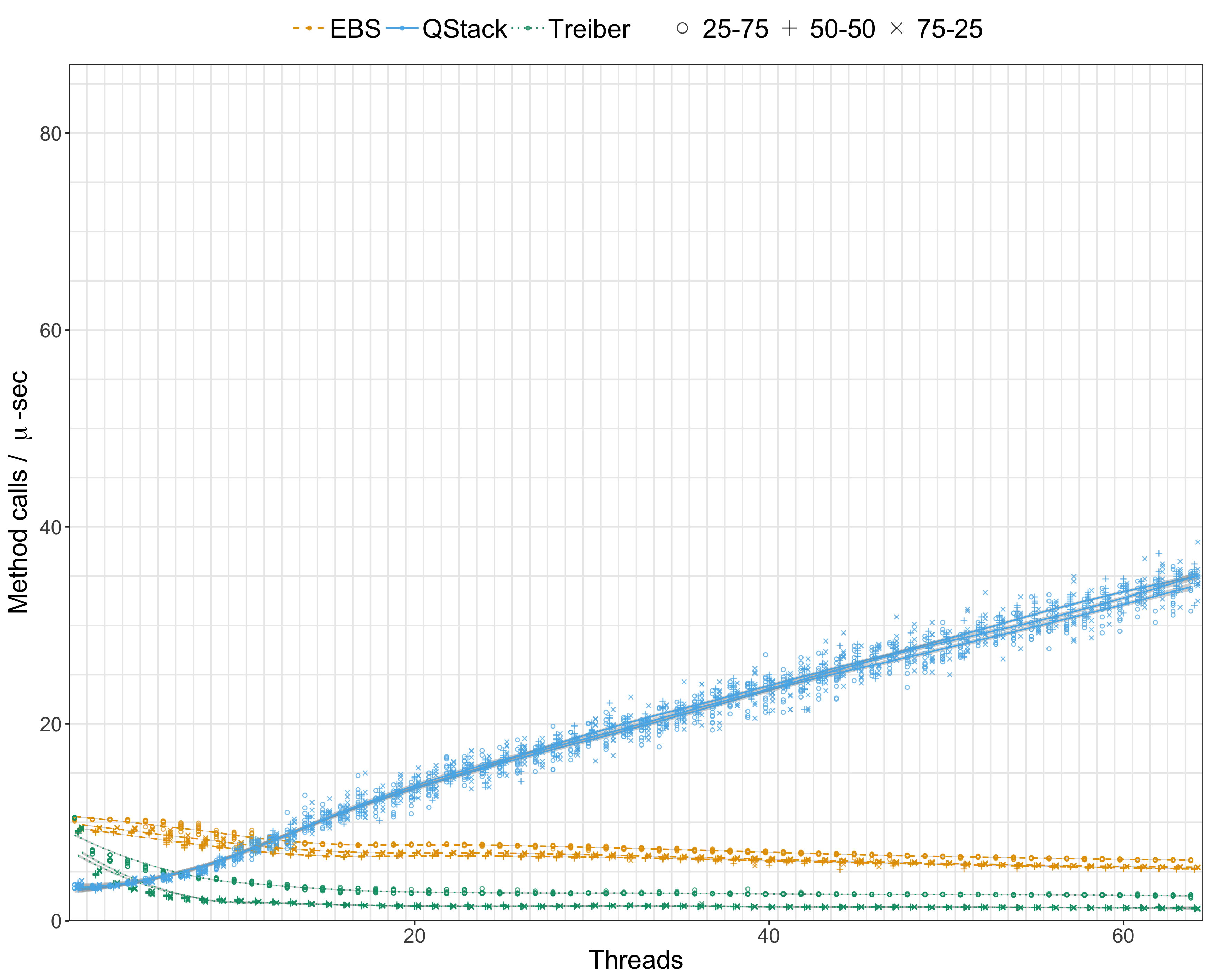
(a) QStack, EBS and Treiber stack.

(b) QQueue, FAA queue, LCRQ and MS queue.

Figure 2. Performance Analysis on the AMD^® EPYC^® server

Experiments were run on an AMD^® EPYC^® server of 2GHz clock speed and 128GB memory, with 32 cores delivering a maximum of 64 simultaneous multi-threads. The operating system is Ubuntu 18.04 LTS and code is compiled with gcc 7.3.0 using -O3 optimizations.

The QStack was compared with the lock-free Elimination Backoff Stack (EBS) (Bar-Nissan et al., 2011) and lock-free Treiber Stack (Treiber, 1986). These were selected as representative of a relaxed semantics stack and a classic linearizable stack. With a single thread, Treiber and EBS demonstrate similar performance, while QStack is lower due to the overhead of descriptors, which incur more remote memory accesses. The operations mix made little difference, but the Treiber Stack and EBS showed slightly higher performance at 25-75 because they quickly discard unsatisfied pop calls, returning $null$. As threads are added, Treiber drops off quickly due to contention. At five threads QStack overtakes Treiber and at 12 threads becomes faster than EBS. The salient result is that the QStack continues to scale, achieving over five times EBS performance with 64 threads. The other implementations consume resources to maintain order at microsecond scale instead of serving requests as quickly as possible with best efforts ordering.

Testing methodology follows those used in the original EBS presentation, going from one to 64 threads with five million operations per thread. Memory is pre-allocated in the stack experiments, and for each run the program is restarted by a script to prevent the previous memory state from influencing the next run. The Boost library (Beman Dawes and Rivera, 2018) is used to create a uniform random distribution of method calls based on the different mixes.

Stack $push$-$pop$ mixes of 25-75, 50-50 and 75-25 were tested for each implementation across all threads. Queue $enqueue$-$dequeue$ mixes were temporal variations on a 50-50 mix. For both stack and queue, there were a minimum of 10 trials per thread per mix. The data was smoothed using the LOESS method as implemented in the ggplot2 library. Shaded areas indicate the 95 percent confidence limits for the lines. Additionally, the data points for every run are shown in both stack and queue plots, with slight x-offsets to the left and right inside the column for readability.

The QQueue was compared with the lock-free LCRQ (Morrison and Afek, 2013), the wait-free FAA queue (Yang and Mellor-Crummey, 2016) and the lock-free MS queue (Michael and Scott, 1995). The LCRQ and FAA are the fastest queues in a recent benchmark framework with ACM verified code artifacts (Yang, 2018). The MS queue is a classic like the Treiber stack. The framework uses only 50-50 mixes, one random (50-50) and one pairwise (50PW). The QQueue performs similarly to LCRQ until overtaking it at 14 threads, then overtaking the wait-free FAA queue at 18 threads. The FAA queue is exceptional as it performs as well or better than the alternative lock-free implementations. The TS-Queue (Haas, 2015) and the Multiqueue (Rihani et al., 2015) are queues of interest published more recently than the FAA queue, but were not selected because verified code artifacts have not been published.

Queue experiments follow the methodology of the Yang and Mellor-Crummey framework (Yang, 2018) and use the queue implementations provided in the source code. Memory allocation is dynamic within the framework. Benchmarks provided are two variations on 50-50 mixes, one random and the other pairwise. The different temporal distributions within the 50-50 mix have more influence on the results than different mixes (25-75, 50-50, 75-25) used in the stack experiments.

In both the pairwise and random mixes, the QQueue continues to scale to the limit of hardware support, more than double the performance of FAA and LCRQ at 64 threads.

The quantifiable containers continue to scale until all threads are employed, with slightly reduced slope in the simultaneous multi-threading region from 32 to 64 threads. Other implementations, including those that are linearizable with relaxed semantics, could maintain microscale order only at the cost of scalability. Furthermore, linearizability may cause unfairness where method calls are not conserved. It follows that quantifiability allows for the design of fast and highly scalable multiprocessor data structures for modern multi-core computing platforms.

8.3. Entropy Applied to Concurrent Objects

With a large number of threads and therefore many overlapping method calls, quantifiability and linearizability both accept any ordering of the overlapping calls. The results presented in Section 8.2 show performance gains for prototype quantifiable data structures over their linearizable counterparts. What is missing is a way to measure the disorder introduced to achieve such gains. This section will propose a measure of the disorder and apply it to the experimental results shown in Figure 2(a).

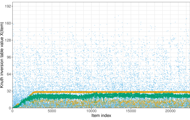
(a) Knuth inversions X(item) 32 threads

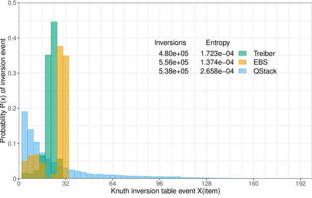
(b) Distribution P(X) of inversions

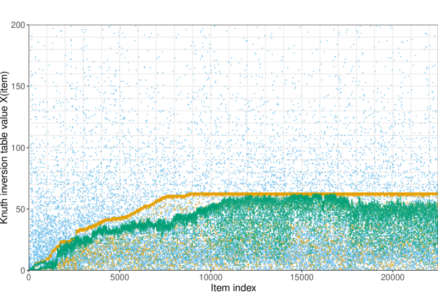
(c) Knuth inversions X(item) 64 threads

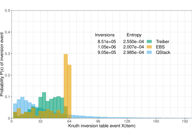
(d) Distribution P(X) of inversions

Figure 3. Inversion events X(item) and distribution P(X) for concurrent stacks, 32 and 64 threads.

Entropy applied to information systems is called Shannon entropy, also referred to as information entropy (Shannon, 1948). Shannon entropy measures the amount of uncertainty in a probability distribution (Goodfellow et al., 2016). With a single process calling a non-concurrent object, the results are completely predictable. Concurrent data structures, even provably linearizable ones, may admit unpredictable results. A perfectly ordered data stream input sequentially to a linearizable FIFO queue will not necessarily emerge in the same order. Overlapping method calls together with the rules of linearizability may allow a great many different correct output orders. In the literature this divergence from the real time order is called an error rate. This term is misleading as it implies failure or incorrectness. Where the unpredictability of a concurrent system is not an error, but lies within the bounds of correctness, we suggest entropy as the measure. In many physical systems, the change in entropy increases with the speed of a reaction. Computing systems cannot escape the general applications of physical laws. The motivation behind generalizing entropy for concurrent objects is to provide the ability to measure the uncertainty in a concurrent system for the comparison of concurrent correctness conditions.

If the natural numbers $1,2...N$ are sent into a FIFO queue and emerge intact, each successive dequeue method call output will always be greater than the preceding dequeue method call output. This scenario represents perfect predictability, and zero entropy. Likewise, a LIFO stack output would perfectly reverse the order. The interesting events are when items come back from our data structures in the “wrong” order. These are called surprises in the literature, and their probability distribution of occurrence is called the surprisal. For an ordered list $a_{1},a_{2},...a_{i}$, an inversion (Knuth, 1998) in the list is a surprise, and the inversion count $x(j)$ is defined for each list element $a_{j}$ as follows:

(2) $$x(j)=count(i<j,a_{i}>a_{j})+count(i>j,a_{i}<a_{j})$$

Given inversion count $x(j)$ defined over the concurrent history with $n$ items, let $k$ be the number of items with an inversion count of $X$. The possible values of $X$ are { $X_{0},...,X_{n}$}. The discrete probability distribution of surprising events is $P(X)=\frac{k}{n}$. The entropy for a set of concurrent histories generated in an experiment is:

(3) $$H(X)=-\sum_{i=0}^{n}P(X_{i})\textnormal{log}P(X_{i})$$

To gather inversion data for the Treiber Stack, EBS and QStack , the real time order of items pushed to the stack was measured using instrumented code as done in (Dodds et al., 2014). The push order was compared to the pop order and inversion events were counted. Raw data points are shown in Figures 3(a), 3(c) and the discrete probability distributions obtained are shown in Figures 3(b), 3(d). It is notable that the Treiber stack and the EBS both show a hard limit on the maximum inversion, being close to the number of threads in each case. This is intuitive for linearizable or near-linearizable data structures because this is the maximum number of overlapping method calls.

At 32 threads, there is some dispersion in the results for Treiber and EBS, but the entropy caused by the QStack is double since there is more uncertainty in method call ordering for the QStack in comparison to the Treiber stack and EBS. At 64 threads, the dispersion is much greater for the EBS and Treiber, and only slightly more for the QStack. The entropy increase reflects this trend since a larger variance in the probability distribution yields higher entropy. Convergence of results at higher thread counts for the concurrent data structures tested is reflected in the similar entropy $P(X)$. The performance results presented in Figure 2(a) showcase how the QStack design leverages the uncertainty in a concurrent system to deliver high scalability obtained through relaxed semantics.

9. Conclusion

Quantifiability is a new concurrent correctness condition compatible with drivers of scalability: architecture, semantics and complexity. Quantifiability is compositional without dependence upon timing or data structure semantics and is free of inherent locking or waiting. The convenient expression of quantifiability in a linear algebra model offers the promise of reduced verification time complexity and powerful abstractions to facilitate concurrent programming innovation. The relaxed semantics permitted by quantifiability allow for significant performance gains through contention avoidance in the implementation of concurrent data structures. Entropy can be applied to evaluate the tradeoff between relaxed semantics and performance.

References

- (1)
- Abelson et al. ([n. d.]) Harold Abelson, Gerald Jay Sussman, and Julie Sussman. [n. d.]. Structure and Interpretation of Computer Programs - 2nd Edition. Justin Kelly.
- Adhikari et al. (2013) Kiran Adhikari, James Street, Chao Wang, Yang Liu, and Shaojie Zhang. 2013. Verifying a Quantitative Relaxation of Linearizability via Refinement. In Model Checking Software, Ezio Bartocci and C R Ramakrishnan (Eds.). Lecture Notes in Computer Science, Vol. 7976. Springer Berlin Heidelberg, Berlin, Heidelberg, 24–42.
- Afek et al. (2010) Yehuda Afek, Guy Korland, and Eitan Yanovsky. 2010. Quasi-Linearizability: Relaxed Consistency for Improved Concurrency. In Principles of Distributed Systems. Springer Berlin Heidelberg, 395–410.
- Alistarh et al. (2018) Dan Alistarh, Trevor Brown, Justin Kopinsky, Jerry Z Li, and Giorgi Nadiradze. 2018. Distributionally Linearizable Data Structures. In Proceedings of the 30th on Symposium on Parallelism in Algorithms and Architectures. ACM, 133–142.
- Alur et al. (1996) R Alur, K McMillan, and D Peled. 1996. Model-checking of correctness conditions for concurrent objects. In Proceedings 11th Annual IEEE Symposium on Logic in Computer Science. 219–228.
- Amit et al. (2007) Daphna Amit, Noam Rinetzky, Thomas Reps, Mooly Sagiv, and Eran Yahav. 2007. Comparison Under Abstraction for Verifying Linearizability. In Computer Aided Verification, Werner Damm and Holger Hermanns (Eds.). Lecture Notes in Computer Science, Vol. 4590. Springer Berlin Heidelberg, Berlin, Heidelberg, 477–490.
- Aspnes et al. (1994) James Aspnes, Maurice Herlihy, and Nir Shavit. 1994. Counting networks. Journal of the ACM (JACM) 41, 5 (1994), 1020–1048.
- Badrinath and Ramamritham (1987) B R Badrinath and K Ramamritham. 1987. Semantics-based concurrency control: Beyond commutativity. In 1987 IEEE Third International Conference on Data Engineering. 304–311.
- Baier and Katoen (2008) Christel Baier and Joost-Pieter Katoen. 2008. Principles of Model Checking. MIT Press.
- Bar-Nissan et al. (2011) Gal Bar-Nissan, Danny Hendler, and Adi Suissa. 2011. A Dynamic Elimination-Combining Stack Algorithm. In Principles of Distributed Systems, Antonio Fernàndez Anta, Giuseppe Lipari, and Matthieu Roy (Eds.). Lecture Notes in Computer Science, Vol. 7109. Springer Berlin Heidelberg, Berlin, Heidelberg, 544–561.
- Bäumler et al. (2011) Simon Bäumler, Gerhard Schellhorn, Bogdan Tofan, and Wolfgang Reif. 2011. Proving linearizability with temporal logic. Form. Asp. Comput. 23, 1 (Jan. 2011), 91–112.
- Beezer (2008) Robert Arnold Beezer. 2008. A first course in linear algebra. Beezer.
- Beman Dawes and Rivera (2018) David Abrahams Beman Dawes and Rene Rivera. 2018. Boost C++ Libraries. https://www.boost.org/users/history/version_1_69_0.html. (Dec. 2018). Accessed: 2019-1-15.
- Best and Randell (1981) Eike Best and Brian Randell. 1981. A formal model of atomicity in asynchronous systems. Acta informatica 16, 1 (1981), 93–124.
- Bouajjani et al. (2015) Ahmed Bouajjani, Michael Emmi, Constantin Enea, and Jad Hamza. 2015. Tractable refinement checking for concurrent objects. Proceedings of the 42nd Annual ACM SIGPLAN-SIGACT Symposium on Principles of Programming Languages (POPL ’15) 50, 1 (2015), 651–662.
- Bouajjani et al. (2017) Ahmed Bouajjani, Michael Emmi, Constantin Enea, and Suha Orhun Mutluergil. 2017. Proving Linearizability Using Forward Simulations. In Computer Aided Verification, Rupak Majumdar and Viktor Kunčak (Eds.). Lecture Notes in Computer Science, Vol. 10427. Springer International Publishing, Cham, 542–563.
- Burckhardt et al. (2010) Sebastian Burckhardt, Chris Dern, Madanlal Musuvathi, and Roy Tan. 2010. Line-up: a complete and automatic linearizability checker. Proceedings of the 31st ACM SIGPLAN Conference on Programming Language Design and Implementation (PLDI’10) 45, 6 (2010), 330–340.
- Chockler et al. (2005) Gregory Chockler, Nancy Lynch, Sayan Mitra, and Joshua Tauber. 2005. Proving atomicity: An assertional approach. In International Symposium on Distributed Computing. Springer, 152–168.
- Debals and De Lathauwer (2015) Otto Debals and Lieven De Lathauwer. 2015. Stochastic and deterministic tensorization for blind signal separation. In International Conference on Latent Variable Analysis and Signal Separation. Springer, 3–13.
- Dechev et al. (2006) Damian Dechev, Peter Pirkelbauer, and Bjarne Stroustrup. 2006. Lock-Free Dynamically Resizable Arrays. In Principles of Distributed Systems. Springer Berlin Heidelberg, 142–156.
- Derrick et al. (2014) John Derrick, Brijesh Dongol, Gerhard Schellhorn, Bogdan Tofan, Oleg Travkin, and Heike Wehrheim. 2014. Quiescent Consistency: Defining and Verifying Relaxed Linearizability. In FM 2014: Formal Methods. Springer International Publishing, 200–214.
- Derrick et al. (2007) John Derrick, Gerhard Schellhorn, and Heike Wehrheim. 2007. Proving Linearizability Via Non-atomic Refinement. In Integrated Formal Methods, Jim Davies and Jeremy Gibbons (Eds.). Lecture Notes in Computer Science, Vol. 4591. Springer Berlin Heidelberg, Berlin, Heidelberg, 195–214.
- Derrick et al. (2011) John Derrick, Gerhard Schellhorn, and Heike Wehrheim. 2011. Verifying Linearisability with Potential Linearisation Points. In FM 2011: Formal Methods. Springer Berlin Heidelberg, 323–337.
- Descartes (1903) René Descartes. 1903. The Meditations, and Selections from the Principles of René Descartes (1596-1650). Open Court.
- Dodds et al. (2014) Mike Dodds, Andreas Haas, and Christoph M Kirsch. 2014. Fast concurrent data-structures through explicit timestamping. Department of Computer Sciences, Universitt Salzburg, Tech. Rep 3 (2014).
- Elmas et al. (2010) Tayfun Elmas, Shaz Qadeer, Ali Sezgin, Omer Subasi, and Serdar Tasiran. 2010. Simplifying Linearizability Proofs with Reduction and Abstraction. In Tools and Algorithms for the Construction and Analysis of Systems, Javier Esparza and Rupak Majumdar (Eds.). Lecture Notes in Computer Science, Vol. 6015. Springer Berlin Heidelberg, Berlin, Heidelberg, 296–311.
- Emmi and Enea (2017) Michael Emmi and Constantin Enea. 2017. Sound, complete, and tractable linearizability monitoring for concurrent collections. Proceedings of the ACM on Programming Languages 2, POPL (Dec. 2017), 25.
- Emmi et al. (2015) Michael Emmi, Constantin Enea, and Jad Hamza. 2015. Monitoring refinement via symbolic reasoning. In Proceedings of the 36th ACM SIGPLAN Conference on Programming Language Design and Implementation (PLDI ’15), Vol. 50. ACM, 260–269.
- Feldman et al. (2018) Yotam M Y Feldman, Constantin Enea, Adam Morrison, Noam Rinetzky, and Sharon Shoham. 2018. Order out of Chaos: Proving Linearizability Using Local Views. (May 2018). arXiv:cs.DC/1805.03992
- Flanagan et al. (2004) Cormac Flanagan, Cormac Flanagan, and Stephen N Freund. 2004. Atomizer: a dynamic atomicity checker for multithreaded programs. In Proceedings of the 31st ACM SIGPLAN-SIGACT symposium on Principles of programming languages, Vol. 39. ACM, 256–267.
- Flanagan et al. (2008) Cormac Flanagan, Stephen N Freund, and Jaeheon Yi. 2008. Velodrome: a sound and complete dynamic atomicity checker for multithreaded programs. Proceedings of the 29th ACM SIGPLAN Conference on Programming Language Design and Implementation 43, 6 (2008), 293–303.
- Flanagan and Godefroid (2005) Cormac Flanagan and Patrice Godefroid. 2005. Dynamic partial-order reduction for model checking software. In Proceedings of the 32nd ACM SIGPLAN-SIGACT symposium on Principles of programming languages, Vol. 40. ACM, 110–121.
- Flanagan and Qadeer (2003) Cormac Flanagan and Shaz Qadeer. 2003. A type and effect system for atomicity. In Proceedings of the ACM SIGPLAN 2003 conference on Programming language design and implementation, Vol. 38. ACM, 338–349.
- Gogolla et al. (1984) M Gogolla, K Drosten, U Lipeck, and H-D Ehrich. 1984. Algebraic and operational semantics of specifications allowing exceptions and errors. Theor. Comput. Sci. 34, 3 (Jan. 1984), 289–313.
- Goodfellow et al. (2016) Ian Goodfellow, Yoshua Bengio, and Aaron Courville. 2016. Deep Learning. MIT Press. http://www.deeplearningbook.org.
- Grasedyck (2010) Lars Grasedyck. 2010. Polynomial approximation in hierarchical Tucker format by vector-tensorization. Inst. für Geometrie und Praktische Mathematik.
- Gruber et al. (2016) Jakob Gruber, Jesper Larsson Träff, and Martin Wimmer. 2016. Benchmarking Concurrent Priority Queues: Performance of k-LSM and Related Data Structures. (March 2016). arXiv:cs.DS/1603.05047
- Guerraoui et al. (2012) Rachid Guerraoui, Viktor Kuncak, and Giuliano Losa. 2012. Speculative Linearizability. In Proceedings of the 33rd ACM SIGPLAN Conference on Programming Language Design and Implementation (PLDI ’12). ACM, New York, NY, USA, 55–66.
- Guttag (1976) John Guttag. 1976. Abstract data types and the development of data structures. In Proceedings of the 1976 conference on Data : Abstraction, definition and structure, Vol. 11. ACM, 72.
- Guttag et al. (1978) John V Guttag, Ellis Horowitz, and David R Musser. 1978. Abstract data types and software validation. Commun. ACM 21, 12 (1978), 1048–1064.
- Haas (2015) A Haas. 2015. Fast concurrent data structures through timestamping. Ph.D. Dissertation. PhD thesis, University of Salzburg, Salzburg, Austria.
- Haas et al. (2013) Andreas Haas, Michael Lippautz, Thomas A Henzinger, Hannes Payer, Ana Sokolova, Christoph M Kirsch, and Ali Sezgin. 2013. Distributed Queues in Shared Memory: Multicore Performance and Scalability Through Quantitative Relaxation. In Proceedings of the ACM International Conference on Computing Frontiers (CF ’13). ACM, New York, NY, USA, 17:1–17:9.
- Harris et al. (2002) Timothy L Harris, Keir Fraser, and Ian A Pratt. 2002. A practical multi-word compare-and-swap operation. In International Symposium on Distributed Computing. Springer, 265–279.
- Hendler et al. (2004) Danny Hendler, Nir Shavit, and Lena Yerushalmi. 2004. A Scalable Lock-free Stack Algorithm. In Proceedings of the Sixteenth Annual ACM Symposium on Parallelism in Algorithms and Architectures (SPAA ’04). ACM, New York, NY, USA, 206–215.
- Henzinger et al. (2013) Thomas A Henzinger, Christoph M Kirsch, Hannes Payer, Ali Sezgin, and Ana Sokolova. 2013. Quantitative Relaxation of Concurrent Data Structures. In Proceedings of the 40th Annual ACM SIGPLAN-SIGACT Symposium on Principles of Programming Languages (POPL ’13). ACM, New York, NY, USA, 317–328.
- Herlihy (1991) Maurice Herlihy. 1991. Wait-free Synchronization. ACM Trans. Program. Lang. Syst. 13, 1 (Jan. 1991), 124–149.
- Herlihy and Shavit (2012) Maurice Herlihy and Nir Shavit. 2012. The Art of Multiprocessor Programming. Morgan Kaufmann. Revised Reprint. ISBN: 0123973375.
- Herlihy and Wing (1990a) Maurice P Herlihy and Jeannette M Wing. 1990a. Linearizability: A correctness condition for concurrent objects. ACM Transactions on Programming Languages and Systems (TOPLAS) 12, 3 (1990), 463–492.
- Herlihy and Wing (1990b) Maurice P Herlihy and Jeannette M Wing. 1990b. Linearizability: A Correctness Condition for Concurrent Objects. ACM Trans. Program. Lang. Syst. 12, 3 (July 1990), 463–492.
- Hoare (1978) Charles Antony Richard Hoare. 1978. Proof of correctness of data representations. In Programming Methodology. Springer, 269–281.
- Khyzha et al. (2017) Artem Khyzha, Mike Dodds, Alexey Gotsman, and Matthew Parkinson. 2017. Proving Linearizability Using Partial Orders. In Programming Languages and Systems. Springer Berlin Heidelberg, 639–667.
- Khyzha et al. (2016) Artem Khyzha, Alexey Gotsman, and Matthew Parkinson. 2016. A Generic Logic for Proving Linearizability. In FM 2016: Formal Methods, John Fitzgerald, Constance Heitmeyer, Stefania Gnesi, and Anna Philippou (Eds.). Lecture Notes in Computer Science, Vol. 9995. Springer International Publishing, Cham, 426–443.
- Kirsch et al. (2013) Christoph M Kirsch, Michael Lippautz, and Hannes Payer. 2013. Fast and scalable, lock-free k-FIFO queues. In International Conference on Parallel Computing Technologies. Springer, 208–223.
- Knuth (1998) Donald E Knuth. 1998. The Art of Computer Programming: Volume 3: Sorting and Searching. Addison-Wesley Professional.
- Kogan and Petrank (2012) Alex Kogan and Erez Petrank. 2012. A methodology for creating fast wait-free data structures. In Proceedings of the 17th ACM SIGPLAN symposium on Principles and Practice of Parallel Programming, Vol. 47. ACM, 141–150.
- Lamport (1978) Leslie Lamport. 1978. Time, clocks, and the ordering of events in a distributed system. Commun. ACM 21, 7 (July 1978), 558–565.
- Lamport (1979) Leslie Lamport. 1979. How to make a multiprocessor computer that correctly executes multiprocess program. IEEE Trans. Comput. 9 (1979), 690–691.
- Liang and Feng (2013) Hongjin Liang and Xinyu Feng. 2013. Modular Verification of Linearizability with Non-fixed Linearization Points. SIGPLAN Not. 48, 6 (June 2013), 459–470.
- Lipton (1975) Richard J Lipton. 1975. Reduction: A method of proving properties of parallel programs. Commun. ACM 18, 12 (1975), 717–721.
- Liskov and Wing (1994) Barbara H Liskov and Jeannette M Wing. 1994. A Behavioral Notion of Subtyping. ACM Trans. Program. Lang. Syst. 16, 6 (Nov. 1994), 1811–1841.
- Michael and Scott (1995) M M Michael and M L Scott. 1995. Simple, Fast, and Practical Non-Blocking and Blocking Concurrent Queue Algorithms. Technical Report 600 (1995).
- Morrison and Afek (2013) A Morrison and Y Afek. 2013. Fast concurrent queues for x86 processors. Proceedings of the 18th ACM SIGPLAN symposium on Principles and practice of parallel programming (2013).
- Nanevski et al. (2019) Aleksandar Nanevski, Anindya Banerjee, Germán Andrés Delbianco, and Ignacio Fábregas. 2019. Specifying Concurrent Programs in Separation Logic: Morphisms and Simulations. arXiv preprint arXiv:1904.07136 (2019).
- National Research Council et al. (2011) National Research Council, Division on Engineering and Physical Sciences, Computer Science and Telecommunications Board, and Committee on Sustaining Growth in Computing Performance. 2011. The Future of Computing Performance: Game Over or Next Level? National Academies Press.
- O’Hearn et al. (2010) Peter W O’Hearn, Noam Rinetzky, Martin T Vechev, Eran Yahav, and Greta Yorsh. 2010. Verifying Linearizability with Hindsight. In Proceedings of the 29th ACM SIGACT-SIGOPS Symposium on Principles of Distributed Computing (PODC ’10). ACM, New York, NY, USA, 85–94.
- Ou and Demsky (2017) Peizhao Ou and Brian Demsky. 2017. Checking concurrent data structures under the C/C++ 11 memory model. In Proceedings of the 22nd ACM SIGPLAN Symposium on Principles and Practice of Parallel Programming (PPoPP ’17), Vol. 52. ACM, 45–59.
- Papadimitriou (1979) Christos H Papadimitriou. 1979. The serializability of concurrent database updates. Journal of the ACM (JACM) 26, 4 (1979), 631–653.
- Rihani et al. (2015) Hamza Rihani, Peter Sanders, and Roman Dementiev. 2015. Brief Announcement: MultiQueues: Simple Relaxed Concurrent Priority Queues. In Proceedings of the 27th ACM Symposium on Parallelism in Algorithms and Architectures (SPAA ’15). ACM, New York, NY, USA, 80–82. https://doi.org/10.1145/2755573.2755616
- Schellhorn et al. (2014) Gerhard Schellhorn, John Derrick, and Heike Wehrheim. 2014. A Sound and Complete Proof Technique for Linearizability of Concurrent Data Structures. ACM Trans. Comput. Log. 15, 4 (Sept. 2014), 31:1–31:37.
- Scherer and Scott (2004) William N Scherer and Michael L Scott. 2004. Nonblocking concurrent data structures with condition synchronization. In International Symposium on Distributed Computing. Springer, 174–187.
- Sergey et al. (2016) Ilya Sergey, Aleksandar Nanevski, Anindya Banerjee, and Germán Andrés Delbianco. 2016. Hoare-style specifications as correctness conditions for non-linearizable concurrent objects. Proceedings of the 2016 ACM SIGPLAN International Conference on Object-Oriented Programming, Systems, Languages, and Applications (OOPSLA ’16) 51, 10 (2016), 92–110.
- Shacham et al. (2011) Ohad Shacham, Nathan Bronson, Alex Aiken, Mooly Sagiv, Martin Vechev, and Eran Yahav. 2011. Testing atomicity of composed concurrent operations. In Proceedings of the 2011 ACM international conference on Object oriented programming systems languages and applications, Vol. 46. ACM, 51–64.
- Shannon (1948) Claude Elwood Shannon. 1948. A mathematical theory of communication. Bell system technical journal 27, 3 (1948), 379–423.
- Shavit (2011) Nir Shavit. 2011. Data structures in the multicore age. Commun. ACM 54, 3 (March 2011), 76–84.
- Shavit and Taubenfeld (2015) Nir Shavit and Gadi Taubenfeld. 2015. The Computability of Relaxed Data Structures: Queues and Stacks as Examples. In Structural Information and Communication Complexity, Christian Scheideler (Ed.). Lecture Notes in Computer Science, Vol. 9439. Springer International Publishing, Cham, 414–428.
- Sheehy (2015) Justin Sheehy. 2015. There is no now. (2015), 36–41 pages.
- Singh et al. (2016) V Singh, I Neamtiu, and R Gupta. 2016. Proving Concurrent Data Structures Linearizable. In 2016 IEEE 27th International Symposium on Software Reliability Engineering (ISSRE). 230–240.
- Strachey (1967) C. S. Strachey. 1967. Fundamental Concepts of Programming Languages. Programming Research Group.
- Stroustrup (2013) Bjarne Stroustrup. 2013. The C++ Programming Language (4th Ed.). Pearson Education.
- Tofan et al. (2014) Bogdan Tofan, Oleg Travkin, Gerhard Schellhorn, and Heike Wehrheim. 2014. Two approaches for proving linearizability of multiset. Science of Computer Programming 96 (Dec. 2014), 297–314.
- Treiber (1986) R Kent Treiber. 1986. Systems programming: Coping with parallelism. International Business Machines Incorporated, Thomas J. Watson Research Center New York.
- Vechev et al. (2009) Martin Vechev, Eran Yahav, and Greta Yorsh. 2009. Experience with model checking linearizability. In International SPIN Workshop on Model Checking of Software. Springer, 261–278.
- Wen et al. (2018) Tangliu Wen, Lan Song, and Zhen You. 2018. Proving Linearizability Using Reduction. Comput. J. (Nov. 2018).
- Williams et al. (2007) Samuel Williams, Leonid Oliker, Richard Vuduc, John Shalf, Katherine Yelick, and James Demmel. 2007. Optimization of sparse matrix-vector multiplication on emerging multicore platforms. In SC’07: Proceedings of the 2007 ACM/IEEE Conference on Supercomputing. IEEE, 1–12.
- Wimmer et al. (2015) Martin Wimmer, Jakob Gruber, Jesper Larsson Träff, and Philippas Tsigas. 2015. The Lock-free k-LSM Relaxed Priority Queue. In Proceedings of the 20th ACM SIGPLAN Symposium on Principles and Practice of Parallel Programming (PPoPP 2015). ACM, New York, NY, USA, 277–278.
- Wing (1989) Jeannette M Wing. 1989. Verifying atomic data types. International Journal of Parallel Programming 18, 5 (1989), 315–357.
- Yang (2018) Chaoran Yang. 2018. Fast Wait Free Queue. https://github.com/chaoran/fast-wait-free-queue. (Oct. 2018). Accessed: 2019-2-5.
- Yang and Mellor-Crummey (2016) Chaoran Yang and John Mellor-Crummey. 2016. A wait-free queue as fast as fetch-and-add. In Proceedings of the 21st ACM SIGPLAN Symposium on Principles and Practice of Parallel Programming - PPoPP ’16. ACM Press, New York, New York, USA, 1–13.
- Zaremski and Wing (1995) Amy Moormann Zaremski and Jeannette M Wing. 1995. Specification Matching of Software Components. In Proceedings of the 3rd ACM SIGSOFT Symposium on Foundations of Software Engineering (SIGSOFT ’95). ACM, New York, NY, USA, 6–17.
- Zhang et al. (2015) Lu Zhang, Arijit Chattopadhyay, and Chao Wang. 2015. Round-up: runtime verification of quasi linearizability for concurrent data structures. IEEE Transactions On Software Engineering 41, 12 (2015), 1202–1216.