A Distributed Incremental Update Scheme for Probability Distribution of Wind Power Forecast Error

^†Department of Electrical Engineering, Tsinghua University, Beijing 100084, China

^⋆State Key Laboratory of Power Systems, Beijing 100084, China

^⋄Author for Correspondence: shenchen@mail.tsinghua.edu.cn

Abstract: Due to the uncertainty of distributed wind generations (DWGs), a better understanding of the probability distributions (PD) of their wind power forecast errors (WPFEs) can help market participants (MPs) who own DWGs perform better during trading. Under the premise of an accurate PD model, considering the correlation among DWGs and absorbing the new information carried by the latest data are two ways to maintain an accurate PD. These two ways both require the historical and latest wind power and forecast data of all DWGs. Each MP, however, only has access to the data of its own DWGs and may refuse to share these data with MPs belonging to other stakeholders. Besides, because of the endless generation of new data, the PD updating burden increases sharply. Therefore, we use the distributed strategy to deal with the data collection problem. In addition, we further apply the incremental learning strategy to reduce the updating burden. Finally, we propose a distributed incremental update scheme to make each MP continually acquire the latest conditional PD of its DWGs’ WPFE. Specifically, we first use the Gaussian-mixture-model-based (GMM-based) joint PD to characterize the correlation among DWGs. Then, we propose a distributed modified incremental GMM algorithm to enable MPs to update the parameters of the joint PD in a distributed and incremental manner. After that, we further propose a distributed derivation algorithm to make MPs derive their conditional PD of WPFE from the joint one in a distributed way. Combining the two original algorithms, we finally achieve the complete distributed incremental update scheme, by which each MP can continually obtain its latest conditional PD of its DWGs’ WPFE via neighborhood communication and local calculation with its own data. The effectiveness, correctness, and efficiency of the proposed scheme are verified using the dataset from the NREL.

Keywords: Distributed wind generation, Prosumer, Wind power forecast error, Probability distribution, Incremental learning, Distributed

1. Introduction

Significantly increasing development of distributed renewable energy (DRE) allows traditionally passive consumers to become ‘prosumers’ under consumer level communications and control [1]. Accordingly, different trading schemes have emerged to incentivise prosumers to participate in local markets, e.g., peer-to-peer scheme [2] and aggregator scheme [3]. No matter which scheme market participants (MPs) choose, they have to face the uncertainty brought by their DREs [4]. Since generating a perfect forecast remains a challenge under current technologies [5], a better understanding of the probability distribution (PD) of the DRE forecast error can help these MPs perform better in storage system arrangement [6] and bidding strategy selection [7]. In this paper, we focus on distributed wind generation (DWG) and aim to make each MP obtain an accurate PD of its DWGs’ forecast error.

There are two ideas that can help MPs build and maintain an accurate PD of wind power forecast error (WPFE). One is considering the wind power correlation among DWGs when building the PD. Another one is updating the established PD in real time by absorbing new information carried by new data. It should be emphasized that, knowing the wind power forecast values of all DWGs may assist each MP to build a more accurate distribution than the one it individually creates with its own data [8]. Therefore, each MP should first build the joint PD of all DWGs’ wind power and forecast data. Then, each MP should derive the conditional PD of its DWGs’ WPFE under all DWGs’ latest forecast values from the joint one [9, 10, 11]. Meanwhile, each MP should update its conditional PD when new wind power and forecast data emerge. The prerequisite of the two ideas is that each MP can always have access to the historical and latest wind power and forecast data of all DWGs. The fact, however, is that each MP only has access to the data of its own DWGs. As the bidding of DWGs is dependent on their forecast values, MPs may refuse to share these data with MPs belonging to other stakeholders. To avoid the data collection, a distributed strategy is a feasible choice. Except for the problem of data collection, each MP also faces the high calculation burden when updating the conditional PD due to the endless increase in new data. To solve the two problems, this paper aims to develop an efficient distributed update scheme to make each MP obtain the latest conditional PD of its DWGs’ WPFE. For the sake of brevity, we will hereinafter use this phrase, ‘each MP’s conditional PD of WPFE’, to represent each MP’s conditional PD of its DWGs’ WPFE when it does not cause ambiguity.

A suitable distribution model is the basis of the scheme. Many efforts have been made to model the PD of the WPFE. A common approach is to represent the WPFE as a normally distributed random variable with the forecast value as the expected value [12]. The Weibull distribution, beta distribution [7], and Cauchy distribution [13] are other common models for characterizing the uncertainty of the WPFE. However, the Gaussian, beta, and Cauchy distributions are not universal, particularly when the time scales change [14]. Other modified models, e.g., the Levy alpha-stable distribution [15], mixed beta distribution [16], Gamma-like distribution [17], and t-location distribution [18], have also been proposed to better fit the features of the WPFE. Subsequently, to improve the generality of the PD model, researchers have tended to utilize or develop models that have more adjustable parameters. Zhang et al. presented a versatile distribution with three adjustable shape parameters estimated by nonlinear least-squares [5, 19], which not only can better represent the WPFE than the Gaussian and beta distributions [5] but also has analytical forms of the cumulative distribution function (CDF) and its inverse function. However, the unimodal feature of the versatile distribution limits its application [20]. An improved versatile distribution with a more accurate representation was first proposed to solve this problem. Then, a versatile mixture distribution was developed through the convex combination of several improved versatile distributions [20]. Recently, the Gaussian mixture model (GMM) has been applied to stochastic analyses of power systems because it can characterize multidimensional random variables subject to an arbitrary distribution with high precision regardless of the timescale [21, 22, 23]. Meanwhile, the GMM makes it easy to derive the conditional PD from the GMM-based joint PD because of its highly analytical feature [11, 24]. Thus, many researchers use GMM to represent the conditional PD of the WPFE [9, 10, 11]. The GMM is also adopted in this paper.

The expectation–maximization (EM) algorithm is the most commonly used method to estimate the parameters of the GMM [21, 22]. This algorithm needs to collect the historical wind power and wind power forecast data of the correlated DWGs and train them. However, as an offline training method, this algorithm requires a complete historical dataset for each training. As new data continue to emerge, the size of the historical dataset increases, resulting in a sharply increasing update cost. To realize an efficient update scheme, the incremental learning algorithm is a feasible method. As a dynamic technique in machine learning, the incremental learning algorithm can learn new knowledge only from new data and keep most of the knowledge that has been learned before, thus avoiding the repeated training of old data and improving the efficiency. For updating the parameters in the GMM, incremental learning algorithms have been investigated in the fields of video recognition, robot control, etc. [25, 26, 27, 28, 29, 30, 31, 32]. The research on incremental learning algorithms can be divided into two types: (1) block-wise incremental learning algorithms [25, 26, 27] and (2) point-wise incremental learning algorithms [28, 29, 30, 31, 32]. The former updates the GMM after a certain amount of new data has been generated, while the latter updates GMM point by point when a piece of new data is generated. The key to the block-wise incremental learning algorithm lies in whether and how to merge the two GMMs built by the old dataset and the new dataset. Merging judgments include the statistical feature equivalence judgment [25], fidelity judgment [26] and Kullback-Leibler divergence judgment [27], and the merging operations are based on weighted fusion. Since the block-wise incremental learning algorithm requires waiting for the generation of a certain amount of new data, the updating may not be timely. Therefore, the point-wise incremental learning algorithm is a better choice. The point-wise incremental learning algorithm generally consists of 3 steps: the judging step, updating step, and creating step. The first step is to decide whether a piece of new data belongs to an existing Gaussian component in the GMM. Different criteria are utilized: the likelihood value of a component when substituting the latest data in it [30], the distance between the latest data and the expected value of the components [29], or the Mahalanobis distance between the latest data and the components [28, 31, 32]. If the judgment passed, i.e., the new data belongs to an existing Gaussian component, then the parameters of the GMM will be updated based on the new data in the second step. The Robbins-Monro stochastic approximation method is the most common method to estimate the updated parameters of the GMM [30] and is improved in [31, 32] by introducing the inverse of the covariance to avoid the need for the inverse calculation in each update. The filter-based algorithms, i.e., the causal low-pass filter [29] and self-adapted recursive filter [28], are also used to update the parameters. If the judgment is not passed, then a new Gaussian component is created [30, 31, 32], or the less contributing component is replaced [28] in the third step with a preset covariance and a mean vector equal to the new data.

Among the above point-wise incremental learning algorithms, we choose the commonly used modified incremental GMM (IGMM) algorithm [31] to realize an incremental update scheme for the GMM-based PD. This scheme, however, still needs to collect the continuously new wind power and forecast data from all DWGs. To deal with the data barriers among MPs, we should further adapt the incremental update scheme into a distributed one. Specifically, a distributed modified IGMM algorithm is first needed for updating the parameters of the GMM-based joint PD. Then, a distributed derivation algorithm is also required to derive the conditional PD from the updated joint PD under the current wind power forecast value of all DWGs. The distributed point-wise incremental learning algorithm and distributed derivation algorithm compose a complete distributed incremental update scheme.

To the best of our knowledge, neither the distributed point-wise incremental learning algorithm, the distributed derivation algorithm, or the final distributed incremental update scheme have previously been reported. Therefore, in this paper, we aim to propose this distributed incremental update scheme to update each MP’s conditional PD of WPFE. The original contributions of this paper are as follows:

• We propose a distributed framework for the modified IGMM algorithm. Based on this framework, we further develop a distributed modified IGMM algorithm. This algorithm can enable each MP to efficiently update the parameters of the joint PD when new data arrives.

• We propose a distributed framework for the derivation process of the conditional PD. According to this framework, we further design a distributed derivation algorithm. This algorithm can enable each MP to derive the conditional PDs of WPFE under all DWGs’ latest forecast values from the joint PD.

• We develop a distributed incremental update scheme by combining the above two original algorithms. This scheme is fully distributed and can keep each MP’s conditional PDs of WPFE stay up to date with extremely low and stable update costs regardless of how much the historical dataset grows.

The remainder of this paper is organized as follows. In Section 2, the GMM-based joint PD and conditional PD of the WPFE are provided. The distributed framework for the derivation process of the conditional PD is formulated in Section 3. In Section 4, the distributed framework for the modified IGMM algorithm is formulated. The distributed modified IGMM algorithm, the distributed derivation algorithm, and the distributed incremental update scheme are proposed in Section 5. Case studies are performed in Section 6. Finally, Section 7 concludes this paper.

2. GMM-based Probability Distribution

In this section, the joint PD for correlated DWGs is first introduced. Then, the derivation for the conditional PD of the WPFE from the joint PD is presented.

2.1 Joint Probability Distribution

We assume that the number of MPs is M. Besides, each MP owns one DWG. Denote the wind power, wind power forecast and WPFE of the MPs by random vectors $\bm{X},\bm{Y},\bm{Z}\in\mathbb{R}^{M}$, respectively, where $\bm{Z}=\bm{X}-\bm{Y}$. The m-th elements of $\bm{X}$, $\bm{Y}$ and $\bm{Z}$, i.e., $\bm{x}_{m}$, $\bm{y}_{m}$ and $\bm{z}_{m}$, represent the wind power, wind power forecast and WPFE of the m-th MP. The GMM-based joint PD of $\bm{X}$ and $\bm{Y}$ with J Gaussian components is given in (1):

$$P({\mathbf{X}},{\mathbf{Y}})=\sum_{j=1}^{J}w_{j}\mathcal{N}_{j}({\mathbf{X}},{\mathbf{Y}})=\sum_{j=1}^{J}w_{j}\mathcal{N}_{j}(\mathbf{U};\bm{\mu}_{j},\bm{\Sigma}_{j})$$ (1)

$$\mathcal{N}_{j}(\mathbf{U};\bm{\mu}_{j},\bm{\Sigma}_{j})=\frac{exp[-\frac{1}{2}(\mathbf{U}-\bm{\mu}_{j})\bm{\Sigma}_{j}^{-1}(\mathbf{U}-\bm{\mu}_{j})^{T}]}{\sqrt{(2\pi)^{2M}det(\bm{\Sigma}_{j})}}$$ (2)

where $\mathcal{N}_{j}(\cdot)$ is the j-th 2M-dimensional Gaussian distribution as in (2) with a weighted coefficient $w_{j}$, a mean vector $\bm{\mu}_{j}\in\mathbb{R}^{2M}$ and a covariance matrix $\bm{\Sigma}_{j}\in\mathbb{R}^{2M\times 2M}$. $\bm{U}$ is the compact form of $[\bm{X},\bm{Y}]$. The parameter set of the joint PD is defined as $\bm{\theta}=\{w_{j},\bm{\mu}_{j},\bm{\Sigma}_{j}|j=1,2,...,J\}$, where the details of $\bm{\mu}_{j}$ and $\bm{\Sigma}_{j}$ are provided in (3) – (7).

$$\bm{\mu}_{j}=\begin{bmatrix}\bm{\mu}_{j,x}&\bm{\mu}_{j,y}\end{bmatrix},\ \bm{\mu}_{j,x}=\begin{bmatrix}\mu_{j,x_{1}}&\cdots&\mu_{j,x_{M}}\end{bmatrix}$$ (3)

$$\bm{\mu}_{j,y}=\begin{bmatrix}\mu_{j,y_{1}}&\cdots&\mu_{j,y_{M}}\end{bmatrix},\ \bm{\Sigma}_{j}=\begin{bmatrix}\bm{A}_{j}&\bm{B}_{j}\\ \bm{B}_{j}^{T}&\bm{C}_{j}\end{bmatrix}$$ (4)

$$\bm{A}_{j}=\begin{bmatrix}\sigma_{j,x_{1},x_{1}}&\cdots&\sigma_{j,x_{1},x_{M}}\\ \vdots&\ddots&\vdots\\ \sigma_{j,x_{M},x_{1}}&\cdots&\sigma_{j,x_{M},x_{M}}\end{bmatrix}$$ (5)

$$\bm{B}_{j}=\begin{bmatrix}\sigma_{j,x_{1},y_{1}}&\cdots&\sigma_{j,x_{1},y_{M}}\\ \vdots&\ddots&\vdots\\ \sigma_{j,x_{M},y_{1}}&\cdots&\sigma_{j,x_{M},y_{M}}\end{bmatrix}=\begin{bmatrix}\bm{b}_{j,1}\\ \vdots\\ \bm{b}_{j,M}\end{bmatrix}$$ (6)

$$\bm{C}_{j}=\begin{bmatrix}\sigma_{j,y_{1},y_{1}}&\cdots&\sigma_{j,y_{1},y_{M}}\\ \vdots&\ddots&\vdots\\ \sigma_{j,y_{M},y_{1}}&\cdots&\sigma_{j,y_{M},y_{M}}\end{bmatrix}$$ (7)

$$\bm{C}_{j}^{-1}=\begin{bmatrix}\rho_{j,y_{1},y_{1}}&\cdots&\rho_{j,y_{1},y_{M}}\\ \vdots&\ddots&\vdots\\ \rho_{j,y_{M},y_{1}}&\cdots&\rho_{j,y_{M},y_{M}}\end{bmatrix}$$ (8)

Please note that the old joint PD can be achieved by all MPs using the distributed method proposed in [33].

2.2 Derivation of the Conditional Probability Distribution

Once the joint PD in (1) is obtained, each MP’s conditional PD of the WPFE under a given wind power forecast $\bm{y}^{0}\in\mathbb{R}^{M}$ can be derived from the joint PD according to the conditional probability invariance characteristic of the GMM [11]. Define set $\mathcal{M}=\{1,...,M\}$, and the details of the $m$-th MP’s ($\forall m\in\mathcal{M}$) conditional PD are shown in (9),

$$P(z_{m}|\bm{y}^{0})=\sum\nolimits_{j=1}^{J}\alpha_{j,m}\mathcal{N}_{j}(z_{m}+y_{m}|\bm{y}^{0};\lambda_{j,m},\Delta_{j,m})$$ (9)

where its weighted coefficient $\alpha_{j,m}$ is given in (10), its mean $\lambda_{j,m}$ is given in (11) and its variance $\Delta_{j,m}$ is given in (12).

$$\alpha_{j,m}=\frac{w_{j}\mathcal{N}_{j}(\bm{y}^{0};\bm{\mu}_{j,y},\bm{C}_{j})}{\sum_{j=1}^{J}w_{j}\mathcal{N}_{j}(\bm{y}^{0};\bm{\mu}_{j,y},\bm{C}_{j})}$$ (10)

$$\lambda_{j,m}=\mu_{j,x_{m}}+\bm{b}_{j,m}\bm{C}_{j}^{-1}(\bm{y}^{0}-\bm{\mu}_{j,y})$$ (11)

$$\Delta_{j,m}=\sigma_{j,x_{m},x_{m}}-\bm{b}_{j,m}\bm{C}_{j}^{-1}\bm{b}_{j,m}^{T}$$ (12)

These parameters form a parameter set $\bm{\gamma}_{j,m}=\{\alpha_{j,m},\lambda_{j,m},\Delta_{j,m}\}$. Because the conditional PD in this paper always refers to the conditional PD of the WPFE, we will hereinafter omit ‘WPFE’ for simplicity. 3. Distributed Framework for the Conditional PD Derivation

Although we have to first update the parameters of the joint PD and then derive the latest conditional PD of each MP using (10)-(12) under the given $\bm{y}^{0}$, a better understanding of the conditional PD derivation can tell us which parameters in the joint PD we must update. Therefore, we investigate the conditional PD derivation before the joint PD update. More specifically, this section formulates a distributed framework for the conditional PD derivation. This framework splits the derivation into local and global parts. The local part can be directly calculated by each MP with its own data, and the global part requires the data of all MPs. The significance of this framework are twofold:

• The global part is actually the calculation part that involves the data of all MPs when deriving the conditional PD. How to deal with the global part by utilizing the information of the local part is the key to developing the distributed derivation algorithm, and thus the clarification of the global part is necessary;

• The local part must be calculated by each MP with its own data. Since some parameters from the updated joint PD are involved in the local part, each MP must update and obtain those parameters to perform its local calculation. Thus, the clarification of the local part can tell us which parameters each MP must update, indicating the direction for the following design of the distributed modified IGMM.

3.1 Distributed Framework for the Derivation of $\alpha_{j,m}$

The derivation of $\alpha_{j,m}$ requires the raw forecast data of all MPs. Thus, we formulate this derivation into local and global parts. First of all, we use superscripts ‘$new$’ to represent the updated parameters. In fact, $\alpha_{j,m}^{new}$ can be written as a function of $d_{M}^{2}(\bm{y}^{0},j)$ in (13),

$$\alpha_{j,m}^{new}=f(d_{M}^{2}(\bm{y}^{0},j))=\frac{\eta_{j}w_{j}^{new}exp[-\frac{1}{2}d_{M}^{2}(\bm{y}^{0},j)]}{\sum_{j=1}^{J}\eta_{j}w_{j}^{new}exp[-\frac{1}{2}d_{M}^{2}(\bm{y}^{0},j)]}$$ (13)

$$\eta_{j}=\sqrt{(2\pi)^{2M}det(\bm{C}_{j}^{new})}$$

where $d_{M}^{2}(\bm{y}^{0},j)$ is the squared Mahalanobis distance between the j-th Gaussian component and $\bm{y}^{0}$, as given in (14).

$$d_{M}^{2}(\bm{y}^{0},j)=(\bm{y}^{0}-\bm{\mu}_{j,y}^{new})\bm{C}_{j}^{new^{-1}}(\bm{y}^{0}-\bm{\mu}_{j,y}^{new})^{T}$$ (14)

Except for obtaining $w_{j}^{new}$ and $\bm{C}_{j}^{new}$, each MP still needs $\bm{y}^{0}$ and $\bm{\mu}_{j,y}^{new}$ to calculate $d_{M}^{2}(\bm{y}^{0},j)$. To avoid collecting $\bm{y}^{0}$, we formulate the calculation of (14) into local and global parts, as given in (15)-(18). Equation (15) and (17) are the local parts, while (16) and (18) are the global parts.

$$\varrho_{j,m,i}=\rho_{j,y_{m},y_{i}}^{new}\left(y_{m}^{0}-\mu_{j,y_{m}}^{new}\right)$$ (15)

$$\vartheta_{j,i}=\sum_{m=1}^{M}\varrho_{j,m,i}$$ (16)

$$\varphi_{j,i}(\vartheta_{j,i})=\vartheta_{j,i}\left(y_{i}^{0}-\mu_{j,y_{i}}^{new}\right)$$ (17)

$$d_{M}^{2}(\bm{y}^{0},j)=\sum_{i=1}^{M}\varphi_{j,i}(\vartheta_{j,i})$$ (18)

Equation (15)-(18) should be calculated sequentially. Specifically, the $m$-th MP ($\forall m\in\mathcal{M}$) needs to compute $\varrho_{j,m,i}$ in (15) with its own data as well as $\mu_{j,y_{m}}^{new}$ and $\rho_{j,y_{m},y_{i}}^{new}$, where $\rho_{j,y_{m},y_{i}}^{new}$ is the updated elements in (8). To calculate $\vartheta_{j,i}$ in (16), each MP is required to collect the calculation results $\varrho_{j,m,i}$ of the others. After obtaining $\vartheta_{j,i}$, the $i$-th MP ($\forall i\in\mathcal{M}$) needs to compute $\varphi_{j,i}$ in (17) by its own data and $\mu_{j,y_{i}}^{new}$. To finally compute $d_{M}^{2}(\bm{y}^{0},j)$ in (18), each MP still needs to collect the calculation results $\varphi_{j,i}$ of the others.

Note that the relationship between (15) and (16) and the relationship between (17) and (18) are essentially the same, i.e., the global part is the sum of the local parts. This relationship can be abstracted into the following, where $L_{m}$ is the local calculation result of the $m$-th MP ($\forall m\in\mathcal{M}$) and $G$ is the global information that should be obtained by each MP.

$$G=\sum_{m=1}^{M}L_{m}$$ (19)

Therefore, the key to derive $\alpha_{j,m}^{new}$ in (13) lies in finding a distributed method to obtain the global summation among the local calculation results of the MPs. Meanwhile, the $m$-th MP ($\forall m\in\mathcal{M}$) should update and obtain $w_{j}^{new}$, $\bm{C}_{j}^{new}$ and $\mu_{j,y_{m}}^{new}$ to perform its local calculation.

3.2 Distributed Framework for the Derivation of $\lambda_{j,m}$

The derivation of $\lambda_{j,m}^{new}$ requires the raw forecast data of all MPs, and thus we will formulate it into the local and global parts. First of all, we rewrite the derivation of $\lambda_{j,m}^{new}$ into (20), where $\vartheta_{j,i}$ is given in (16) and $\sigma_{j,x_{m},y_{i}}$ is the element in (6).

$$\lambda_{j,m}^{new}=\mu_{j,x_{m}}^{new}+\sum_{i=1}^{M}\sigma_{j,x_{m},y_{i}}^{new}\vartheta_{j,i}$$ (20)

To achieve $\lambda_{j,m}^{new}$, the $m$-th MP ($\forall m\in\mathcal{M}$) should first compute (15) using its own data as well as $\rho_{j,y_{m},y_{i}}^{new}$ and $\mu_{j,y_{m}}^{new}$. Then, the MPs need to cooperate to calculate (16) to achieve $\vartheta_{j,i}$. Thereafter, the $m$-th MP ($\forall m\in\mathcal{M}$) can compute $\lambda_{j,m}^{new}$ in (20) using $\mu_{j,x_{m}}^{new}$ in (3) and $\bm{b}_{j,m}^{new}$ in (6). Thus, under the premise of obtaining $\rho_{j,y_{m},y_{i}}^{new}$, $\mu_{j,y_{m}}^{new}$, $\mu_{j,x_{m}}^{new}$ and $\bm{b}_{j,m}^{new}$ by the $m$-th MP, the local part of deriving $\lambda_{j,m}^{new}$ is the calculation of (15), while its global part is the calculation of (16). Note that the relationship between the local and global parts can also be abstracted into (19).

Therefore, the key to deriving $\lambda_{j,m}^{new}$ also lies in finding a distributed method to achieve the global summation of the local calculation results of the MPs. Meanwhile, the $m$-th MP ($\forall m\in\mathcal{M}$) should update and obtain $\bm{C}_{j}^{new}$, $\mu_{j,y_{m}}^{new}$, $\mu_{j,x_{m}}^{new}$ and $\bm{b}_{j,m}^{new}$ to perform its local calculation.

3.3 Distributed Framework for the Derivation of $\Delta_{j,m}$

The derivation of $\Delta_{j,m}^{new}$ does not require the data of other MPs. Thus, once $\sigma_{j,x_{m},x_{m}}^{new}$, $\bm{C}_{j}^{new}$ and $\bm{b}_{j,m}^{new}$ are obtained by the $m$-th MP ($\forall m\in\mathcal{M}$), it can perform the derivation of $\Delta_{j,m}^{new}$ via a completely local calculation.

Remark 1: The key to deriving $\alpha_{j,m}^{new}$ and $\lambda_{j,m}^{new}$ lies in finding a distributed manner to obtain the global summation of the local calculation results of MPs, as given in (19). Deriving $\Delta_{j,m}^{new}$ is a completely local calculation without the need for cooperation with the other MPs.

Remark 2: The $m$-th MP ($\forall m\in\mathcal{M}$) should update and obtain $w_{j}^{new}$, $\mu_{j,x_{m}}^{new}$, $\mu_{j,y_{m}}^{new}$, $\sigma_{j,x_{m},x_{m}}^{new}$, $\bm{C}_{j}^{new}$ and $\bm{b}_{j,m}^{new}$ to perform its local calculations of the whole derivation for its conditional PD.

4. Distributed Framework for the Modified Incremental GMM

From the previous section, we already know which parameters in the joint PD each MP should update. In this section, we first briefly review the modified IGMM algorithm [31] to show how to update those parameters in an incremental but centralized manner. Then, we formulate a distributed framework for the modified IGMM by splitting the algorithm into local and global parts. This distributed framework can help us to look for the key to designing the distributed modified IGMM.

4.1 Modified IGMM Algorithm

The modified IGMM consists of three steps: the judging step, the updating step, and the creating step.

The judging step is to evaluate whether a piece of new data obeys the existing old GMM. Given a piece of new data $\bm{u}=[\bm{u}_{x},\bm{u}_{y}]\in\mathbb{R}^{2M}$, the m-th and the (M+m)-th elements of $\bm{u}$ are the new wind power and wind power forecast data of the m-th MP, represented as $u_{x_{m}}$ and $u_{y_{m}}$, respectively. The judging step is presented in (21) based on the squared Mahalanobis distance $d_{M}^{2}(\bm{u},j)$ between the j-th component and $\bm{u}$, where the superscripts ‘$old$’ represent the parameters before the update. $\chi_{D,1-\beta}^{2}$ is the $1-\beta$ percentile of a chi-squared distribution with D degrees of freedom.

$$d_{M}^{2}(\bm{u},j) =(\bm{u}-\bm{\mu}_{j}^{old})\bm{\Sigma}_{j}^{old^{-1}}(\bm{u}-\bm{\mu}_{j}^{old})^{T}\leq\chi_{D,1-\beta}^{2},\,\,j=1,...,J$$ (21)

For the updating step, if (21) holds, $\bm{\theta}_{j,m}^{new}$ will be updated based on the Robbins-Monro stochastic approximation, as given in (22)-(25), where $w_{j}$ is also the prior probability of the $j$-th component of the GMM.

$$w_{j}^{new}=h_{j}^{new}/\sum\nolimits_{j=1}^{J}h_{j}^{new}$$ (22)

$$\mu_{j,x_{m}}^{new}=\mu_{j,x_{m}}^{old}+r_{j}(u_{x_{m}}-\mu_{j,x_{m}}^{old})$$ (23)

$$\mu_{j,y_{m}}^{new}=\mu_{j,y_{m}}^{old}+r_{j}(u_{y_{m}}-\mu_{j,y_{m}}^{old})$$ (24)

$$\bm{\Sigma}_{j}^{new}=\left(1-r_{j}\right)\bm{\Sigma}_{j}^{old}+r_{j}\bm{e}_{j}^{T}\bm{e}_{j}-\Delta\bm{\mu}_{j}^{T}\Delta\bm{\mu}_{j}$$ (25)

Auxiliary parameters are given as follows, where $h_{j}$ is the accumulator of the posterior probability and $p(j|\bm{u})$ is the posterior probability for the j-th component.

$$h_{j}^{new}=h_{j}^{old}+p(j|\bm{u}),\ \ r_{j}=p(j|\bm{u})/h_{j}^{new}$$

$$\bm{e}_{j}=\bm{u}-\bm{\mu}_{j}^{new},\ \ \Delta\bm{\mu}_{j}=r_{j}\left(\bm{u}-\bm{\mu}_{j}^{old}\right)$$

$$p(j|\bm{u})=\frac{w_{j}^{old}\mathcal{N}_{j}(\bm{u};\bm{\mu}_{j}^{old},\bm{\Sigma}_{j}^{old})}{\sum_{j=1}^{J}w_{j}^{old}\mathcal{N}_{j}(\bm{u};\bm{\mu}_{j}^{old},\bm{\Sigma}_{j}^{old})}$$

For the creating step, if (21) does not hold, then a new Gaussian component should be created to accommodate the new information carried by the new data. The $\bm{\theta}_{j,m}^{new}$ of this new component are initialized by (26)-(29), where $\bm{\Delta}_{ini}$ is a preset parameter.

$$w_{J+1}=\left.1\middle/\right(1+\sum\nolimits_{j=1}^{J}h_{j}^{old}\left)\right.$$ (26)

$$\mu_{J+1,x_{m}}=u_{x_{m}}$$ (27)

$$\mu_{J+1,y_{m}}=u_{y_{m}}$$ (28)

$$\bm{\Sigma}_{J+1}=\bm{\Delta}_{ini}$$ (29)

4.2 Distributed Framework for the Judging Step

Every MP needs to obtain $d_{M}^{2}(\bm{u},j)$ to perform the judgment in (21). To formulate the calculation of (21) into local and global parts, we first divide the calculation of $d_{M}^{2}(\bm{u},j)$ into two layers: the first layer is given in (30) and (31), and the second layer is given in (32). These two layers should be calculated sequentially.

$$g_{j,x_{i}}=\sum_{m=1}^{M}l_{j,m,x_{i}},\ \ \forall i\in\mathcal{M}$$ (30)

$$g_{j,y_{i}}=\sum_{m=1}^{M}l_{j,m,y_{i}},\ \ \forall i\in\mathcal{M}$$ (31)

$$d_{M}^{2}(\bm{u},j)=\sum_{i=1}^{M}L_{j,i}(g_{j,x_{i}},g_{j,y_{i}})$$ (32)

In the first layer, the $m$-th MP ($\forall m\in\mathcal{M}$) should compute $l_{m,x_{i}}$ in (33) and $l_{m,y_{i}}$ in (34) by its own data as well as the elements of the inverse of $\bm{\Sigma}_{j}^{old}$ in (35). Thus, instead of the elements $\sigma_{j,x_{m},x_{m}}$, $\bm{C}_{j}$, and $\bm{b}_{j,m}$ mentioned in Section 3, the $m$-th MP actually needs to update and obtain the whole $\bm{\Sigma}_{j}$.

$$l_{j,m,x_{i}}=\rho_{j,x_{m},x_{i}}^{old}(u_{x_{m}}-\mu_{x_{m}}^{old})+\rho_{j,y_{m},x_{i}}^{old}(u_{y_{m}}-\mu_{y_{m}}^{old}),\ \forall i\in\mathcal{M}$$ (33)

$$l_{j,m,y_{i}}=\rho_{j,x_{m},y_{i}}^{old}(u_{x_{m}}-\mu_{x_{m}}^{old})+\rho_{j,y_{m},y_{i}}^{old}(u_{y_{m}}-\mu_{y_{m}}^{old}),\ \forall i\in\mathcal{M}$$ (34)

$$\bm{\Sigma}_{j}^{old^{-1}}=\begin{bmatrix}\rho_{j,x_{1},x_{1}}^{old}&\cdots&\rho_{j,x_{1},y_{M}}^{old}\\ \vdots&\vdots&\vdots\\ \rho_{j,y_{M},x_{1}}^{old}&\cdots&\rho_{j,y_{M},y_{M}}^{old}\end{bmatrix}$$ (35)

Remark 3: Combining the analysis under the reformulation of deriving the conditional PD and the judging step, we finally come to the conclusion that the $m$-th MP ($\forall m\in\mathcal{M}$) should update and obtain the parameters $\bm{\theta}_{j,m}^{new}=\{w_{j}^{new},\mu_{j,x_{m}}^{new},\mu_{j,y_{m}}^{new},\bm{\Sigma}_{j}^{new}|\ j=1,...,J\}$ for the final update of the conditional PD. Besides, the $m$-th MP knows $\bm{\theta}_{j,m}^{old}$ after the last update.

However, to calculate $g_{x_{i}}$ in (30) and $g_{y_{i}}$ in (31), each MP is required to collect the calculation results of the other MPs. Thus, the calculations of (33) and (34) are the local parts in the first layer of the judging step, and the calculations of (30) and (31) are the corresponding global parts, which require the cooperation of the MPs.

If each MP has completed the calculation in the first layer and obtained $g_{x_{i}}$ and $g_{y_{i}}$, the $i$-th MP ($\forall i\in\mathcal{M}$) can perform the calculation in (36) using its own data. However, to calculate $d_{M}^{2}(\bm{u},j)$ in (32), each MP still requires the calculation results of the other MPs. Thus, the calculation of (36) is the local part in the second layer of the judging step, and the calculation of (32) is the corresponding global part that needs the cooperation of the MPs.

$$L_{j,i}(g_{j,x_{i}},g_{j,y_{i}})=g_{j,x_{i}}(u_{x_{i}}-\mu_{x_{m}}^{old})+g_{j,y_{i}}(u_{y_{i}}-\mu_{y_{m}}^{old})$$ (36)

Note that the relationship between the local part and the global part in the judging step can also be abstracted into (19), whether it is in the first layer or the second layer. Thus, the key to realizing a distributed judging step also lies in finding a distributed method to obtain the global summation of the local calculation results of the MPs.

4.2 Distributed Framework for the Updating Step If (21) holds according to MPs’ judgements, the $m$-th MP ($\forall m\in\mathcal{M}$) needs to update $\bm{\theta}_{j,m}^{new}$. Note that each MP already have the value of $d_{M}^{2}(\bm{u},j)$ after the judging step. Under this premise, we formulate the updating step into local and global parts.

1) Updating $w_{j}$

Each MP only needs to compute $p(j|\bm{u})$ to obtain $w_{j}^{new}$ in (22). In fact, $p(j|\bm{u})$ is a function of $d_{M}^{2}(\bm{u},j)$ as given in (37). Once $d_{M}^{2}(\bm{u},j)$ is obtained by each MP, with the known old parameters $w_{j}^{old}$ and $\bm{\Sigma}_{j}^{old}$, each MP can calculate (37) by itself. Therefore, the update of $w_{j}$ is a completely local calculation without requiring the cooperation of MPs.

$$p(j|\bm{u}) =\frac{c_{j}w_{j}^{old}exp[-\frac{1}{2}d_{M}^{2}(\bm{u},j)]}{\sum_{j=1}^{J}c_{j}w_{j}^{old}exp[-\frac{1}{2}d_{M}^{2}(\bm{u},j)]}$$ (37)

$$c_{j} =\sqrt{(2\pi)^{2M}det(\bm{\Sigma}_{j}^{old})}$$

2) Updating $\mu_{j,x_{m}}$ and $\mu_{j,y_{m}}$

The $m$-th MP ($\forall m\in\mathcal{M}$) is able to update $\mu_{j,x_{m}}$ in (23) and $\mu_{j,y_{m}}$ in (24) using its own data, the old parameters, and the known $r_{j}$ after obtaining $p(j|\bm{u})$ by $d_{M}^{2}(\bm{u},j)$. Therefore, the updates of $\mu_{j,x_{m}}$ and $\mu_{j,y_{m}}$ are still completely local calculations without requiring the cooperation of MPs.

3) Updating $\bm{\Sigma}_{j}$

We first define the element of $\bm{\Sigma}_{j}$ in the m-th row and the i-th column as $\sigma_{j,v_{m},v_{i}}$, where the subscript $v_{m}$ represents the subscript $x_{m}$ if $m\leq M$; otherwise, it represents the subscript $y_{m-M}$. Subscript $v_{i}$ is the same. The update of $\sigma_{j,v_{m},v_{i}}$ is rewritten into (38). For the $m$-th MP ($\forall m\in\mathcal{M}$), its local calculations are given in (39)-(41) after obtaining $p(j|\bm{u})$ by $d_{M}^{2}(\bm{u},j)$. However, to update $\sigma_{j,v_{m},v_{i}}$ in (38), the $m$-th MP ($\forall m\in\mathcal{M}$) still needs to collect the local calculation result $\xi_{i}$ from the $i$-th MP ($\forall i\in\mathcal{M}$), which is given in (42). Once a completed vector $\bm{\xi}$ in (43) is collected by the $m$-th MP, it can finally achieve the update of $\bm{\Sigma}_{j}$. Therefore, the local parts of updating $\bm{\Sigma}_{j}$ are the calculations of (39)-(41), and the corresponding global part is to form $\bm{\xi}$ in (43) by collecting the local calculation results of the other MPs.

$$\sigma_{j,v_{m},v_{i}}^{new}=\epsilon_{m,i}+\varepsilon\xi_{m}\xi_{i},\ \ \forall m,i\in\{1,...,2M\}$$ (38)

$$\varepsilon=r_{j}(1+r_{j}^{2}-3r_{j})$$ (39)

$$\epsilon_{m,i}=(1-r_{j})\sigma_{j,v_{m},v_{i}}^{old},\ \ \forall m,i\in\{1,...,2M\}$$ (40)

$$\xi_{m}=u_{v_{m}}-\mu_{j,v_{m}}^{old}\$$ (41)

$$\xi_{i}=u_{v_{i}}-\mu_{j,v_{i}}^{old}$$ (42)

$$\bm{\xi}=[\xi_{1}\ \cdots\ \xi_{M},\ \xi_{M+1}\ \cdots\ \xi_{M+M}]$$ (43)

4) The relationship between the local and global parts in the updating step

In fact, the global part of the updating step, i.e., collecting the local calculation results of the other MPs to form (43), can be abstracted into the following:

$$\bm{Q}=[R_{1}\ \cdots\ R_{m}\ \cdots\ R_{m+M}\ \cdots\ R_{2M}]$$ (44)

where $R_{m}$ and $R_{m+M}$ are the local calculation results of the $m$-th MP ($\forall m\in\mathcal{M}$). $\bm{Q}$ should be obtained by all MPs. Therefore, we know that the key to developing a distributed updating step lies in finding a distributed method to collect the local calculation results of the MPs.

4.3 Distributed Framework for the Creating Step

If (21) does not hold according to MPs’ judgements, every MP needs to create a new component. First, with the known old accumulator $h_{j}^{old}$, the $m$-th MP ($\forall m\in\mathcal{M}$) can directly create $w_{J+1}$ by (26). Second, with its own data, the $m$-th MP can also create $\mu_{J+1,x_{m}}$ and $\mu_{J+1,y_{m}}$ by (27) and (28), respectively. Finally, as $\bm{\Delta}_{ini}$ is a preset parameter known by every MP, the $m$-th MP can directly create $\bm{\Sigma}_{J+1}$. Therefore, the creating step is a completely local calculation for each MP without the need of the data from other MPs.

Remark 4: The key to performing the distributed judging step lies in finding a distributed method to obtain the global summation of the local calculation results of the MPs, as given in (19), while the key to performing the distributed updating step lies in finding a distributed method to collect the local calculation results of the MPs, as given in (44). Performing the creating step only requires each MP’s local calculation.

5. Distributed Incremental Update Scheme

In this section, we first use the average consensus algorithm to deal with the keys revealed in Section 3 and 4. After that, we propose a distributed modified IGMM algorithm. Then, we develop a distributed derivation algorithm. Hereafter, a completed distributed incremental update scheme is obtained by combining the two original distributed algorithms. Finally, the features of the proposed scheme are analyzed and discussed.

5.1 Realization of the Global Summation and Collection

According to Remark 1 and 4, the keys to designing a distributed derivation algorithm and a distributed modified IGMM lie in: 1) finding a distributed method to obtain the global summation of the local calculation results of the MPs, as given in (19); and 2) finding a distributed method to collect the local calculation results of the MPs, as given in (44). To deal with the two keys, we use the average consensus algorithm to achieve the global summation and collection.

The average consensus algorithm is a graph-theory-based method. Therefore, we consider M MPs as M nodes in a connected communication network, where each MP can only communicate with its neighbors. The neighbor set of the m-th MP is defined as $\Phi_{m}$. Denote the degrees of node $m$ as $D_{m}$. Based on the information exchange between the MPs in each iteration of the average consensus algorithm, every MP can finally achieve the average value of their initial input after convergence. For the derivation and discussion, refer to [34].

First, we use the average consensus algorithm to achieve the global summation in (19). The $t$-th iteration of the average consensus algorithm for the $m$-th MP ($\forall m\in\mathcal{M}$) is given in (45):

$$G_{m}^{t+1} =G_{m}^{t}+\sum\nolimits_{i\in\Phi_{m}}\zeta_{m,i}\left[G_{i}^{t}-G_{m}^{t}\right],\ \ G_{m}^{0}=L_{m}$$ (45)

where $G_{i}^{t}$ is the information received by the $m$-th MP from its neighbors, and $\zeta_{m,i}$ is the adjacency coefficient given as follows:

$$\zeta_{m,i} =2/[D_{m}+D_{i}+1],\ \forall i\in\Phi_{m}$$

Once the convergence of the average consensus algorithm is achieved, each MP can obtain the average value in (46). Because the value of $M$ is public knowledge, each MP can eventually obtain the result of (19) from (46).

$$\lim_{t\rightarrow\infty}G_{m}^{t} =\frac{1}{M}\sum\nolimits_{m=1}^{M}L_{m}$$ (46)

Then, to achieve the global collection in (44) in a distributed manner, we also use the average consensus algorithm but with a certain design of each MP’s initial input. The initial input of the $m$-th MP ($\forall m\in\mathcal{M}$) is given in (47), which is a sparse vector only with value in the $m$-th and the $(m+M)$-th elements, while the other elements are 0. Based on this initial value design, each MP can perform the average consensus algorithm in (48) by receiving $\bm{Q}_{i}^{t}$ from its neighbors. The converged result of (48) for the $m$-th MP is denoted by $\bm{Q}_{m}$ and provided in (49). Clearly, the $m$-th MP can obtain $\bm{Q}$ from (49) after the convergence of (48).

$$\bm{Q}_{m}^{0}=\left[\ \underbrace{\cdots\ \ \cdots}\ \ R_{m}\ \ \underbrace{\cdots\ \ \cdots}\ \ R_{m+M}\ \ \underbrace{\cdots\ \ \cdots}\ \ \right]$$ (47)

$$\qquad\qquad\quad\,0\qquad\qquad\qquad 0\qquad\qquad\qquad\quad\ 0$$

$$\bm{Q}_{m}^{t+1}=\bm{Q}_{m}^{t}+\sum\nolimits_{i\in\Phi_{m}}\zeta_{m,i}\left[\bm{Q}_{i}^{t}-\bm{Q}_{m}^{t}\right]$$ (48)

$$\bm{Q}_{m}=\frac{1}{M}[R_{1}\ \cdots\ R_{m}\ \cdots\ R_{m+M}\ \cdots\ R_{2M}]=\frac{1}{M}\bm{Q}$$ (49)

5.2 Distributed Modified IGMM

The idea of the distributed modified IGMM is that, the $m$-th MP ($\forall m\in\mathcal{M}$) first performs its local calculations of the modified IGMM via its own data and the known old parameters. Then, the $m$-th MP ($\forall m\in\mathcal{M}$) uses the average consensus algorithm discussed above to calculate the global parts of the modified IGMM to finally obtain $\bm{\theta}_{j,m}^{new}$. The detailed distributed modified IGMM for the $m$-th MP ($\forall m\in\mathcal{M}$) to update $\bm{\theta}_{j,m}^{new}$ is given in Algorithm 1.

Input: new data $\bm{u}$

Input: $\{\bm{\theta}_{j,m}^{old}|j=1,...,J\}$ of the $m$-th MP ($\forall m\in\mathcal{M}$)

Output: $\{\bm{\theta}_{j,m}^{new}|j=1,...,J\}$ of the $m$-th MP ($\forall m\in\mathcal{M}$)

1 for $j=1$ to $J$ do

2       The $m$-th MP ($\forall m\in\mathcal{M}$) computes (33) and (34);

3       Set $L_{m}=l_{j,m,x_{i}}$ and $L_{m}=l_{j,m,y_{i}}$ sequentially;

4       Set $t=0$;

5       while convergence criterion is not met do

6             The $m$-th MP ($\forall m\in\mathcal{M}$) performs (45);

7             $t=t+1$;

8            

9       end while

10      Each MP obtains $g_{j,x_{i}}$ and $g_{j,y_{i}}$ by (46) sequentially;

11       The $m$-th MP ($\forall m\in\mathcal{M}$) computes (36);

12       Set $L_{m}=L_{j,i}(g_{j,x_{i}},g_{j,y_{i}})$ and $t=0$;

13       while convergence criterion is not met do

14             The $m$-th MP ($\forall m\in\mathcal{M}$) performs (45);

15             $t=t+1$;

16            

17       end while

18      Each MP obtains $d_{M}^{2}(\bm{u},j)$ from (46);

19       Each MP performs a judgment in (21);

20      

21 end for

22if (21) holds  then

23       for $j=1$ to $J$ do

24             Each MP computes (39);

25             The $m$-th MP ($\forall m\in\mathcal{M}$) computes (40), (41);

26             Set $R_{m}=\xi_{M}$ and $R_{m+M}=\xi_{m+M}$;

27             The $m$-th MP ($\forall m\in\mathcal{M}$) forms (47);

28             Set $t=0$;

29             while convergence criterion is not met do

30                   Each MP calculates (48);

31                   $t=t+1$;

32                  

33             end while

34            Each MP obtains $\bm{\xi}$ from (49);

35             Each MP updates $\bm{\Sigma}_{j}^{new}$ by (38);

36             Each MP computes (37) by $d_{M}^{2}(\bm{u},j)$;

37             Each MP computes $h_{j}^{new}$ and $r_{j}$;

38             Each MP updates $w_{j}^{new}$ by (22);

39             The $m$-th MP ($\forall m\in\mathcal{M}$) updates $\mu_{j,x_{m}}^{new}$ by (24);

40             The $m$-th MP ($\forall m\in\mathcal{M}$) updates $\mu_{j,y_{m}}^{new}$ by (24);

41            

42       end for

43      

44else

45       $J=J+1$;

46       Each MP creates $w_{J}$ by (26);

47       Each MP creates $\bm{\Sigma}_{J}^{new}$ by (29);

48       The $m$-th MP ($\forall m\in\mathcal{M}$) creates $\mu_{J,x_{m}}^{new}$ by (27);

49       The $m$-th MP ($\forall m\in\mathcal{M}$) creates $\mu_{J,y_{m}}^{new}$ by (28);

50      

51 end if

Algorithm 1 The distributed modified IGMM

5.3 Distributed Derivation Algorithm

The idea of the distributed derivation algorithm is that, based on $\bm{\theta}_{j,m}^{new}$, the $m$-th MP ($\forall m\in\mathcal{M}$) first completes its local calculations of the conditional PD derivation. Then, the $m$-th MP ($\forall m\in\mathcal{M}$) calculates the global parts of the derivation using the average consensus algorithm to obtain $\bm{\gamma}_{j,m}$. The detailed distributed derivation algorithm is given in Algorithm 2.

Input: $y_{m}^{0}$ of the $m$-th MP ($\forall m\in\mathcal{M}$)

Input: $\{\bm{\theta}_{j,m}^{new}|j=1,...,J\}$ of the $m$-th MP ($\forall m\in\mathcal{M}$)

Output: $\{\bm{\gamma}_{j,m}^{new}|j=1,...,J\}$ of the $m$-th MP ($\forall m\in\mathcal{M}$)

for $j=1$ to $J$ do

1       The $m$-th MP ($\forall m\in\mathcal{M}$) computes (15);

2       Set $L_{m}=\varrho_{j,m,i}$ and $t=0$;

3       while convergence criterion is not met do

4             Each MP calculates (45);

5             $t=t+1$;

6            

7       end while

8      Each MP obtains $\vartheta_{j,i}$ by (46);

9       The $m$-th MP ($\forall m\in\mathcal{M}$) computes (17);

10       Set $L_{m}=\varphi_{j,i}$ and $t=0$;

11       while convergence criterion is not met do

12             Each MP calculates (45);

13             $t=t+1$;

14            

15       end while

16      Each MP obtains $d_{M}^{2}(\bm{y}^{0},j)$ by (46);

17       The $m$-th MP ($\forall m\in\mathcal{M}$) obtains $\alpha_{j,m}^{new}$ by (13);

18       The $m$-th MP ($\forall m\in\mathcal{M}$) obtains $\lambda_{j,m}^{new}$ by (20);

19       The $m$-th MP ($\forall m\in\mathcal{M}$) obtains $\Delta_{j,m}^{new}$ by (12);

20      

21 end for

Algorithm 2 The distributed derivation algorithm

5.4 Distributed Incremental Update Scheme and Feature Analysis

The complete idea behind the distributed incremental update scheme lies in that, the $m$-th MP ($\forall m\in\mathcal{M}$) should first update the desired parameters using the distributed modified IGMM, and then derive its conditional PD via the distributed derivation algorithm. Therefore, combining the distributed modified IGMM and derivation algorithm, we finally achieve the distributed incremental update scheme. There are four features of the proposed distributed incremental update scheme.

1) Stay up to date

The distributed incremental update scheme enables each MP to update its conditional PD consistent with all sequentially presented data and keep it up to date with high accuracy.

2) Highly efficient

The distributed incremental update scheme enables each MP to update its conditional PD in an incremental manner, only needing to perform an update calculation of a piece of new data. Compared with the traditional EM algorithm that needs to consistently reconstruct and retrain the entire historical dataset, this scheme is considerably more efficient with an extremely low and stable update cost regardless of how much the historical dataset grows.

3) Fully distributed

In the distributed incremental update scheme, each MP only needs to communicate with its neighbors to realize the entire update process. No data center or coordinator is needed. Meanwhile, the correlation between those correlated DWGs is involved in the updated results, leading to a very concentrated conditional PD. This conditional PD makes the characterization of the WPFE more precise.

4) Privacy-preserving

The distributed incremental update scheme is privacy-preserving, which is reflected in three aspects.

First, each MP does not need to collect the raw wind power and forecast data of other MPs. On the contrary, each MP only needs partly information from its neighboring MPs, i.e., $G_{i}^{t}$ in (45) and $\bm{Q}_{i}^{t}$ in (48). Using these partly information as well as the consensus effect of the average consensus algorithm, each MP can eventually take the correlation between all DWGs into account.

Second, the information exchanged among adjacent MPs are privacy-preserving. No MP can deduce the raw data of other MPs from the exchanged information. Although in the 1st iteration of the average consensus algorithm, the $m$-th MP directly share its local calculation results to its neighbors, e.g., $\varrho_{j,m,i}$ in (15). However, the neighbors of the $m$-th MP cannot deduce $y_{m}^{0}$ from $\varrho_{j,m,i}$, as they do not know $\mu_{j,y_{m}}^{new}$. Other information exchanges among MPs are in the same situation.

Third, each MP can only obtain and update its own conditional PD using the distributed incremental update scheme. This is because that only the $m$-th MP knows and updates $\mu_{j,x_{m}}^{new}$. Thus, only the $m$-th MP can calculate the mean of its conditional PD, i.e., $\lambda_{j,m}^{new}$ in (20), by $\mu_{j,x_{m}}^{new}$.

6. Case Study

In this section, we first assume that there are nine MPs in a distribution network, and each of them has one DWG. The preset communication network topology of the nine MPs is shown in Fig. 1, where each MP can only communicate with the MPs that directly connect to it. Then, we choose 40 days of hourly wind power and forecast data of nice sites from the Wind Dataset published by the National Renewable Energy Laboratory, the U.S.. These data are assumed as the historical dataset of the nine MPs. After that, we also choose the subsequent 40 days of hourly wind power and forecast data as the new dataset of for update.

The main case studies are completed based on the above settings. Besides, the situations with more data and more DWGs are also investigated.

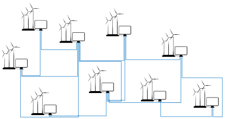
Figure 1: Communication network topology for nine MPs

6.1 Verification of the Distributed Modified IGMM

For the chosen nine MPs, the distributed modified IGMM generates nine groups of updated results. We choose the 1st group, i.e., the updated result of the 1st MP, for illustration. Thus, we must first verify the rationality of this choice.

Note that each MP does not own the complete updated parameter set of the joint PD, i.e., $\bm{\mu}_{j}$, $w_{j}$ and $\bm{\Sigma}_{j}$ for $j=1,...,J$, but only owns the updated $\mu_{j,x_{m}}$, $\mu_{j,y_{m}}$, $w_{j}$ and $\bm{\Sigma}_{j}$ for $j=1,...,J$. To illustrate the consensus effect of the distributed modified IGMM, we collect each MP’s updated private mean value $\mu_{j,x_{m}}$ and $\mu_{j,y_{m}}$ to form a complete $\bm{\mu}_{j}$. Combining this $\bm{\mu}_{j}$ with each MP’s $w_{j}$ and $\bm{\Sigma}_{j}$, we obtain nine complete updated parameter sets of the joint PD, which are essentially nine updated joint PDs. Then, we derive the marginal PD of the 1st dimension from each updated joint PD to illustrate the differences among the updated results of the MPs. The 9 marginal PDs are shown in Fig. 2 in the form of the PD function (PDF). As shown, the PDFs built by different MPs are essentially the same. To quantify the differences, we calculate the Jensen–Shannon divergence between the complete updated joint PD built by the 1st MP and those by the other MPs and provide the results in Table I. All the Jensen–Shannon divergences are lower than $9.83\times 10^{-12}$, which is an extremely low value relative to 1. Thus, the differences between the updated results of each MP are indeed small. Therefore, the consensus effect of the distributed modified IGMM is verified, and using the results of the 1st MP as a representative is also reasonable.

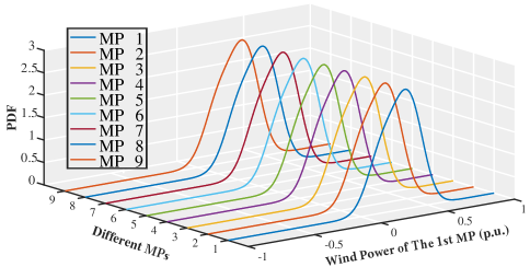
Figure 2: The marginal PDF of the first dimension built by different MPs

TABLE I: The Jensen–Shannon Divergence Between the 1st MP and Other MPs

MP	$1$	$2$	$3$	$4$	$5$	$6$	$7$	$8$	$9$
Divergence ($\times 10^{-12}$)	0	1.28	9.83	2.00	4.76	5.02	5.03	3.80	6.37

To verify the effectiveness and correctness of the distributed modified IGMM, we utilize the entire dataset, i.e., the combined historical and new dataset, as the training set, and we use the centralized EM algorithm for training. This training result is considered the final benchmark for the incremental update. Then, we use the proposed distributed modified IGMM to update the old PD, which is built using only the historical dataset. Because the new dataset has 960 pieces of new data, the distributed modified IGMM needs to be performed 960 times for the final complete update. For a clear illustration, we derive the marginal PD of the 1st dimension from the updated results. The marginal PDFs built by the centralized EM algorithm and distributed modified IGMM are shown in Fig. 3. The benchmark is the result obtained by the centralized EM algorithm with the entire dataset. ‘D-U’ represents the result of the distributed modified IGMM after 960 updates, and ‘D-N’ represents the result of the old PD built by the historical dataset. The legend ‘D-U$n$’ denotes the update result of the distributed modified IGMM after $n\times 96$ updates. From this illustration, we can draw two conclusions: (1) the effectiveness of the distributed modified IGMM is verified because as the number of updates increases, the updated PDF curves built by the distributed modified IGMM are gradually moving away from the ‘D-N’ curve and approaching the benchmark in the direction of the black arrow. (2) The correctness of the distributed modified IGMM is verified because the curve ‘D-U’ and the benchmark are coincident.

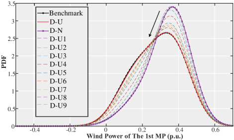
Figure 3: The marginal PDF of the first dimension

To verify the efficiency of the distributed modified IGMM, we compare the computational times of the centralized EM algorithm and the proposed distributed modified IGMM for each update. Note that the centralized EM algorithm has to reconstruct the training dataset whenever new data are generated and train this set to obtain the updated PD result. Besides, the calculation time of the proposed distributed modified IGMM refers to the time consumed by one MP, while the calculation time of the centralized EM algorithm refers to the time consumed by a data center. Although there are 960 updates, for a clear demonstration, we only illustrate the computational time for the 6th, 12th, 18th, ……, and 960th updates. The details are presented in Fig. 4, which shows that the computational time of the distributed modified IGMM is much less than the computational time of the centralized EM algorithm. Meanwhile, as the size of the historical dataset increases, the computational time of the centralized EM algorithm also increases, but that of the proposed distributed modified IGMM is stable because the calculation burden of a piece of new data is always the same. Further comparisons of the computational time for all 960 updates are given in Table II. The results show that the proposed distributed modified IGMM is considerably more efficient than the centralized EM algorithm.

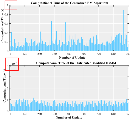
Figure 4: The computational time for each update

TABLE II: Computational Time comparison

	Centralized EM	distributed modified IGMM	Reduction
Maximum	$1344\times 10^{-3}$s	$1.22\times 10^{-3}$s	11006%
Minimum	$69\times 10^{-3}$s	$0.33\times 10^{-3}$s	20809%
Mean	$195\times 10^{-3}$s	$0.67\times 10^{-3}$s	29004%

Note that even though the computational times of the EM algorithm are much higher than those of the proposed algorithm, the computational times are still lower than 1 second. This is because the dataset for testing consists of only 1920 pieces of observations. When the dataset grows over time with more integration of DWGs, the computational cost of the centralized EM algorithm will continue to increase quickly, but the computational cost of the proposed algorithm will still be much less than that of the EM algorithm and stable. To make a further comparison using a large training dataset, we choose 27 sites in Ohio from the Wind Dataset published by the National Renewable Energy Laboratory. The old dataset consists of 15,000 pieces of observation, while the new dataset consists of 10,000 pieces of observation. The computational times for the 7,500-th, 8,000th, …, 10,000th updates are shown in Fig. 5.

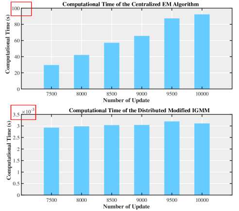
Figure 5: The computational time for each update using a large dataset

From this illustration, we can draw these conclusions:

• When a dataset grows, the computational time of the centralized EM algorithm increases sharply, e.g., the computational time for the 10,000th update approaches 100 seconds. Therefore, using the centralized EM algorithm for updating may indeed be a problem.

• When the number of DWGs increases from 9 to 27, the computational time of the proposed algorithm increases slightly, i.e., from $1\times 10^{-3}s$ to $3\times 10^{-3}s$. Compared to the computational time of the 10,000th update using the centralized EM algorithm, the efficiency is improved by $2.9709\times 10^{6}\%$. Therefore, the improvement made by the proposed algorithm is scalable when the dimension of the update problem increases.

• When the number of updates increases from 7,500 to 10,000, the computational times of the proposed algorithm remain low and stable. Compared to the centralized EM algorithm, the improvements vary from $1.0097\times 10^{6}\%$ to $2.9708\times 10^{6}\%$. Therefore, the improvement made by the proposed algorithm is scalable when the number of updates increases.

It should be emphasized that, due to the tiny computational cost of the distributed modified IGMM, this algorithm is sufficient for the needs of real time update.

6.2 Verification of the Distributed Incremental Update Scheme

Note that, the following case studies still use the small dataset consisting of 960 old observations and 960 new observations owned by nine MPs.

To verify the effectiveness of the distributed incremental update scheme, we first use the entire dataset to build the empirical distributions under a given wind power forecast of correlated MPs. Then, we use the EM algorithm to build the latest marginal PD of each MP’s WPFE based on the entire dataset without considering the correlation between DWGs. Finally, we use the proposed scheme to update each MP’s conditional PD until the conditional PDs are the latest. The conditional PDs are shown in Fig. 6 in the form of PDFs. The conditional PDs of the first four MPs are shown. The updated conditional PDs built by the proposed scheme are more concentrated than the marginal PDs, making the characterization of the uncertainty more precise. This will greatly reduce the operation cost for each MP, e.g., the cost of reserve scheduling. Let’s take the fourth subfigure in Fig. 6 for illustration. If the 4-th MP uses the updated marginal PDF to schedule reserves, a 0.6 (p.u.) down reserve and a 0.1 (p.u.) up reserve are required. However, if the conditional PDF is used, only a 0.13 (p.u.) down reserve and a 0.1 (p.u.) up reserve are required. Therefore, when using the updated conditional PDF for reserve scheduling, a huge cost of reserve will be saved. In addition, the updated conditional PDFs also match the empirical distributions well.

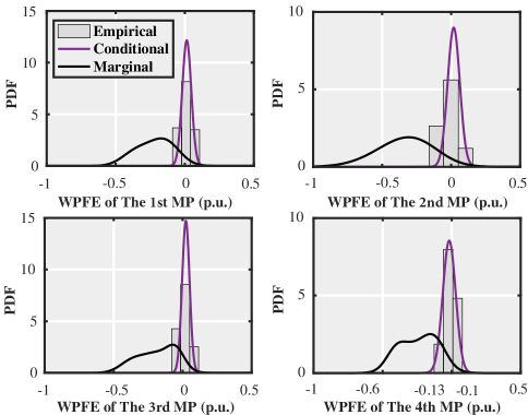
Figure 6: comparison of PDFs

To verify the correctness of this scheme, we build each MP’s conditional PD in different ways. First, we use a centralized EM algorithm to build the latest joint PD using the entire dataset and then derive each MP’s conditional PD by collecting their wind power forecast data. These results are also considered as the benchmark and represented by the legend ‘C-S’. Second, we use the centralized EM algorithm to build the old PD using the historical dataset and then to derive each MP’s conditional PD in a centralized manner. These results are represented by the legend ‘C-N’. Finally, we use the proposed scheme to update each MP’s conditional PD until the conditional PDs are the latest. We use the legend ‘D-U’ to represent these results. The conditional PDs of the first four MPs built by the three approaches are demonstrated in Fig. 7 in the form of CDF.

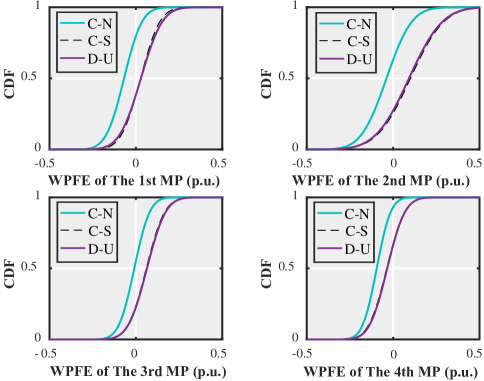
Figure 7: comparison of CDFs

TABLE III: RSE comparison

	1st MP	2nd MP	3rd MP	4th MP
C-N	$6.68\%$	$9.74\%$	$3.78\%$	$2.83\%$
D-U	$0.040\%$	$0.038\%$	$0.013\%$	$0.009\%$

As shown, curve ‘D-U’ is coincident with the benchmark curve ‘C-S’, while curve ‘C-N’ differs greatly from the benchmark. The difference between the benchmark with curve ‘C-N’ and the difference between the benchmark and curve ‘D-U’ are measured by the relative standard error (RSE) and provided in Table III. Based on these illustrations, we know that the conditional PD updated by the scheme is correct because the RSE value between curve ‘D-U’ and the benchmark is lower than $4\times 10^{-4}$, and curve ‘D-U’ fits the benchmark.

7. Conclusion

In this paper, we focus on MPs who own DWGs in a distribution network. To make them perform better in the local market considering the wind power uncertainty, we propose a distributed incremental update scheme to update each MP’s conditional PD of the WPFE in a fully distributed manner with the consideration of the DWGs’ correlation. This scheme consists of two original algorithms. One is a distributed modified IGMM for updating the parameters of the joint PD. Another one is a distributed derivation algorithm for deriving conditional PDs. This scheme can make each MP’s conditional PD of the WPFE stay up to date with an extremely low and stable update cost, regardless of how much the historical dataset increases. In addition, this scheme is fully distributed without any data center or coordinator. Moreover, the conditional PD of the WPFE updated by the scheme is more concentrated and precise than the marginal PD, as the correlation among DWGs is taken into account.

Acknowledgements

This work is supported in part by the Joint Funds of the National Natural Science Foundation of China under Grant U1766206.

References

- [1] T. Morstyn, N. Farrell, S. J. Darby, and M. D. McCulloch, “Using peer-to-peer energy-trading platforms to incentivize prosumers to form federated power plants,” Nature Energy, vol. 3, no. 2, pp. 94–101, 2018.
- [2] A. Lüth, J. M. Zepter, P. C. del Granado, and R. Egging, “Local electricity market designs for peer-to-peer trading: The role of battery flexibility,” Appl. Energy., vol. 229, pp. 1233 – 1243, 2018. [Online]. Available: http://www.sciencedirect.com/science/article/pii/S0306261918311590
- [3] Y. Liu, K. Zuo, X. A. Liu, J. Liu, and J. M. Kennedy, “Dynamic pricing for decentralized energy trading in micro-grids,” Appl. Energy., vol. 228, pp. 689 – 699, 2018. [Online]. Available: http://www.sciencedirect.com/science/article/pii/S0306261918309930
- [4] H. Yi, M. H. Hajiesmaili, Y. Zhang, M. Chen, and X. Lin, “Impact of the uncertainty of distributed renewable generation on deregulated electricity supply chain,” IEEE Trans. Smart Grid., vol. 9, no. 6, pp. 6183–6193, Nov 2018.
- [5] Z. Zhang, Y. Sun, D. W. Gao, J. Lin, and L. Cheng, “A versatile probability distribution model for wind power forecast errors and its application in economic dispatch,” IEEE Trans. Power Syst., vol. 28, no. 3, pp. 3114–3125, Aug 2013.
- [6] J. Wu, B. Zhang, H. Li, Z. Li, Y. Chen, and X. Miao, “Statistical distribution for wind power forecast error and its application to determine optimal size of energy storage system,” INT J ELEC POWER., vol. 55, pp. 100 – 107, 2014. [Online]. Available: http://www.sciencedirect.com/science/article/pii/S0142061513003761
- [7] A. Fabbri, T. G. S. Roman, J. R. Abbad, and V. H. M. Quezada, “Assessment of the cost associated with wind generation prediction errors in a liberalized electricity market,” IEEE Trans. Power Syst., vol. 20, no. 3, pp. 1440–1446, Aug 2005.
- [8] L. Exizidis, S. J. Kazempour, P. Pinson, Z. de Greve, and F. Vallée, “Sharing wind power forecasts in electricity markets: A numerical analysis,” Appl. Energy., vol. 176, pp. 65 – 73, 2016. [Online]. Available: http://www.sciencedirect.com/science/article/pii/S0306261916306468
- [9] Z. W. Wang, C. Shen, and F. Liu, “Probabilistic analysis of small signal stability for power systems with high penetration of wind generation,” IEEE Trans. Sustain. Energy., vol. 7, no. 3, pp. 1182–1193, July 2016.
- [10] Z. Wang, C. Shen, F. Liu, X. Wu, C. Liu, and F. Gao, “Chance-constrained economic dispatch with non-gaussian correlated wind power uncertainty,” IEEE Trans. Power Syst., vol. 32, no. 6, pp. 4880–4893, Nov 2017.
- [11] Z. Wang, C. Shen, and F. Liu, “A conditional model of wind power forecast errors and its application in scenario generation,” Appl. Energy., vol. 212, pp. 771–785, 2018.
- [12] F. Bouffard and F. D. Galiana, “Stochastic security for operations planning with significant wind power generation,” IEEE Trans. Power Syst., vol. 23, no. 2, pp. 306–316, May 2008.
- [13] B. Hodge and M. Milligan, “Wind power forecasting error distributions over multiple timescales,” in Proc. IEEE PES General Meeting, July 2011, pp. 1–8.
- [14] Y. Wu, P. Su, and J. Hong, “An overview of wind power probabilistic forecasts,” in Proc. IEEE PES Asia-Pacific Power and Energy Engineering Conference (APPEEC), Oct 2016, pp. 429–433.
- [15] K. Bruninx and E. Delarue, “A statistical description of the error on wind power forecasts for probabilistic reserve sizing,” IEEE Trans. Sustain. Energy., vol. 5, no. 3, pp. 995–1002, July 2014.
- [16] S. Tewari, C. J. Geyer, and N. Mohan, “A statistical model for wind power forecast error and its application to the estimation of penalties in liberalized markets,” IEEE Trans. Power Syst., vol. 26, no. 4, pp. 2031–2039, Nov 2011.
- [17] N. Menemenlis, M. Huneault, and A. Robitaille, “Computation of dynamic operating balancing reserve for wind power integration for the time-horizon 1–48 hours,” IEEE Trans. Sustain. Energy., vol. 3, no. 4, pp. 692–702, Oct 2012.
- [18] W. Lin, J. Wen, S. Cheng, and W.-J. Lee, “An investigation on the active power variations of wind farms,” in Proc. IEEE Industry Applications Society Annual Meeting, Oct 2011, pp. 1–8.
- [19] Z. Zhang, Y. Sun, J. Lin, L. Cheng, and G. Li, “Versatile distribution of wind power output for a given forecast value,” in Proc. IEEE PES General Meeting, July 2012, pp. 1–7.
- [20] C. Tang, J. Xu, Y. Sun, J. Liu, X. Li, D. Ke, J. Yang, and X. Peng, “A versatile mixture distribution and its application in economic dispatch with multiple wind farms,” IEEE Trans. Sustain. Energy., vol. 8, no. 4, pp. 1747–1762, Oct 2017.
- [21] R. Singh, B. C. Pal, and R. A. Jabr, “Statistical representation of distribution system loads using gaussian mixture model,” IEEE Trans. Power Syst., vol. 25, no. 1, pp. 29–37, Feb 2010.
- [22] Z. Wang, C. Shen, Y. Xu, F. Liu, X. Wu, and C. Liu, “Risk-limiting load restoration for resilience enhancement with intermittent energy resources,” IEEE Trans. Smart Grid., pp. 1–1, 2018.
- [23] M. Nijhuis, M. Gibescu, and S. Cobben, “Gaussian mixture based probabilistic load flow for lv-network planning,” IEEE Trans. Power Syst., vol. 32, no. 4, pp. 2878–2886, July 2017.
- [24] M. Jia, C. Shen, and Z. Wang, “A distributed probabilistic modeling algorithm for the aggregated power forecast error of multiple newly built wind farms,” IEEE Trans. Sustain. Energy., pp. 1–1, 2018.
- [25] M. Song and H. Wang, “Highly efficient incremental estimation of gaussian mixture models for online data stream clustering,” in Proc. Intelligent Computing: Theory and Applications III, vol. 5803, 2005, pp. 174–184.
- [26] A. Declercq and J. H. Piater, “Online learning of gaussian mixture models-a two-level approach.” in VISAPP (I), 2008, pp. 605–611.
- [27] C. Chen, D. Mu, H. Zhang, and W. Hu, “Incremental learning of gaussian mixture model: A top-down algorithm,” Journal of Computational Information Systems, vol. 9, no. 17, pp. 6971–6980, 2013.
- [28] A. Bouchachia and C. Vanaret, “Incremental learning based on growing gaussian mixture models,” in Proc. 10th IEEE International Conference on Machine Learning and Applications and Workshops, vol. 2, 2011, pp. 47–52.
- [29] C. Stauffer and W. E. L. Grimson, “Adaptive background mixture models for real-time tracking,” in Proc. 1999 IEEE Computer Society Conference on Computer Vision and Pattern Recognition (Cat. No PR00149), vol. 2, June 1999, pp. 246–252 Vol. 2.
- [30] A. Ribes, J. C. Bueno, Y. Demiris, and R. L. de Mántaras, “Context-gmm: Incremental learning of sparse priors for gaussian mixture regression,” in Proc. IEEE International Conference on Robotics and Biomimetics (ROBIO), Dec 2012, pp. 1446–1451.
- [31] R. C. Pinto and P. M. Engel, “A fast incremental gaussian mixture model,” PloS one, vol. 10, no. 10, 2015.
- [32] R. Pinto and P. Engel, “Scalable and incremental learning of gaussian mixture models,” arXiv preprint arXiv:1701.03940, 2017.
- [33] M. Jia and C. Shen, “Privacy-preserving distributed joint probability modeling for spatial-correlated wind farms,” arXiv preprint arXiv:1812.09247, 2018.
- [34] R. Olfati-Saber, J. A. Fax, and R. M. Murray, “Consensus and cooperation in networked multi-agent systems,” Proc. of the IEEE, vol. 95, no. 1, pp. 215–233, Jan 2007.