On the monotonicity and discrete maximum principle of the finite difference implementation of $C^{0}$-$Q^{2}$ finite element method

Abstract

We show that the fourth order accurate finite difference implementation of continuous finite element method with tensor product of quadratic polynomial basis is monotone thus satisfies the discrete maximum principle for solving a scalar variable coefficient equation $-\nabla\cdot(a\nabla u)+cu=f$ under a suitable mesh constraint.

65N30, 65N06, 65N12

1 Introduction

1.1 Monotonicity and discrete maximum principle

Consider a Poisson equation with variable coefficients and Dirichlet boundary conditions on a two dimensional rectangular domain $\Omega=(0,1)\times(0,1)$:

(1) $$\begin{split}\mathcal{L}u\equiv-\nabla\cdot(a\nabla u)+cu=0&\quad\mbox{on}\quad\Omega,\\ u=g&\quad\mbox{on}\quad\partial\Omega,\end{split}$$

where $a(x,y),c(x,y)\in C^{0}(\bar{\Omega})$ with $0<a_{\min}\leq a(x,y)\leq a_{\max}$ and $c(x,y)\geq 0$. For a smooth function $u\in C^{2}(\Omega)\cap C(\bar{\Omega})$, maximum principle holds [12]: $\mathcal{L}u\leq 0\,\,\mbox{in}\,\,\Omega\Longrightarrow\max_{\bar{\Omega}}u\leq\max\left\{0,\max_{\partial\Omega}u\right\},$ and in particular,

(2) $$\mathcal{L}u=0\,\,\mbox{in}\,\,\Omega\Longrightarrow|u(x,y)|\leq\max\limits_{\partial\Omega}|u|,\quad\forall(x,y)\in\Omega.$$

For various purposes, it is desired to have numerical schemes to satisfy (2) in the discrete sense. A linear approximation to $\mathcal{L}$ can be represented as a matrix $L_{h}$. The matrix $L_{h}$ is called monotone if its inverse has nonnegative entries, i.e., $L_{h}^{-1}\geq 0$. All matrix inequalities in this paper are entrywise inequalities. One sufficient condition for the discrete maximum principle is the monotonicity of the scheme, which was also used to prove convergence of numerical schemes, e.g., [4, 10, 1, 13].

In this paper, we will discuss the monotonicity and discrete maximum principle of the simplest finite difference implementation of the continuous finite element method with $Q^{2}$ basis (i.e., tensor product of quadratic polynomial) for (1), which is a fourth order accurate scheme [20].

1.2 Second accurate schemes and M-matrices

The second order centered difference $u^{\prime\prime}\approx\frac{u_{i-1}-2u_{i}+u_{i+1}}{\Delta x^{2}}$ for solving $-u^{\prime\prime}(x)=f(x),u(0)=u(1)=0$ results in a tridiagonal $(-1,2,-1)$ matrix, which is an M-matrix. Nonsingular M-matrices are inverse-positive matrices and it is the most convenient tool for constructing inverse-positive matrices. There are many equivalent definitions or characterizations of M-matrices, see [24]. One convenient characterization of nonsingular M-matrices are nonsingular matrices with nonpositive off-diagonal entries and positive diagonal entries, and all row sums are non-negative with at least one row sum is positive.

The continuous finite element method with piecewise linear basis forms an M-matrix for the variable coefficient problem (1) on triangular meshes under reasonable mesh constraints [33]. The M-matrix structure in linear finite element method also holds for a nonlinear elliptic equation [15]. For solving $-\Delta u=f$ on regular triangular meshes, linear finite element method reduces to the 5-point discrete Laplacian. Linear finite element method or the 5-point discrete Laplacian is the most popular method in the literature for constructing schemes satisfying a discrete maximum principle and bound-preserving properties.

Almost all high order accurate schemes result in positive off-diagonal entries in $L_{h}$ for solving $-\Delta u=f$ thus $L_{h}$ is no longer an M-matrix. The only known exceptions are the fourth order accurate 9-point discrete Laplacian and the fourth order accurate compact finite difference scheme.

1.3 Existing high order accurate monotone methods for two-dimensional Laplacian

There are at least three kinds of high order accurate schemes which have been proven to satisfy $L^{-1}_{h}\geq 0$ for the Laplacian operator $\mathcal{L}u=-\Delta u$:

1. Both the fourth order accurate 9-point discrete Laplacian scheme [4, 6] and the fourth order accurate compact finite difference scheme [18, 19] for $-\Delta u=f$ can be written as $S\mathbf{u}=W\mathbf{f}$ with $S$ being an M-matrix and $W\geq 0$, thus $L_{h}^{-1}=S^{-1}M\geq 0$.

2. In [5, 7], Bramble and Hubbard constructed a fourth order accurate finite difference discrete Laplacian operator for which $L_{h}$ is not an M-matrix but monotonicity $L^{-1}_{h}\geq 0$ is ensured through an M-matrix factorization $L_{h}=M_{1}M_{2}$, i.e., $L_{h}$ is a product of two M-matrices.

3. Finite element method with quadratic polynomial (P2 FEM) basis on a regular triangular mesh can be implemented as a finite difference scheme defined at vertices and edge centers of triangles [31]. The error estimate of P2 FEM is third order in $L^{2}$-norm. The stiffness matrix is not an M-matrix but its monotonicity was proven in [22].

For discrete maximum principle to hold in P2 FEM on a generic triangular mesh, it was proven in [14] that it is necessary and sufficient to require a very strong mesh constraint, which essentially gives either regular triangulation or equilateral triangulation. Thus discrete maximum principle holds in P2 FEM on a regular triangulation or an equilateral triangulation. For finite element method with cubic and higher order polynomials on regular triangular meshes, it was shown that discrete maximum principle fails in [28].

1.4 Other known results regarding discrete maximum principle

For one-dimensional Laplacian, discrete maximum principle was proven for arbitrarily high order finite element method using discrete Green’s function in [30]. The discrete Green’s function was also used to analyze P1 FEM in two dimensions [11]. Discontinuous coefficients were considered and a nonlinear scheme was constructed in [21]. Piecewise constant coefficient in one dimension was considered in [29]. A numerical study for high order FEM with very accurate Gauss quadrature in two dimensions showed that DMP was violated on non-uniform unstructured meshes for variable coefficients in [23]. A more general operator $\nabla(\mathbf{a}\nabla u)$ with matrix coefficients $\mathbf{a}$ was considered for linear FEM in [16]. See [17] for an anisotropic computational example.

1.5 Existing inverse-positive approaches when $L_{h}$ is not an M-matrix

In this paper, we will focus on the finite difference implementation of continuous finite element method with $Q^{2}$ basis (Q2 FEM), which will be reviewed in Section 2. The matrix $L_{h}$ in such a scheme is not an M-matrix due to its off-diagonal positive entries. There are at least three methods to study whether $L^{-1}_{h}\geq 0$ holds when M-matrix structure is lost:

1. An M-matrix factorization of the form $L_{h}=M_{1}M_{2}$ was shown in [7] and [2]. In Appendix A, we will demonstrate an M-matrix factorization for the finite difference implementation of $Q^{2}$ FEM solving $-\Delta u=f$.

2. Perturbation of M-matrices by positive offdiagonal entries without losing monotonicity was discussed in [3].

3. In [22], Lorenz proposed a sufficient condition for ensuring $L_{h}=M_{1}M_{2}$. Lorenz’s condition will be reviewed in Section 3.3.

The main result of this paper is to prove that $L_{h}^{-1}\geq 0$ and a discrete maximum principle holds under some mesh constraint in the fourth order accurate finite difference implementation of $Q^{2}$ FEM solving (1) by verifying the Lorenz’s condition.

1.6 Extensions to discrete maximum principle for parabolic equations

Classical solutions to the parabolic equation $u_{t}=\nabla\cdot(a\nabla u)$ satisfy a maximum principle [12]. With suitable boundary conditions and initial value $u(x,y,0)$ such as periodic or homogeneous Dirichlet boundary conditions and $\min\limits_{\Omega}u(x,y,0)=0$, the solution to the initial value problem satisfies the following maximum principle:

(3) $$\min_{(x,y)}u(x,y,0)\leq u(x,y,t)\leq\max_{(x,y)}u(x,y,0).$$

Now consider solving $u_{t}=\nabla\cdot(a\nabla u)$ with backward Euler time discretization, then $U^{n+1}$ satisfies an elliptic equation of the form (1):

(4) $$-\nabla\cdot(a\nabla U^{n+1})+\frac{1}{\Delta t}U^{n+1}=\frac{1}{\Delta t}U^{n}.$$

If $S_{h}$ denotes spatial discretization for $-\nabla\cdot(a\nabla u)$, then the numerical scheme can be written as $U^{n+1}=(I+\Delta tS_{h})^{-1}U^{n}$. Let $\mathbf{1}=\begin{bmatrix}1&1&\cdots&1\end{bmatrix}^{T}$, then for suitable boundary conditions usually we have $S_{h}\mathbf{1}=\mathbf{0}$ since $S_{h}$ approximates a differential operator. So we have $(I+\Delta tS_{h})\mathbf{1}=\mathbf{1}$ thus $(I+\Delta tS_{h})^{-1}\mathbf{1}=\mathbf{1}$. If we further have the monotonicity $(I+\Delta tS_{h})^{-1}\geq 0$, then each row of the $(I+\Delta tS_{h})^{-1}$ has nonnegative entries and sums to one, thus the discrete maximum principle holds $\min_{j}U_{j}^{n}\leq U^{n+1}_{j}\leq\max_{j}U_{j}^{n}$, which is a desired and useful property in many applications. For instance, second order centered difference or P1 finite element method has been used to construct schemes satisfying the discrete maximum principle in solving phase field equations [27, 26, 32]. In the rest of the paper, we will only focus on discussing the equation (1), even though all discussions can be extended to solving the parabolic equation with backward Euler time discretization.

1.7 Contributions and organization of the paper

To the best of our knowledge, this is the first time that a high order accurate scheme under suitable mesh constraints is proven to be monotone in the sense $L_{h}^{-1}\geq 0$ for solving a variable coefficient $a(\mathbf{x})$ in (1) in two dimensions. For simplicity, we only discuss an uniform mesh in this paper, even though the main results can be extended to non-uniform meshes. However, an additional mesh constraint is expected for discrete maximum principle to hold. See such a mesh constraint of non-uniform meshes for Q1 FEM in [8] and P2 FEM for one-dimensional problem in [30].

This paper is organized as follows. In Section 2, we describe the fourth order accurate finite difference implementation of $C^{0}$-$Q^{2}$ finite element method. In Section 3, we review the sufficient conditions to ensure monotonicity and discrete maximum principle. In Section 4, we prove that the fourth order accurate finite difference implementation of $C^{0}$-$Q^{2}$ finite element method is monotone under some mesh constraints. Numerical tests are given in Section 5. Concluding remarks are given in Section 6.

2 Finite difference implementation of $C^{0}$-$Q^{2}$ finite element method

Consider solving the following elliptic equation on $\Omega=(0,1)\times(0,1)$ with Dirichlet boundary conditions:

(5) $$\begin{split}\mathcal{L}u\equiv-\nabla\cdot(a\nabla u)+cu=f&\quad\mbox{on}\quad\Omega,\\ u=g&\quad\mbox{on}\quad\partial\Omega.\end{split}$$

Assume there is a function $\bar{g}\in H^{1}(\Omega)$ as an extension of $g$ so that $\bar{g}|_{\partial\Omega}=g$. The variational form of (1) is to find $\tilde{u}=u-\bar{g}\in H_{0}^{1}(\Omega)$ satisfying

(6) $$\mathcal{A}(\tilde{u},v)=(f,v)-\mathcal{A}(\bar{g},v),\quad\forall v\in H_{0}^{1}(\Omega),$$

where $\mathcal{A}(u,v)=\iint_{\Omega}a\nabla u\cdot\nabla vdxdy+\iint_{\Omega}cuvdxdy$, $(f,v)=\iint_{\Omega}fvdxdy.$

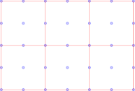
(a) The quadrature points and a FEM mesh

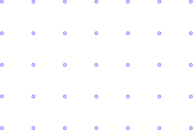
(b) The corresponding finite difference grid

Figure 1: An illustration of $Q^{2}$ element and the $3\times 3$ Gauss-Lobatto quadrature.

Let $h$ be the mesh size of the rectangular mesh and $V_{0}^{h}\subseteq H^{1}_{0}(\Omega)$ be the continuous finite element space consisting of piecewise $Q^{2}$ polynomials (i.e., tensor product of piecewise quadratic polynomials), then the most convenient implementation of $C^{0}$-$Q^{2}$ finite element method is to use $3\times 3$ Gauss-Lobatto quadrature rule for all the integrals, see Figure 1. Such a numerical scheme can be defined as: find $u_{h}\in V_{0}^{h}$ satisfying

(7) $$\mathcal{A}_{h}(u_{h},v_{h})=\langle f,v_{h}\rangle_{h}-\mathcal{A}_{h}(g_{I},v_{h}),\quad\forall v_{h}\in V_{0}^{h},$$

where $\mathcal{A}_{h}(u_{h},v_{h})$ and $\langle f,v_{h}\rangle_{h}$ denote using tensor product of $3$-point Gauss Lobatto quadrature for integrals $\mathcal{A}(u_{h},v_{h})$ and $(f,v_{h})$ respectively, and $g_{I}$ is the piecewise $Q^{2}$ Lagrangian interpolation polynomial at the $3\times 3$ quadrature points shown in Figure 1 of the following function:

$$g(x,y)=\begin{cases}0,&\mbox{if}\quad(x,y)\in(0,1)\times(0,1),\\ g(x,y),&\mbox{if}\quad(x,y)\in\partial\Omega.\\ \end{cases}$$

Then $\bar{u}_{h}=u_{h}+g_{I}$ is the numerical solution for the problem (5). We emphasize that (7) is not a straightforward approximation to (6) since $\bar{g}$ is never used. It was proven in [20] that the scheme (7) is fourth order accurate if coefficients and exact solutions are smooth. Notice that $\bar{u}_{h}$ satisfies:

(8) $$\mathcal{A}_{h}(\bar{u}_{h},v_{h})=\langle f,v_{h}\rangle_{h},\quad\forall v_{h}\in V_{0}^{h}.$$

See [20] for the detailed finite difference implementation and proof of fourth order accuracy for the scheme (7).

2.1 One-dimensional case

Now consider the one-dimensional Dirichlet boundary value problem:

$$-(au^{\prime})^{\prime}+cu= f\textrm{ on }(0,1),$$

$$u(0)=\sigma_{0},\quad u(1)=\sigma_{1}.$$

Consider a uniform mesh $x_{i}=ih$, $i=0,1,\dots,n+1$, $h=\frac{1}{n+1}$. Assume $n$ is odd and let $M=\frac{n+1}{2}$. Define intervals $I_{k}=[x_{2k},x_{2k+2}]$ for $k=0,\dots,M-1$ as a finite element mesh for $P^{2}$ basis. Define

$$V^{h}=\{v\in C^{0}([0,1]):v\in P^{2}(I_{k}),k=0,\dots,M-1\}.$$

Let $\{\phi_{i}\}_{i=0}^{n+1}\subset V^{h}$ be a basis for $V^{h}$ so that $\phi_{i}(x_{j})=\delta_{ij},\,i,j=0,1,\dots,n+1$. Let $u_{i}=u_{h}(x_{i})$, $u_{0}=\sigma_{0}$ and $u_{n+1}=\sigma_{1}$, then $u_{h},\bar{u}_{h}\in V^{h}$ can be represented as

$$u_{h}(x)=\sum_{i=1}^{n}u_{i}\phi_{i}(x),\quad\bar{u}_{h}(x)=\sum_{i=0}^{n+1}u_{i}\phi_{i}(x).$$

Let $f_{j}=f(x_{j})$, then (8) becomes

$$\langle au_{h}^{\prime},\phi_{i}^{\prime}\rangle_{h}+\langle cu_{h},\phi_{i}\rangle_{h}=\langle f,\phi_{i}\rangle_{h},\quad i=1,\dots,n;u_{0}=\sigma_{0},u_{n+1}=\sigma_{1},$$

which are

$$\sum_{j=0}^{n+1}u_{j}\left(\langle a\phi_{j}^{\prime},\phi_{i}^{\prime}\rangle_{h}+\langle c\phi_{j},\phi_{i}\rangle_{h}\right)=\sum_{j=0}^{n+1}f_{j}\langle\phi_{j},\phi_{i}\rangle_{h},\quad i=1,\dots,n;u_{0}=\sigma_{0},u_{n+1}=\sigma_{1}.$$

The matrix form is $S\bar{\mathbf{u}}=M\bar{\mathbf{f}}$ where

$$\bar{\mathbf{u}}=\begin{bmatrix}u_{0}&u_{1}&u_{2}\cdots&u_{n}&u_{n+1}\end{bmatrix}^{T},\quad\bar{\mathbf{f}}=\begin{bmatrix}\sigma_{0}&f_{1}&f_{2}\cdots&f_{n}&\sigma_{1}\end{bmatrix}^{T}.$$

The scheme can be written as $\mathcal{L}_{h}(\bar{\mathbf{u}})=\bar{\mathbf{f}}$. The linear operator $\mathcal{L}_{h}$ has the matrix representation $L_{h}=M^{-1}S$.

For the Laplacian $\mathcal{L}u=-u^{\prime\prime}$, we have

(9a) $$\mathcal{L}_{h}(\bar{\mathbf{u}})_{0} =u_{0}=\sigma_{0},\quad\mathcal{L}_{h}(\bar{\mathbf{u}})_{n+1}=u_{n+1}=\sigma_{1},$$

(9b) $$\mathcal{L}_{h}(\bar{\mathbf{u}})_{i} =\frac{-u_{i-1}+2u_{i}-u_{i+1}}{h^{2}}=f_{i},\quad\mbox{if $i$ is odd, i.e., $x_{i}$ is a cell center},$$

(9c) $$\mathcal{L}_{h}(\bar{\mathbf{u}})_{i} =\frac{u_{i-2}-8u_{i-1}+14u_{i}-8u_{i+1}+u_{i+2}}{4h^{2}}=f_{i},\quad\mbox{if $i$ is even, i.e., $x_{i}$ is a cell end}.$$

For the variable coefficient operator $\mathcal{L}u=-(au^{\prime})^{\prime}+cu$, we have

(10a) $$\mathcal{L}_{h}(\bar{\mathbf{u}})_{0}=u_{0}=\sigma_{0},\quad\mathcal{L}_{h}(\bar{\mathbf{u}})_{n+1}=u_{n+1}=\sigma_{1},$$

and if $$x_{i}$$ is a cell center, we have

(10b) $$\mathcal{L}_{h}(\bar{\mathbf{u}})_{i}=\frac{-(3a_{i-1}+a_{i+1})u_{i-1}+4(a_{i-1}+a_{i+1})u_{i}-(a_{i-1}+3a_{i+1})u_{i+1}}{4h^{2}}+c_{i}u_{i}=f_{i};$$

and if $$x_{i}$$ is a cell end, then

$$\mathcal{L}_{h}(\bar{\mathbf{u}})_{i}=\frac{(3a_{i-2}-4a_{i-1}+3a_{i})u_{i-2}-(4a_{i-2}+12a_{i})u_{i-1}+(a_{i-2}+4a_{i-1}+18a_{i}+4a_{i+1}+a_{i+2})u_{i}}{8h^{2}}$$

(10c) $$+\frac{-(12a_{i}+4a_{i+2})u_{i+1}+(3a_{i+2}-4a_{i+1}+3a_{i})u_{i+2}}{8h^{2}}+c_{i}u_{i}=f_{i}.$$

2.2 Two-dimensional case

Consider a uniform grid $(x_{i},y_{j})$ for a rectangular domain $[0,1]\times[0,1]$ where $x_{i}=ih$, $i=0,1,\dots,n+1$ and $y_{j}=jh$, $j=0,1,\dots,n+1$, $h=\frac{1}{n+1}$, where $n$ must be odd. Let $u_{ij}$ denote the numerical solution at $(x_{i},y_{j})$. Let $\mathbf{u}$ denote an abstract vector consisting of $u_{ij}$ for $i,j=1,2,\cdots,n$. Let $\bar{\mathbf{u}}$ denote an abstract vector consisting of $u_{ij}$ for $i,j=0,1,2,\cdots,n,n+1$. Let $\bar{\mathbf{f}}$ denote an abstract vector consisting of $f_{ij}$ for $i,j=1,2,\cdots,n$ and the boundary condition $g$ at the boundary grid points.

The scheme (8) for solving (5) can still be written as $\mathcal{L}_{h}(\bar{\mathbf{u}})=\bar{\mathbf{f}}$.

2.2.1 Two-dimensional Laplacian

For the Laplacian $\mathcal{L}u=-\Delta u$, $\mathcal{L}_{h}(\bar{\mathbf{u}})$ can be expressed as the following. If $(x_{i},y_{j})\in\partial\Omega$, then

$$\mathcal{L}_{h}(\bar{\mathbf{u}})_{i,j}=u_{i,j}=g_{i,j}.$$

If $(x_{i},y_{j})$ is an interior grid point and a cell center , $\mathcal{L}_{h}(\bar{\mathbf{u}})_{i,j}$ is equal to

(11a) $$\frac{-u_{i-1,j}-u_{i+1,j}+4u_{i,j}-u_{i,j+1}-u_{i+1,j}}{h^{2}}=f_{i,j}.$$

For interior grid points, there are three types: cell center, edge center and knots. See Figure 2. If $$(x_{i},y_{j}) \mathcal{L}_{h}(\bar{\mathbf{u}})_{i,j}$$ is an interior grid point and an edge center for an edge parallel to x-axis, is equal to

(11b) $$\frac{-u_{i-1,j}+2u_{i,j}-u_{i+1,j}}{h^{2}}+\frac{u_{i,j-2}-8u_{i,j-1}+14u_{i,j}-8u_{i,j+1}+u_{i,j+2}}{4h^{2}}=f_{i,j}.$$

If $$(x_{i},y_{j}) \mathcal{L}_{h}(\bar{\mathbf{u}})_{i,j} (x_{i},y_{j}) (x_{i},y_{j}) \mathcal{L}_{h}(\bar{\mathbf{u}})_{i,j}$$ is an interior grid point and an edge center for an edge parallel to y-axis, is similarly defined as above. If is an interior grid point and a knot , is equal to

(11c) $$\frac{u_{i-2,j}-8u_{i-1,j}+14u_{i,j}-8u_{i+1,j}+u_{i+2,j}}{4h^{2}}+\frac{u_{i,j-2}-8u_{i,j-1}+14u_{i,j}-8u_{i,j+1}+u_{i,j+2}}{4h^{2}}=f_{i,j}.$$

Figure 2: Three types of interior grid points: red cell center, blue knots and black edge centers for a finite element cell.

If ignoring the denominator $h^{2}$, then the stencil of the operator $\mathcal{L}_{h}$ at interior grid points can be represented as:

$$\quad\mbox{ cell center}\begin{array}[]{ccc}&-1&\\ -1&4&-1\\ &-1&\end{array}\qquad\mbox{knots}\begin{array}[]{ccccc}&&\frac{1}{4}&&\\ &&-2&&\\ \frac{1}{4}&-2&7&-2&\frac{1}{4}\\ &&-2&&\\ &&\frac{1}{4}&&\end{array}$$

$$\mbox{edge center (edge parallel to $y$-axis)}\begin{array}[]{ccccc}&&-1&&\\ \frac{1}{4}&-2&\frac{11}{2}&-2&\frac{1}{4}\\ &&-1&&\end{array}$$

$$\mbox{edge center (edge parallel to $x$-axis)}\begin{array}[]{ccccc}&&\frac{1}{4}&&\\ &&-2&&\\ &-1&\frac{11}{2}&-1&\\ &&-2&&\\ &&\frac{1}{4}&&\end{array}$$

2.3 Two-dimensional variable coefficient case

For $\mathcal{L}u=-\nabla\cdot(a\nabla u)+cu$, $\mathcal{L}_{h}(\bar{\mathbf{u}})$ will have exactly the same stencil size as the Laplacian case. At boundary points $(x_{i},y_{j})\in\partial\Omega$, $\mathcal{L}_{h}(\bar{\mathbf{u}})=\bar{\mathbf{f}}$ becomes

(12a) $$\mathcal{L}_{h}(\bar{\mathbf{u}})_{i,j}=u_{i,j}=g_{i,j}.$$

If $(x_{i},y_{j})$ is an interior grid point and a cell center, $\mathcal{L}_{h}(\bar{\mathbf{u}})_{i,j}$ is equal to

(12b) $$\frac{-(3a_{i-1,j}+a_{i+1,j})u_{i-1,j}+4(a_{i-1,j}+a_{i+1,j})u_{i,j}-(a_{i-1,j}+3a_{i+1,j})u_{i+1,j}}{4h^{2}}$$

$$+\frac{-(3a_{i,j-1}+a_{i,j+1})u_{i,j-1}+4(a_{i,j-1}+a_{i,j+1})u_{i,j}-(a_{i,j-1}+3a_{i,j+1})u_{i,j+1}}{4h^{2}}+c_{ij}u_{ij}.$$

If $(x_{i},y_{j})$ is an interior grid point and a knot, $\mathcal{L}_{h}(\bar{\mathbf{u}})_{i,j}$ is equal to

(12c) $$\frac{(3a_{i-2,j}-4a_{i-1,j}+3a_{i,j})u_{i-2,j}-(4a_{i-2,j}+12a_{i,j})u_{i-1,j}+(a_{i-2,j}+4a_{i-1,j}+18a_{i,j}+4a_{i+1,j}+a_{i+2,j})u_{i,j}}{8h^{2}}$$

$$+\frac{-(12a_{i,j}+4a_{i+2,j})u_{i+1,j}+(3a_{i+2,j}-4a_{i+1,j}+3a_{i,j})u_{i+2,j}}{8h^{2}}$$

$$+\frac{(3a_{i,j-2}-4a_{i,j-1}+3a_{i,j})u_{i,j-2}-(4a_{i,j-2}+12a_{i,j})u_{i,j-1}+(a_{i,j-2}+4a_{i,j-1}+18a_{i,j}+4a_{i,j+1}+a_{i,j+2})u_{i,j}}{8h^{2}}$$

$$+\frac{-(12a_{i,j}+4a_{i,j+2})u_{i,j+1}+(3a_{i,j+2}-4a_{i,j+1}+3a_{i,j})u_{i,j+2}}{8h^{2}}+c_{ij}u_{ij}.$$

If $(x_{i},y_{j})$ is an interior grid point and an edge center for an edge parallel to $y$-axis, $\mathcal{L}_{h}(\bar{\mathbf{u}})_{i,j}$ is equal to

$$\frac{(3a_{i-2,j}-4a_{i-1,j}+3a_{i,j})u_{i-2,j}-(4a_{i-2,j}+12a_{i,j})u_{i-1,j}+(a_{i-2,j}+4a_{i-1,j}+18a_{i,j}+4a_{i+1,j}+a_{i+2,j})u_{i,j}}{8h^{2}}$$

(12d) $$+\frac{-(12a_{i,j}+4a_{i+2,j})u_{i+1,j}+(3a_{i+2,j}-4a_{i+1,j}+3a_{i,j})u_{i+2,j}}{8h^{2}}$$

$$+\frac{-(3a_{i,j-1}+a_{i,j+1})u_{i,j-1}+4(a_{i,j-1}+a_{i,j+1})u_{i,j}-(a_{i,j-1}+3a_{i,j+1})u_{i,j+1}}{4h^{2}}+c_{ij}u_{ij}.$$

If $(x_{i},y_{j})$ is an interior grid point and an edge center for an edge parallel to $x$-axis, $\mathcal{L}_{h}(\bar{\mathbf{u}})_{i,j}$ is equal to

$$\frac{(3a_{i,j-2}-4a_{i,j-1}+3a_{i,j})u_{i,j-2}-(4a_{i,j-2}+12a_{i,j})u_{i,j-1}+(a_{i,j-2}+4a_{i,j-1}+18a_{i,j}+4a_{i,j+1}+a_{i,j+2})u_{i,j}}{8h^{2}}$$

(12e) $$+\frac{-(12a_{i,j}+4a_{i,j+2})u_{i,j+1}+(3a_{i,j+2}-4a_{i,j+1}+3a_{i,j})u_{i,j+2}}{8h^{2}}$$

$$+\frac{-(3a_{i-1,j}+a_{i+1,j})u_{i-1,j}+4(a_{i-1,j}+a_{i+1,j})u_{i,j}-(a_{i-1,j}+3a_{i+1,j})u_{i+1,j}}{4h^{2}}+c_{ij}u_{ij}.$$

3 Sufficient conditions for monotonicity and discrete maximum principle

3.1 Discrete maximum principle

Assume there are $N$ grid points in the domain $\Omega$ and $N^{\partial}$ grid points on $\partial\Omega$. Define

$$\mathbf{u}=\begin{pmatrix}u_{1}&u_{2}&\cdots&u_{N}\end{pmatrix}^{T},\quad\mathbf{u}^{\partial}=\begin{pmatrix}u^{\partial}_{1}&u^{\partial}_{2}&\cdots&u^{\partial}_{N^{\partial}}\end{pmatrix}^{T},$$

$$\tilde{\mathbf{u}}=\begin{pmatrix}u_{1}&u_{2}&\cdots&u_{N}&u^{\partial}_{1}&u^{\partial}_{2}&\cdots&u^{\partial}_{N^{\partial}}\end{pmatrix}^{T}.$$

A finite difference scheme can be written as

$$\mathcal{L}_{h}(\tilde{\mathbf{u}})_{i}=\sum_{j=1}^{N}b_{ij}u_{j}+\sum_{j=1}^{N^{\partial}}b^{\partial}_{ij}u^{\partial}_{j}= f_{i},\quad 1\leq i\leq N,$$

$$u^{\partial}_{i}= g_{i},\quad 1\leq i\leq N^{\partial}.$$

The matrix form is

$$\tilde{L}_{h}\tilde{\mathbf{u}}=\tilde{\mathbf{f}},\tilde{L}_{h}=\begin{pmatrix}L_{h}&B^{\partial}\\ 0&I\end{pmatrix},\tilde{\mathbf{u}}=\begin{pmatrix}\mathbf{u}\\ \mathbf{u}^{\partial}\end{pmatrix},\tilde{\mathbf{f}}=\begin{pmatrix}\mathbf{f}\\ \mathbf{g}\end{pmatrix}.$$

The discrete maximum principle is

(13) $$\mathcal{L}_{h}(\tilde{\mathbf{u}})_{i}\leq 0,1\leq i\leq N\Longrightarrow\max_{i}u_{i}\leq\max\{0,\max_{i}u_{i}^{\partial}\}$$

which implies

$$\mathcal{L}_{h}(\tilde{\mathbf{u}})_{i}=0,1\leq i\leq N\Longrightarrow|u_{i}|\leq\max_{i}|u_{i}^{\partial}|.$$

The following result was proven in [9]:

Theorem 3.1.

A finite difference operator $\mathcal{L}_{h}$ satisfies the discrete maximum principle (13) if $\tilde{L}_{h}^{-1}\geq 0$ and all row sums of $\tilde{L}_{h}$ are non-negative.

Let $\bar{\mathbf{u}}$ and $\bar{\mathbf{f}}$ be the same vectors as defined in Section 2. For the same finite difference scheme, the matrix form can also be written as

$$\bar{L}_{h}\bar{\mathbf{u}}=\bar{\mathbf{f}}.$$

Notice that there exist two permutation matrices $P_{1}$ and $P_{2}$ such that $\bar{\mathbf{u}}=P_{1}\tilde{\mathbf{u}}$ and $\bar{\mathbf{f}}=P_{2}\tilde{\mathbf{f}}$. Since the matrix vector form of the same scheme is also $\tilde{L}_{h}\tilde{\mathbf{u}}=\tilde{\mathbf{f}}$, we obtain $P_{2}^{-1}\bar{L}_{h}P_{1}=\tilde{L}_{h}$. Notice that a permutation matrix $P$ is inverse-positive and the signs of row sums will not be altered after multiplying $P$ to $\tilde{L}_{h}$. Thus we have

Theorem 3.2.

If $\bar{L}_{h}$ is inverse-positive and row sums of $\bar{L}_{h}$ are non-negative, then $\mathcal{L}_{h}$ satisfies the discrete maximum principle (13).

Notice that $\tilde{L}_{h}^{-1}=\begin{pmatrix}L_{h}^{-1}&-L_{h}^{-1}B^{\partial}\\ 0&I\end{pmatrix}$, thus we have

Theorem 3.3.

If $\bar{L}_{h}^{-1}\geq 0$, then $\tilde{L}_{h}^{-1}\geq 0$ thus ${L}_{h}^{-1}\geq 0$.

Let $\mathbf{1}$ denote a vector of suitable size with $1$ as entries, then for all schemes in Section 2, $\mathcal{L}_{h}(\mathbf{1})\geq 0$, which implies the row sums of $\bar{L}_{h}$ are non-negative. Thus from now on, we only need to discuss the monotonicity of the matrix $\bar{L}_{h}$.

3.2 Characterizations of nonsingular M-matrices

M-matrices belong to the set of Z-matrices which are matrices with nonpositive off-diagonal entries. Nonsingular M-matrices are always inverse-positive. See [24] for the definition and various characterization of nonsingular M-matrices. The following is a convenient sufficient condition to characterize nonsingular M-matrices:

Theorem 3.4.

For a real square matrix $A$ with positive diagonal entries and non-positive off-diagonal entries, $A$ is a nonsingular M-matrix if and only if all the row sums of $A$ are non-negative and at least one row sum is positive.

Proof 3.5.

By condition $C_{10}$ in [24], $A$ is a nonsingular M-matrix if and only if $A+aI$ is nonsingular for any $a\geq 0$. Since all the row sums of $A$ are non-negative and at least one row sum is positive, the matrix $A$ is irreducibly diagonally dominant thus nonsingular, and $A+aI$ is strictly diagonally dominant thus nonsingular for any $a>0.$

Definition 1.

Let $\mathcal{N}=\{1,2,\dots,n\}$. For $\mathcal{N}_{1},\mathcal{N}_{2}\subset\mathcal{N}$, we say a matrix $A$ of size $n\times n$ connects $\mathcal{N}_{1}$ with $\mathcal{N}_{2}$ if

(14) $$\forall i_{0}\in\mathcal{N}_{1},\exists i_{r}\in\mathcal{N}_{2},\exists i_{1},\dots,i_{r-1}\in\mathcal{N}\quad\mbox{s.t.}\quad a_{i_{k-1}i_{k}}\neq 0,\quad k=1,\cdots,r.$$

If perceiving $A$ as a directed graph adjacency matrix of vertices labeled by $\mathcal{N}$, then (14) simply means that there exists a directed path from any vertex in $\mathcal{N}_{1}$ to at least one vertex in $\mathcal{N}_{2}$. In particular, if $\mathcal{N}_{1}=\emptyset$, then any matrix $A$ connects $\mathcal{N}_{1}$ with $\mathcal{N}_{2}$.

Given a square matrix $A$ and a column vector $\mathbf{x}$, we define

$$\mathcal{N}^{0}(A\mathbf{x})=\{i:(A\mathbf{x})_{i}=0\},\quad\mathcal{N}^{+}(A\mathbf{x})=\{i:(A\mathbf{x})_{i}>0\}.$$

By condition $L_{36}$ in [24], we have the following characterization of nonsingular M-matrices:

Theorem 3.6.

For a real square matrix $A$ with non-positive off-diagonal entries, if there is a vector $\mathbf{x}>0$ with $A\mathbf{x}\geq 0$ s.t. $A$ connects $\mathcal{N}^{0}(A\mathbf{x})$ with $\mathcal{N}^{+}(A\mathbf{x})$, then $A$ is a nonsingular M-matrix thus $A^{-1}\geq 0$.

3.3 Lorenz’s sufficient condition for monotonicity

All results in this subsection were first shown in [22]. For completeness, we include detailed proof.

Given a matrix $A=[a_{ij}]\in\mathbbm{R}^{n\times n}$, define its diagonal, positive and negative off-diagonal parts as $n\times n$ matrices $A_{d}$, $A_{a}$, $A_{a}^{+}$, $A_{a}^{-}$:

$$(A_{d})_{ij}=\begin{cases}a_{ii},&\mbox{if}\quad i=j\\ 0,&\mbox{if}\quad i\neq j\end{cases},\quad A_{a}=A-A_{d},$$

$$(A_{a}^{+})_{ij}=\begin{cases}a_{ij},&\mbox{if}\quad a_{ij}>0,\quad i\neq j\\ 0,&\mbox{otherwise}.\end{cases},\quad A_{a}^{-}=A_{a}-A^{+}_{a}.$$

Lemma 3.7.

If $A$ is monotone, then for any two matrices $B\geq C$, $A^{-1}B\geq A^{-1}C$.

Proof 3.8.

For any two column vectors $\mathbf{b}\geq\mathbf{c}$, we have

$$\mathbf{b}-\mathbf{c}\geq 0\Rightarrow A^{-1}(\mathbf{b}-\mathbf{c})\geq 0\Rightarrow A^{-1}\mathbf{b}\geq A\mathbf{c}.$$

By considering $\mathbf{b}$ and $\mathbf{c}$ as column vectors of $B$ and $C$, we get $A^{-1}B\geq A^{-1}C$.

Lemma 3.9.

If $A$ is an M-matrix, then $A_{d}\geq A$ and $A^{-1}\geq A_{d}^{-1}$.

Proof 3.10.

$A_{d}\geq A$ is trivial. $A$ is monotone, thus

$$A_{d}\geq A\Rightarrow A^{-1}A_{d}\geq A^{-1}A=I.$$

And $A_{d}^{-1}\geq 0$ implies

$$A^{-1}A_{d}\geq I\Rightarrow A^{-1}A_{d}A_{d}^{-1}\geq IA_{d}^{-1}\Rightarrow A^{-1}\geq A_{d}^{-1}.$$

Theorem 3.11.

If $A_{a}\leq 0$ and there exists a nonzero vector $\mathbf{e}\in\mathbbm{R}^{n}$ such that $\mathbf{e}\geq 0$ and $A\mathbf{e}\geq 0$. Moreover, $A$ connects $\mathcal{N}^{0}(A\mathbf{e})$ with $\mathcal{N}^{+}(A\mathbf{e})$. Then the following hold:

• $\mathbf{e}>0$.

• $a_{ii}>0$, $\forall i\in N$.

• $A$ is a M-matrix and $A^{-1}\geq 0$.

Proof 3.12.

Assume there is one index $i$ such that $e_{i}=0$, then

$$0\leq(A\mathbf{e})_{i}=\sum_{j\neq i}a_{ij}e_{j}\leq 0\Rightarrow(A\mathbf{e})_{i}=0\Rightarrow\sum_{j\neq i}a_{ij}e_{j}=0\Rightarrow a_{ij}e_{j}=0,\forall j.$$

Thus if $a_{ij}<0$, then $e_{j}=0$, which implies $(A\mathbf{e})_{j}=0$ by the same argument as above. Therefore, $A$ has no off-diagonal nonzero entry $a_{kl}$ such that $k\in\mathcal{N}^{0}(A\mathbf{e})$ and $l\in\mathcal{N}^{+}(A\mathbf{e})$. In other words, if $A$ represents the graph adjacency matrix for a directed graph of vertices indexed by $1,2,\cdots,n$, then any edge starting from a vertex $i\in\mathcal{N}^{0}(A\mathbf{e})$ points to vertices in $\mathcal{N}^{0}(A\mathbf{e})$, thus there is no directed path from $i\in\mathcal{N}^{0}(A\mathbf{e})$ to any vertex in $\mathcal{N}^{+}(A\mathbf{e})$, which contradicts to the assumption that $A$ connects $\mathcal{N}^{0}(A\mathbf{e})$ with $\mathcal{N}^{+}(A\mathbf{e})$. With $\mathbf{e}>0$, the rest is proven by following Theorem 3.6.

Corollary 3.13.

If $A$ is a nonsingular M-matrix, $\mathbf{f}\in\mathbbm{R}^{n}$ is a nonzero vector with $\mathbf{f}\geq 0$ and $A$ connects $\mathcal{N}^{0}(\mathbf{f})$ with $\mathcal{N}^{+}(\mathbf{f})$, then $A^{-1}\mathbf{f}>0$.

Proof 3.14.

By using $\mathbf{e}=A^{-1}\mathbf{f}\geq 0$ in Theorem 3.11, we get $A^{-1}\mathbf{f}>0$.

Theorem 3.15.

If $A\leq M_{1}M_{2}\cdots M_{k}L$ where $M_{1},\cdots,M_{k}$ are nonsingular M-matrices and $L_{a}\leq 0$, and there exists a nonzero vector $\mathbf{e}\geq 0$ such that one of the matrices $M_{1},\cdots,M_{k},L$ connects $\mathcal{N}^{0}(A\mathbf{e})$ with $\mathcal{N}^{+}(A\mathbf{e})$. Then $A$ is a product of $k+1$ nonsingular M-matrices thus $A^{-1}\geq 0$.

Proof 3.16.

Let $M=M_{1}M_{2}\cdots M_{k}$, then $M$ is monotone. By Lemma 3.7, we get

(15) $$M^{-1}A\leq L,$$

thus

(16) $$(M^{-1}A)_{a}\leq 0.$$

For each $M_{i}$, $i=1,\dots,k,$ by Lemma 3.9, we have

(17) $$(M_{i})^{-1}\geq((M_{i})_{d})^{-1}\Rightarrow M^{-1}\geq(M_{k})_{d}^{-1}\cdots(M_{1})_{d}^{-1},$$

which implies

(18) $$M^{-1}A\mathbf{e}\geq cA\mathbf{e},$$

for some positive number $c$.

If $L$ connects $\mathcal{N}^{0}(A\mathbf{e})$ with $\mathcal{N}^{+}(A\mathbf{e})$, then $M^{-1}A$ also connects $\mathcal{N}^{0}(A\mathbf{e})$ with $\mathcal{N}^{+}(A\mathbf{e})$ because (15) implies that $(M^{-1}A)_{ij}\neq 0$ whenever $L_{ij}\neq 0$ for any $i\neq j$. By (18), $\mathcal{N}^{+}(A\mathbf{e})\subset\mathcal{N}^{+}(M^{-1}A\mathbf{e})$ and $\mathcal{N}^{0}(M^{-1}A\mathbf{e})\subset\mathcal{N}^{0}(A\mathbf{e})$, thus $M^{-1}A$ also connects $\mathcal{N}^{0}(M^{-1}A\mathbf{e})$ with $\mathcal{N}^{+}(M^{-1}A\mathbf{e})$. With (16), by Theorem 3.11, $M^{-1}A$ is a nonsingular M-matrix thus $A$ is a product of $k+1$ M-matrices which implies $A$ is monotone.

If $M_{i}$ connects $\mathcal{N}^{0}(A\mathbf{e})$ with $\mathcal{N}^{+}(A\mathbf{e})$ for some $1\leq i\leq k$. Let $M^{\prime}=M_{1}\dots M_{i-1}$. Similar to (17) and (18), we get

(19) $$(M^{\prime})^{-1}A\mathbf{e}\geq c_{2}A\mathbf{e},\quad c_{2}>0,$$

which implies that $M_{i}$ connects $\mathcal{N}^{0}((M^{\prime})^{-1}Ae)$ with $\mathcal{N}^{+}((M^{\prime})^{-1}A\mathbf{e})$. By Corollary 3.13, we know $M^{-1}_{i}(M^{\prime})^{-1}A\mathbf{e}>0$, thus $M^{-1}A\mathbf{e}>0$. With (16), by Theorem 3.11 $M^{-1}A$ is a M-matrix thus $A$ is a product of $k+1$ M-matrices which implies $A$ is monotone.

Theorem 3.17.

If $A^{-}_{a}$ has a decomposition: $A^{-}_{a}=A^{z}+A^{s}=(a_{ij}^{z})+(a_{ij}^{s})$ with $A^{s}\leq 0$ and $A^{z}\leq 0$, such that

(20a) $$A_{d}+A^{z}\textrm{ is a nonsingular M-matrix},$$

(20b) $$A^{+}_{a}\leq A^{z}A^{-1}_{d}A^{s}\textrm{ or equivalently }\forall a_{ij}>0\textrm{ with }i\neq j,a_{ij}\leq\sum_{k=1}^{n}a_{ik}^{z}a_{kk}^{-1}a_{kj}^{s},$$

(20c) $$\exists\mathbf{e}\in\mathbbm{R}^{n}\setminus\{\mathbf{0}\},\mathbf{e}\geq 0\textrm{ with $A\mathbf{e}\geq 0$ s.t. $A^{z}$ or $A^{s}$ connects $\mathcal{N}^{0}(A\mathbf{e})$ with $\mathcal{N}^{+}(A\mathbf{e})$.}$$

Then $A$ is a product of two nonsingular M-matrices thus $A^{-1}\geq 0$.

Proof 3.18.

By (20b), we have

(21) $$A=A_{d}+A^{z}+A^{s}+A^{+}_{a}\leq(A_{d}+A^{z})(I+A^{-1}_{d}A^{s}).$$

By (20c), either $A_{d}+A^{z}$ or $I+A^{-1}_{d}A^{s}$ connects $\mathcal{N}^{0}(A\mathbf{e})$ with $\mathcal{N}^{+}(A\mathbf{e})$. By applying Theorem 3.15 for the case $k=1$, $M_{1}=A_{d}+A^{z}$ and $L=I+A^{-1}_{d}A^{s}$, we get $A^{-1}\geq 0$.

4 The main result

For a general matrix, conditions (20) in Theorem 3.17 can be difficult to verify. We will first derive a simplified version of Theorem 3.17 then verify it for the schemes in Section 2.

4.1 A simplified sufficient condition for monotonicity

We will take advantage of the directed graph described by the 5-point discrete Laplacian, i.e., the second order centered difference scheme, which has similar off-diagonal negative entry patterns as the schemes in Section 2.

For the one-dimensional problem $-u^{\prime\prime}=f,x\in(0,1)$ with $u(0)=u(1)$, the scheme can be written as $u_{0}=\sigma_{0},u_{n+1}=\sigma_{1},\frac{-u_{i-1}+2u_{i}-u_{i+1}}{h^{2}}=f_{i},i=1,\cdots,n.$ The matrix vector form is $K\bar{\mathbf{u}}=\bar{\mathbf{f}}$ where

(22) $$K=\frac{1}{h^{2}}\begin{pmatrix}h^{2}&&&&&&\\ -1&2&-1&&&\\ &-1&2&-1&&\\ &&\ddots&\ddots&\ddots&\\ &&&-1&2&-1\\ &&&&&h^{2}\end{pmatrix},$$

which described the directed graph illustrated in Figure 3. Let $\mathbf{1}$ denote a vector of suitable size with each entry as $1$, then $(K\mathbf{1})_{i}=\begin{cases}0&i=1,\cdots,n\\ 1&i=0,n+1\end{cases}.$ By Figure 3, it is easy to see that $K$ connects $\mathcal{N}^{0}(K\mathbf{1})$ with $\mathcal{N}^{+}(K\mathbf{1})$.

(a) Grid points.

(b) The directed graph.

Figure 3: An illustration of the directed graph described by off-diagonal entries of the matrix in (22): the domain $[0,1]$ is discretized by a uniform $5$-point grid; the black points are interior grid points and the blue ones are the boundary grid points. There is a directed path from any interior grid point to at least one of the boundary points.

Next we consider the second order accurate 5-point discrete Laplacian scheme for solving $-\Delta u=f$ on $\Omega=(0,1)\times(0,1)$ with homogeneous Dirichlet boundary conditions:

$$u_{i,j}=0,(x_{i},y_{j})\in\partial\Omega;\frac{-u_{i-1,j}-u_{i+1,j}+4u_{i,j}-u_{i,j+1}-u_{i+1,j}}{h^{2}}=f_{ij},(x_{i},y_{j})\in\Omega.$$

See Figure 4 for the directed graph described by its matrix representation. Let $K$ be the matrix representation of the 5-point discrete Laplacian scheme, then

$$(K\mathbf{1})_{i,j}=\begin{cases}1,&\mbox{if $(x_{i},y_{j})\in\partial\Omega$},\\ 0,&\mbox{if $(x_{i},y_{j})\in\Omega$}.\end{cases}$$

By Figure 4, it is easy to see that $K$ connects $\mathcal{N}^{0}(K\mathbf{1})$ with $\mathcal{N}^{+}(K\mathbf{1})$.

(a) Grid points.

(b) The directed graph.

Figure 4: An illustration of the directed graph described by off-diagonal entries in the 5-point discrete Laplacian matrix: the domain $[0,1]\times[0,1]$ is discretized by a uniform $5\times 5$ grid; the black points are interior grid points and the blue ones are the boundary grid points. There is a directed path from any interior grid point to at least one of the boundary grid points.

Let $A:=\bar{L}_{h}$ denote the matrix representation of any scheme in Section 2. Then

$$(A\mathbf{1})_{i,j}=\begin{cases}1,&\mbox{if $(x_{i},y_{j})\in\partial\Omega$},\\ c_{ij}\geq 0,&\mbox{if $(x_{i},y_{j})\in\Omega$}.\end{cases}$$

Therefore, $\mathcal{N}^{+}{(K\mathbf{1})}\subset\mathcal{N}^{+}{(A\mathbf{1})}$ implies $\mathcal{N}^{0}{(A\mathbf{1})}\subset\mathcal{N}^{0}{(K\mathbf{1})}$, thus $K$ also connects $\mathcal{N}^{0}(A\mathbf{1})$ with $\mathcal{N}^{+}(A\mathbf{1})$. Notice that indices of nonzero off-diagonal entries in $K$ is a subset of indices of nonzero entries in $A_{a}^{-}$, thus $A_{a}^{-}$ also connects $\mathcal{N}^{0}(A\mathbf{1})$ with $\mathcal{N}^{+}(A\mathbf{1})$. So the vector $\mathbf{e}$ can be set as $\mathbf{1}$ in (20c). If assuming $c(x,y)>0$, then $A\mathbf{1}>0$ thus the condition (20c) is trivially satisfied.

By Theorem 3.4, for any decomposition of off-diagonal negative entries $A^{-}_{a}=A^{z}+A^{s}$, $A_{d}+A^{z}$ is an M-matrix if $(A_{d}+A^{z})\mathbf{1}\neq\mathbf{0}$ and $(A_{d}+A^{z})\mathbf{1}\geq 0$. So Theorem 3.17 for the schemes (10) and (12) can be simplified as

Theorem 4.1.

Let $A$ denote the matrix representation of the schemes solving $-\nabla\cdot(a\nabla)u+cu=f$ in Section 2. Assume $A^{-}_{a}$ has a decomposition $A^{-}_{a}=A^{z}+A^{s}$ with $A^{s}\leq 0$ and $A^{z}\leq 0$. Then $A^{-1}\geq 0$ if the following are satisfied:

1. $(A_{d}+A^{z})\mathbf{1}\neq\mathbf{0}$ and $(A_{d}+A^{z})\mathbf{1}\geq 0$;

2. $A^{+}_{a}\leq A^{z}A^{-1}_{d}A^{s}$;

3. For $c(x,y)\geq 0$, either $A^{z}$ or $A^{s}$ has the same sparsity pattern as $A^{-}_{a}$. If $c(x,y)>0$, then this condition can be removed.

4.2 One-dimensional Laplacian case

As a demonstration of how to apply Theorem 4.1, we first consider the scheme (9). Let $A$ be the matrix representation of the linear operator $\mathcal{L}_{h}$ in the scheme (9). Let $\mathcal{A}_{d}$ and $\mathcal{A}_{a}^{\pm}$ be linear operators corresponding to the matrices $A_{d}$ and $A_{a}^{\pm}$ respectively.

Consider the following decomposition of $\mathcal{A}_{a}^{-}=\mathcal{A}^{z}+\mathcal{A}^{s}$ with $\mathcal{A}^{z}=\mathcal{A}^{s}=\frac{1}{2}\mathcal{A}_{a}^{-}$:

$$\mathcal{A}^{z}(\bar{\mathbf{u}})_{0}=\mathcal{A}^{s}(\bar{\mathbf{u}})_{0} =0,\quad\mathcal{A}^{z}(\bar{\mathbf{u}})_{n+1}=\mathcal{A}^{s}(\bar{\mathbf{u}})_{n+1}=0,$$

$$\mathcal{A}^{z}(\bar{\mathbf{u}})_{i}=\mathcal{A}^{s}(\bar{\mathbf{u}})_{i} =\frac{-u_{i-1}-u_{i+1}}{2h^{2}},\quad\mbox{if $x_{i}$ is a cell center},$$

$$\mathcal{A}^{z}(\bar{\mathbf{u}})_{i}=\mathcal{A}^{s}(\bar{\mathbf{u}})_{i} =\frac{-8u_{i-1}-8u_{i+1}}{8h^{2}},\quad\mbox{if $x_{i}$ is an interior cell end}.$$

The operator $\mathcal{A}_{d}$ and $\mathcal{A}^{+}_{a}$ are given as:

$$\mathcal{A}_{d}(\bar{\mathbf{u}})_{0} =u_{0},\quad\mathcal{A}_{d}(\bar{\mathbf{u}})_{n+1}=u_{n+1},$$

$$\mathcal{A}_{d}(\bar{\mathbf{u}})_{i} =\frac{2u_{i}}{h^{2}},\quad\mbox{if $x_{i}$ is a cell center},$$

$$\mathcal{A}_{d}(\bar{\mathbf{u}})_{i} =\frac{14u_{i}}{4h^{2}},\quad\mbox{if $x_{i}$ is an interior cell end}.$$

$$\mathcal{A}^{+}_{a}(\bar{\mathbf{u}})_{0} =0,\quad\mathcal{A}^{+}_{a}(\bar{\mathbf{u}})_{n+1}=0,$$

$$\mathcal{A}^{+}_{a}(\bar{\mathbf{u}})_{i} =0,\quad\mbox{if $x_{i}$ is a cell center},$$

$$\mathcal{A}^{+}_{a}(\bar{\mathbf{u}})_{i} =\frac{u_{i-2}+u_{i+2}}{4h^{2}},\quad\mbox{if $x_{i}$ is an interior cell end}.$$

Obviously, $A^{z}$ and $A^{s}$ both have have the same sparsity pattern as $A^{-}_{a}$. It is straightforward to verify $[\mathcal{A}^{d}+\mathcal{A}^{z}](\mathbf{1})$ is a non-negative nonzero vector. So we only need to verify $A^{+}_{a}\leq A^{z}A^{-1}_{d}A^{s}$ to apply Theorem 4.1. Since $A^{z}A^{-1}_{d}A^{s}\geq 0$, we only need to compare nonzero coefficients in $\mathcal{A}^{+}_{a}(\bar{\mathbf{u}})_{i}$ and $\mathcal{A}^{z}\left(\mathcal{A}^{-1}_{d}[\mathcal{A}^{s}(\bar{\mathbf{u}})]\right)_{i}$.

When $x_{i}$ is an interior cell end, $x_{i\pm 1}$ are cell centers, and we have

$$\mathcal{A}^{s}(\bar{\mathbf{u}})_{i-1}=\frac{-u_{i-2}-u_{i}}{2h^{2}},\quad\mathcal{A}^{-1}_{d}[\mathcal{A}^{s}(\bar{\mathbf{u}})]_{i-1}=\frac{h^{2}\mathcal{A}^{s}(\bar{\mathbf{u}})_{i-2}}{2},$$

$$\mathcal{A}^{z}(\mathcal{A}^{-1}_{d}[\mathcal{A}^{s}(\bar{\mathbf{u}})])_{i}=\frac{-\mathcal{A}^{-1}_{d}[-\mathcal{A}^{s}(\bar{\mathbf{u}})]_{i-1}-\mathcal{A}^{-1}_{d}[\mathcal{A}^{s}(\bar{\mathbf{u}})]_{i+1}}{h^{2}}=\frac{u_{i-2}+2u_{i}+u_{i+2}}{4h^{2}}.$$

We can verify $A^{+}_{a}\leq A^{z}A^{-1}_{d}A^{s}$ by comparing only the coefficients of $u_{i\pm 2}$ in $\mathcal{A}^{+}_{a}(\bar{\mathbf{u}})_{i}$ and $\mathcal{A}^{z}\left(\mathcal{A}^{-1}_{d}[\mathcal{A}^{s}(\bar{\mathbf{u}})]\right)_{i}$ because $A^{z}A^{-1}_{d}A^{s}\geq 0$. By Theorem 4.1, we get $A^{-1}\geq 0.$

4.3 One-dimensional variable coefficient case

As we have seen in the previous discussion, all the operators are either zero or identity at the boundary points thus do not affect the discussion verifying the condition (20b). For the sake of simplicity, we only consider the interior grid points for the linear operators. With the positive and negative parts for a number $f$ defined as:

$$f^{+}=\frac{|f|+f}{2},\quad f^{-}=\frac{|f|-f}{2},$$

the linear operators $\mathcal{A}_{d}$, $\mathcal{A}_{a}^{\pm}$ are

$$\mathcal{A}_{d}(\bar{\mathbf{u}})_{i} =\left(\frac{a_{i-1}+a_{i+1}}{h^{2}}+c_{i}\right)u_{i},\quad\mbox{if $x_{i}$ is a cell center},$$

$$\mathcal{A}_{d}(\bar{\mathbf{u}})_{i} =\left(\frac{a_{i-2}+4a_{i-1}+18a_{i}+4a_{i+1}+a_{i+2}}{8h^{2}}+c_{i}\right)u_{i},\quad\mbox{if $x_{i}$ is an interior cell end}.$$

$$\mathcal{A}_{a}^{+}(\bar{\mathbf{u}})_{i} =0,\quad\mbox{if $x_{i}$ is a cell center},$$

$$\mathcal{A}_{a}^{+}(\bar{\mathbf{u}})_{i} =\frac{(3a_{i-2}-4a_{i-1}+3a_{i})^{+}u_{i-2}+(3a_{i+2}-4a_{i+1}+3a_{i})^{+}u_{i+2}}{8h^{2}},\quad\mbox{if $x_{i}$ is an interior cell end}.$$

$$\mbox{If $x_{i}$ is a cell center}\quad\mathcal{A}_{a}^{-}(\bar{\mathbf{u}})_{i}=\frac{-(3a_{i-1}+a_{i+1})u_{i-1}-(a_{i-1}+3a_{i+1})u_{i+1}}{4h^{2}},$$

$$\mbox{If $x_{i}$ is an interior cell end}\quad\mathcal{A}_{a}^{-}(\bar{\mathbf{u}})_{i}=$$

$$\frac{-(3a_{i-2}-4a_{i-1}+3a_{i})^{-}u_{i-2}-(4a_{i-2}+12a_{i})u_{i-1}-(12a_{i}+4a_{i+2})u_{i+1}-(3a_{i}-4a_{i+1}+3a_{i+2})^{-}u_{i+2}}{8h^{2}}.$$

We can easily verify that $(A_{d}+A^{z})\mathbf{1}\geq 0$ for the following $\mathcal{A}^{z}$:

$$\mbox{if $x_{i}$ is a cell center}\quad\mathcal{A}^{z}(\bar{\mathbf{u}})_{i}=\epsilon\frac{-(3a_{i-1}+a_{i+1})u_{i-1}-(a_{i-1}+3a_{i+1})u_{i+1}}{4h^{2}},$$

$$\mbox{if $x_{i}$ is an interior cell end}\quad\mathcal{A}^{z}(\bar{\mathbf{u}})_{i}=$$

$$\frac{-(3a_{i-2}-4a_{i-1}+3a_{i})^{-}u_{i-2}-[4a_{i-2}+12a_{i}-(3a_{i-2}-4a_{i-1}+3a_{i})^{+}]u_{i-1}}{8h^{2}}$$

$$+\frac{-[12a_{i}+4a_{i+2}-(3a_{i}-4a_{i+1}+3a_{i+2})^{+}]u_{i+1}-(3a_{i}-4a_{i+1}+3a_{i+2})^{-}u_{i+2}}{8h^{2}},$$

where $\epsilon>0$ is a small number. Moreover, $A^{z}$ has the same sparsity pattern as $A^{-}_{a}$ for any $\epsilon>0$. For $\epsilon<1$ we can verify that $A^{s}=A^{-}_{a}-A^{z}\leq 0$:

$$\mbox{If $x_{i}$ is a cell center}\quad\mathcal{A}^{s}(\bar{\mathbf{u}})_{i}=(1-\epsilon)\frac{-(3a_{i-1}+a_{i+1})u_{i-1}-(a_{i-1}+3a_{i+1})u_{i+1}}{4h^{2}},$$

$$\mbox{If $x_{i}$ is an interior cell end}\quad\mathcal{A}^{s}(\bar{\mathbf{u}})_{i}=\frac{-(3a_{i-2}-4a_{i-1}+3a_{i})^{+}u_{i-1}-(3a_{i}-4a_{i+1}+3a_{i+2})^{+}u_{i+1}}{8h^{2}}.$$

Now we only need to compare nonzero coefficients in $\mathcal{A}^{+}_{a}(\bar{\mathbf{u}})_{i}$ and $\mathcal{A}^{z}\left(\mathcal{A}^{-1}_{d}[\mathcal{A}^{s}(\bar{\mathbf{u}})]\right)_{i}$ for $x_{i}$ being an interior cell end. When $x_{i}$ is an interior cell end, $x_{i\pm 1}$ are cell centers, and we have

$$\mathcal{A}^{s}(\bar{\mathbf{u}})_{i-1}=(1-\epsilon)\frac{-(3a_{i-2}+a_{i})u_{i-2}-(a_{i-2}+3a_{i})u_{i}}{4h^{2}},$$

$$A^{s}(\bar{\mathbf{u}})_{i-2}=\frac{-(3a_{i-4}-4a_{i-3}+3a_{i-2})^{+}u_{i-3}-(3a_{i-2}-4a_{i-1}+3a_{i})^{+}u_{i-1}}{8h^{2}}$$

$$\mathcal{A}^{-1}_{d}[\mathcal{A}^{s}(\bar{\mathbf{u}})]_{i-1}=\frac{h^{2}}{(a_{i-2}+a_{i}+h^{2}c_{i-1})}\mathcal{A}^{s}(\bar{\mathbf{u}})_{i-1}=(1-\epsilon)\frac{-(3a_{i-2}+a_{i})u_{i-2}-(a_{i-2}+3a_{i})u_{i}}{4(a_{i-2}+a_{i}+h^{2}c_{i-1})}.$$

It suffices to focus on the coefficient of $u_{i-2}$ in $\mathcal{A}^{z}(\mathcal{A}^{-1}_{d}[\mathcal{A}^{s}(\bar{\mathbf{u}})])_{i}$ and the discussion for the coefficient of $u_{i+2}$ is similar. Notice that $\mathcal{A}^{-1}_{d}[\mathcal{A}^{s}(\bar{\mathbf{u}})]_{i-2}$ will contribute nothing to the coefficient of $u_{i-2}$. So the coefficient of $u_{i-2}$ in $\mathcal{A}^{z}(\mathcal{A}^{-1}_{d}[\mathcal{A}^{s}(\bar{\mathbf{u}})])_{i}$ is

$$(1-\epsilon)\frac{(3a_{i-2}+a_{i})(4a_{i-2}+12a_{i}-(3a_{i-2}-4a_{i-1}+3a_{i})^{+})}{32h^{2}(a_{i-2}+a_{i}+h^{2}c_{i-1})}.$$

Thus to ensure $A^{+}_{a}\leq A^{z}A_{d}^{-}A^{s}$, it suffices to have the following holds for any interior cell end $x_{i}$:

$$(1-\epsilon)\frac{(3a_{i-2}+a_{i})(4a_{i-2}+12a_{i}-(3a_{i-2}-4a_{i-1}+3a_{i})^{+})}{32h^{2}(a_{i-2}+a_{i}+h^{2}c_{i-1})}\geq\frac{(3a_{i-2}-4a_{i-1}+3a_{i})^{+}}{8h^{2}}.$$

Equivalently, we need the following inequality holds for any cell center $x_{i}$:

(23) $$(1-\epsilon)\frac{(3a_{i-1}+a_{i+1})(4a_{i-1}+12a_{i+1}-(3a_{i-1}-4a_{i}+3a_{i+1})^{+})}{32h^{2}(a_{i-1}+a_{i+1}+h^{2}c_{i})}\geq\frac{(3a_{i-1}-4a_{i}+3a_{i+1})^{+}}{8h^{2}}.$$

Notice that $\epsilon$ can be any fixed number in $[0,1)$ so that $A_{d}+A^{z}$ is an M-matrix and $A^{s}\leq 0$. And $\epsilon$ must be strictly positive so that $A^{z}$ has the same sparsity pattern as $A_{a}^{-}$. Thus if there is one fixed $\epsilon\in(0,1)$ so that (23) holds for any cell center $x_{i}$, then by Theorem 4.1, $A^{-1}\geq 0.$ A sufficient condition for (23) to hold for any cell center $x_{i}$ with some fixed $\epsilon\in(0,1)$ is to have the following inequality for any cell center $x_{i}$:

(24) $$\frac{(3a_{i-1}+a_{i+1})(4a_{i-1}+12a_{i+1}-(3a_{i-1}-4a_{i}+3a_{i+1})^{+})}{32h^{2}(a_{i-1}+a_{i+1}+h^{2}c_{i})}>\frac{(3a_{i-1}-4a_{i}+3a_{i+1})^{+}}{8h^{2}}.$$

If $3a_{i-1}-4a_{i}+3a_{i+1}\leq 0$, then (24) holds trivially. We only need to discuss the case $3a_{i-1}-4a_{i}+3a_{i+1}>0$, for which (24) becomes

(25) $$(3a_{i-1}+a_{i+1})(a_{i-1}+4a_{i}+9a_{i+1})>4(a_{i-1}+a_{i+1}+h^{2}c_{i})(3a_{i-1}-4a_{i}+3a_{i+1}).$$

So we have proven the first result for the variable coefficient case:

Theorem 4.2.

For the scheme (10) solving $-(au^{\prime})^{\prime}+cu=f$ with $a(x)>0$ and $c(x)\geq 0$, its matrix representation $A=\bar{L}_{h}$ satisfies $A^{-1}\geq 0$ if (25) holds for any cell center $x_{i}$.

The constraint (25) will be satisfied for small enough $h$. The proof of the following two theorems are included in the Appendix B.

Theorem 4.3.

For the scheme (10) solving $-(au^{\prime})^{\prime}+cu=f$ with $a(x)>0$ and $c(x)\geq 0$ on a uniform mesh, its matrix representation $A=\bar{L}_{h}$ satisfies $A^{-1}\geq 0$ if any of the following constraints is satisfied for each finite element cell $I_{i}=[x_{i-1},x_{i+1}]$:

• There exists some $\lambda\in(\frac{3}{13},1)$ such that

  $$h^{2}c_{i}<\frac{13(1-\lambda)\min\limits_{I_{i}}a^{2}(x)}{6\max\limits_{I_{i}}a(x)-4\min\limits_{I_{i}}a(x)},\qquad h\frac{\max\limits_{x\in I_{i}}\left|a^{\prime}(x)\right|}{\min\limits_{x\in I_{i}}a(x)}<\frac{\sqrt{39\lambda}-3}{6}.$$

• $2h\max\limits_{I_{i}}|a^{\prime}(x)|+h^{2}c_{i}\left(1-\frac{2}{3}\frac{\min\limits_{I_{i}}a(x)}{\max\limits_{I_{i}}a(x)}\right)<\frac{5}{3}\frac{\min\limits_{I_{i}}a^{2}(x)}{\max\limits_{I_{i}}a(x)}.$

• If $c(x)\equiv 0$, then we only need $h\frac{\max\limits_{x\in I_{i}}\left|a^{\prime}(x)\right|}{\min\limits_{x\in I_{i}}a(x)}<\frac{\sqrt{39}-3}{6}.$

• If $a(x)\equiv a>0$, then we only need $h^{2}c_{i}<5a.$

Theorem 4.4.

For the scheme (10) solving $-(au^{\prime})^{\prime}+cu=f$ with $a(x)>0$ and $c(x)\geq 0$, its matrix representation $A=\bar{L}_{h}$ satisfies $A^{-1}\geq 0$ if the following mesh constraint is achieved for all cell centers $x_{i}$:

(26a) $$h^{2}\left(\frac{3}{2}c_{i}+\max_{x\in(x_{i-1},x_{i+1})}a^{\prime\prime}(x)\right)<\frac{74}{45}\min\{a_{i-1},a_{i},a_{i+1}\}.$$

If $$a(x)$$ is a concave function, then (26a) can be replaced by

(26b) $$h^{2}c_{i}<3\min\{a_{i-1},a_{i},a_{i+1}\}.$$

Remark 1.

For solving heat equation with backward Euler time discretization (4), the mesh constraints in Theorem 4.3 and Theorem 4.4 imply that a lower bound for $\frac{\Delta t}{h^{2}}$ is a sufficient condition for ensuring monotonicity. Numerical tests suggest that a lower bound on $\frac{\Delta t}{h^{2}}$ is also a necessary condition, see Section 5. A lower bound constraint on the time step is common for high order accurate spatial discretizations with backward Euler to satisfy monotonicity, e.g., [25].

4.4 Two-dimensional variable coefficient case

Next we apply Theorem 4.1 to the scheme (12). The splitting $A_{a}^{-}=A^{z}+A^{s}$ is quite similar to one-dimensional case due to its stencil pattern.

Let $A:=\bar{L}_{h}$ be the matrix representation of the linear operator $\mathcal{L}_{h}$ in the scheme (12). We only consider interior grid points since $\mathcal{L}_{h}$ is identity operator on boundary points which do not affect applying Theorem 4.1. We first have

$$\mathcal{A}_{d}(\bar{\mathbf{u}})_{ij}=\left(\frac{a_{i-1,j}+a_{i+1,j}+a_{i,j-1}+a_{i,j+1}}{h^{2}}+c_{ij}\right)u_{ij},\quad\mbox{if $x_{ij}$ is a cell center};$$

$$\mathcal{A}_{d}(\bar{\mathbf{u}})_{ij}=\left(\frac{(a_{i-2,j}+4a_{i-1,j}+18a_{ij}+4a_{i+1,j}+a_{i+2,j})+8(a_{i,j-1}+a_{i,j+1})}{8h^{2}}+c_{ij}\right)u_{ij},$$

$$\mbox{if $x_{ij}$ is an edge center for an edge parallel to $y$-axis};$$

$$\mathcal{A}_{d}(\bar{\mathbf{u}})_{ij}=\left(\frac{(a_{i,j-2}+4a_{i,j-1}+18a_{ij}+4a_{i,j+1}+a_{i,j+2})+8(a_{i-1,j}+a_{i+1,j})}{8h^{2}}+c_{ij}\right)u_{ij},$$

$$\mbox{if $x_{ij}$ is an edge center for an edge parallel to $x$-axis};$$

$$\mathcal{A}_{d}(\bar{\mathbf{u}})_{ij}=\left(\frac{(a_{i-2,j}+4a_{i-1,j}+18a_{ij}+4a_{i+1,j}+a_{i+2,j})+(a_{i,j-2}+4a_{i,j-1}+18a_{ij}+4a_{i,j+1}+a_{i,j+2})}{8h^{2}}+c_{ij}\right)u_{ij},$$

$$\mbox{if $x_{ij}$ is a knot}.$$

For the operator $\mathcal{A}^{+}_{a}$, it is given as

$$\mathcal{A}_{a}^{+}(\bar{\mathbf{u}})_{ij}=0,\quad\mbox{if $x_{ij}$ is a cell center};$$

$$\mathcal{A}_{a}^{+}(\bar{\mathbf{u}})_{ij}=\frac{(3a_{i-2,j}-4a_{i-1,j}+3a_{i,j})^{+}u_{i-2,j}+(3a_{i+2,j}-4a_{i+1,j}+3a_{i,j})^{+}u_{i+2,j}}{8h^{2}}$$

$$\mbox{if $x_{ij}$ is an edge center for an edge parallel to $y$-axis};$$

$$\mathcal{A}_{a}^{+}(\bar{\mathbf{u}})_{ij}=\frac{(3a_{i,j-2}-4a_{i,j-1}+3a_{i,j})^{+}u_{i,j-2}+(3a_{i,j+2}-4a_{i,j+1}+3a_{i,j})^{+}u_{i,j+2}}{8h^{2}}$$

$$\mbox{if $x_{ij}$ is an edge center for an edge parallel to $x$-axis};$$

$$\mathcal{A}_{a}^{+}(\bar{\mathbf{u}})_{ij}=\frac{(3a_{i-2,j}-4a_{i-1,j}+3a_{i,j})^{+}u_{i-2,j}+(3a_{i+2,j}-4a_{i+1,j}+3a_{i,j})^{+}u_{i+2,j}}{8h^{2}}$$

$$+\frac{(3a_{i,j-2}-4a_{i,j-1}+3a_{i,j})^{+}u_{i,j-2}+(3a_{i,j+2}-4a_{i,j+1}+3a_{i,j})^{+}u_{i,j+2}}{8h^{2}}$$

$$\mbox{if $x_{ij}$ is a knot}.$$

Let $\epsilon\in(0,1)$ be a fixed number. We consider the following $A^{z}\leq 0$ so that $(A_{d}+A^{z})\mathbf{1}\geq 0$:

$$\mbox{if $x_{ij}$ is a cell center}\quad\mathcal{A}^{z}(\bar{\mathbf{u}})_{ij}=-\epsilon\frac{(3a_{i-1,j}+a_{i+1,j})u_{i-1,j}+(a_{i-1,j}+3a_{i+1,j})u_{i+1,j}}{4h^{2}}$$

$$- \epsilon\frac{(3a_{i,j-1}+a_{i,j+1})u_{i,j-1}+(a_{i,j-1}+3a_{i,j+1})u_{i,j+1}}{4h^{2}};$$

$$\mbox{if $x_{ij}$ is an edge center for an edge parallel to $y$-axis},\mathcal{A}^{z}(\bar{\mathbf{u}})_{ij}=$$

$$\frac{-(3a_{i-2,j}-4a_{i-1,j}+3a_{i,j})^{-}u_{i-2,j}-[4a_{i-2,j}+12a_{i,j}-(3a_{i-2,j}-4a_{i-1,j}+3a_{i,j})^{+}]u_{i-1,j}}{8h^{2}}$$

$$+\frac{-[12a_{i,j}+4a_{i+2,j}-(3a_{i+2,j}-4a_{i+1,j}+3a_{i,j})^{+}]u_{i+1,j}-(3a_{i+2,j}-4a_{i+1,j}+3a_{i,j})^{-}u_{i+2,j}}{8h^{2}}$$

$$+\epsilon\frac{-(3a_{i,j-1}+a_{i,j+1})u_{i,j-1}-(a_{i,j-1}+3a_{i,j+1})u_{i,j+1}}{4h^{2}};$$

$$\mbox{if $x_{ij}$ is an edge center for an edge parallel to $x$-axis},\mathcal{A}^{z}(\bar{\mathbf{u}})_{ij}=$$

$$\frac{-(3a_{i,j-2}-4a_{i,j-1}+3a_{i,j})^{-}u_{i,j-2}-[4a_{i,j-2}+12a_{i,j}-(3a_{i,j-2}-4a_{i,j-1}+3a_{i,j})^{+}]u_{i,j-1}}{8h^{2}}$$

$$+\frac{-[12a_{i,j}+4a_{i,j+2}-(3a_{i,j+2}-4a_{i,j+1}+3a_{i,j})^{+}]u_{i,j+1}-(3a_{i,j+2}-4a_{i,j+1}+3a_{i,j})^{-}u_{i,j+2}}{8h^{2}}$$

$$+\epsilon\frac{-(3a_{i-1,j}+a_{i+1,j})u_{i-1,j}-(a_{i-1,j}+3a_{i+1,j})u_{i+1,j}}{4h^{2}};$$

$$\mbox{if $x_{ij}$ is a knot},\quad\mathcal{A}^{z}(\bar{\mathbf{u}})_{ij}=$$

$$\frac{-(3a_{i-2,j}-4a_{i-1,j}+3a_{i,j})^{-}u_{i-2,j}-[4a_{i-2,j}+12a_{i,j}-(3a_{i-2,j}-4a_{i-1,j}+3a_{i,j})^{+}]u_{i-1,j}}{8h^{2}}$$

$$+\frac{-[12a_{i,j}+4a_{i+2,j}-(3a_{i+2,j}-4a_{i+1,j}+3a_{i,j})^{+}]u_{i+1,j}-(3a_{i+2,j}-4a_{i+1,j}+3a_{i,j})^{-}u_{i+2,j}}{8h^{2}};$$

$$+\frac{-(3a_{i,j-2}-4a_{i,j-1}+3a_{i,j})^{-}u_{i,j-2}-[4a_{i,j-2}+12a_{i,j}-(3a_{i,j-2}-4a_{i,j-1}+3a_{i,j})^{+}]u_{i,j-1}}{8h^{2}}$$

$$+\frac{-[12a_{i,j}+4a_{i,j+2}-(3a_{i,j+2}-4a_{i,j+1}+3a_{i,j})^{+}]u_{i,j+1}-(3a_{i,j+2}-4a_{i,j+1}+3a_{i,j})^{-}u_{i,j+2}}{8h^{2}};$$

Then $A^{s}=A_{a}^{-}-A^{z}$ is given as:

$$\mbox{if $x_{i}$ is a cell center},\quad\mathcal{A}^{s}(\bar{\mathbf{u}})_{ij}=-(1-\epsilon)\frac{(3a_{i-1,j}+a_{i+1,j})u_{i-1,j}+(a_{i-1,j}+3a_{i+1,j})u_{i+1,j}}{4h^{2}}$$

$$- (1-\epsilon)\frac{(3a_{i,j-1}+a_{i,j+1})u_{i,j-1}+(a_{i,j-1}+3a_{i,j+1})u_{i,j+1}}{4h^{2}};$$

$$\mbox{if $x_{ij}$ is an edge center for an edge parallel to $y$-axis},$$

$$\mathcal{A}^{s}(\bar{\mathbf{u}})_{ij}=\frac{-(3a_{i-2,j}-4a_{i-1,j}+3a_{i,j})^{+}u_{i-1,j}-(3a_{i+2,j}-4a_{i+1,j}+3a_{i,j})^{+}u_{i+1,j}}{8h^{2}}$$

$$+(1-\epsilon)\frac{-(3a_{i,j-1}+a_{i,j+1})u_{i,j-1}-(a_{i,j-1}+3a_{i,j+1})u_{i,j+1}}{4h^{2}};$$

$$\mbox{if $x_{ij}$ is an edge center for an edge parallel to $x$-axis},$$

$$\mathcal{A}^{s}(\bar{\mathbf{u}})_{ij}=\frac{-(3a_{i,j-2}-4a_{i,j-1}+3a_{i,j})^{+}u_{i,j-1}-(3a_{i,j+2}-4a_{i,j+1}+3a_{i,j})^{+}u_{i,j+1}}{8h^{2}}$$

$$+(1-\epsilon)\frac{-(3a_{i-1,j}+a_{i+1,j})u_{i-1,j}-(a_{i-1,j}+3a_{i+1,j})u_{i+1,j}}{4h^{2}};$$

$$\mbox{if $x_{ij}$ is a knot},\quad\mathcal{A}^{s}(\bar{\mathbf{u}})_{ij}=\frac{-(3a_{i-2,j}-4a_{i-1,j}+3a_{i,j})^{+}u_{i-1,j}-(3a_{i+2,j}-4a_{i+1,j}+3a_{i,j})^{+}u_{i+1,j}}{8h^{2}}$$

$$+\frac{-(3a_{i,j-2}-4a_{i,j-1}+3a_{i,j})^{+}u_{i,j-1}-(3a_{i,j+2}-4a_{i,j+1}+3a_{i,j})^{+}u_{i,j+1}}{8h^{2}};$$

For the positive off-diagonal entries, $\mathcal{A}^{+}_{a}(\bar{\mathbf{u}})_{ij}$ is nonzero only for $x_{ij}$ being an edge center or a cell center. Thus to verify $A_{a}^{+}\leq A^{z}A_{d}^{-1}A^{s}$, it suffices to compare $\mathcal{A}^{z}\left[\mathcal{A}_{d}^{-1}\left(\mathcal{A}^{s}(\bar{\mathbf{u}})\right)\right]_{ij}$ with $\mathcal{A}_{a}^{+}(\bar{\mathbf{u}})_{ij}$ for $x_{ij}$ being an edge center or a cell center.

If $x_{ij}$ is an edge center for an edge parallel to $y$-axis, then $x_{i\pm 1,j}$ are cell centers. Since everything here has a symmetric structure, we only need to compare the coefficients of $u_{i-2,j}$ in $\mathcal{A}^{z}\left[\mathcal{A}_{d}^{-1}\left(\mathcal{A}^{s}(\bar{\mathbf{u}})\right)\right]_{ij}$ and $\mathcal{A}_{a}^{+}(\bar{\mathbf{u}})_{ij}$, and the comparison for the coefficients of $u_{i+2,j}$ will be similar.

$$\mathcal{A}^{s}(\bar{\mathbf{u}})_{i-1,j} =-(1-\epsilon)\frac{(3a_{i-2,j}+a_{ij})u_{i-2,j}+(a_{i-2,j}+3a_{i,j})u_{i,j}}{4h^{2}}$$

$$- (1-\epsilon)\frac{(3a_{i-1,j-1}+a_{i-1,j+1})u_{i-1,j-1}+(a_{i-1,j-1}+3a_{i-1,j+1})u_{i-1,j+1}}{4h^{2}},$$

$$\mathcal{A}_{d}^{-1}[\mathcal{A}^{s}(\bar{\mathbf{u}})]_{i-1,j} =-(1-\epsilon)\frac{(3a_{i-2,j}+a_{ij})u_{i-2,j}+(a_{i-2,j}+3a_{ij})u_{i,j}}{4(a_{i-2,j}+a_{ij}+a_{i-1,j+1}+a_{i-1,j-1}+h^{2}c_{i-1,j})}$$

$$-(1-\epsilon)\frac{(3a_{i-1,j-1}+a_{i-1,j+1})u_{i-1,j-1}+(a_{i-1,j-1}+3a_{i-1,j+1})u_{i-1,j+1}}{4(a_{i-2,j}+a_{ij}+a_{i-1,j+1}+a_{i-1,j-1}+h^{2}c_{i-1,j})}.$$

Since the coefficient of $u_{i-2,j}$ in $\mathcal{A}_{a}^{+}(\bar{\mathbf{u}})_{ij}$ is $(3a_{i-2,j}-4a_{i-1,j}+3a_{ij})^{+}/(8h^{2})$, we only need to discuss the case $3a_{i-2,j}-4a_{i-1,j}+3a_{ij}>0$, for which the coefficient of $u_{i-2,j}$ in $\mathcal{A}^{z}\left[\mathcal{A}_{d}^{-1}\left(\mathcal{A}^{s}(\bar{\mathbf{u}})\right)\right]_{ij}$ becomes

$$\frac{a_{i-2,j}+4a_{i-1,j}+9a_{ij}}{8h^{2}}\frac{(1-\epsilon)(3a_{i-2,j}+a_{ij})}{4(a_{i-2,j}+a_{ij}+a_{i-1,j+1}+a_{i-1,j-1}+h^{2}c_{i-1,j})}.$$

To ensure the coefficient of $u_{i-2,j}$ in $\mathcal{A}^{z}\left[\mathcal{A}_{d}^{-1}\left(\mathcal{A}^{s}(\bar{\mathbf{u}})\right)\right]_{ij}$ is no less than the coefficient of $u_{i-2,j}$ in $\mathcal{A}_{a}^{+}(\bar{\mathbf{u}})_{ij}$, we need

$$\frac{(1-\epsilon)(a_{i-2,j}+4a_{i-1,j}+9a_{ij})(3a_{i-2,j}+a_{ij})}{32h^{2}(a_{i-2,j}+a_{ij}+a_{i-1,j+1}+a_{i-1,j-1}+h^{2}c_{i-1,j})}\geq\frac{3a_{i-2,j}-4a_{i-1,j}+3a_{ij}}{8h^{2}}.$$

Similar to the one-dimensional case, it suffices to require

$$\frac{(a_{i-2,j}+4a_{i-1,j}+9a_{ij})(3a_{i-2,j}+a_{ij})}{4(a_{i-2,j}+a_{ij}+a_{i-1,j+1}+a_{i-1,j-1}+h^{2}c_{i-1,j})}>3a_{i-2,j}-4a_{i-1,j}+3a_{ij}.$$

Equivalently, we need the following inequality holds for any cell center $x_{ij}$:

(27a) $$\frac{(a_{i-1,j}+4a_{i,j}+9a_{i+1,j})(3a_{i-1,j}+a_{i+1,j})}{4(a_{i-1,j}+a_{i+1,j}+a_{i,j+1}+a_{i,j-1}+h^{2}c_{i,j})}>3a_{i-1,j}-4a_{i,j}+3a_{i+1,j}.$$

Notice that (27a) was derived for comparing $$\mathcal{A}^{z}\left[\mathcal{A}_{d}^{-1}\left(\mathcal{A}^{s}(\bar{\mathbf{u}})\right)\right]_{ij} \mathcal{A}_{a}^{+}(\bar{\mathbf{u}})_{ij} x_{ij} y x_{ij} x$$ and for being an edge center of an edge parallel to -axis. If is an edge center of an edge parallel to -axis, then we can derive a similar constraint:

(27b) $$\frac{(a_{i,j-1}+4a_{i,j}+9a_{i,j+1})(3a_{i,j-1}+a_{i,j+1})}{4(a_{i,j-1}+a_{i,j+1}+a_{i+1,j}+a_{i-1,j}+h^{2}c_{i,j})}>3a_{i,j-1}-4a_{i,j}+3a_{i,j+1}.$$

If $x_{ij}$ is a knot, then $x_{i\pm 1,j}$ are edge centers for an edge parallel to $x$-axis. Since everything here has a symmetric structure, we only need to compare the coefficients of $u_{i-2,j}$ in $\mathcal{A}^{z}\left[\mathcal{A}_{d}^{-1}\left(\mathcal{A}^{s}(\bar{\mathbf{u}})\right)\right]_{ij}$ and $\mathcal{A}_{a}^{+}(\bar{\mathbf{u}})_{ij}$, and the comparison for the coefficients of $u_{i+2,j}$, $u_{i,j-2}$ and $u_{i,j+2}$ will be similar.

$$\mathcal{A}^{s}(\bar{\mathbf{u}})_{i-1,j}=(1-\epsilon)\frac{-(3a_{i-2,j}+a_{i,j})u_{i-2,j}-(a_{i-2,j}+3a_{i,j})u_{i,j}}{4h^{2}}$$

$$+\frac{-(3a_{i-1,j-2}-4a_{i-1,j-1}+3a_{i-1,j})^{+}u_{i-1,j-1}-(3a_{i-1,j+2}-4a_{i-1,j+1}+3a_{i-1,j})^{+}u_{i-1,j+1}}{8h^{2}}$$

$$\mathcal{A}_{d}^{-1}[\mathcal{A}^{s}(\bar{\mathbf{u}})]_{i-1,j}=(1-\epsilon)\frac{-(3a_{i-2,j}+a_{i,j})u_{i-2,j}-(a_{i-2,j}+3a_{i,j})u_{i,j}}{\frac{1}{2}(a_{i-1,j-2}+4a_{i-1,j-1}+18a_{i-1,j}+4a_{i-1,j+1}+a_{i-1,j+2})+4(a_{i-2,j}+a_{i,j})+4h^{2}c_{i-1,j}}$$

$$+\frac{-(3a_{i-1,j-2}-4a_{i-1,j-1}+3a_{i-1,j})^{+}u_{i-1,j-1}-(3a_{i-1,j+2}-4a_{i-1,j+1}+3a_{i-1,j})^{+}u_{i-1,j+1}}{(a_{i-1,j-2}+4a_{i-1,j-1}+18a_{i-1,j}+4a_{i-1,j+1}+a_{i-1,j+2})+8(a_{i-2,j}+a_{i,j})+8h^{2}c_{i-1,j}}.$$

For the same reason as above we still only consider the case where $3a_{i-2,j}-4a_{i-1,j}+3a_{ij}>0$. So the coefficient of $u_{i-2,j}$ in $\mathcal{A}^{z}\left[\mathcal{A}_{d}^{-1}\left(\mathcal{A}^{s}(\bar{\mathbf{u}})\right)\right]_{ij}$ is

$$\frac{1}{4h^{2}}\frac{(1-\epsilon)(a_{i-2,j}+4a_{i-1,j}+9a_{ij})(3a_{i-2,j}+a_{i,j})}{(a_{i-1,j-2}+4a_{i-1,j-1}+18a_{i-1,j}+4a_{i-1,j+1}+a_{i-1,j+2})+8(a_{i-2,j}+a_{i,j})+8c_{i-1,j}h^{2}}.$$

To ensure the coefficient of $u_{i-2,j}$ in $\mathcal{A}^{z}\left[\mathcal{A}_{d}^{-1}\left(\mathcal{A}^{s}(\bar{\mathbf{u}})\right)\right]_{ij}$ is no less than the coefficient of $u_{i-2,j}$ in $\mathcal{A}_{a}^{+}(\bar{\mathbf{u}})_{ij}$, we only need

$$\frac{2(a_{i-2,j}+4a_{i-1,j}+9a_{ij})(3a_{i-2,j}+a_{i,j})}{(a_{i-1,j-2}+4a_{i-1,j-1}+18a_{i-1,j}+4a_{i-1,j+1}+a_{i-1,j+2})+8(a_{i-2,j}+a_{i,j})+8c_{i-1,j}h^{2}}$$

$$>3a_{i-2,j}-4a_{i-1,j}+3a_{ij}.$$

Equivalently, we need the following inequality holds for any edge center $x_{ij}$ for an edge parallel to $x$-axis:

$$\frac{2(a_{i-1,j}+4a_{i,j}+9a_{i+1,j})(3a_{i-1,j}+a_{i+1,j})}{(a_{i,j-2}+4a_{i,j-1}+18a_{i,j}+4a_{i,j+1}+a_{i,j+2})+8(a_{i-1,j}+a_{i+1,j})+8c_{i,j}h^{2}}$$

(28a) $$>3a_{i-1,j}-4a_{i,j}+3a_{i+1,j}.$$

We also need the following inequality holds for any edge center $$x_{ij} y$$ for an edge parallel to -axis:

$$\frac{2(a_{i,j-1}+4a_{i,j}+9a_{i,j+1})(3a_{i,j-1}+a_{i,j-1})}{(a_{i-2,j}+4a_{i-1,j}+18a_{i,j}+4a_{i+1,j}+a_{i+2,j})+8(a_{i,j-1}+a_{i,j+1})+8c_{i,j}h^{2}}$$

(28b) $$>3a_{i,j-1}-4a_{i,j}+3a_{i,j+1}.$$

We have similar result to the one-dimensional case as following:

Theorem 4.5.

For the scheme (12) solving $-\nabla\cdot(a\nabla u)+cu=f$ with $a(x)>0$ and $c(x)\geq 0$, its matrix representation $A=\bar{L}_{h}$ satisfies $A^{-1}\geq 0$ if (27) holds for any cell center $x_{ij}$, (28) holds for $x_{ij}$ being any edge center of an edge parallel to $x$-axis and (28) holds for $x_{ij}$ being any edge center of an edge parallel to $y$-axis.

The constraints (27), (28) and (28) can be satisfied for small $h$.

Theorem 4.6.

For the scheme (12) solving $-\nabla(a(x)\nabla u)+cu=f$ with $a(x)>0$ and $c(x)\geq 0$, its matrix representation $A=\bar{L}_{h}$ satisfies $A^{-1}\geq 0$ if the following mesh constraint is achieved for all edge centers $x_{ij}$:

$$\min_{J_{ij}}a(x)^{2}>\frac{49}{61}\max_{J_{ij}}a(x)^{2}+\frac{8}{61}\left(3\max_{J_{ij}}a(x)-2\min_{J_{ij}}a(x)\right)h^{2}c_{ij},$$

where $J_{ij}$ is the union of two finite element cells: if $x_{ij}$ is an edge center of an edge parallel to $x$-axis, then $J_{ij}=[x_{i-1},x_{i+1}]\times[y_{j-2},y_{j+2}]$; if $x_{ij}$ is an edge center of an edge parallel to $y$-axis, then $J_{ij}=[x_{i-2},x_{i+2}]\times[y_{j-1},y_{j+1}]$.

Theorem 4.7.

For the scheme (12) solving $-\nabla\cdot(a\nabla u)+cu=f$ with $a(x)>0$ and $c(x)\geq 0$ on a uniform mesh, its matrix representation $A=\bar{L}_{h}$ satisfies $A^{-1}\geq 0$ if any of the following mesh constraints is satisfied for any edge center $x_{ij}$:

• There exists some $\lambda\in(\frac{49}{61},1)$ such that

  $$h^{2}c_{ij}<\frac{61(1-\lambda)\min\limits_{J_{ij}}a^{2}(x)}{8\left(3\max\limits_{J_{ij}}a(x)-2\min\limits_{J_{ij}}a(x)\right)},\qquad h\frac{\max\limits_{x\in J{ij}}\left|\nabla a(x)\right|}{\min\limits_{x\in J_{ij}}a(x)}<\frac{\sqrt{122\lambda}-7\sqrt{2}}{28}.$$

• $\frac{49\sqrt{2}}{3}h\max\limits_{J_{ij}}|\nabla a(x)|+2h^{2}c_{ij}\left(1-\frac{2}{3}\frac{\min\limits_{J_{ij}}a(x)}{\max\limits_{J_{ij}}a(x)}\right)<\frac{\min\limits_{J_{ij}}a^{2}(x)}{\max\limits_{J_{ij}}a(x)}.$

• If $c(x)\equiv 0$, then we only need $h\frac{\max\limits_{x\in J_{ij}}\left|\nabla a(x)\right|}{\min\limits_{x\in J_{ij}}a(x)}<\frac{\sqrt{122}-7\sqrt{2}}{28}.$

• If $a(x)\equiv a>0$, then we only need $h^{2}c_{ij}<\frac{3}{2}a.$

Here the definition of $J_{ij}$ is the same as in Theorem 4.6.

The proof of Theorem 4.6 is included in the Appendix B. The proof of Theorem 4.7 is very similar to the proof of Theorem 4.3 thus omitted. Since the two-dimensional case is more complicated, it does not seem possible to derive a similar mesh constraint involving second order derivatives of $a(x,y)$ as in Theorem 4.4. For instance, by Theorem 4.4, if $a(x)>0$ is concave and $c(x)\equiv 0$, then the one-dimensional scheme (10) satisfies $\bar{L}_{h}^{-1}\geq 0$ without any mesh constraint. For the two-dimensional scheme (12), even if assuming $a(x,y)>0$ is concave and $c(x,y)\equiv 0$, constraints (27), (28) and (28) are not all satisfied for any $h$.

5 Numerical test

In this section we show some numerical tests of scheme (12) on an uniform rectangular mesh and verify the inverse non-negativity of $\mathcal{L}_{h}$. See [20] for numerical tests on the fourth order accuracy of this scheme. In order to minimize round-off errors, we redefine (12a) to its equivalent expression $\mathcal{L}_{h}(\bar{\mathbf{u}})_{i,j}=\frac{1}{h^{2}}u_{i,j}=\frac{1}{h^{2}}g_{i,j}$ so that all nonzero entries in $\bar{L}_{h}$ have similar magnitudes. By Theorem 3.3, we have $L_{h}^{-1}\geq 0$ whenever $\bar{L}_{h}^{-1}\geq 0$. Even though $L_{h}^{-1}\geq 0$ is not sufficient to ensure the discrete maximum principle, in practice only $L_{h}^{-1}$ is used directly thus its positivity is also important.

We first consider the following equation with purely Dirichlet conditions:

(29) $$-\nabla\cdot(a\nabla u)+cu=f\quad\textrm{on }[0,1]\times[0,2]$$

where $c(x)\equiv 10$ and $a(x,y)=1+d\cos(\pi x)\cos(\pi y)$ with $d=0.5,0.9$, and $0.99$. The smallest entries in $L_{h}^{-1}$ and $\bar{L}_{h}^{-1}$ are listed in Table 1, in which $-10^{-18}$ should be regarded as the numerical zero. As we can see, $L_{h}^{-1}\geq 0$ and $\bar{L}_{h}^{-1}\geq 0$ are achieved when $h$ is small enough.

Table 1: Minimum of entries in $\bar{L}_{h}^{-1}$ and $L_{h}^{-1}$ for Poisson equation (29) with smooth coefficients.

Finite Element Mesh	$d=0.5$		$d=0.9$		$d=0.99$
	$\bar{L}_{h}^{-1}$	$L_{h}^{-1}$	$\bar{L}_{h}^{-1}$	$L_{h}^{-1}$	$\bar{L}_{h}^{-1}$	$L_{h}^{-1}$
$2\times 4$	-7.32E-18	7.48E-06	-3.90E-04	6.37E-06	-7.41E-04	6.14E-06
$4\times 8$	-1.31E-18	1.23E-07	-4.02E-19	9.95E-08	-1.65E-04	9.44E-08
$8\times 16$	-3.96E-19	1.91E-09	-4.91E-19	1.52E-09	-1.77E-05	1.44E-09
$16\times 32$	-1.92E-19	2.98E-11	-7.60E-19	2.35E-11	-1.06E-18	2.22E-11

Next we consider (12) solving (29) with $c(x,y)\equiv 0$ and $a_{ij}$ being random uniformly distributed random numbers in the interval $(d,d+1)$. Notice that the larger $d$ is, the smaller $\frac{\max\limits_{ij}\{a_{ij}\}}{\min\limits_{ij}\{a_{ij}\}}$ is. When $d=10$, we have $\frac{\max\limits_{ij}\{a_{ij}\}}{\min\limits_{ij}\{a_{ij}\}}<\sqrt{\frac{61}{49}},$ thus $L_{h}^{-1}\geq 0$ and $\bar{L}_{h}^{-1}\geq 0$ are guaranteed by Theorem 4.6. In Table 2 we can see that the upper bound on $\frac{\max\limits_{ij}\{a_{ij}\}}{\min\limits_{ij}\{a_{ij}\}}$ is indeed a necessary condition to have $\bar{L}_{h}^{-1}\geq 0$, even though constraints in Theorem 4.6 may not be sharp since we still have the positivity when $d=1$. We have tested $d=0.3$ many times and never observed negative entries in $\bar{L}_{h}^{-1}$ and $L_{h}^{-1}$.

Table 2: Minimum of all entries of $\bar{L}_{h}^{-1}$ and $L_{h}^{-1}$ for $a(x,y)$ being random coefficients

Finite Element Mesh	$d=0.1$		$d=1$		$d=10$
	$\bar{L}_{h}^{-1}$	$L_{h}^{-1}$	$\bar{L}_{h}^{-1}$	$L_{h}^{-1}$	$\bar{L}_{h}^{-1}$	$L_{h}^{-1}$
$2\times 4$	-1.00E-03	6.60E-05	-8.15E-18	4.73E-05	-1.98E-16	6.74E-06
$4\times 8$	-2.14E-04	3.22E-06	-3.46E-18	9.95E-07	-5.10E-17	1.35E-07
$8\times 16$	-6.73E-05	2.88E-08	-5.24E-19	1.65E-08	-1.81E-17	2.21E-09
$16\times 32$	-2.34E-05	3.61E-10	-9.01E-19	2.02E-10	-8.37E-18	3.56E-11

Last we consider solving the heat equation $u_{t}=\Delta u$ on $[0,1]\times[0,2]$ with backward Euler time discretization $-\Delta u^{n+1}+\frac{1}{\Delta t}u^{n+1}=\frac{u^{n}}{\Delta t},$ corresponding to (29) with $a(x,y)\equiv 1$ and $c=\frac{1}{\Delta t}$. By Theorem 4.7, $\frac{\Delta t}{h^{2}}>\frac{2}{3},$ is a sufficient condition to ensure $\bar{L}_{h}^{-1}\geq 0$ and $L_{h}^{-1}\geq 0$. In Table 3, we can see that it is necessary to have a lower bound constraint on $\frac{\Delta t}{h^{2}}$ but $\frac{\Delta t}{h^{2}}>\frac{2}{3}$ is not sharp at all. In Figure 5, we can see the minimum of entries in $\bar{L}_{h}^{-1}$ and $L_{h}^{-1}$ decreases for smaller $\frac{\Delta t}{h^{2}}$. The lower bound to ensure the inverse non-negativity of $\bar{L}_{h}^{-1}$ and $L_{h}^{-1}$ seems to be near $\frac{\Delta t}{h^{2}}=\frac{1}{3.6}$.

Table 3: Minimum of all entries of $\bar{L}_{h}^{-1}$ and $L_{h}^{-1}$ for solving heat equation with backward Euler.

Finite Element Mesh	$\Delta t=\frac{3h^{2}}{2}$		$\Delta t=\frac{h^{2}}{2}$		$\Delta t=\frac{h^{2}}{4}$
	$\bar{L}_{h}^{-1}$	$L_{h}^{-1}$	$\bar{L}_{h}^{-1}$	$L_{h}^{-1}$	$\bar{L}_{h}^{-1}$	$L_{h}^{-1}$
$2\times 4$	0	7.95E-06	0	3.21E-07	-9.14E-05	-5.34E-07
$4\times 8$	0	1.01E-09	0	1.93E-13	-2.28E-05	-1.00E-07
$8\times 16$	0	7.74E-17	0	2.58E-25	-5.71E-06	-2.51E-08
$16\times 32$	0	2.63E-30	0	2.73E-48	-1.43E-06	-6.27E-09

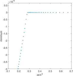
(a) Minimum of entries in $\bar{L}_{h}^{-1}$

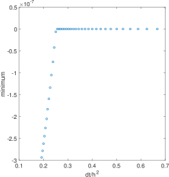
(b) Minimum of entries in $L_{h}^{-1}$

Figure 5: Minimum of all entries of $\bar{L}_{h}^{-1}$ and $L_{h}^{-1}$ on $16\times 32$ mesh with different time steps.

6 Concluding remarks

In this paper we have proven that the simplest fourth order accurate finite difference implementation of $C^{0}$-$Q^{2}$ finite element method is monotone thus satisfies a discrete maximum principle for solving a variable coefficient problem $-\nabla\cdot(a(x,y)\nabla u)+c(x,y)u=f$ under some suitable mesh constraints. The main results in this paper can be used to construct high order spatial discretization preserving positivity or maximum principle for solving time-dependent diffusion problems implicitly by backward Euler time discretization.

Appendix A M-Matrix factorization for discrete Laplacian

The matrix form of (9) can be written as $\frac{1}{h^{2}}\bar{L}_{h}\bar{\mathbf{u}}=\bar{\mathbf{f}}$. As an example, if there are seven interior grid points in the mesh for $(0,1)$, then the matrix $\bar{L}_{h}$ is given by

$$\bar{L}_{h}=\begin{pmatrix}1&&&&&&&\\ -1&2&-1&&&&&&\\ \frac{1}{4}&-2&\frac{7}{2}&-2&\frac{1}{4}&&&&\\ &&-1&2&-1&&&&\\ &&\frac{1}{4}&-2&\frac{7}{2}&-2&\frac{1}{4}&&\\ &&&&-1&2&-1&&\\ &&&&\frac{1}{4}&-2&\frac{7}{2}&-2&\frac{1}{4}\\ &&&&&&-1&2&-1\\ &&&&&&&&1\end{pmatrix}$$

The matrix $\bar{L}_{h}$ can be written as a product of two nonsingular M-matrices $\bar{L}_{h}=M_{1}M_{2}$ where

$$M_{1}=\begin{pmatrix}1&&&&&&&&\\ &1&&&&&&&\\ &-\frac{1}{4}&1&-\frac{1}{4}&&&&&\\ &&&1&&&&&\\ &&&-\frac{1}{4}&1&-\frac{1}{4}&&&\\ &&&&&1&&&\\ &&&&&-\frac{1}{4}&1&-\frac{1}{4}&\\ &&&&&&&1&\\ &&&&&&&&1\end{pmatrix},M_{2}=\begin{pmatrix}1&&&&&&&&&\\ -1&2&-1&&&&&&&\\ &-\frac{3}{2}&3&-\frac{3}{2}&&&&&\\ &&-1&2&-1&&&&\\ &&&-\frac{3}{2}&3&-\frac{3}{2}&&&\\ &&&&-1&2&-1&&\\ &&&&&-\frac{3}{2}&3&-\frac{3}{2}&\\ &&&&&&-1&2&-1\\ &&&&&&&&1\end{pmatrix}.$$

Such a factorization is not unique and it does not seem to have further physical or geometrical meanings.

For the scheme (11), we can find two linear operators $\mathcal{A}_{1}$ and $\mathcal{A}_{2}$ are with their matrix representations $A_{1}$ and $A_{2}$ being nonsingular M-matrices, such that $\mathcal{L}_{h}(\bar{\mathbf{u}})=\mathcal{A}_{2}(\mathcal{A}_{1}(\bar{\mathbf{u}}))$.

Definition of $\mathcal{A}_{1}$ is given as

• At boundary points:

  $$v_{i,j}=\mathcal{A}_{1}(\bar{\mathbf{u}})_{i,j}=u_{i,j}:=g_{ij}.$$

• At interior knots:

  $$v_{i,j}=\mathcal{A}_{1}(\bar{\mathbf{u}})_{i,j}=u_{i,j}.$$

• At interior cell center:

  $$v_{i,j}=\mathcal{A}_{1}(\bar{\mathbf{u}})_{i,j}=2u_{i,j}-\frac{1}{4}u_{i-1,j}-\frac{1}{4}u_{i+1,j}-\frac{1}{4}u_{i,j-1}-\frac{1}{4}u_{i,j+1}.$$

• At interior edge center (an edge parallel to x-axis):

  $$v_{i,j}=\mathcal{A}_{1}(\bar{\mathbf{u}})_{i,j}=-\frac{1}{6}u_{i-1,j}+\frac{4}{3}u_{i,j}-\frac{1}{6}u_{i+1,j}.$$

• At interior edge center (an edge parallel to y-axis):

  $$v_{i,j}=\mathcal{A}_{1}(\bar{\mathbf{u}})_{i,j}=-\frac{1}{6}u_{i,j-1}+\frac{4}{3}u_{i,j}-\frac{1}{6}u_{i,j+1}.$$

Definition of $\mathcal{A}_{2}$ is given as:

• At boundary points:

  $$\mathcal{A}_{2}(\bar{\mathbf{v}})_{i,j}=v_{i,j}.$$

• At an interior knot:

  $$\mathcal{A}_{2}(\bar{\mathbf{v}})_{i,j}=-\frac{3}{2}v_{i-1,j}+3v_{i,j}-\frac{3}{2}v_{i+1,j}-\frac{3}{2}v_{i,j-1}+3v_{i,j}-\frac{3}{2}v_{i,j+1}$$

• At an interior cell center:

  $$\mathcal{A}_{2}(\bar{\mathbf{v}})_{i,j}=2v_{i,j}-\frac{3}{8}v_{i-1,j}-\frac{3}{8}v_{i+1,j}-\frac{3}{8}v_{i,j-1}-\frac{3}{8}v_{i,j+1}-\frac{1}{8}v_{i-1,j+1}-\frac{1}{8}v_{i+1,j+1}-\frac{1}{8}v_{i-1,j-1}-\frac{1}{8}v_{i+1,j+1}.$$

• At an interior edge center (an edge parallel to x-axis):

  $$\mathcal{A}_{2}(\bar{\mathbf{v}})_{i,j}=-\frac{7}{16}v_{i-1,j}+\frac{15}{4}v_{i,j}-\frac{7}{16}v_{i+1,j}-v_{i,j+1}-v_{i,j-1}-\frac{3}{16}v_{i-1,j-1}-\frac{3}{16}v_{i+1,j-1}$$

  $$-\frac{3}{16}v_{i-1,j+1}-\frac{3}{16}v_{i+1,j+1}-\frac{1}{32}v_{i-1,j+2}-\frac{1}{32}v_{i+1,j+2}-\frac{1}{32}v_{i-1,j-2}-\frac{1}{32}v_{i+1,j-2}.$$

• At an interior edge center (an edge parallel to y-axis):

  $$\mathcal{A}_{2}(\bar{\mathbf{v}})_{i,j}=-\frac{7}{16}v_{i,j-1}+\frac{15}{4}v_{i,j}-\frac{7}{16}v_{i,j+1}-v_{i+1,j}-v_{i-1,j}-\frac{3}{16}v_{i-1,j-1}-\frac{3}{16}v_{i-1,j+1}$$

  $$-\frac{3}{16}v_{i+1,j-1}-\frac{3}{16}v_{i+1,j+1}-\frac{1}{32}v_{i+2,j-1}-\frac{1}{32}v_{i+2,j+1}-\frac{1}{32}v_{i-2,j-1}-\frac{1}{32}v_{i-2,j+1}.$$

It is straightforward to verify that $\mathcal{L}_{h}(\bar{\mathbf{u}})=\mathcal{A}_{2}(\bar{\mathbf{v}})$ where $\bar{\mathbf{v}}=\mathcal{A}_{1}(\bar{\mathbf{u}})$. Obviously, matrices of $\mathcal{A}_{1}$ and $\mathcal{A}_{2}$ have positive diagonal entries and nonpositive off-diagonal entries. Moreover, $\mathcal{A}_{1}(\mathbf{1})\geq 0$ and $\mathcal{A}_{2}(\mathbf{1})\geq 0$ thus $A_{1}$ and $A_{2}$ satisfy the row sum conditions in Theorem 3.4. So $A_{1}$ and $A_{2}$ are both nonsingular $M$-matrices and the matrix representation of $\mathcal{L}_{h}$ is $A_{2}A_{1}$. However, this kind of M-matrix factorization cannot be extended to the variable coefficient case.

Appendix B

Proof B.1 (Proof of Theorem 4.3).

If $c(x)\equiv 0$, then (25) reduces to

$$(28a_{i-1}+20a_{i+1})a_{i}+4a_{i+1}a_{i-1}>9a^{2}_{i-1}+3a^{2}_{i+1}.$$

A convenient sufficient condition is to require

$$52\min\{a_{i-1}^{2},a_{i}^{2},a^{2}_{i+1}\}>12\max\{a^{2}_{i-1},a^{2}_{i},a^{2}_{i+1}\},$$

which is equivalent to

$$\frac{\max\{a_{i-1},a_{i},a_{i+1}\}}{\min\{a_{i-1},a_{i},a_{i+1}\}}<\sqrt{\frac{13}{3}}.$$

Let $a(x^{1})=\max\{a_{i-1},a_{i},a_{i+1}\}$ and $a(x^{2})=\min\{a_{i-1},a_{i},a_{i+1}\}$. Then the inequality above is equivalent to

$$\frac{a(x^{1})-a(x^{2})}{a(x^{2})}<\frac{\sqrt{39}-3}{3}.$$

By the Mean Value Theorem, there is some $\xi\in(x_{i-1},x_{i+1})$ such that $a(x^{1})-a(x^{2})=a^{\prime}(\xi)(x^{2}-x^{1})$. Since $|x^{2}-x^{1}|\leq 2h$, we have

$$|a(x^{1})-a(x^{2})|\leq\max\limits_{x\in(x_{i-1},x_{i+1})}\left|a^{\prime}(x)\right|2h.$$

Thus a sufficient condition is to require

$$h\frac{\max\limits_{x\in(x_{i-1},x_{i+1})}\left|a^{\prime}(x)\right|}{\min\limits_{x\in(x_{i-1},x_{i+1})}a(x)}<\frac{\sqrt{39}-3}{6}.$$

For $c(x)\geq 0$, (25) reduces to

$$(28a_{i-1}+20a_{i+1})a_{i}+4a_{i+1}a_{i-1}>9a^{2}_{i-1}+3a^{2}_{i+1}+4h^{2}c_{i}(3a_{i-1}-4a_{i}+3a_{i+1}),$$

for which a sufficient condition is

(30) $$13\min\limits_{I_{i}}a^{2}(x)>3\max\limits_{I_{i}}a^{2}(x)+h^{2}c_{i}(6\max\limits_{I_{i}}a(x)-4\min\limits_{I_{i}}a(x)).$$

One sufficient condition for (30) is to have

$$\exists\lambda\in(0,1),h^{2}c_{i}(6\max\limits_{I_{i}}a(x)-4\min\limits_{I_{i}}a(x))<13(1-\lambda)\min\limits_{I_{i}}a^{2}(x),\quad 3\max\limits_{I_{i}}a^{2}(x)<13\lambda\min\limits_{I_{i}}a^{2}(x).$$

By similar discussions above, a sufficient condition for $3\max\limits_{I_{i}}a^{2}(x)<13\lambda\min\limits_{I_{i}}a^{2}(x)$ is to have $\lambda>\frac{3}{13}$ and

$$h\frac{\max\limits_{x\in I_{i}}\left|a^{\prime}(x)\right|}{\min\limits_{x\in I_{i}}a(x)}<\frac{\sqrt{39\lambda}-3}{6}.$$

The inequality (30) is also equivalent to

$$10\min\limits_{I_{i}}a^{2}(x)>3(\max\limits_{I_{i}}a^{2}(x)-\min\limits_{I_{i}}a^{2}(x))+h^{2}c_{i}(6\max\limits_{I_{i}}a(x)-4\min\limits_{I_{i}}a(x)).$$

Let $a^{2}(x^{1})=\max\limits_{I_{i}}a^{2}(x)$ and $a^{2}(x^{2})=\min\limits_{I_{i}}a^{2}(x)$, then by the Mean Value Theorem on the function $a^{2}(x)$, there is some $\xi\in(x_{i-1},x_{i+1})$ such that

$$a^{2}(x^{1})-a^{2}(x^{1})=2a(\xi)a^{\prime}(\xi)(x^{1}-x^{2})\leq 4h\max\limits_{I_{i}}a(x)\max\limits_{I_{i}}|a^{\prime}(x)|.$$

So it suffices to have

$$10\min\limits_{I_{i}}a^{2}(x)>12h\max\limits_{I_{i}}a(x)\max\limits_{I_{i}}|a^{\prime}(x)|+h^{2}c_{i}(6\max\limits_{I_{i}}a(x)-4\min\limits_{I_{i}}a(x)),$$

which can be simplified to

$$2h\max\limits_{I_{i}}|a^{\prime}(x)|+h^{2}c_{i}(1-\frac{2}{3}\frac{\min\limits_{I_{i}}a(x)}{\max\limits_{I_{i}}a(x)})<\frac{5}{3}\frac{\min\limits_{I_{i}}a^{2}(x)}{\max\limits_{I_{i}}a(x)}.$$

If $a(x)\equiv a>0$, it is straightforward to verify that (25) is equivalent to $hc_{i}<5a.$

Proof B.2 (Proof of Theorem 4.4).

For a smooth coefficient $a(x)$, by Taylor’s Theorem,

$$a(x+h)=a(x)+ha^{\prime}(x)+\frac{1}{2}h^{2}a^{\prime\prime}(\xi_{1}),\xi_{1}\in[x,x+h],$$

$$a(x-h)=a(x)-ha^{\prime}(x)+\frac{1}{2}h^{2}a^{\prime\prime}(\xi_{2}),\xi_{2}\in[x-h,x].$$

With the Intermediate Value Theorem for $a^{\prime\prime}(x)$, we get

$$a(x)=\frac{1}{2}[a(x+h)+a(x-h)-h^{2}a^{\prime\prime}(\xi)],\quad\xi\in(\xi_{2},\xi_{1})\subset[x-h,x+h].$$

Thus we can rewrite $a_{i}$ as $a_{i}=\frac{1}{2}(a_{i-1}+a_{i+1}-d_{i}h^{2})$ where

$$d_{i}:=\frac{a_{i-1}+a_{i+1}-2a_{i}}{h^{2}}=a^{\prime\prime}(\xi),\textrm{ for some }\xi\in(x_{i-1},x_{i+1}).$$

If $c(x)\equiv 0$, then (25) reduces to $(28a_{i-1}+20a_{i+1})a_{i}+4a_{i+1}a_{i-1}>9a^{2}_{i-1}+3a^{2}_{i+1}.$ Introducing an arbitrary number $\lambda\in(0,2]$, it is equivalent to

$$4a_{i+1}a_{i-1}+(4-2\lambda)a_{i}(7a_{i-1}+5a_{i+1})+2\lambda a_{i}(7a_{i-1}+5a_{i+1})>9a^{2}_{i-1}+3a^{2}_{i+1,}$$

$$(12\lambda+4)a_{i+1}a_{i-1}+(4-2\lambda)a_{i}(7a_{i-1}+5a_{i+1})+(7\lambda-9)a_{i-1}^{2}+(5\lambda-3)a_{i+1}^{2}$$

$$>\lambda h^{2}d_{i}(7a_{i-1}+5a_{i+1}),$$

$$(\frac{4}{\lambda}-2)a_{i}+a_{i-1}\frac{(5\lambda-3)\theta^{2}+(12\lambda+4)\theta+(7\lambda-9)}{\lambda(5\theta+7)}>h^{2}d_{i},\quad\theta=\frac{a_{i+1}}{a_{i-1}},$$

$$\left(\frac{4}{\lambda}-2\right)a_{i}+\left(\frac{\frac{41}{5}\theta-9}{\lambda(5\theta+7)}+1\right)a_{i-1}+\left(1-\frac{3}{5\lambda}\right)a_{i+1}>h^{2}d_{i}.$$

Notice that $\frac{\frac{41}{5}\theta-9}{5\theta+7}>-\frac{9}{7}$. By taking $\frac{9}{7}\leq\lambda\leq 2$, it suffices to require

(31) $$(1-\frac{9}{7\lambda})a_{i-1}+(\frac{4}{\lambda}-2)a_{i}+(1-\frac{3}{5\lambda})a_{i+1}>h^{2}d_{i},$$

as a sufficient condition of the above inequalities. If $a(x)$ is a concave function, then it satisfies $a(x_{i})=a(\frac{x_{i-1}+x_{i-1}}{2})\geq\frac{1}{2}a(x_{i-1})+\frac{1}{2}a(x_{i+1}),$ which implies $a_{i-1}+a_{i+1}-2a_{i}\leq 0$, thus (31) holds trivially. Otherwise, (31) holds for $\lambda=\frac{9}{7}$ if the following mesh constraint is satisfied:

$$h^{2}\max_{x\in(x_{i-1},x_{i+1})}a^{\prime\prime}(x)<\frac{74}{45}\min\{a_{i-1},a_{i},a_{i+1}\}.$$

If $c(x)\geq 0$, for any $\lambda\in(0,2]$, (25) is equivalent to

$$(12\lambda+4)a_{i+1}a_{i-1}+(4-2\lambda)a_{i}(7a_{i-1}+5a_{i+1})+(7\lambda-9)a_{i-1}^{2}+(5\lambda-3)a_{i+1}^{2}$$

(32) $$>\lambda h^{2}d_{i}(7a_{i-1}+5a_{i+1})+4h^{2}c_{i}(a_{i-1}+a_{i+1}+2d_{i}h^{2}).$$

If assuming $d_{i}h^{2}\leq\frac{74}{45}\min\{a_{i-1},a_{i},a_{i+1}\}$, then $d_{i}h^{2}\leq\lambda_{1}a_{i-1}+\lambda_{2}a_{i+1}$ for any two positive numbers $\lambda_{1},\lambda_{2}$ satisfying $\lambda_{1}+\lambda_{2}=\frac{74}{45}$. In particular, for $\lambda_{1}=\frac{563}{540}$, we get $d_{i}h^{2}\leq\frac{563}{540}a_{i-1}+\frac{65}{108}a_{i+1}$, which implies

$$a_{i-1}+a_{i+1}+2d_{i}h^{2}\leq\frac{119}{270}(7a_{i-1}+5a_{i+1}).$$

By replacing $a_{i-1}+a_{i+1}+2d_{i}h^{2}$ by the inequality above in (32), we get a sufficient condition for (32) as following:

$$(12\lambda+4)a_{i+1}a_{i-1}+(4-2\lambda)a_{i}(7a_{i-1}+5a_{i+1})+(7\lambda-9)a_{i-1}^{2}+(5\lambda-3)a_{i+1}^{2}$$

(33) $$>\lambda h^{2}d_{i}(7a_{i-1}+5a_{i+1})+4h^{2}c_{i}\frac{119}{270}(7a_{i-1}+5a_{i+1}).$$

Similar to the derivation of (31), we can derive a sufficient condition of (33) as

$$h^{2}\left(1.5c_{i}+\max_{x\in(x_{i-1},x_{i+1})}a^{\prime\prime}(x)\right)<\frac{74}{45}\min\{a_{i-1},a_{i},a_{i+1}\}.$$

If $d_{i}\leq 0$, then a sufficient condition for (32) is

$$\frac{(12\lambda+4)a_{i+1}a_{i-1}+(4-2\lambda)a_{i}(7a_{i-1}+5a_{i+1})+(7\lambda-9)a_{i-1}^{2}+(5\lambda-3)a_{i+1}^{2}}{a_{i-1}+a_{i+1}}\\ >4h^{2}c_{i},$$

from which we can derive a sufficient condition as

$$4h^{2}c_{i}<(7\lambda-9)a_{i-1}+(5-\frac{5}{2}\lambda)a_{i}+(5\lambda-3)a_{i+1},$$

for which a sufficient condition by setting $\lambda=2$ is $h^{2}c_{i}<3\min\{a_{i-1},a_{i},a_{i+1}\}.$

Proof B.3 (Proof of Theorem 4.6).

Since (27a) and (28) are equivalent to

$$4(7a_{i-1,j}+5a_{i+1,j})a_{ij}+4a_{i-1,j}a_{i+1,j}+16a_{ij}(a_{i,j-1}+a_{i,j+1})$$

$$>9a^{2}_{i-1,j}+3a^{2}_{i+1,j}+12(a_{i-1,j}+a_{i+1,j})(a_{i,j-1}+a_{i,j+1})+4(3a_{i-1,j}-4a_{ij}+3a_{i+1,j})h^{2}c_{ij}$$

and

$$8a_{i-1,j}a_{i+1,j}+2a_{ij}a_{i-1,j}+4a_{ij}(a_{i,j-2}+4a_{i,j-1}+18a_{i,j}+4a_{i,j+1}+a_{i,j+2})>18a^{2}_{i-1,j}+6a^{2}_{i+1,j}$$

$$+14a_{ij}a_{i+1,j}+3(a_{i-1,j}+a_{i+1,j})(a_{i,j-2}+4a_{i,j-1}+4a_{i,j+1}+a_{i,j+2})+8(3a_{i-1,j}-4a_{ij}+3a_{i+1,j})h^{2}c_{ij}.$$

A sufficient condition is to require

(34) $$7\min_{I_{ij}}a(x)^{2}>5\max_{I_{ij}}a(x)^{2}+\frac{2}{3}(3\max_{I_{ij}}a(x)-2\min_{I_{ij}}a(x))h^{2}c_{ij}$$

for all cell centers $x_{ij}$ of cell $I_{ij}=[x_{i-1},x_{i+1}]\times[y_{i-1},y_{i+1}]$, and the following mesh constraints for all edge centers $x_{ij}$:

(35) $$61\min_{J_{ij}}a(x)^{2}>49\max_{J_{ij}}a(x)^{2}+8(3\max_{J_{ij}}a(x)-2\min_{J_{ij}}a(x))h^{2}c_{ij},$$

where we $J_{ij}$ is the union of two cells: if $x_{ij}$ is an edge center of an edge parallel to $x$-axis, then $J_{ij}=I_{i,j-1}\cup I_{i,j+1}$; if $x_{ij}$ is an edge center of an edge parallel to $y$-axis, then $J_{ij}=I_{i-1,j}\cup I_{i+1,j}$. Notice that (35) implies (34), thus it suffices to have (35) only.

References

- [1] O. Axelsson and L. Kolotilina, Monotonicity and discretization error estimates, SIAM Journal on Numerical Analysis, 27 (1990), pp. 1591–1611.
- [2] E. Bohl and J. Lorenz, Inverse monotonicity and difference schemes of higher order. a summary for two-point boundary value problems, Aequationes Mathematicae, 19 (1979), pp. 1–36.
- [3] F. Bouchon, Monotonicity of some perturbations of irreducibly diagonally dominant m-matrices, Numerische Mathematik, 105 (2007), pp. 591–601.
- [4] J. Bramble and B. Hubbard, On the formulation of finite difference analogues of the Dirichlet problem for Poisson’s equation, Numerische Mathematik, 4 (1962), pp. 313–327.
- [5] J. Bramble and B. Hubbard, On a finite difference analogue of an elliptic boundary problem which is neither diagonally dominant nor of non-negative type, Journal of Mathematics and Physics, 43 (1964), pp. 117–132.
- [6] J. H. Bramble, Fourth-order finite difference analogues of the Dirichlet problem for Poisson’s equation in three and four dimensions, Mathematics of Computation, 17 (1963), pp. 217–222.
- [7] J. H. Bramble and B. E. Hubbard, New monotone type approximations for elliptic problems, Mathematics of Computation, 18 (1964), pp. 349–367.
- [8] I. Christie and C. Hall, The maximum principle for bilinear elements, International Journal for Numerical Methods in Engineering, 20 (1984), pp. 549–553.
- [9] P. G. Ciarlet, Discrete maximum principle for finite-difference operators, Aequationes mathematicae, 4 (1970), pp. 338–352.
- [10] P. G. Ciarlet and P.-A. Raviart, Maximum principle and uniform convergence for the finite element method, Computer Methods in Applied Mechanics and Engineering, 2 (1973), pp. 17–31.
- [11] A. Drăgănescu, T. Dupont, and L. Scott, Failure of the discrete maximum principle for an elliptic finite element problem, Mathematics of computation, 74 (2005), pp. 1–23.
- [12] L. C. Evans, Partial Differential Equations, vol. 019, American Mathematical Society, 2010.
- [13] P. J. Ferket and A. A. Reusken, A finite difference discretization method for elliptic problems on composite grids, Computing, 56 (1996), pp. 343–369.
- [14] W. Höhn and H. D. Mittelmann, Some remarks on the discrete maximum-principle for finite elements of higher order, Computing, 27 (1981), pp. 145–154.
- [15] J. Karátson and S. Korotov, Discrete maximum principles for fem solutions of some nonlinear elliptic interface problems, Int. J. Numer. Anal. Model, 6 (2009), pp. 1–16.
- [16] S. Korotov, M. Křížek, and J. Šolc, On a Discrete Maximum Principle for Linear FE Solutions of Elliptic Problems with a Nondiagonal Coefficient Matrix, in Numerical Analysis and Its Applications, S. Margenov, L. G. Vulkov, and J. Waśniewski, eds., Berlin, Heidelberg, 2009, Springer Berlin Heidelberg, pp. 384–391.
- [17] D. Kuzmin, M. J. Shashkov, and D. Svyatskiy, A constrained finite element method satisfying the discrete maximum principle for anisotropic diffusion problems, Journal of Computational Physics, 228 (2009), pp. 3448–3463.
- [18] S. K. Lele, Compact finite difference schemes with spectral-like resolution, Journal of Computational Physics, 103 (1992), pp. 16–42.
- [19] H. Li, S. Xie, and X. Zhang, A high order accurate bound-preserving compact finite difference scheme for scalar convection diffusion equations, SIAM Journal on Numerical Analysis, 56 (2018), pp. 3308–3345.
- [20] H. Li and X. Zhang, On the fourth order accuracy of the finite difference implementation of - finite element method for elliptic equations, arXiv preprint arXiv:1904.01179, (2019).
- [21] Z. Li and K. Ito, Maximum principle preserving schemes for interface problems with discontinuous coefficients, SIAM Journal on Scientific Computing, 23 (2001), pp. 339–361.
- [22] J. Lorenz, Zur inversmonotonie diskreter probleme, Numerische Mathematik, 27 (1977), pp. 227–238.
- [23] G. Payette, K. Nakshatrala, and J. Reddy, On the performance of high-order finite elements with respect to maximum principles and the nonnegative constraint for diffusion-type equations, International Journal for Numerical Methods in Engineering, 91 (2012), pp. 742–771.
- [24] R. J. Plemmons, M-matrix characterizations. I-nonsingular M-matrices, Linear Algebra and its Applications, 18 (1977), pp. 175–188.
- [25] T. Qin and C.-W. Shu, Implicit positivity-preserving high-order discontinuous galerkin methods for conservation laws, SIAM Journal on Scientific Computing, 40 (2018), pp. A81–A107.
- [26] J. Shen, T. Tang, and J. Yang, On the maximum principle preserving schemes for the generalized Allen–Cahn equation, Commun. Math. Sci, 14 (2016), pp. 1517–1534.
- [27] T. Tang and J. Yang, Implicit-explicit scheme for the Allen-Cahn equation preserves the maximum principle, J. Comput. Math, 34 (2016), pp. 471–481.
- [28] T. Vejchodskỳ, Angle conditions for discrete maximum principles in higher-order FEM, in Numerical Mathematics and Advanced Applications 2009, Springer, 2010, pp. 901–909.
- [29] T. Vejchodskỳ and P. Šolín, Discrete maximum principle for a 1D problem with piecewise-constant coefficients solved by hp-FEM, Journal of Numerical Mathematics, 15 (2007), pp. 233–243.
- [30] T. Vejchodskỳ and P. Šolín, Discrete maximum principle for higher-order finite elements in 1D, Mathematics of Computation, 76 (2007), pp. 1833–1846.
- [31] J. Whiteman, Lagrangian finite element and finite difference methods for poisson problems, in Numerische Behandlung von Differentialgleichungen, Springer, 1975, pp. 331–355.
- [32] J. Xu, Y. Li, S. Wu, and A. Bousquet, On the stability and accuracy of partially and fully implicit schemes for phase field modeling, Computer Methods in Applied Mechanics and Engineering, 345 (2019), pp. 826–853.
- [33] J. Xu and L. Zikatanov, A monotone finite element scheme for convection-diffusion equations, Mathematics of Computation, 68 (1999), pp. 1429–1446.