Statistical properties of thermal neutron capture cross section calculated with randomly generated resonance parameters

Abstract

We investigated the probability distribution of the thermal neutron capture cross section ($\sigma_{\rm th}$) deduced stochastically with the resonance parameters randomly sampled from Wigner and Porter-Thomas distributions. We found that the typical probability distribution has an asymmetric shape. While there is a long tail on the large $\sigma_{\rm th}$ side due to a resonance happening to be close to the thermal energy, the multi-resonance contribution considerably reduces the probability on the small $\sigma_{\rm th}$ side. We also found that the probability distributions have a similar shape if nuclei have an average resonance spacing sufficiently larger than an average radiation width. We compared the typical probability distribution with the distribution of the experimental values of 193 nuclei, and found a good agreement between them.

I Introduction

In a low-energy neutron reaction model, the compound nuclear process is usually described by resonance theories or the statistical model depending on the incident neutron energy. Practically, resonance theories are used to fit experimental cross sections and extract the resonance parameters. In general, if there is no experimental data, the calculated cross sections using the resonance theories hardly make sense, because the theoretical prediction of the resonance parameter with high accuracy is extremely difficult due to the complexity of excited states of the compound nucleus around the neutron separation energy. In a higher neutron incident energy region, where neighbor resonances overlap each other within their width, the resonance structure of the cross sections disappears. In such region, cross sections can be characterized by the statistical average of the resonance parameters.

An approach to deduce cross sections in the resonance region from the statistical properties of the resonance parameters was made by Rochman $et$ $al$. 1 . They generated resonance parameters by random sampling from the $\chi^{2}$ distribution for the neutron width, and Wigner distribution 9 for the resonance energy spacing. This approach is similar to the numerical method to account for the width fluctuation in the averaged cross section, which was performed by Moldauer 4 .

The thermal neutron capture cross section $\sigma_{\rm th}$ is important for various nuclear applications and has been experimentally measured for most of stable nuclei. Although $\sigma_{\rm th}$ data of radioactive nuclei are even required for particular applications, such as the evaluation of the transmutation system for the radioactive nuclear wastes, experimental data is limited compared with the stable nuclei. If there is no experimental data, $\sigma_{\rm th}$ is often calculated using the systematics 2 ; 3 . However, $\sigma_{\rm th}$ is considered to be governed by the resonance that is closest to the thermal neutron energy i.e. the neutron separation energy of the compound nucleus, and drastically changed even with a slight variation of the resonance energy or width. Therefore, the systematics would give only a rough estimation of $\sigma_{\rm th}$. Actually, they never predict extremely large $\sigma_{\rm th}$ observed for some nuclei, such as ¹³⁵Xe (2.6 $\times$ $10^{6}$ b) and ¹⁵⁷Gd (2.5 $\times$ $10^{5}$ b). If one applies the stochastic approach presented by Rochman et al. 1 , such extremely large $\sigma_{\rm th}$ can happen to be obtained if a resonance is generated at a energy close to the thermal energy. Of course that does not necessarily happen, and the generated resonance sometimes appear far away from the thermal energy. Accordingly, such a calculated cross section must have a large uncertainty that originates from the statistical fluctuation of the resonance parameters.

Although such kind of stochastic approach will be an optional way to calculate the neutron reaction data in the resolved resonance region for nuclei that have no or scarce experimental data, it is important to clarify unavoidable uncertainty attributed to the statistical fluctuation at the same time. Therefore, in this study, we aim to figure out the uncertainty in $\sigma_{\rm th}$ predicted from the statistical property of the resonance parameters. For this purpose, we deduced the probability distribution of $\sigma_{\rm th}$ from stochastically prepared sets of resonance parameters with their known statistical properties, and investigated its property. The probability distributions of the cross sections in the resolved resonance region deduced by such a stochastic method have been already utilized in the recent evaluated nuclear data library 11 . To figure out the feature of the numerically obtained distribution, we also derive the analytical expression of the probability distribution by applying a single-resonance approximation, in which only one resonance closest to the neutron threshold is included.

Practically, we calculate $\sigma_{\rm th}$ using Breit-Winger formula with the resonance parameters randomly sampled from Porter-Thomas 10 and Wigner 9 distributions. The probability distribution of $\sigma_{\rm th}$ is numerically derived by calculating $\sigma_{\rm th}$ repeatedly using resonance parameter sets generated from different random seeds. Porter-Thomas and Wigner distributions are characterized by the averages of the resonance widths and spacing, respectively, which are required as input of the present calculation. We intend to apply the present method to the nuclei that have no experimental data in future, and in that case those parameters must be calculated theoretically. However, in this paper, we focus on nuclei whose $\sigma_{\rm th}$ and averages of the resonance spacing and widths are known to confirm the validity of our method.

This paper is organized as follows. In Sec. II, numerical procedure to calculate the probability distribution of $\sigma_{\rm th}$ is explained, and the analytical expression of the probability distribution derived by applying the single-resonance approximation is presented. Properties of the calculated probability distribution of $\sigma_{\rm th}$ are discussed in Sec. III, and Sec. IV summarizes this work.

II Theoretical framework

We use Breit-Wigner formula to calculate the s-wave radiative capture cross section at thermal energy $E_{\rm th}$,

$$\sigma_{\rm th}=\frac{\pi}{k^{2}}\sum_{j=I-\frac{1}{2}}^{j=I+\frac{1}{2}}\sum_{i\in j}^{N}\frac{g_{j}\Gamma_{ni}\Gamma_{\gamma i}}{\left(E_{0}-E_{i}\right)^{2}+\left(\frac{1}{2}\Gamma_{i}\right)^{2}}.$$ (1)

In this equation, $\Gamma_{ni},\Gamma_{\gamma i},\Gamma_{i},$ $E_{i}$, and $N$ are the neutron width, the radiative width, the total width, the energy of the i-th resonance with total spin $j$, and the number of resonances, respectively. Fission, alpha and other particle emission channels are not considered in the present formulation. The wave number $k=\sqrt{2\mu E_{0}}/\hbar$ and $E_{0}=m_{t}/\left(m_{n}+m_{t}\right)E_{{\rm th}}$, where $m_{n},m_{t},$ and $\mu$ are the neutron mass, the target mass and the reduced mass, respectively. The spin statistical factor $g_{j}$ is given by

$$g_{j}=\frac{2j+1}{2(2I+1)},$$ (2)

where $I$ is the total spin of the target nucleus. In our framework, the resonance energy is a random variable given by Wigner distribution 9 ,

$$P_{\rm e}(x^{j})=\frac{\pi}{2}x^{j}e^{-\frac{\pi}{4}(x^{j})^{2}},x^{j}=\frac{E_{i+1}^{j}-E_{i}^{j}}{D_{0}^{j}},$$ (3)

with the average s-wave resonance spacing $D_{0}^{j}$. Since the experimental value of $D_{0}$ does not depend on $j$, we evaluate $D_{0}^{j}$ of $I\neq 0$ nuclei from the experimental $D_{0}$ by adopting Gaussian spin distribution with the spin dispersion parameter ${\rm s}^{2}$ of Mengoni-Nakajima 7 ,

$$W(E_{x},j) = \frac{2j+1}{2{\rm s}^{2}}\exp\left[-\frac{(j+\frac{1}{2})^{2}}{2{\rm s}^{2}}\right].$$ (4)

Using Eq. (4), $D_{0}^{j}$ are calculated as

$$D_{0}^{I+\frac{1}{2}} = \frac{1+R_{I}}{R_{I}}D_{0},\hskip 5.69054ptD_{0}^{I-\frac{1}{2}}=(1+R_{I})D_{0},$$ (5)

$$R_{I} = \frac{W(S_{n},I+\frac{1}{2})}{W(S_{n},I-\frac{1}{2})}.$$

The neutron width is related with the reduced neutron width as

$$\Gamma_{ni}=\sqrt{E_{0}}\Gamma_{ni}^{l=0},$$ (6)

and the reduced neutron width is a random variable with Porter-Thomas distribution 9 ,

$$P_{\rm w}\left(\Gamma_{ni}^{l=0}\right)=\frac{1}{\sqrt{2\pi\Gamma_{ni}^{l=0}\langle\Gamma_{n0}\rangle}}\exp\left(-\frac{\Gamma_{ni}^{l=0}}{2\langle\Gamma_{n0}\rangle}\right).$$ (7)

We calculate the average s-wave neutron reduced width $\langle\Gamma_{n0}\rangle$ using the experimental strength function $S_{0}$ defined as

$$S_{0}=\frac{\langle g\Gamma_{n0}\rangle}{D_{0}}=\frac{1}{\Delta E}\sum_{j}\sum_{i\in j}g_{j}\Gamma_{ni}^{l=0}.$$ (8)

For $I=0$ nucleus, $\langle\Gamma_{n0}\rangle=S_{0}D_{0}$. For $I\neq 0$ nucleus, we suppose that $\Gamma_{ni}^{l=0}$ is not dependent on $j$, and write Eq. (8) as

$$S_{0}=\frac{1}{D_{0}}\left(g_{I-\frac{1}{2}}\langle\Gamma_{n0}\rangle\frac{D_{0}}{D_{0}^{I-\frac{1}{2}}}+g_{I+\frac{1}{2}}\langle\Gamma_{n0}\rangle\frac{D_{0}}{D_{0}^{I+\frac{1}{2}}}\right).$$ (9)

The average neutron width $\langle\Gamma_{n0}\rangle$ is calculated using Eq. (9) with the experimental $S_{0}$. For $\Gamma_{\gamma i}$, we assume that

$$\Gamma_{\gamma i}\sim\langle\Gamma_{\gamma 0}\rangle.$$ (10)

In the calculation of actual nuclei, we use the experimental data of $D_{0}$, $\langle\Gamma_{\gamma 0}\rangle$ and $S_{0}$, which are taken from the compilation of Mughabghab 5 . We calculate the probability distribution of 193 nuclei for which all of the resonance parameters and $\sigma_{\rm th}$ are given by Mughabghab. Since the fission channel is not taken into account in the present formulation, the nuclei heavier than ²⁰⁹Bi are excluded. We also arbitrarily exclude the nuclei lighter than ²⁷Al because it is expected that the statistical property of the resonance parameter is invalid for nuclei with low level densities.

As explained above, the resonance parameters are random variables in the present framework, and therefore, $\sigma_{\rm th}$ has a probability distribution. We calculate it in two ways; one is a numerical way that is the repetitive calculation of $\sigma_{\rm th}$ using randomly sampled resonance parameters (Sec. II.1), and another is an analytical way using the single-resonance approximation (Sec. II.2).

II.1 Numerical solution

First of all, we set an initial resonance at $-\frac{N}{2}\times D_{0}$ so that it starts from a sufficiently small energy. Then the next resonance energy is randomly sampled from Winger distribution of Eq. (3). For each resonance, the width is randomly sampled from Porter-Thomas distribution of Eq. (7). For $I\neq 0$ nucleus, $j=I-\frac{1}{2}$ and $j=I+\frac{1}{2}$ resonances are generated independently. The generation of the resonance is repeated until the number of resonance reaches to $N$, and then we calculate ${\sigma_{\rm th}}$ using the set of the resonance parameters and Breit-Wigner formula. By repeating this procedure, we obtain many samples of $\sigma_{\rm th}$. With sufficiently large number of samples, the probability distribution of $\sigma_{\rm th}$, which is denoted by $P_{\sigma}^{\rm M}$ (M stands for multi-resonance), is obtained.

To discuss the statistical property of $P_{\sigma}^{\rm M}$, we calculate the median $\sigma_{\rm md}^{M}$ and the dispersion $V$, which is defined as

$$V=\int_{-\infty}^{\infty}(x-\log\sigma_{\rm md}^{\rm M})^{2}P_{\sigma}^{\rm M}(x)dx,\hskip 8.53581ptx=\log\sigma_{\rm th}.$$ (11)

It is noted that the definition is different from the usual one of the standard deviation. The dispersion $V$ is also used to check the convergence of the numerical procedure. If the number of trials is small, $V$ values obtained from different random seeds are significantly different from each other because of the statistical fluctuation. We fixed the number of trials at $10^{7}$ to obtain $P_{\sigma}^{\rm M}$ for most calculations in this paper. Then the variation of $V$ caused by the statistical fluctuation is estimated to be less than 0.5$\%$.

It is noted that $P_{\sigma}^{\rm M}$ is dependent on the number of resonances $N$. We used $N=50$ in this paper, and confirmed that $V$ calculated using $N=100$ has less than 1$\%$ difference with that using $N=50$ in the calculation of ¹²⁰Sn shown in Sec. III. The dependence of $P_{\sigma}^{\rm M}$ on $N$ is also discussed there.

II.2 Analytical solution with single-resonance approximation

To understand the property of $\sigma_{\rm th}$, we present the formulation with the single-resonance approximation. This approximation enables us to express the probability distribution of $\sigma_{\rm th}$ in an analytical form and provides us a deeper insight into its properties.

Supposing that $\sigma_{\rm th}$ is dominated by the first resonance, and the thermal energy and the total width are small compared to the resonance energy, Eq. (1) is approximated as

$$\sigma_{\rm th} \simeq \frac{\pi}{k^{2}}\frac{g_{j}\Gamma_{n1}\Gamma_{\gamma 1}}{E_{1}^{2}},$$

$$\propto \frac{\Gamma_{n1}^{l=0}}{E_{1}^{2}}.$$

Here $E_{1}$ is the energy of the resonance that is closest to $E_{0}$. Note that both positive and negative resonances can be $E_{1}$. In this equation, $E_{1}$ and $\Gamma_{n1}^{l=0}$ are random variables.

We found that if the resonance energy spacing is given by Wigner distribution, the probability distribution of $E_{1}$ can be given by the normal distribution with the standard deviation of $d=D_{0}^{2}/2\pi$ for $I=0$ nucleus. For $I\neq 0$ nuclei, we approximate $E_{1}$ with the normal distribution same with $I=0$ case using $j$-independent $D_{0}$.

Since the probability distribution of $E_{1}$ is the normal distribution, that of $E_{1}^{2}$ is the $\chi^{2}$ distribution of one degree of freedom. Then $\sigma_{\rm th}$ is found to be proportional to the ratio of two $\chi^{2}$ distributions with Porther-Thomas distribution, which is generally known to be given by F-distribution. As a consequence of the above explained conversions of the statistical variables (the detail is given in Appendix), the probability distribution of $\sigma_{\rm th}$ is given as

$$P_{\sigma}^{\rm S}(\sigma_{\rm th}) = \frac{1}{\pi\sigma_{\rm th}}\left(\sqrt{\frac{\sigma_{\rm th}}{\sigma_{{\rm md}}^{\rm S}}}+\sqrt{\frac{\sigma_{{\rm md}}^{\rm S}}{\sigma_{\rm th}}}\right)^{-1},$$ (13)

$$\sigma_{{\rm md}}^{{\rm S}} = \frac{2\pi^{2}}{k^{2}}\sqrt{E_{0}}\frac{\langle\Gamma_{n0}\rangle\langle\Gamma_{\gamma 0}\rangle}{D_{0}^{2}},$$ (14)

where $\sigma_{{\rm md}}^{{\rm S}}$ corresponds to the median of the probability distribution (S stands for single resonance). Since the expectation value of $\sigma_{\rm th}$ is dominated by the tail of the probability distribution in extremely large $\sigma_{\rm th}$ region, we use the median, not the average, in what follows.

We express $P_{\sigma}^{\rm S}$ as well as $P_{\sigma}^{\rm M}$ in terms of log $\sigma_{\rm th}$ instead of $\sigma_{\rm th}$. It was found that $P_{\sigma}^{\rm S}(\log\sigma_{\rm th})$ is expressed by a hyperbolic secant function centered at $\log\sigma_{{\rm md}}^{{\rm S}}$,

$$P_{\sigma}^{\rm S}(\log\sigma_{\rm th})=\frac{1}{2\pi}{\rm sech}\left(\frac{\log\sigma_{\rm th}-\log\sigma_{{\rm md}}^{{\rm S}}}{2}\right).$$ (15)

It is clear from this equation that the averages of the resonance spacing and widths, which are characteristic of nuclei, changes only the center of the probability distribution. In other words, $P_{\sigma}^{\rm S}(\log\frac{\sigma_{\rm th}}{\sigma_{\rm md}^{\rm S}})$ is identical for all nuclei.

III results

III.1 Probability distributions for specific nuclei

In this section, we show the probability distributions $P_{\sigma}^{\rm M}$ and $P_{\sigma}^{\rm S}$ for specific nuclei. It is noted that $P_{\sigma}^{\rm S}$ is essentially different from $P_{\sigma}^{\rm M}$ due the absence of the multi-resonance contribution. In Fig. 1, $P_{\sigma}^{\rm M}$ and $P_{\sigma}^{\rm S}$ as function of $\log\sigma_{\rm th}$ calculated using the experimental values of the averages of the resonance spacing and widths are shown. First of all, it is clearly seen that both $P_{\sigma}^{\rm M}(\log\sigma_{\rm th})$ and $P_{\sigma}^{\rm S}(\log\sigma_{\rm th})$ are distributed over extremely wide range of several order of magnitude. This broad distribution is naturally regarded from the property of resonance nature.

As for $P_{\sigma}^{\rm S}(\log\sigma_{\rm th})$, it is just a hyperbolic secant function, which has a symmetric shape and long tails both in small and large $\sigma_{\rm th}$ regions. The peak of the distribution corresponds to $\sigma_{{\rm md}}^{\rm S}$, which is 0.01 b for ¹²⁰Sn. While we chose ¹²⁰Sn as an example here, the shape of $P_{\sigma}^{\rm S}(\log\sigma_{\rm th})$ is the same for all nuclei, as mentioned in the last paragraph of the Sec. II.2.

Although it is expected that $\sigma_{\rm th}$ is dominated by the first resonance, $P_{\sigma}^{\rm M}(\log\sigma_{\rm th})$ shows a considerably different distribution from $P_{\sigma}^{\rm S}(\log\sigma_{\rm th})$. To show the dependence on the number of resonance $N$, $P_{\sigma}^{\rm M}$ calculated using $N=4,16,50$ are compared in Fig. 1. While the tail of $P_{\sigma}^{\rm S}(\log\sigma_{\rm th})$ extends to the small cross section side, $P_{\sigma}^{\rm M}(\log\sigma_{\rm th})$ has a steep slope on the left shoulder. Comparing the calculations with different $N$, it can be seen $P_{\sigma}^{\rm M}$ with the larger $N$ has a less probability in the smaller $\sigma_{\rm th}$ side. On the other hand, $P_{\sigma}^{\rm M}(\log\sigma_{\rm th})$ and $P_{\sigma}^{\rm S}(\log\sigma_{\rm th})$ are similar in the larger $\sigma_{\rm th}$ region. They have peaks at approximately the same $\sigma_{\rm th}$, and overlaps in the region of $\sigma_{\rm th}>1$ b. In $P_{\sigma}^{\rm M}(\log\sigma_{\rm th})$, the second and subsequent resonances have considerable contributions to $\sigma_{\rm th}$ if its value is small, while the first resonance has a dominant contribution to the emergence of a large $\sigma_{\rm th}$. Consequently, the multi-resonance contribution considerably reduces the statistical fluctuation in small values of $\sigma_{\rm th}$.

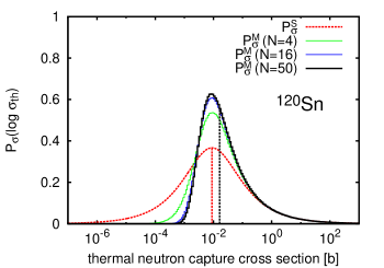
Figure 1: Probability distributions $P_{\sigma}^{\rm M}(\log\sigma_{\rm th})$ and $P_{\sigma}^{\rm S}(\log\sigma_{\rm th})$. For $P_{\sigma}^{\rm M}(\log\sigma_{\rm th})$, calculations using the number of resonance $N$=4,16,50 are compared.

We also calculated $P_{\sigma}^{\rm M}$ of various nuclei, and found that the difference of the averages of the resonance spacing and widths barely affect the shape of $P_{\sigma}^{\rm M}(\log\sigma_{\rm th})$, if the condition $D_{0}\gg\langle\Gamma_{\gamma 0}\rangle$ is satisfied. To show this, we compare shapes of $P_{\sigma}^{\rm M}(\log\sigma_{\rm th})$ for different nuclei by normalizing $\sigma_{\rm th}$ to medians of distributions. For simplicity, we use the following notation

$$\sigma_{\rm N}=\frac{\sigma_{\rm th}}{\sigma_{{\rm md}}}.$$ (16)

In Fig. 2 (a), $P_{\sigma}^{\rm M}(\log\sigma_{\rm N})$ of several nuclei are shown as a function of $\sigma_{\rm N}$. We also show the ratio to the $P_{\sigma}^{\rm M}(\log\sigma_{\rm N})$ of ¹²⁰Sn in Fig. 2 (b). Comparing the results of ¹²⁰Sn and ¹⁵⁴Gd, which have $D_{0}=1485$ eV and 13.8 eV, respectively, $P_{\sigma}^{\rm M}(\log\sigma_{\rm N})$ are very similar in spite of the large difference of $D_{0}$. Only a small difference is found in $\sigma_{N}<1$ and $\sigma_{N}>10^{4}$ as seen in Fig. 2 (b). For most of the calculated 193 nuclei, the differences are even smaller than this case or the same degree. Exception is found in ¹⁵²Eu and ¹⁹²Ir, which have extremely small $D_{0}$ of 0.25 eV and 0.64 eV, respectively. The distributions of ¹⁵²Eu and ¹⁹²Ir are significantly narrower range than the typical distribution represented by that of ¹²⁰Sn. In Sec. III.2, we show that such noticeable difference appears if nuclei have $D_{0}$ comparable to $\langle\Gamma_{\gamma 0}\rangle$.

Differences between $P_{\sigma}^{\rm M}(\log\sigma_{\rm N})$ for $I=0$ and $I\neq$ 0 nuclei are also extremely small. Comparing $P_{\sigma}^{\rm M}(\log\sigma_{\rm N})$ of ¹¹⁹Sn ($I=1/2$) and ¹²⁰Sn ($I=0$), only a minute difference is found around $\sigma_{N}\sim 0.1$.

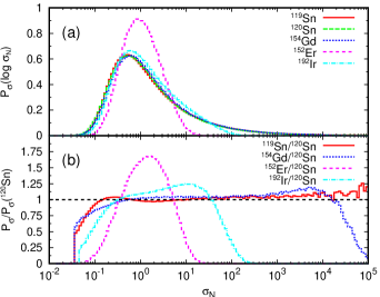
Figure 2: (a) Probability distribution $P_{\sigma}^{\rm M}(\log\sigma_{\rm N})$ of ¹¹⁹Sn, ¹²⁰Sn, ¹⁵²Eu, ¹⁵⁴Gd, and (b) the ratio of those to $P_{\sigma}^{\rm M}(\log\sigma_{\rm N})$ of ¹²⁰Sn.

III.2 Dependence on averages of resonance spacing and widths

We investigated the dependence of $P_{\sigma}^{\rm M}(\log\sigma_{\rm N})$ on the averages of the resonance spacing and widths. To quantify a change of $P_{\sigma}^{\rm M}(\log\sigma_{\rm N})$, the dispersion $V$ defined by Eq.(11) is discussed in this section. Further discussion using the quantities with higher-moments is given in Sec. III.3. We also discuss $\sigma_{{\rm md}}^{\rm M}$ normalized to $\sigma_{{\rm md}}^{\rm S}$ ($\sigma_{{\rm md}}^{\rm M}/\sigma_{{\rm md}}^{\rm S}$). By this quantity, we can measure the change of $P_{\sigma}^{\rm M}$ relative to $P_{\sigma}^{\rm S}$, which is independent of the averages of the resonance spacing and widths. If $\sigma_{{\rm md}}^{\rm M}/\sigma_{{\rm md}}^{\rm S}$ is smaller (lager) than 1, it means that $P_{\sigma}^{\rm M}$ concentrated in the small (large) cross section side relative to $P_{\sigma}^{\rm S}$.

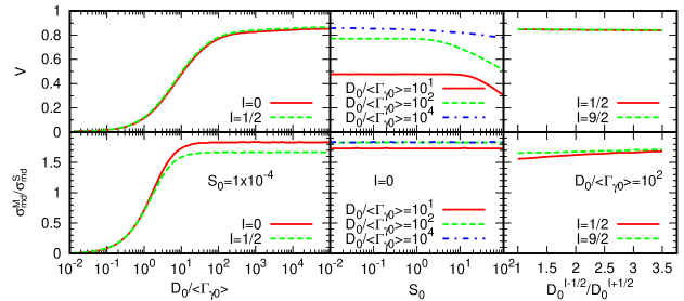
Figure 3: Dependence of $P_{\sigma}^{\rm M}(\log\sigma_{\rm N})$ on the averages of the resonance spacing, widths and the target spin $I$. Calculated $\sigma_{{\rm md}}^{\rm M}/\sigma_{{\rm md}}^{\rm S}$ and $V$ as functions of $D_{0}/\langle\Gamma_{\gamma 0}\rangle$, $S_{0}$ and $D_{0}^{I-1/2}/D_{0}^{I+1/2}$ are shown in the top and bottom panels, respectively. Results shown in the left, middle and right panels are obtained using $S_{0}=1$, $I$=0 and $D_{0}/\langle\Gamma_{\gamma 0}\rangle$=100, respectively. In all calculations, $\langle\Gamma_{\gamma 0}\rangle$ is fixed at 0.1 eV.

We calculated $P_{\sigma}^{\rm M}$ using various $D_{0}$ and $S_{0}$ for the target spin $I$=0 and $I=1/2$ cases. To see how the $j$-dependence of $D_{0}$ affects $P_{\sigma}^{\rm M}$, the ratio $D_{0}^{I-1/2}/D_{0}^{I+1/2}$ is also varied. In Fig. 3, the calculated $\sigma_{{\rm md}}^{\rm M}/\sigma_{{\rm md}}^{\rm S}$ and $V$ as a function of the averages of the resonance spacing and widths are shown. The calculation is carried out by fixing $\langle\Gamma_{\gamma 0}\rangle=$0.1 eV. We have confirmed that the result shown in Fig. 3 does not change even if $\langle\Gamma_{\gamma 0}\rangle=$1 eV.

In the left panels of Fig. 3, the results with $S_{0}$ fixed at 1$\times 10^{-4}$ are shown as a function of $D_{0}/\langle\Gamma_{\gamma 0}\rangle$. In $D_{0}/\langle\Gamma_{\gamma 0}\rangle>100$ region, $\sigma_{{\rm md}}^{\rm M}/\sigma_{{\rm md}}^{\rm S}$ have almost constant values of 1.8 and 1.7 for $I=0$ and $I=1/2$ cases, respectively. Similarly, $V$ is almost converged at 0.8 in this region. In $D_{0}/\langle\Gamma_{\gamma 0}\rangle<100$ region, a significant decrease of $V$ is seen. Around $D_{0}/\langle\Gamma_{\gamma 0}\rangle\sim 100$, where $V$ starts to decrease, the tail of $P_{\sigma}^{\rm M}$ in the large $\sigma_{\rm th}$ side is slightly reduced as in the case of ¹⁹²Ir. The median is rather insensitive to the variation of the tail distribution, therefore $\sigma_{{\rm md}}^{\rm M}/\sigma_{{\rm md}}^{\rm S}$ is still constant around $D_{0}/\langle\Gamma_{\gamma 0}\rangle\sim 100$. If $D_{0}$ becomes comparable to $\langle\Gamma_{\gamma 0}\rangle$, $P_{\sigma}^{\rm M}$ distributes in a significantly narrower $\sigma_{\rm th}$ range, as in the case of ¹⁵²Eu.

The middle panels of Fig. 3 show the results as a function of $S_{0}$ with $I=0$. If $\langle\Gamma_{n0}\rangle$ is much lager than $\langle\Gamma_{\gamma 0}\rangle$, a total width is often dominated by a neutron width. In this case, $P_{\sigma}^{\rm M}(\log\sigma_{\rm N})$ changes from the typical distribution. This can be seen from the middle top panel, in which the reduction of $V$ becomes noticeable in the large $S_{0}$ region. The degree of the change is not so large, therefore $\sigma_{{\rm md}}^{\rm M}/\sigma_{{\rm md}}^{\rm S}$ shows a constancy against the change of $S_{0}$.

Although $P_{\sigma}^{\rm M}$ is also dependent on $I$, it has an small influence on the shape of the distribution, but slightly change the median of the distribution. From the left bottom panel of Fig.3, the difference between $\sigma_{{\rm md}}^{\rm M}/\sigma_{{\rm md}}^{\rm S}$ calculated with $I=0$ and $I=1/2$ can be seen. The difference between the results with $I=1/2$ and $I=9/2$ is also visible in the right bottom panel. These differences are mainly because $j$-independent $D_{0}$ and the spin statistical factor $g_{j}=$ 1 are assumed in the calculation of $\sigma_{\rm md}^{\rm S}$ if $I$ is not equal to 0. Therefore, the variation of $\sigma_{{\rm md}}^{\rm M}/\sigma_{{\rm md}}^{\rm S}$ is largest if the nucleus has $I=1/2$, because the difference between $g_{I-\frac{1}{2}}$ and $g_{I+\frac{1}{2}}$ is largest in this case. On the other hand, there is an extremely small change in $V$ calculated using different $I$, as shown in the left top and the right top panel.

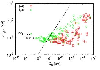
Figure 4: Distribution of $D_{0}$ and $\langle\Gamma_{\gamma 0}\rangle$ for 193 nuclei with $I=0$ and $I\neq 0$. The dashed line indicates $D_{0}/\langle\Gamma_{\gamma 0}\rangle=100$ line. The symbols corresponding to ¹⁵²Eu and ¹⁹²In are indicated by the arrows.

As discussed above, one of the conditions that cause a significant change in $P_{\sigma}^{\rm M}(\log\sigma_{\rm N})$ is that $D_{0}$ becomes comparable to $\langle\Gamma_{\gamma 0}\rangle$. To see whether actual nuclei satisfy this condition or not, the experimentally known $D_{0}$ and $\langle\Gamma_{\gamma 0}\rangle$ of 193 stable nuclei are plotted in Fig. 4. We can see that the most of nuclei are in the region of $D_{0}/\langle\Gamma_{\gamma 0}\rangle>100$, where $\sigma_{{\rm md}}^{\rm M}/\sigma_{{\rm md}}^{\rm S}$ and $V$ are almost constant. Namely, the most of stable nuclei have very similar $P_{\sigma}^{\rm M}$, which are characterized with $\sigma_{{\rm md}}^{\rm M}/\sigma_{{\rm md}}^{\rm S}\sim 1.8$ (I=0) or 1.7 (I$\neq$0) and $V\sim 0.8$. The constancy of $\sigma_{{\rm md}}^{\rm M}/\sigma_{{\rm md}}^{\rm S}$ will be convenient for a practical use, because $\sigma_{{\rm md}}^{\rm M}$ can be calculated easily from $\sigma_{{\rm md}}^{\rm S}$ without numerically calculating $P_{\sigma}^{\rm M}$ from many samples. In $D_{0}/\langle\Gamma_{\gamma 0}\rangle<100$ side, there are approximately 30 nuclei. Among these nuclei, ¹⁵²Eu has the smallest $D_{0}/\langle\Gamma_{\gamma 0}\rangle$ of 1.56. While only ¹⁵²Eu have extremely large $D_{0}$ comparable to $\langle\Gamma_{\gamma 0}\rangle$ among stable nuclei, it may not be a case for unstable nuclei. For example, since neutron separation energies of proton-rich nuclei are generally higher than those of stable nuclei, they may have extremely large $D_{0}$.

III.3 General properties of probability distributions

In this section, the general property of the probability distribution is discussed in terms of the skewness $\beta_{1}^{1/2}$ and the kurtosis $\beta_{2}$, which are defined by third and fourth central moments with the expectation value $\mu$, respectively,

$$\mu = \int_{-\infty}^{\infty}xP_{\sigma}^{\rm M}(x)dx,\hskip 14.22636pt$$

$$\mu_{r} = \int_{-\infty}^{\infty}(x-\mu)^{r}P_{\sigma}^{\rm M}(x)dx,\hskip 14.22636ptx=\log\sigma_{\rm th},$$

$$\beta_{1}^{1/2} = \frac{\mu_{3}}{\mu_{2}^{3/2}},\hskip 14.22636pt\beta_{2}=\frac{\mu_{4}}{\mu_{2}^{2}}-3.$$ (17)

The skewness $\beta_{1}^{1/2}$ has a sensitivity to the asymmetry of the distribution. The kurtosis is more sensitive to the tailedness of the distribution than the quantities with lower central moments. Both quantities become 0 for the normal distribution in the present definition.

In Fig. 5, the calculated $\beta_{1}^{1/2}$, $\beta_{2}$ and $\mu^{2}$ are shown. In $D_{0}/\langle\Gamma_{\gamma 0}\rangle>100$ region, while $\mu^{2}$ comes close to the constant, $\beta_{1}^{1/2}$ and $\beta_{2}$ are still increasing, which indicates that the tail of the distribution is growing in this region. The positive sign of $\beta_{1}^{1/2}$ means that the distribution is leaning to the left side. As already discussed in the previous section, the distribution drastically changes around $D_{0}/\langle\Gamma_{\gamma 0}\rangle\sim 10$, and $\beta_{2}$ becomes negative there. The negative sign of $\beta_{2}$ means that the tail of the distribution is even suppressed from that of the normal distribution.

In $D_{0}/\langle\Gamma_{\gamma 0}\rangle<1$ region, all quantities come close to 0, and the distribution converges to the normal distribution. In that condition, the following expressions may be valid. Supposing $E_{i}^{2}\ll 1/4\Gamma_{i}^{2}$ and $\Gamma_{\gamma i}\gg\Gamma_{ni}$ in Eq. (1), $\sigma_{\rm th}$ is approximated as

$$\sigma_{\rm th}\simeq\frac{\pi}{k^{2}}\frac{\langle\Gamma_{\gamma 0}\rangle}{E_{0}^{2}+\frac{1}{4}\langle\Gamma_{\gamma 0}\rangle^{2}}\sum_{i}^{N_{c}}\Gamma_{ni},$$ (18)

where $N_{c}$ is the number of the last resonance which satisfies the above conditions. If $N_{c}$ is sufficiently large, the probability distribution of $\sigma_{\rm th}$ is approximated with the normal distribution from the central limit theorem,

$$P_{\sigma}^{M}(\sigma_{\rm th}) \simeq \frac{1}{\sqrt{2\pi\mu_{2}}}\exp\left(-\frac{(\sigma_{\rm th}-\mu)^{2}}{2\mu_{2}}\right).$$ (19)

Here $\mu$ and $\mu_{2}$ are given as

$$\mu = \frac{\pi}{k^{2}}\frac{\langle\Gamma_{\gamma 0}\rangle}{E_{0}^{2}+\frac{1}{4}\langle\Gamma_{\gamma 0}\rangle^{2}}\sqrt{E_{0}}\langle\Gamma_{n0}\rangle N_{c},\hskip 5.69054pt\mu_{2}=\mu^{2}\frac{2}{N_{c}}.$$ (20)

From these equations, it is clear that the standard deviation of the normal distribution $\mu_{2}$ decreases as $N_{c}$ increases. The uncertainty arising from the statistical fluctuation of the resonance parameters is minimized in this case.

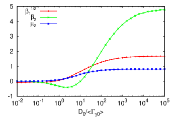
Figure 5: Skewness $\beta_{1}^{1/2}$ and kurtosis $\beta_{2}$ of $P_{\sigma}^{\rm M}$ as a function of $D_{0}/\langle\Gamma_{\gamma 0}\rangle$.

III.4 Comparison with the distribution of experimental data

Finally, we compare $P_{\sigma}^{\rm M}$ with the experiments, to confirm the validity of the present method. In principle, we cannot discuss the validity of $P_{\sigma}^{\rm M}$ for each nucleus, because there is only one experimental value for each nucleus to be compared with. Therefore, we utilize the finding that $P_{\sigma}^{\rm M}(\log\sigma_{\rm N})$ are similar for most of nuclei. We normalize the experimental $\sigma_{\rm th}$ of 193 stable nuclei to the calculated $\sigma_{{\rm md}}^{\rm M}$, in order to compare them with the typical $P_{\sigma}^{\rm M}(\log\sigma_{\rm N})$ calculated with the condition of $D_{0}/\langle\Gamma_{\gamma 0}\rangle=10^{3}$. Namely, we check the validity of one typical $P_{\sigma}^{\rm M}(\log\sigma_{\rm N})$ by comparing it with the distribution of 193 samples.

In Fig. 6 (a), $P_{\sigma}^{\rm M}(\log\sigma_{\rm N})$ with $D_{0}/\langle\Gamma_{\gamma 0}\rangle=10^{3}$ is compared with the distribution of 193 nuclei as a function of the experimentally measured $\sigma_{\rm th}$ normalized to the calculated $\sigma_{\rm md}^{\rm M}$. It is noted that $P_{\sigma}^{\rm M}(\log\sigma_{\rm N})$ for some of 193 nuclei in $D_{0}/\langle\Gamma_{\gamma 0}\rangle<100$ eV region are varied from a typical distribution, as discussed above. While the tails of the probability in the large $\sigma_{\rm th}$ region slightly shorten in these nuclei, such small variations are not important for the comparison with the distribution of the experimental data. Therefore, we also use the values of these nuclei for better statics. We can see a fair agreement between $P_{\sigma}^{\rm M}(\log\sigma_{\rm N})$ and the distribution of the experimental data. The agreement is even found in the extremely large $\sigma_{\rm th}$ region around $\sigma/\sigma_{{\rm md}}^{\rm M}\sim 10^{3}$ with four samples: ³⁵Cl, ¹¹³Cd, ¹⁵⁷Gd and ¹⁶⁴Dy.

We also plot the cumulative probability in Fig. 6 (b). We can see a good agreement between the calculated cumulative probability and the cumulative number of the experimental data. This results support the validity of the major part of $P_{\sigma}^{\rm M}(\log\sigma_{\rm N})$.

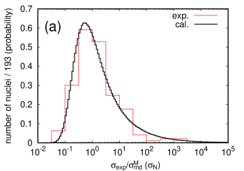
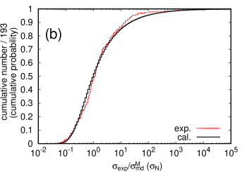
Figure 6: (a) Distribution ((b) cumulative distribution) of the nuclei as a function of the experimental $\sigma_{\rm th}$ normalized to $\sigma_{{\rm md}}^{\rm M}$ compared with $P_{\sigma}^{\rm M}\log(\sigma_{\rm N})$. The vertical axis is the number (cumulative number) of nuclei divided by the total number of nuclei, which are comparable to the probability (cumulative probability).

IV Summary

In this study, we investigated the probability distribution of the thermal neutron capture cross section $\sigma_{\rm th}$ calculated from the statistical properties of the resonance parameters. In practice, the probability distribution was deduced numerically using the resonance parameters randomly sampled from Wigner and Porter-Thomas distributions. In the case of the single-resonance approximation, the analytical expression of the probability distribution was derived.

We revealed that to what extent $\sigma_{\rm th}$ can be varied due to the statistical fluctuation of the resonance parameters from the probability distributions. It is important that the multi-resonance contribution significantly narrows the distribution and suppresses the emergence of a extremely small $\sigma_{\rm th}$. Another important finding is that shapes of the probability distributions are very similar for nuclei that have $D_{0}$ sufficiently larger than $\langle\Gamma_{\gamma_{0}}\rangle$. The typical probability distribution for most of stable nuclei was compared with the distribution of the experimentally observed $\sigma_{\rm th}$. The validity of the present method was confirmed from a good agreement between them.

This study presents a fundamental knowledge to utilize the stochastic method to estimate $\sigma_{\rm th}$ for nuclei that have no available experimental data. The probability distribution can be used to evaluate the uncertainty in the calculated $\sigma_{\rm th}$. The methodology used in this study is not limited to the calculation of $\sigma_{\rm th}$, however will be useful to evaluate uncertainty arising from a statistical treatment of the resolved resonances in practical applications.

*

Appendix A

Equation (13) is easily derived from the conversion of the random variables, which is well known for the normal and $\chi^{2}$ distributions. We suppose that $E_{1}$ has Gaussian distribution with zero mean,

$$P_{\rm se}(E_{1})=\frac{1}{\sqrt{2\pi d}}\exp\left(-\frac{E_{1}^{2}}{2d}\right).$$ (21)

If we take the standard deviation $d=D_{0}^{2}/2\pi$, $P_{\rm se}(E_{1})$ agrees with the probability distribution of the first resonance numerically calculated using Wigner distribution. By converting the random variable $E_{1}$ to $E_{1}^{2}$, it becomes $\chi^{2}$ distribution of one degree of freedom,

$$P_{\rm se}(E_{1}^{2})=\frac{1}{\sqrt{2\pi dE_{1}^{2}}}\exp\left(-\frac{E_{1}^{2}}{2d}\right).$$ (22)

Then the probability distribution of $\Gamma_{n1}^{l=0}/E_{1}^{2}$ is calculated as

$$P_{\rm f}(Y) = \int_{0}^{\infty}P_{w}(YZ)P_{se}(Z)ZdZ,$$

$$= \frac{1}{\pi Y}\left(\sqrt{\frac{d}{\langle\Gamma_{n0}\rangle}Y}+\sqrt{\frac{\langle\Gamma_{n0}\rangle}{d}\frac{1}{Y}}\right)^{-1},$$

$$Y = \Gamma_{n1}^{l=0}/E_{1}^{2},\hskip 14.22636ptZ=E_{1}^{2}.$$

The further conversion of the random variable $Y$ to $\sigma_{\rm th}=\frac{2}{k^{2}}\sqrt{E_{0}}\langle\Gamma_{\gamma 0}\rangle Y$ yields $P_{\sigma}^{\rm S}$ of Eq. (13). Equation (15) is derived by replacing the exponential function emerged from the conversion of $\sigma_{\rm th}$ to $\log\sigma_{\rm th}$

$$P_{\sigma}^{\rm S}(\log\sigma_{\rm th}) = \frac{\sqrt{\sigma_{{\rm md}}^{\rm S}}}{\pi}\left({\rm e}^{\frac{\log\sigma_{\rm th}}{2}}+\sigma_{{\rm md}}^{\rm S}{\rm e}^{-\frac{\log\sigma_{\rm th}}{2}}\right)^{-1},$$

with the hyperbolic functions.

It is easily confirmed that $\sigma_{\rm md}^{\rm S}$ in Eq. (13) corresponds to the median of $P_{\sigma}^{\rm S}$ from the following calculations. The cumulative distribution function of $\sigma_{\rm th}$ calculated form Eq. (13) is,

$$y=\int_{0}^{X}P_{\sigma}^{\rm S}(\sigma_{\rm th})d\sigma_{\rm th}=\frac{2}{\pi}{\rm tan^{-1}}\sqrt{\frac{X}{\sigma_{{\rm md}}^{\rm S}}},$$ (24)

and its inverse function is,

$$X=\sigma_{{\rm md}}^{\rm S}{\rm tan^{2}}\left(\frac{\pi}{2}y\right).$$ (25)

By putting the cumulative probability $y=0.5$ in Eq.(25), we find $X=\sigma_{\rm md}^{\rm S}$.

References

- (1) D. Rochman, A. J. Koning, J. Kopecky, J. -C. Sublet, P.Ribon, and M. Moxon, Annals of Nuclear Energy 51, 60 (2013).
- (2) E. P. Wigner, Oak Ridge National Laboratory Report ORNL-2309, p. 59, 1957.
- (3) P. A. Moldauer, Nucl. Phys. A 344, 185 (1980).
- (4) K. Shibata, J. Nucl. Sci. Technol. 51, 425 (2014).
- (5) J. Kopecky, M. G. Delfini, H. A. J. van der kamp and D. Nierop, Report ECN-C-952-051, 1992.
- (6) S. Kunieda et al.,J. Nucl. Sci. Technol. (to be published).
- (7) C. E. Porter and R. G. Thomas, Phys. Rev. 104, 483 (1956).
- (8) A. Mengoni and Y. Nakajima, J. Nucl. Sci. Technol. 31, 151 (1994).
- (9) S. F. Mughabghab, Atlas of neutron resonances: resonance parameters and thermal cross sections Z=1-100 (Elsevier, Amsterdam, 2006).