Iterative Alpha Expansion for estimating gradient-sparse signals from linear measurements
Abstract.
We consider estimating a piecewise-constant image, or a gradient-sparse signal on a general graph, from noisy linear measurements. We propose and study an iterative algorithm to minimize a penalized least-squares objective, with a penalty given by the “-norm” of the signal’s discrete graph gradient. The method proceeds by approximate proximal descent, applying the alpha-expansion procedure to minimize a proximal gradient in each iteration, and using a geometric decay of the penalty parameter across iterations. Under a cut-restricted isometry property for the measurement design, we prove global recovery guarantees for the estimated signal. For standard Gaussian designs, the required number of measurements is independent of the graph structure, and improves upon worst-case guarantees for total-variation (TV) compressed sensing on the 1-D and 2-D lattice graphs by polynomial and logarithmic factors, respectively. The method empirically yields lower mean-squared recovery error compared with TV regularization in regimes of moderate undersampling and moderate to high signal-to-noise, for several examples of changepoint signals and gradient-sparse phantom images.
1. Introduction
Consider an unknown signal observed via noisy linear measurements
We study the problem of estimating , under the assumption that its coordinates correspond to the vertices of a given graph , and is gradient-sparse. By this, we mean that
| (1) |
is much smaller than the total number of edges . Special cases of interest include the 1-D line graph, where variables have a sequential order and has a changepoint structure, and the 2-D lattice graph, where coordinates of represent pixels of a piecewise-constant image.
This problem has been studied since early pioneering works in compressed sensing [CRT06a, CRT06b, Don06]. Among widely-used approaches for estimating are those based on constraining or penalizing the total-variation (TV) semi-norm [ROF92], which may be defined (anisotropically) for a general graph as
These are examples of -analysis methods [EMR07, CENR11, NDEG13], which regularize the -norm of a general linear transform of rather than of its coefficients in an orthonormal basis. Related fused-lasso methods have been studied for different applications of regression and prediction in [TSR+05, Rin09, Tib11], other graph-based regularization methods for linear regression in [LMRW18, KG19], and trend-filtering methods regularizing higher-order discrete derivatives of in [KKBG09, WSST16].
Theoretical recovery guarantees for TV-regularization depend on the structure of the graph [NW13b, NW13a, CX15], and more generally on sparse conditioning properties of the pseudo-inverse for -analysis methods with sparsifying transform . For direct measurements , these and related issues were studied in [HR16, DHL17, FG18], which showed in particular that TV-regularization may not achieve the same worst-case recovery guarantees as analogous -regularization methods on certain graphs including the 1-D line. In this setting of , different computational approaches exist which may be used for approximately minimizing an -regularized objective on general graphs [BVZ99, KT02, XLXJ11].
Motivated by this line of work, we propose and study an alternative to TV-regularization for the problem with indirect linear measurements . Our procedure is based similarly on the idea of minimizing a possibly non-convex objective
| (2) |
for an edge-associated cost function . We will focus attention in this work on the specific choice of an -regularizer
| (3) |
which matches (1), although the algorithm may be applied with more general choices of metric edge cost. For the above edge cost, the resulting objective takes the form
We propose to minimize using an iterative algorithm akin to proximal gradient descent: For parameters and , the iterate is computed from via
For general graphs, the second update step for is only approximately computable in polynomial time. We apply the alpha-expansion procedure of Boykov, Veksler, and Zabih [BVZ99] for this task, first discretizing the continuous signal domain, as analyzed statistically in [FG18]. In contrast to analogous proximal methods in convex settings [BT09, PB14], where typically is fixed across iterations, we decay geometrically from a large initial value to ensure algorithm convergence. We call the resulting algorithm ITerative ALpha Expansion, or ITALE.
Despite being non-convex and non-smooth, we provide global recovery guarantees for a suitably chosen ITALE iterate . For example, under exact gradient-sparsity , if consists of
| (4) |
linear measurements with i.i.d. entries, then the ITALE iterate for the -regularizer (3) and a penalty value satisfies with high probability
| (5) |
More generally, we provide recovery guarantees when satisfies a certain cut-restricted isometry property, described in Definition 3.1 below. (In accordance with the compressed sensing literature, we state all theoretical guarantees for deterministic and possibly adversarial measurement error .)
Even for i.i.d. Gaussian design, we are not aware of previous polynomial-time algorithms which provably achieve this guarantees for either the 1-D line or the 2-D lattice. In particular, connecting with the above discussion, similar existing results for TV-regularization in noisy or noiseless settings require Gaussian measurements for the 2-D lattice and measurements for the 1-D line [NW13b, CX15]. In contrast, for lattice graphs of dimensions 3 and higher where the Laplacian is well-conditioned, as well as for more general -analysis methods where is a tight frame, optimal recovery guarantees for TV/-regularization hold with or measurements as expected [CENR11, NW13a, CX15]. ITALE provides this guarantee up to a constant factor, irrespective of the graph structure.
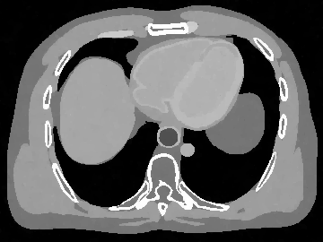
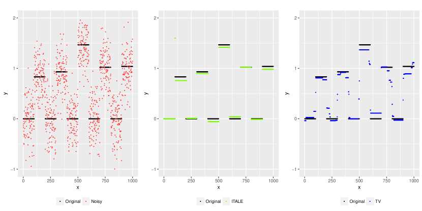
In practice, for sufficiently close to 1, we directly interpret the sequence of ITALE iterates as approximate minimizers of the objective function (2) for penalty parameters along a regularization path. We select the iterate using cross-validation on the prediction error for , and we use the final estimate . Figure 1 compares in simulation using the -regularizer (3) with (globally) minimizing the TV-regularized objective
| (6) |
with selected also using cross-validation. The example depicts a synthetic image of a human chest slice, previously generated by [GHG+17] using the XCAT digital phantom [SSM+10]. The design is an undersampled and reweighted Fourier matrix, using a sampling scheme described in Section 3 and similar to that proposed in [KW14] for TV-regularized compressed sensing. In a low-noise setting, a detailed comparison of the recovered images reveals that provides a sharper reconstruction than . As noise increases, becomes blotchy, while begins to lose finer image details. Quantitative comparisons of recovery error are provided in Section 4.2 and are favorable towards ITALE in lower noise regimes.


ITALE is similar to some methods oriented towards -regularized sparse regression and signal recovery [TG07, Zha11, BKM16], including notably the Iterative Hard Thresholding (IHT) [BD09] and CoSaMP [NT09] methods in compressed sensing. We highlight here several differences:
-
•
For sparsity in an orthonormal basis, forward stepwise selection and orthogonal matching pursuit provide greedy “” approaches to variable selection, also with provable guarantees [TG07, Zha11, EKDN18]. However, such methods do not have direct analogues for gradient-sparsity in graphs, as one cannot select a single edge difference to be nonzero without changing other edge differences.
-
•
IHT and CoSaMP enforce sparsity of in each iteration by projecting to the largest coordinates of , for user-specified . In contrast, ITALE uses a Lagrangian form that penalizes (rather than constrains) . This is partly for computational reasons, as we are not aware of fast algorithms that can directly perform such a projection step onto the (non-convex) set for general graphs. Our theoretical convergence analysis handles this Lagrangian form.
-
•
In contrast to more general-purpose mixed-integer optimization procedures in [BKM16], each iterate of ITALE (and hence also the full algorithm, for a polynomial number of iterations) is provably polynomial-time in the input size [FG18]. On our personal computer, for the image of Figure 1, computing the 60 iterates constituting a full ITALE solution path required about 20 minutes, using the optimized alpha-expansion code of [BK04].
While our theoretical focus is on -regularization, we expect that for certain regimes of undersampling and signal-to-noise, improved empirical recovery may be possible with edge costs interpolating between the and penalties. These are applicable in the ITALE algorithm and would be interesting to investigate in future work.
2. Model and algorithm
Let be a given connected graph on the vertices , with undirected edge set . We assume throughout that . For a signal vector , measurement matrix , and measurement errors , we observe
| (7) |
Denote by the discrete gradient matrix on the graph , defined111Here, we may fix an arbitrary ordering of the vertex pair for each edge. by
We study estimation of , assuming that has (or is well-approximated by a signal having) small exact gradient sparsity .
Our proposed algorithm is an iterative approach called ITALE, presented as Algorithm 1. It is based around the idea of minimizing the objective (2). In this objective, the cost function must satisfy the metric properties
| (8) |
but is otherwise general. Importantly, may be non-smooth and non-convex. The algorithm applies proximal descent, alternating between constructing a surrogate signal in line 3 and denoising this surrogate signal in line 4, discussed in more detail below.
Some intuition for is provided by considering the setting and , in which case
There are two sources of noise and in , the former expected to decrease across iterations as the reconstruction error decreases. A tuning parameter is applied to denoise in each iteration, where also decreases across iterations to match the noise level. Our theoretical analysis indicates to use a geometric rate of decay , starting from a large initial value .
ITALE yields iterates , which we directly interpret as recovered signals along a regularization path for different choices of in the objective (2). We choose such that the initial iterates oversmooth , and such that the final iterates undersmooth . We remark that an alternative approach would be to iterate lines 3 and 4 in Algorithm 1 until convergence for each , before updating to the next value . However, we find that this is not necessary in practice if is chosen close enough to 1, and our stated algorithm achieves a computational speed-up compared to this approach.
To perform the denoising in line 4, ITALE applies the alpha-expansion graph cut procedure from [BVZ99] to approximately solve the minimization problem
This sub-routine is denoted as , and is described in Algorithm 2 for completeness. At a high level, the alpha-expansion method encodes the above objective function in the structure of an edge-weighted augmented graph, and iterates over global moves that swap the signal value on a subset of vertices for a given new value by finding a minimum graph cut. The original alpha-expansion algorithm of [BVZ99] computes an approximate maximum-a-posteriori estimate in a discrete Potts model with a metric edge-cost satisfying (8). To apply this to a continuous signal domain, we restrict coordinate values of to a discrete grid
Here, is a small user-specified discretization parameter. As shown in [FG18, Lemma S2.1] (see also [BVZ99, Theorem 6.1]), the output has the deterministic guarantee
| (9) |
with the additional factor of 2 applying to the penalty on the right side. This guarantee is important for the theoretical recovery properties that we will establish in Section 3.
We make a few remarks regarding parameter tuning in practice:
-
•
Using conservative choices for (large), (close to 1), and (small) increases the total runtime of the procedure, but does not degrade the quality of recovery. In our experiments, we fix and set in each iteration to yield 300 grid values for in Algorithm 2.
-
•
We monitor the gradient sparsity across iterations, and terminate the algorithm when exceeds a certain fraction (e.g. 50%) of the total number of edges , rather than fixing .
- •
-
•
The most important tuning parameter is the iterate for which we take the final estimate . In practice, we apply cross-validation on the mean-squared prediction error for to select . Note that should be rescaled by the number of training samples in each fold, i.e. for 5-fold cross-validation with training sample size , we set instead of in the cross-validation runs.
3. Recovery guarantees
We provide in this section theoretical guarantees on the recovery error , where for a deterministic (non-adaptive) choice of iterate . Throughout this section, ITALE is assumed to be applied with the edge cost .
3.1. cRIP condition
Our primary assumption on the measurement design will be the following version of a restricted isometry property.
Definition 3.1.
Let , and let be any function satisfying and for all . A matrix satisfies the -cut-restricted isometry property (cRIP) if, for every with , we have
This definition depends implicitly on the structure of the underlying graph , via its discrete gradient matrix . Examples of the function are given in the two propositions below.
This condition is stronger than the usual RIP condition in compressed sensing [CRT06a, CRT06b] in two ways: First, Definition 3.1 requires quantitative control of for all vectors , rather than only those with sparsity for some specified . We use this in our analysis to handle regularization of in Lagrangian (rather than constrained) form. Second, approximate isometry is required for signals with small gradient-sparsity , rather than small sparsity . For graphs with bounded maximum degree, all sparse signals are also gradient-sparse, so this is indeed stronger up to a relabeling of constants. This requirement is similar to the D-RIP condition of [CENR11] for general sparse analysis models, and is also related to the condition of [NW13b] that satisfies the usual RIP condition, where is the inverse Haar-wavelet transform on the 2-D lattice.
Despite this strengthening of the required RIP condition, Definition 3.1 still holds for sub-Gaussian designs , where depends on the condition number of the design covariance. We defer the proof of the following result to Appendix B. For a random vector , we denote its sub-Gaussian norm as
and say that is sub-Gaussian if for a constant .
Proposition 3.2.
Let have i.i.d. rows , where and . Suppose that the largest and smallest eigenvalues of satisfy and for a constant . Then for any and some constant depending only on , with probability at least , the matrix satisfies -cRIP for the function
For large 2-D images, using Fourier measurements with matrix multiplication implemented by an FFT can significantly reduce the runtime of Algorithm 1. As previously discussed in [LDP07, NW13b, KW14], uniform random sampling of Fourier coefficients may not be appropriate for reconstructing piecewise-constant images, as these typically have larger coefficients in the lower Fourier frequencies. We instead study a non-uniform sampling and reweighting scheme similar to that proposed in [KW14] for total-variation compressed sensing, and show that Definition 3.1 also holds for this reweighted Fourier matrix.
For and both powers of 2, let be the 2-D discrete Fourier matrix on the lattice graph of size , normalized such that . We define this as the Kronecker product , where is the 1-D discrete Fourier matrix with entries
and is defined analogously. (Thus rows closer to in correspond to higher frequency components.) Let denote row of , where we index by pairs corresponding to the Kronecker structure. We define a sampled Fourier matrix as follows: Let be the probability mass function on given by
| (10) |
Define similarly on , and let . For a given number of measurements , draw , and set
| (11) |
Proposition 3.3.
Let be the 2-D lattice graph of size , where are powers of 2 and for a constant . Set and let be the matrix defined in (11). Then for some constants depending only on , and for any , with probability at least , satisfies the -cRIP with and
We defer the proof also to Appendix B. This proposition pertains to the complex analogue of Definition 3.1, where are allowed to be complex-valued, and denotes the complex -norm. For a real-valued signal , Algorithm 1 may be applied to by separating real and imaginary parts of into a real vector . The corresponding satisfies , so the same cRIP condition holds (in the real sense) for .
3.2. Recovery error bounds
To illustrate the idea of analysis, we first establish a result showing that ITALE can yield exact recovery in a setting of no measurement noise. We require to be gradient-sparse with coordinates belonging exactly to , as the ITALE output has this latter property. Discretization error will be addressed in our subsequent result.
Theorem 3.4.
Suppose and , and denote . Suppose satisfies -cRIP, where . Set , and choose tuning parameters
For some constants depending only on , if
then each iterate of Algorithm 1 satisfies
| (12) |
In particular, for all sufficiently large .
Thus, in this noiseless setting, the iterates exhibit linear convergence to the true signal . The required condition translates into a requirement of
measurements for having i.i.d. entries, by Proposition 3.2, or
weighted Fourier measurements for the 2-D lattice graph, as defined in Proposition 3.3. For these designs, -cRIP holds for where and .
Proof of Theorem 3.4.
Let be the partition of induced by the piecewise-constant structure of : Each element of corresponds to a connected subgraph of on which takes a constant value. Let similarly be the partitions induced by , and denote by the common refinement of . Defining the boundary
observe that each edge must be such that at least one of , , or takes different values at its two endpoints. Then
| (14) |
Let be the orthogonal projection onto the subspace of signals taking a constant value over each element of , and let . Then all belong to the range of , so an orthogonal decomposition yields
Applying this, the definition (in the noiseless setting )
and the condition to (13), we obtain
Applying the triangle inequality and ,
| (15) |
We derive from this two consequences: First, lower-bounding the left side by 0 and rearranging,
| (16) |
The condition (14) and definition of imply, for any , that . The definition of implies . Setting
we deduce from the -cRIP condition for that
| (17) |
Note that since and are both nonnegative and concave by Definition 3.1, we have
The function
is also increasing and concave, and by the above, its derivative at satisfies
Thus
| (18) |
Applying this and (17) to (16), we get
Rearranging gives
| (19) |
Second, applying the -cRIP condition for again, we have for every
So . Then, as , we get from (15) that
Taking the square-root and applying ,
Applying the definitions of and ,
Thus
| (20) |
We now claim by induction on that, if for a sufficiently small constant , then
| (21) |
for every . For , these are satisfied as and . Assume inductively that these hold for . Note that for any , nonnegativity and concavity yield . In particular, assuming (21) and applying and , we get for small enough that . Then applying (21) to (19), we get for a constant not depending on that
Then for small enough ,
Applying (21) and this bound to (20), for sufficiently small , we have
Applying , we obtain from this
This completes the induction and establishes (21) for every .
We now extend this result to provide a robust recovery guarantee in the presence of measurement and discretization error. The proof is an extension of the above argument, which we defer to Appendix A.
Theorem 3.5.
The quantity above is the combined measurement error and approximation error of by a discretized piecewise-constant signal . For any scaled such that it satisfies -cRIP with , and for with maximum degree , we get
This guarantee is similar to those for compressed sensing of sparse signals in [CRT06b, NT09, BD09]. If has exact gradient-sparsity , then also obtained by entrywise rounding to satisfies . Hence choosing further ensures
i.e. the discretization error is negligible in the above bound. The required number of measurements is the same as in Theorem 3.4 for the noiseless setting, which is for i.i.d. Gaussian designs. This is the claim (5) stated in the introduction.
4. Simulations
We compare using the edge cost (3) with minimizing the TV-regularized objective (6), for several signals on the 1-D and 2-D lattice graphs. We used software developed by [BK04] to implement the alpha-expansion sub-routine of Algorithm 2. To minimize the TV-regularized objective (6), we used the generalized lasso path algorithm from [Tib11] in the 1-D examples and the FISTA algorithm from [BT09] in the 2-D examples. All parameters were set as described in Section 2 for ITALE.
4.1. 1-D changepoint signals
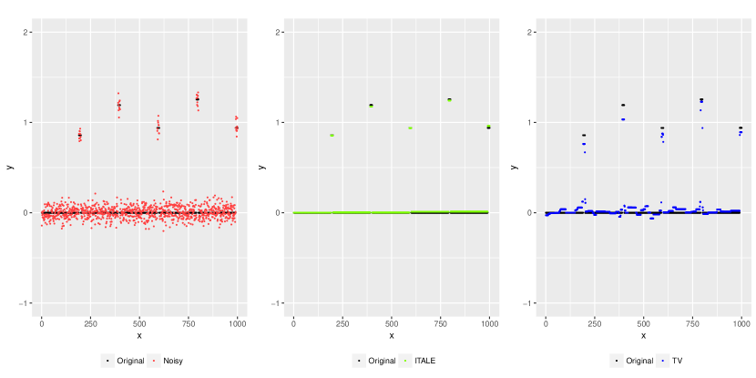
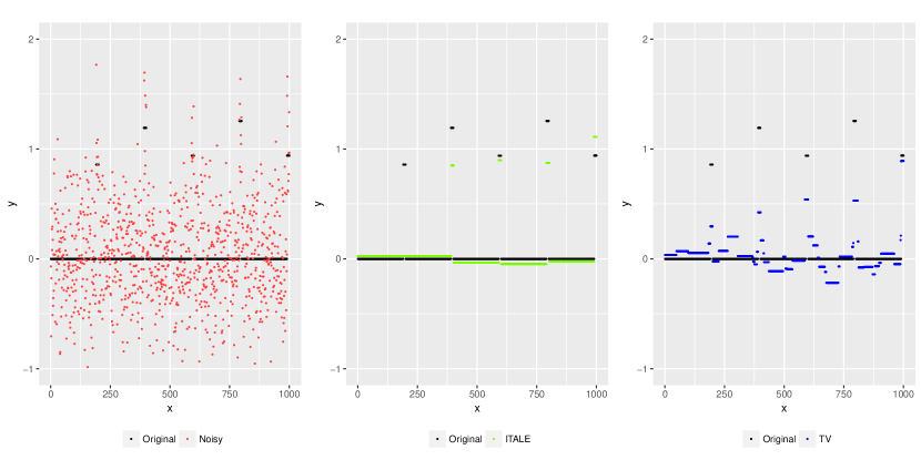
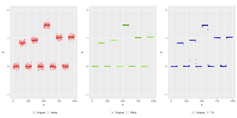
We tested ITALE on two simulated signals for the linear chain graph, with different changepoint structures: the “spike” signal depicted in Figures 3 and 3, and the “wave” signal depicted in Figure 5 and 5. The two signals both have vertices with break points. The spike signal consists of short segments of length 10 with elevated mean, while the breaks of the wave signal are equally-spaced.
We sampled random Gaussian measurements . The measurement error was generated as Gaussian noise . To provide an intuitive understanding of the tested signal-to-noise, we plot in red in Figures 3 to 5, corresponding to two different tested noise levels. Recall that ITALE denoises in each iteration (corresponding to for this normalization of ), so that represents the noisy signal in an ideal setting if is a perfect estimate from the preceding iteration.
Tables 1 and 2 display the root-mean-squared estimation errors
for undersampling ratio from 10% to 50%, and a range of noise levels that yielded RMSE values between 0 and roughly 0.2. Each reported error value is an average across 20 independent simulations. In these results, the iterate in ITALE and penalty parameter in TV were both selected using 5-fold cross-validation. Best-achieved errors over all and are reported in Appendix C, and suggest the same qualitative conclusions. Standard deviations of the RMSE across simulations are also reported in Appendix C.
In the spike example, ITALE yielded lower RMSE in all of the above settings of undersampling and signal-to-noise. Figures 3 and 3 display one instance each of the resulting estimates and at 15% undersampling, illustrating some of their differences and typical features. Under optimal tuning, returns an undersmoothed estimate even in a low-noise setting where ITALE can often correctly estimate the changepoint locations. With higher noise, ITALE begins to miss changepoints and oversmooth.
In the wave example, with undersampling ranging between 15% and 50%, ITALE yielded lower RMSE at most tested noise levels. Figures 5 and 5 depict two instances of the recovered signals at 15% undersampling. For 10% undersampling, the component of the effective noise was sufficiently high such that ITALE often did not estimate the true changepoint structure, and TV usually outperformed ITALE in this case. The standard deviations of RMSE reported in Appendix C indicate that the ITALE estimates are a bit more variable than the TV estimates in all tested settings, but particularly so in this 10% undersampling regime.
| 10% | ITALE | 0.000 | 0.014 | 0.060 | 0.090 | 0.144 | 0.173 | 0.199 | 0.216 |
|---|---|---|---|---|---|---|---|---|---|
| TV | 0.000 | 0.047 | 0.092 | 0.129 | 0.160 | 0.189 | 0.213 | 0.228 | |
| 15% | ITALE | 0.000 | 0.009 | 0.023 | 0.049 | 0.076 | 0.104 | 0.133 | 0.153 |
| TV | 0.000 | 0.030 | 0.060 | 0.088 | 0.114 | 0.136 | 0.158 | 0.175 | |
| 20% | ITALE | 0.000 | 0.007 | 0.015 | 0.032 | 0.056 | 0.076 | 0.099 | 0.123 |
| TV | 0.000 | 0.022 | 0.045 | 0.067 | 0.089 | 0.109 | 0.128 | 0.146 | |
| 30% | ITALE | 0.000 | 0.006 | 0.012 | 0.021 | 0.031 | 0.049 | 0.065 | 0.079 |
| TV | 0.000 | 0.017 | 0.035 | 0.052 | 0.070 | 0.087 | 0.104 | 0.120 | |
| 40% | ITALE | 0.000 | 0.005 | 0.010 | 0.015 | 0.025 | 0.041 | 0.051 | 0.063 |
| TV | 0.000 | 0.014 | 0.028 | 0.043 | 0.057 | 0.071 | 0.085 | 0.098 | |
| 50% | ITALE | 0.000 | 0.005 | 0.010 | 0.015 | 0.023 | 0.033 | 0.040 | 0.051 |
| TV | 0.000 | 0.013 | 0.026 | 0.038 | 0.051 | 0.064 | 0.075 | 0.088 |
| 10% | ITALE | 0.036 | 0.040 | 0.118 | 0.150 | 0.198 | 0.236 | 0.262 | 0.315 |
|---|---|---|---|---|---|---|---|---|---|
| TV | 0.000 | 0.032 | 0.064 | 0.093 | 0.120 | 0.143 | 0.168 | 0.189 | |
| 15% | ITALE | 0.000 | 0.009 | 0.025 | 0.059 | 0.090 | 0.111 | 0.143 | 0.176 |
| TV | 0.000 | 0.023 | 0.046 | 0.068 | 0.089 | 0.109 | 0.127 | 0.144 | |
| 20% | ITALE | 0.000 | 0.007 | 0.017 | 0.039 | 0.061 | 0.079 | 0.103 | 0.121 |
| TV | 0.000 | 0.019 | 0.037 | 0.056 | 0.074 | 0.092 | 0.108 | 0.124 | |
| 30% | ITALE | 0.000 | 0.006 | 0.012 | 0.019 | 0.035 | 0.051 | 0.065 | 0.085 |
| TV | 0.000 | 0.014 | 0.028 | 0.042 | 0.056 | 0.070 | 0.084 | 0.097 | |
| 40% | ITALE | 0.000 | 0.005 | 0.011 | 0.018 | 0.027 | 0.037 | 0.052 | 0.064 |
| TV | 0.000 | 0.012 | 0.024 | 0.037 | 0.049 | 0.061 | 0.073 | 0.085 | |
| 50% | ITALE | 0.000 | 0.005 | 0.010 | 0.016 | 0.024 | 0.033 | 0.044 | 0.055 |
| TV | 0.000 | 0.011 | 0.022 | 0.033 | 0.043 | 0.054 | 0.065 | 0.075 |
4.2. 2-D phantom images
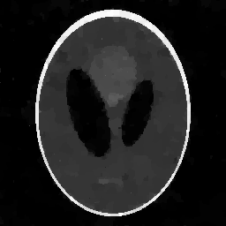
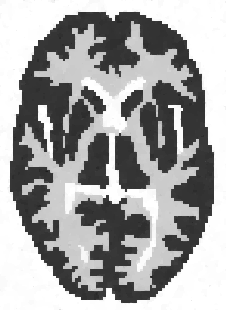
Next, we tested ITALE on three 2-D image examples, corresponding to piecewise-constant digital phantom images of varying complexity: the Shepp-Logan digital phantom depicted in Figure 6, a digital brain phantom from [FH94] depicted in Figure 7, and the XCAT chest slice from [GHG+17] as previously depicted in Figure 1.
| 10% | ITALE | 0.001 | 0.007 | 0.012 | 0.018 | 0.023 | 0.039 | 0.047 | 0.072 |
|---|---|---|---|---|---|---|---|---|---|
| TV | 0.005 | 0.011 | 0.021 | 0.031 | 0.040 | 0.051 | 0.057 | 0.062 | |
| 15% | ITALE | 0.000 | 0.003 | 0.011 | 0.014 | 0.017 | 0.027 | 0.035 | 0.044 |
| TV | 0.001 | 0.008 | 0.016 | 0.026 | 0.030 | 0.038 | 0.049 | 0.053 | |
| 20% | ITALE | 0.000 | 0.003 | 0.008 | 0.012 | 0.017 | 0.024 | 0.027 | 0.036 |
| TV | 0.000 | 0.007 | 0.014 | 0.021 | 0.027 | 0.032 | 0.039 | 0.045 | |
| 30% | ITALE | 0.000 | 0.002 | 0.005 | 0.011 | 0.013 | 0.015 | 0.018 | 0.026 |
| TV | 0.000 | 0.006 | 0.012 | 0.017 | 0.023 | 0.027 | 0.032 | 0.036 | |
| 40% | ITALE | 0.000 | 0.001 | 0.005 | 0.010 | 0.011 | 0.013 | 0.017 | 0.018 |
| TV | 0.000 | 0.005 | 0.010 | 0.015 | 0.019 | 0.023 | 0.028 | 0.032 | |
| 50% | ITALE | 0.000 | 0.001 | 0.004 | 0.008 | 0.011 | 0.013 | 0.013 | 0.015 |
| TV | 0.000 | 0.005 | 0.009 | 0.013 | 0.017 | 0.021 | 0.025 | 0.029 |
| 10% | ITALE | 0.003 | 0.002 | 0.010 | 0.028 | 0.043 | 0.060 | 0.080 | 0.096 |
|---|---|---|---|---|---|---|---|---|---|
| TV | 0.002 | 0.014 | 0.028 | 0.042 | 0.054 | 0.064 | 0.078 | 0.085 | |
| 15% | ITALE | 0.000 | 0.001 | 0.007 | 0.019 | 0.030 | 0.044 | 0.059 | 0.075 |
| TV | 0.001 | 0.011 | 0.022 | 0.032 | 0.043 | 0.053 | 0.063 | 0.074 | |
| 20% | ITALE | 0.000 | 0.001 | 0.005 | 0.012 | 0.025 | 0.036 | 0.047 | 0.056 |
| TV | 0.000 | 0.009 | 0.019 | 0.028 | 0.038 | 0.046 | 0.056 | 0.061 | |
| 30% | ITALE | 0.000 | 0.001 | 0.002 | 0.007 | 0.014 | 0.025 | 0.033 | 0.044 |
| TV | 0.000 | 0.007 | 0.016 | 0.023 | 0.030 | 0.038 | 0.046 | 0.053 | |
| 40% | ITALE | 0.000 | 0.000 | 0.002 | 0.006 | 0.010 | 0.021 | 0.027 | 0.037 |
| TV | 0.000 | 0.007 | 0.013 | 0.019 | 0.026 | 0.032 | 0.039 | 0.043 | |
| 50% | ITALE | 0.000 | 0.001 | 0.002 | 0.005 | 0.007 | 0.016 | 0.022 | 0.029 |
| TV | 0.000 | 0.006 | 0.011 | 0.018 | 0.023 | 0.029 | 0.036 | 0.040 |
| 10% | ITALE | 0.063 | 0.064 | 0.068 | 0.078 | 0.084 | 0.092 | 0.099 | 0.106 |
|---|---|---|---|---|---|---|---|---|---|
| TV | 0.009 | 0.019 | 0.032 | 0.044 | 0.054 | 0.061 | 0.068 | 0.072 | |
| 15% | ITALE | 0.002 | 0.007 | 0.025 | 0.036 | 0.048 | 0.070 | 0.079 | 0.085 |
| TV | 0.005 | 0.014 | 0.024 | 0.035 | 0.043 | 0.050 | 0.056 | 0.061 | |
| 20% | ITALE | 0.002 | 0.005 | 0.014 | 0.023 | 0.033 | 0.045 | 0.052 | 0.079 |
| TV | 0.002 | 0.011 | 0.020 | 0.028 | 0.037 | 0.043 | 0.049 | 0.056 | |
| 30% | ITALE | 0.002 | 0.004 | 0.011 | 0.018 | 0.025 | 0.033 | 0.041 | 0.049 |
| TV | 0.002 | 0.008 | 0.016 | 0.023 | 0.030 | 0.036 | 0.042 | 0.046 | |
| 40% | ITALE | 0.002 | 0.003 | 0.009 | 0.014 | 0.020 | 0.026 | 0.033 | 0.038 |
| TV | 0.001 | 0.007 | 0.014 | 0.020 | 0.025 | 0.031 | 0.036 | 0.041 | |
| 50% | ITALE | 0.002 | 0.003 | 0.008 | 0.013 | 0.018 | 0.024 | 0.029 | 0.033 |
| TV | 0.001 | 0.006 | 0.012 | 0.018 | 0.024 | 0.029 | 0.033 | 0.038 |
Each image was normalized to have pixel value in . We sampled random Fourier design matrices as specified in (11), fixing the constant in the weight distribution (10) for this design. This yielded the best recovery across several tested values for both ITALE and TV. The measurement error was generated as Gaussian noise , applied to the measurements before the normalization. Tables 3, 4, and 5 display the RMSE of the estimates and for a single simulation, with tuning parameters selected by 5-fold cross-validation. Best-achieved errors are reported in Appendix C.
For the simpler Logan-Shepp and brain phantom images, which exhibit stronger gradient-sparsity, ITALE yielded lower RMSE in nearly all tested undersampling and signal-to-noise regimes. For the XCAT chest phantom, with undersampling ranging between 15% and 50%, ITALE yielded lower RMSE at a range of tested noise levels, and in particular for those settings of higher signal-to-noise. With 10% undersampling for the XCAT phantom, ITALE was not able to recover some details of the XCAT image even with no measurement noise, and RMSE was higher than TV at all tested noise levels. Results of Appendix C indicate that this is partially due to sub-optimal selection of the tuning parameter using 5-fold cross-validation, caused by the further reduction of undersampling from 10% to 8% in the size of the training data in each fold.


Examples of recovered signals and are depicted for the Shepp-Logan and brain phantoms in Figures 6 and 7, at 15% and 20% undersampling for two low-noise and medium-noise settings. The qualitative comparisons are similar to those in the 1-D simulations, and to those previously depicted for the XCAT chest slice in Figure 1: As measurement noise increases, ITALE begins to lose finer details, while TV begins to yield an undersmoothed and blotchy image. These observations are also similar to previous comparisons that have been made for algorithms oriented towards versus TV regularization for direct measurements , in [XLXJ11, FG18, KG19].
5. Conclusion
We have studied recovery of piecewise-constant signals over arbitrary graphs from noisy linear measurements. We have proposed an iterative algorithm, ITALE, to minimize an -edge-penalized least-squares objective. Under a cut-restricted isometry property for the measurement design, we have established global recovery guarantees for the estimated signal, in noisy and noiseless settings.
In the field of compressed sensing, for signals exhibiting sparsity in an orthonormal basis, -regularization [Don06, CRT06b, CRT06a] and discrete iterative algorithms [TG07, NT09, BD09] constitute two major approaches for signal recovery. It has been observed that for recovering piecewise-constant signals, regularizing the signal gradient in a sparse analysis framework can yield better empirical recovery than regularizing signal coefficients in such a basis. Whereas -regularization extends naturally to the sparse analysis setting, iterative algorithms have received less attention. By applying the alpha-expansion idea for MAP estimation in discrete Markov random fields, ITALE provides a computationally tractable approach for “iterative thresholding” recovery of gradient-sparse signals, with provable recovery guarantees.
In contrast to sparse signal recovery over an orthonormal basis, the comparison of versus regularization for gradient-based sparsity is graph-dependent. Using an -based approach, we establish signal recovery guarantees on the 1-D and 2-D lattice graphs with numbers of measurements optimal up to a constant factor, which were not previously available for TV-regularization. This difference is closely connected to slow and fast rates of convergence for lasso and best-subset regression for correlated regression designs [BRvdGZ13, ZWJ14, DHL17]. ITALE provides a polynomial-time approach for -regularization in a special graph-based setting, and we believe it is an interesting question whether similar algorithmic ideas may be applicable to other classes of sparse regression problems.
Appendix A Proof of robust recovery guarantee
In this appendix, we prove Theorem 3.5 providing the estimation guarantee under approximate gradient-sparsity and discretization and measurement error.
Lemma A.1.
Suppose has maximum vertex degree , and satisfies -cRIP. Then for any and ,
Proof.
Let be the indices corresponding to the entries of with largest magnitude (breaking ties arbitrarily). Let be the indices corresponding to the next entries of with largest magnitude, and define sequentially for in this way. Denote by the vector with entry equal to if , or 0 otherwise. Then for each . Applying the triangle inequality and cRIP condition for ,
For , we have by construction, so
Applying this for , and the bound for ,
Finally, we have by the concavity of , and hence since . ∎
Proof of Theorem 3.5.
Write where . Denote
As in the proof of Theorem 3.4, consider the partitions of induced by the piecewise-constant structures of , , and , let be their common refinement, and let be the orthogonal projection onto the subspace of signals taking constant value over each set in . Applying
the same arguments as leading to (15) yield
| (22) |
Set , , and
Then we obtain analogously to (16) and (19) that
and hence
| (23) |
Similarly, taking the square-root in (22), we obtain analogously to (20) that
| (24) |
Recalling the bound from (17), we have
Bounding using the given cRIP condition and Lemma A.1 with the choice as above, we get for a constant that
Applying this and the bound from (18) to (23), we get
| (25) |
for the quantity
Also, applying this to (24), we get
| (26) |
We now claim by induction on that if and for every , where is sufficiently large and is sufficiently small, then for every we have
| (27) |
For , these are satisfied as and . Assume inductively that these hold for , where . Then for small enough , we have and hence
Also, for a constant independent of . Then for large enough and small enough, we obtain from (25) and the condition that
This gives the bound
Appendix B Proofs of cut-restricted isometry property
In this appendix, we prove Propositions 3.2 and 3.3 establishing cRIP for the sub-Gaussian and weighted 2D-Fourier designs.
Proof of Proposition 3.2.
First fix . For each partition of with , let be the associated orthogonal projection onto the subspace of signals which are constant on each set in . Note that the dimension of is the number of sets in , which is at most because is a connected graph. Write , where has orthonormal columns spanning . Then still has independent rows , where and . Applying [Ver10, Eq. (5.25)] to , for any and some constants depending only on ,
Let , and note that there are at most partitions where . Taking a union bound over , and noting that any with may be represented as for some such , this yields
When and , we have
We also have
where the last inequality is trivial for and may be checked for by squaring both sides and applying in this case. Then, for any and some constants depending on , setting and applying , we get
Taking a union bound over and applying scale invariance of the cRIP condition to concludes the proof. ∎
Next, we establish Proposition 3.3 on the Fourier design.
Lemma B.1.
Let , let be any connected rectangle, and let be the 2-D discrete Fourier matrix defined in Section 3.1. Then for any ,
Proof.
Since
for the 1-D Fourier matrices and , it suffices to show
For this, denote the elements of as , and write
This is at most , which implies the bound for . For , apply further
for . Then summing the geometric series, we also have
The result follows from combining this with the previous upper bound bound , using . ∎
Lemma B.2.
Let , where are powers of 2 and for a constant . Let be the 2-D lattice graph of size . For , let be the ordered magnitudes of the coefficients of in the bivariate Haar wavelet basis. If is centered to have mean entry 0, then for a constant and each ,
where is the discrete gradient operator on .
Proof.
See [NW13b, Proposition 8] for the case . For , we may apply this result to the “stretched” image where each original vertex value is copied to consecutive values in a vertical strip. This stretching changes and each original bivariate Haar wavelet coefficient by at most a constant factor, and introduces new Haar wavelet coefficients which are identically 0. Thus the result still holds in this case, and similarly for . ∎
Proof of Proposition 3.3.
We follow closely the ideas of [RV08, Theorem 3.3].
For each partition of into connected pieces, let be the -dimensional subspace of vectors which take a constant value over each set of . For each sparsity level , define
It suffices to show, with the stated probability and form of , that
holds simultaneously for all .
We first control using a metric entropy argument: Letting be row of ,
So
Applying Gaussian symmetrization,
for a constant and independent of .
Condition on , and define by the right side above with the expectation taken only over . Introducing the pseudo-metric
Dudley’s inequality yields
where is the covering number of by balls of radius in the metric . For ,
where
Applying this bound and a change-of-variables ,
| (28) |
The pseudo-norm has the following property: For any ,
| (29) |
where the middle inequality applies and the fact that the maximal vertex degree in is 4. Let be the bivariate Haar wavelet basis, and write the orthogonal decomposition . Then, as , , and , Lemma B.2 implies
| (30) |
Each Haar vector is supported on a number of rectangular pieces of some size , with a constant value on each piece. Then Lemma B.1 implies for each
From the definition of and the bound ,
for a constant . Then from the definitions of and , the bound (30), and the condition , we obtain
| (31) |
As in [RV08, Theorem 3.3], we bound the covering number in two ways: First, fix any and write now its Haar decomposition as
where . Then for some universal constant , we obtain from (30)
Applying Maurey’s argument, define a discrete distribution over a random vector by
Then by construction, . Letting be independent copies of , for a value to be chosen later, Gaussian symmetrization yields (with all expectations conditional on )
| (32) |
for . The bound (31) yields for every
Applying this to (32) with a Gaussian tail bound and union bound,
For any , choosing ensures this bound is at most . Then by the probabilistic method, belongs to the -ball of radius around some vector of the form . The support of the distribution of has cardinality at most , and this support is the same for all . Then there are at most such vectors, so we obtain
| (33) |
We obtain a second covering bound by a union bound over : For any with , note that . Define such that its th column is where is the indicator of . Then is the projection onto , and
As by (31), a standard volume argument yields for
The number of partitions with is at most . Applying and summing over ,
| (34) |
Returning to the entropy integral in (28), note that (31) implies for , so the integral may be restricted to . Setting , applying (34) for , and also applying Cauchy-Schwarz and , we get
Applying (33) for , we get
Applying these bounds to (28) gives
Taking now the expectation over and applying Cauchy-Schwarz and the triangle inequality,
This yields
We now show concentration of each quantity around its mean. The argument is similar to [RV08, Theorem 3.9], and we omit some details. Write
where . Let be an independent copy of and define
Then by the same arguments as [RV08, Theorem 3.9], for any ,
| (35) |
From (31), we have
for every . Then applying [RV08, Theorem 3.8], for any integers , any , and some constants ,
Let us assume without loss of generality and set , , and , where denotes the integer part. Then combining this with (35), we get for some constants and all that
Setting for a sufficiently large constant , this yields
The result follows from taking a union bound over , and noting and
for all and sufficiently large . ∎
Appendix C RMSE for optimal parameter tuning
We report here the best-achieved RMSE, rather than RMSE for cross-validated selection of tuning parameters, corresponding to Tables 1, 2, 3, 4, and 5. For the 1-D signals, we performed 20 independent simulations, and we report also the standard deviations across these 20 simulations.
| 10% | ITALE | 0.000 | 0.011 | 0.050 | 0.081 | 0.115 | 0.138 | 0.177 | 0.198 |
|---|---|---|---|---|---|---|---|---|---|
| (0.000) | (0.004) | (0.024) | (0.023) | (0.033) | (0.034) | (0.031) | (0.025) | ||
| TV | 0.000 | 0.045 | 0.086 | 0.122 | 0.152 | 0.176 | 0.193 | 0.206 | |
| (0.000) | (0.011) | (0.017) | (0.018) | (0.017) | (0.016) | (0.017) | (0.015) | ||
| 15% | ITALE | 0.000 | 0.008 | 0.019 | 0.042 | 0.069 | 0.091 | 0.114 | 0.133 |
| (0.000) | (0.002) | (0.007) | (0.016) | (0.023) | (0.029) | (0.028) | (0.029) | ||
| TV | 0.000 | 0.029 | 0.057 | 0.085 | 0.109 | 0.130 | 0.149 | 0.165 | |
| (0.000) | (0.006) | (0.011) | (0.016) | (0.020) | (0.020) | (0.020) | (0.020) | ||
| 20% | ITALE | 0.000 | 0.007 | 0.013 | 0.028 | 0.049 | 0.070 | 0.090 | 0.102 |
| (0.000) | (0.002) | (0.003) | (0.012) | (0.019) | (0.019) | (0.017) | (0.020) | ||
| TV | 0.000 | 0.022 | 0.044 | 0.066 | 0.087 | 0.107 | 0.126 | 0.143 | |
| (0.000) | (0.002) | (0.004) | (0.006) | (0.008) | (0.009) | (0.010) | (0.010) | ||
| 30% | ITALE | 0.000 | 0.006 | 0.012 | 0.019 | 0.029 | 0.045 | 0.061 | 0.075 |
| (0.000) | (0.001) | (0.003) | (0.006) | (0.009) | (0.014) | (0.011) | (0.013) | ||
| TV | 0.000 | 0.017 | 0.034 | 0.051 | 0.068 | 0.085 | 0.101 | 0.116 | |
| (0.000) | (0.001) | (0.003) | (0.004) | (0.006) | (0.007) | (0.008) | (0.009) | ||
| 40% | ITALE | 0.000 | 0.005 | 0.010 | 0.015 | 0.024 | 0.038 | 0.048 | 0.062 |
| (0.000) | (0.001) | (0.002) | (0.003) | (0.007) | (0.012) | (0.015) | (0.016) | ||
| TV | 0.000 | 0.014 | 0.028 | 0.042 | 0.056 | 0.070 | 0.084 | 0.097 | |
| (0.000) | (0.001) | (0.003) | (0.004) | (0.006) | (0.007) | (0.008) | (0.010) | ||
| 50% | ITALE | 0.000 | 0.005 | 0.009 | 0.014 | 0.021 | 0.029 | 0.036 | 0.047 |
| (0.000) | (0.001) | (0.002) | (0.003) | (0.006) | (0.011) | (0.013) | (0.013) | ||
| TV | 0.000 | 0.013 | 0.025 | 0.038 | 0.050 | 0.063 | 0.074 | 0.086 | |
| (0.000) | (0.002) | (0.003) | (0.005) | (0.006) | (0.008) | (0.008) | (0.009) |
| 10% | ITALE | 0.019 | 0.030 | 0.075 | 0.126 | 0.155 | 0.203 | 0.233 | 0.256 |
|---|---|---|---|---|---|---|---|---|---|
| (0.081) | (0.066) | (0.055) | (0.057) | (0.064) | (0.059) | (0.070) | (0.068) | ||
| TV | 0.000 | 0.031 | 0.062 | 0.090 | 0.114 | 0.137 | 0.157 | 0.176 | |
| (0.000) | (0.005) | (0.011) | (0.016) | (0.018) | (0.021) | (0.022) | (0.024) | ||
| 15% | ITALE | 0.000 | 0.008 | 0.022 | 0.052 | 0.083 | 0.105 | 0.134 | 0.154 |
| (0.000) | (0.002) | (0.011) | (0.023) | (0.027) | (0.030) | (0.027) | (0.035) | ||
| TV | 0.000 | 0.022 | 0.044 | 0.066 | 0.087 | 0.106 | 0.124 | 0.141 | |
| (0.000) | (0.003) | (0.006) | (0.009) | (0.011) | (0.013) | (0.014) | (0.016) | ||
| 20% | ITALE | 0.000 | 0.006 | 0.015 | 0.032 | 0.050 | 0.072 | 0.093 | 0.109 |
| (0.000) | (0.001) | (0.006) | (0.011) | (0.016) | (0.023) | (0.027) | (0.027) | ||
| TV | 0.000 | 0.018 | 0.036 | 0.054 | 0.071 | 0.088 | 0.104 | 0.118 | |
| (0.000) | (0.002) | (0.004) | (0.007) | (0.009) | (0.011) | (0.012) | (0.013) | ||
| 30% | ITALE | 0.000 | 0.006 | 0.011 | 0.017 | 0.032 | 0.046 | 0.062 | 0.077 |
| (0.000) | (0.001) | (0.002) | (0.004) | (0.010) | (0.012) | (0.015) | (0.015) | ||
| TV | 0.000 | 0.014 | 0.027 | 0.041 | 0.055 | 0.068 | 0.082 | 0.095 | |
| (0.000) | (0.001) | (0.003) | (0.004) | (0.005) | (0.007) | (0.008) | (0.010) | ||
| 40% | ITALE | 0.000 | 0.005 | 0.010 | 0.016 | 0.024 | 0.033 | 0.046 | 0.057 |
| (0.000) | (0.001) | (0.002) | (0.004) | (0.009) | (0.012) | (0.014) | (0.017) | ||
| TV | 0.000 | 0.012 | 0.024 | 0.036 | 0.048 | 0.060 | 0.072 | 0.083 | |
| (0.000) | (0.001) | (0.002) | (0.003) | (0.005) | (0.006) | (0.007) | (0.008) | ||
| 50% | ITALE | 0.000 | 0.004 | 0.009 | 0.015 | 0.022 | 0.030 | 0.038 | 0.049 |
| (0.000) | (0.001) | (0.002) | (0.005) | (0.009) | (0.011) | (0.012) | (0.018) | ||
| TV | 0.000 | 0.011 | 0.021 | 0.032 | 0.042 | 0.053 | 0.063 | 0.073 | |
| (0.000) | (0.001) | (0.003) | (0.004) | (0.005) | (0.007) | (0.008) | (0.009) |
| 10% | ITALE | 0.000 | 0.004 | 0.012 | 0.016 | 0.023 | 0.037 | 0.046 | 0.067 |
|---|---|---|---|---|---|---|---|---|---|
| TV | 0.002 | 0.011 | 0.021 | 0.030 | 0.038 | 0.049 | 0.056 | 0.061 | |
| 15% | ITALE | 0.000 | 0.003 | 0.010 | 0.013 | 0.017 | 0.025 | 0.035 | 0.044 |
| TV | 0.001 | 0.008 | 0.016 | 0.025 | 0.030 | 0.038 | 0.047 | 0.052 | |
| 20% | ITALE | 0.000 | 0.003 | 0.008 | 0.011 | 0.016 | 0.018 | 0.026 | 0.035 |
| TV | 0.001 | 0.007 | 0.014 | 0.021 | 0.027 | 0.032 | 0.039 | 0.045 | |
| 30% | ITALE | 0.000 | 0.002 | 0.005 | 0.011 | 0.013 | 0.015 | 0.018 | 0.023 |
| TV | 0.002 | 0.006 | 0.011 | 0.017 | 0.022 | 0.027 | 0.032 | 0.036 | |
| 40% | ITALE | 0.000 | 0.001 | 0.005 | 0.009 | 0.011 | 0.013 | 0.016 | 0.018 |
| TV | 0.001 | 0.005 | 0.010 | 0.014 | 0.019 | 0.023 | 0.026 | 0.031 | |
| 50% | ITALE | 0.000 | 0.001 | 0.004 | 0.008 | 0.010 | 0.012 | 0.013 | 0.015 |
| TV | 0.001 | 0.005 | 0.009 | 0.013 | 0.017 | 0.021 | 0.025 | 0.029 |
| 10% | ITALE | 0.000 | 0.002 | 0.010 | 0.028 | 0.042 | 0.058 | 0.077 | 0.093 |
|---|---|---|---|---|---|---|---|---|---|
| TV | 0.002 | 0.014 | 0.028 | 0.041 | 0.054 | 0.064 | 0.077 | 0.085 | |
| 15% | ITALE | 0.000 | 0.001 | 0.007 | 0.017 | 0.030 | 0.043 | 0.057 | 0.075 |
| TV | 0.001 | 0.011 | 0.022 | 0.032 | 0.043 | 0.053 | 0.063 | 0.071 | |
| 20% | ITALE | 0.000 | 0.001 | 0.005 | 0.012 | 0.025 | 0.034 | 0.047 | 0.054 |
| TV | 0.001 | 0.009 | 0.019 | 0.028 | 0.037 | 0.044 | 0.055 | 0.061 | |
| 30% | ITALE | 0.000 | 0.001 | 0.002 | 0.007 | 0.014 | 0.024 | 0.033 | 0.043 |
| TV | 0.001 | 0.007 | 0.016 | 0.022 | 0.030 | 0.038 | 0.044 | 0.052 | |
| 40% | ITALE | 0.000 | 0.000 | 0.002 | 0.005 | 0.010 | 0.018 | 0.026 | 0.032 |
| TV | 0.001 | 0.007 | 0.013 | 0.019 | 0.026 | 0.032 | 0.039 | 0.043 | |
| 50% | ITALE | 0.000 | 0.001 | 0.002 | 0.004 | 0.007 | 0.012 | 0.019 | 0.027 |
| TV | 0.001 | 0.006 | 0.011 | 0.017 | 0.023 | 0.029 | 0.034 | 0.040 |
| 10% | ITALE | 0.002 | 0.032 | 0.043 | 0.068 | 0.075 | 0.084 | 0.093 | 0.101 |
|---|---|---|---|---|---|---|---|---|---|
| TV | 0.006 | 0.019 | 0.032 | 0.044 | 0.053 | 0.061 | 0.068 | 0.072 | |
| 15% | ITALE | 0.002 | 0.007 | 0.017 | 0.029 | 0.044 | 0.067 | 0.076 | 0.084 |
| TV | 0.003 | 0.014 | 0.024 | 0.034 | 0.043 | 0.050 | 0.056 | 0.061 | |
| 20% | ITALE | 0.002 | 0.005 | 0.014 | 0.022 | 0.032 | 0.041 | 0.052 | 0.069 |
| TV | 0.002 | 0.011 | 0.020 | 0.028 | 0.037 | 0.043 | 0.049 | 0.056 | |
| 30% | ITALE | 0.002 | 0.004 | 0.011 | 0.017 | 0.024 | 0.030 | 0.038 | 0.049 |
| TV | 0.002 | 0.008 | 0.016 | 0.023 | 0.029 | 0.035 | 0.041 | 0.046 | |
| 40% | ITALE | 0.002 | 0.003 | 0.008 | 0.014 | 0.020 | 0.026 | 0.032 | 0.038 |
| TV | 0.001 | 0.007 | 0.014 | 0.020 | 0.025 | 0.031 | 0.036 | 0.041 | |
| 50% | ITALE | 0.001 | 0.003 | 0.007 | 0.013 | 0.017 | 0.023 | 0.028 | 0.033 |
| TV | 0.001 | 0.006 | 0.012 | 0.018 | 0.023 | 0.028 | 0.033 | 0.038 |
References
- [BD09] Thomas Blumensath and Mike E Davies. Iterative hard thresholding for compressed sensing. Applied and Computational Harmonic Analysis, 27(3):265–274, 2009.
- [BK04] Yuri Boykov and Vladimir Kolmogorov. An experimental comparison of min-cut/max-flow algorithms for energy minimization in vision. IEEE Transactions on Pattern Analysis & Machine Intelligence, 9:1124–1137, 2004.
- [BKM16] Dimitris Bertsimas, Angela King, and Rahul Mazumder. Best subset selection via a modern optimization lens. The Annals of Statistics, 44(2):813–852, 2016.
- [BRvdGZ13] Peter Bühlmann, Philipp Rütimann, Sara van de Geer, and Cun-Hui Zhang. Correlated variables in regression: clustering and sparse estimation. Journal of Statistical Planning and Inference, 143(11):1835–1858, 2013.
- [BT09] Amir Beck and Marc Teboulle. A fast iterative shrinkage-thresholding algorithm for linear inverse problems. SIAM Journal on Imaging Sciences, 2(1):183–202, 2009.
- [BVZ99] Yuri Boykov, Olga Veksler, and Ramin Zabih. Fast approximate energy minimization via graph cuts. In Proceedings of the Seventh IEEE International Conference on Computer Vision, volume 1, pages 377–384. IEEE, 1999.
- [CENR11] Emmanuel J Candès, Yonina C Eldar, Deanna Needell, and Paige Randall. Compressed sensing with coherent and redundant dictionaries. Applied and Computational Harmonic Analysis, 31(1):59–73, 2011.
- [CRT06a] Emmanuel J Candès, Justin Romberg, and Terence Tao. Robust uncertainty principles: Exact signal reconstruction from highly incomplete frequency information. IEEE Transactions on Information Theory, 52(2):489, 2006.
- [CRT06b] Emmanuel J Candès, Justin K Romberg, and Terence Tao. Stable signal recovery from incomplete and inaccurate measurements. Communications on Pure and Applied Mathematics, 59(8):1207–1223, 2006.
- [CX15] Jian-Feng Cai and Weiyu Xu. Guarantees of total variation minimization for signal recovery. Information and Inference: A Journal of the IMA, 4(4):328–353, 2015.
- [DHL17] Arnak S Dalalyan, Mohamed Hebiri, and Johannes Lederer. On the prediction performance of the Lasso. Bernoulli, 23(1):552–581, 2017.
- [Don06] David L Donoho. Compressed sensing. IEEE Transactions on Information Theory, 52(4):1289–1306, 2006.
- [EKDN18] Ethan R Elenberg, Rajiv Khanna, Alexandros G Dimakis, and Sahand Negahban. Restricted strong convexity implies weak submodularity. The Annals of Statistics, 46(6B):3539–3568, 2018.
- [EMR07] Michael Elad, Peyman Milanfar, and Ron Rubinstein. Analysis versus synthesis in signal priors. Inverse Problems, 23(3):947, 2007.
- [FG18] Zhou Fan and Leying Guan. Approximate -penalized estimation of piecewise-constant signals on graphs. The Annals of Statistics, 46(6B):3217–3245, 2018.
- [FH94] Jeffrey A Fessler and Alfred O Hero. Space-alternating generalized EM algorithms for penalized maximum-likelihood image reconstruction. Technical report, Technical Report 286, Comm. and Sign. Proc. Lab., Dept. of EECS, Univ. of …, 1994.
- [GHG+17] Changfei Gong, Ce Han, Guanghui Gan, Zhenxiang Deng, Yongqiang Zhou, Jinling Yi, Xiaomin Zheng, Congying Xie, and Xiance Jin. Low-dose dynamic myocardial perfusion CT image reconstruction using pre-contrast normal-dose CT scan induced structure tensor total variation regularization. Physics in Medicine & Biology, 62(7):2612, 2017.
- [HR16] Jan-Christian Hütter and Philippe Rigollet. Optimal rates for total variation denoising. In Conference on Learning Theory, pages 1115–1146, 2016.
- [KG19] Youngseok Kim and Chao Gao. Bayesian model selection with graph structured sparsity. arXiv preprint arXiv:1902.03316, 2019.
- [KKBG09] Seung-Jean Kim, Kwangmoo Koh, Stephen Boyd, and Dimitry Gorinevsky. trend filtering. SIAM review, 51(2):339–360, 2009.
- [KT02] Jon Kleinberg and Eva Tardos. Approximation algorithms for classification problems with pairwise relationships: Metric labeling and markov random fields. Journal of the ACM (JACM), 49(5):616–639, 2002.
- [KW14] Felix Krahmer and Rachel Ward. Stable and robust sampling strategies for compressive imaging. IEEE Transactions on Image Processing, 23(2):612–622, 2014.
- [LDP07] Michael Lustig, David Donoho, and John M Pauly. Sparse MRI: The application of compressed sensing for rapid MR imaging. Magnetic Resonance in Medicine: An Official Journal of the International Society for Magnetic Resonance in Medicine, 58(6):1182–1195, 2007.
- [LMRW18] Yuan Li, Benjamin Mark, Garvesh Raskutti, and Rebecca Willett. Graph-based regularization for regression problems with highly-correlated designs. In 2018 IEEE Global Conference on Signal and Information Processing (GlobalSIP), pages 740–742. IEEE, 2018.
- [NDEG13] Sangnam Nam, Mike E Davies, Michael Elad, and Rémi Gribonval. The cosparse analysis model and algorithms. Applied and Computational Harmonic Analysis, 34(1):30–56, 2013.
- [NT09] Deanna Needell and Joel A Tropp. CoSaMP: Iterative signal recovery from incomplete and inaccurate samples. Applied and Computational Harmonic Analysis, 26(3):301–321, 2009.
- [NW13a] Deanna Needell and Rachel Ward. Near-optimal compressed sensing guarantees for total variation minimization. IEEE Transactions on Image Processing, 22(10):3941–3949, 2013.
- [NW13b] Deanna Needell and Rachel Ward. Stable image reconstruction using total variation minimization. SIAM Journal on Imaging Sciences, 6(2):1035–1058, 2013.
- [PB14] Neal Parikh and Stephen Boyd. Proximal algorithms. Foundations and Trends® in Optimization, 1(3):127–239, 2014.
- [Rin09] Alessandro Rinaldo. Properties and refinements of the fused lasso. The Annals of Statistics, 37(5B):2922–2952, 2009.
- [ROF92] Leonid I Rudin, Stanley Osher, and Emad Fatemi. Nonlinear total variation based noise removal algorithms. Physica D: Nonlinear Phenomena, 60(1-4):259–268, 1992.
- [RV08] Mark Rudelson and Roman Vershynin. On sparse reconstruction from Fourier and Gaussian measurements. Communications on Pure and Applied Mathematics, 61(8):1025–1045, 2008.
- [SSM+10] WP Segars, G Sturgeon, S Mendonca, Jason Grimes, and Benjamin MW Tsui. 4D XCAT phantom for multimodality imaging research. Medical Physics, 37(9):4902–4915, 2010.
- [TG07] Joel A Tropp and Anna C Gilbert. Signal recovery from random measurements via orthogonal matching pursuit. IEEE Transactions on Information Theory, 53(12):4655–4666, 2007.
- [Tib11] Ryan Joseph Tibshirani. The solution path of the generalized lasso. PhD thesis, Stanford University, 2011.
- [TSR+05] Robert Tibshirani, Michael Saunders, Saharon Rosset, Ji Zhu, and Keith Knight. Sparsity and smoothness via the fused lasso. Journal of the Royal Statistical Society: Series B (Statistical Methodology), 67(1):91–108, 2005.
- [Ver10] Roman Vershynin. Introduction to the non-asymptotic analysis of random matrices. arXiv preprint arXiv:1011.3027, 2010.
- [WSST16] Yu-Xiang Wang, James Sharpnack, Alexander J Smola, and Ryan J Tibshirani. Trend filtering on graphs. The Journal of Machine Learning Research, 17(1):3651–3691, 2016.
- [XLXJ11] Li Xu, Cewu Lu, Yi Xu, and Jiaya Jia. Image smoothing via gradient minimization. ACM Transactions on Graphics (TOG), 30(6):174, 2011.
- [Zha11] Tong Zhang. Sparse recovery with orthogonal matching pursuit under RIP. IEEE Transactions on Information Theory, 57(9):6215–6221, 2011.
- [ZWJ14] Yuchen Zhang, Martin J Wainwright, and Michael I Jordan. Lower bounds on the performance of polynomial-time algorithms for sparse linear regression. In Conference on Learning Theory, pages 921–948, 2014.