Mechanisms of astrophysical jet formation, and comparison with laboratory experiments

Abstract:

Jets are observed in young stellar objects, X-ray sources, active galactic nuclei (AGN). The mechanisms of jet formation may be divided in regular, acting continuously for a long time, and explosive ones [1]. Continuous mechanisms are related with electrodynamics and radiation pressure acceleration, hydrodynamical acceleration in the nozzle inside a thick disk, acceleration by relativistic beam of particles. Explosive jet formation is connected with supernovae, gamma ray bursts and explosive events in galactic nuclei. Mechanisms of jet collimation may be connected with magnetic confinement, or a pressure of external gas [2-4]. Explosive formation of jets in the laboratory is modeled in the experiments with powerful laser beam, and plasma focus [5,6].

1 Introduction

First model of AGN & quasar, as a supermassive black hole, surrounded by accretion disk, was suggested by D. Lynden-Bell [7] in the year 1969. This model was supported by observations, and now it is widely accepted that quasars and AGN nuclei contain supermassive black holes (SMBH). About 10 HMXR (high stellar mass black holes) are found in the Galaxy. They show behaviour, which, after appropriate scaling, is similar to the AGN SMBH, and were called as microquasars [8].

Jets are observed in objects with black holes, where collimated ejection from accretion disks is expected. Non-relativistic jets are observed in young stellar-like objects. AGN jets have been studied in many wavebands of the electromagnetic spectrum. The jet in the Virgo A galaxy M87 was observed in radio (14GHz, VLA) with angular resolution $\sim 0".2$, in the optics (HST, F814W), and in soft X-ray band (0.2-8 keV) by Chandra telescope, with angular resolution $\sim 0".2$, The observations of M87 jet are summarized in [9], and are presented in Fig.1.

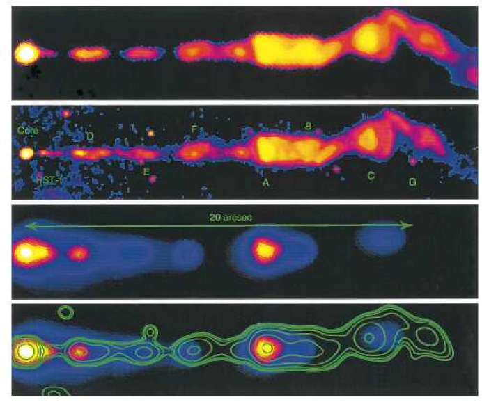
Figure 1: Images of the jet in M87 in three different bands, rotated to be horizontal, and an overlay of optical contours over the X-ray image. Top: Image at 14.435 GHz using the VLA. The spatial resolution is about 0.$"$2. Second panel: The HST Planetary Camera image in the F814W filter. Third panel: Adaptively smoothed Chandra image of the X-ray emission from the jet of M87 in 0.$"$20 pixels. Fourth panel: Smoothed Chandra image overlaid with contours of a Gaussian-smoothed version of the HST image, designed to match the Chandra point response function. The X-ray and optical images have been registered to each other to about 0.$"$05 using the position of the core. The HST and VLA images are displayed using a logarithmic stretch to bring out faint features, while the X-ray image scaling is linear, from [9]

.

The jet in the quasar 3C 273 was observed in radio (MERLIN, 1.647 GHz), in the optics (HST, F622W, centered at 6170A), and in soft X-ray band (0.2-8 keV) by Chandra telescope, with angular resolution $\sim 0".1$. The observations of 3C 273 jet are summarized in [10], and are presented in Fig.2.

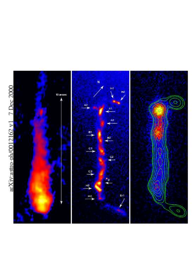
Figure 2: Images of the jet in 3C 273 in three different bands. Left: Image at 1.647 GHz using the MERLIN array. Middle: Hubble Space Telescope Planetary Camera image in the F622W filter (centered at 6170 Å). Right: Raw Chandra image of the X-ray emission from the jet of 3C 273 in $0".1$ bins overlaid with a version of the HST image smoothed with a Gaussian profile in order to match the X-ray imaging resolution. The X-ray and optical images have been registered to each other to about $0".05$ using the position of knot A1. The overall shape of the jet is remarkably similar in length and curvature, but the X-ray emission fades to the end of the jet, so individual C knots are not discernible. The radio emission is much fainter at knot A1 and is displayed with a logarithmic scaling, from [10]

Much longer and fainter jet in radiogalaxy IC 4296 (PKS 1333-33) was observed in radio band (VLA), at bands between 1.3 and 20 cm, with a best resolution $3".2$ . The observations of IC 4296 jet are summarized in [11], and are presented in Fig.3. Total extent of the jet is about 360 kpc Radio observations (MERLIN, 5GHz) of a jet ejection in the microquasar GRS 1915+105, have been presented in [12], see Fig.2 in this paper.

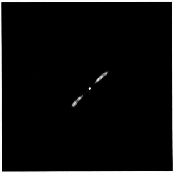
Figure 3: Jet in the radio galaxy IC 4296 at 20 cm with 3”.2 resolution, from [11]

Figure 4: Donald Lynden-Bell and Nikolay Shakura

2 Accretion disk models

2.1 Large scale magnetic accretion

Accretion disk around BH with large scale magnetic field (non-rotating disk) had been investigated in [13, 14]. Self-consistent model of stationary accretion of non-rotating gas, with initially uniform magnetic field, into a black hole (BH) was constructed. At big distances from BH the accretion is almost radial. The magnetic energy, which is small far from BH, in the radial accretion flow is increasing faster than all other types of the energy, and begins to change the flow patterns. Close to the BH the matter flows almost along magnetic field lines, and two flows meat each other in the symmetry plane, perpendicular to the magnetic field direction. Collision of flows leads to development of a turbulence, finite turbulent electrical conductivity, and radial matter flow to BH in the accretion disk, through magnetic field lines. The turbulent electrical conductivity was estimated in [14] as

$$\sigma_{t}=\frac{c^{2}}{\tilde{\alpha}4\pi h\sqrt{P/\rho}},$$ (1)

analogous to the turbulent $\alpha$ - viscosity in the non-magnetized disks, see next section. A magnetic field strength in the vicinity of a stellar BH may reach $10^{7}\,-\,10^{10}$ Gs. At presence of large-scale magnetic field the efficiency of accretion is always large (0.3-0.5) of the rest mass energy flux. Formation of nonrotating disk around BH, supported by magnetic field strength, and self-consistent picture of accretion with account of magnetic field created by induced toroidal electrical currents in the accretion disk are presented in Fig. 5.

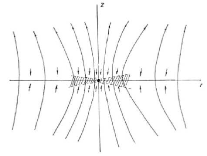
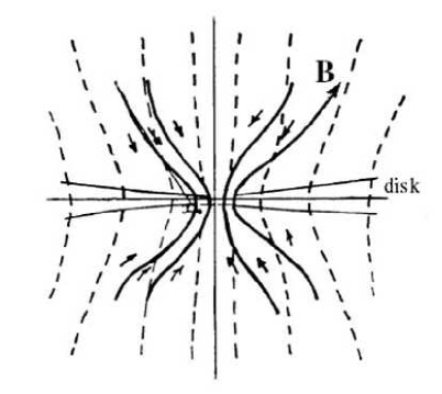
Figure 5: Sketch of the magnetic field threading an accretion disk in a stationary accretion of non-rotating gas. Increase of the field owing to magnetic field freezing, in the accreting matter outside the disk, is shown, from [13] (left). Similar picture, with account of the field generated in the non-rotating accretion disk, from [14], (right).

2.2 Standard accretion disk model

Algebraic relation for construction of the thin accretion disk model were used in [7]. Another presentation, based on so called ”alpha disk” model, suggested in the paper [15], was more attractive, and was used in different types of accretion disks. The small thickness of the disk in comparison with its radius $h\ll r$ indicate to small importance of the pressure gradient $\nabla P$ in comparison with gravity and inertia forces. That leads to a simple radial equilibrium equation denoting the balance between the last two forces occurring when the angular velocity of the disk $\Omega$ is equal to the Keplerian one $\Omega_{K}$,

$$\Omega=\Omega_{K}=\left(\frac{GM}{r^{3}}\right)^{1/2}.$$ (2)

For a thin disk the differential equation for a vertical equilibrium is substituted by an algebraic one, determining the half-thickness of the disk in the form

$$h\approx\frac{1}{\Omega_{K}}\left(2\frac{P}{\rho}\right)^{1/2}.$$ (3)

The balance of angular momentum, related to the $\varphi$ component of the Euler equation has an integral in a stationary case written as

$$\dot{M}(j-j_{in})=-2\pi r^{2}\,2ht_{r\varphi},\quad t_{r\varphi}=\eta r\frac{d\Omega}{dr}.$$ (4)

Here $j=\upsilon_{\varphi}r=\Omega r^{2}$ is the specific angular momentum, $t_{r\varphi}$ is a component of the viscous stress tensor, $\dot{M}>0$ is a mass flux per unit time into a black hole, $j_{in}$ is an integration constant equal to the specific angular momentum of matter falling into a black hole.

$$j_{in}=\Omega_{K}r_{in}^{2},$$ (5)

In the $\alpha$ disk model ($\upsilon_{t}=\alpha\upsilon_{s}$), $\upsilon_{t}$ is an average turbulent velocity, $\upsilon_{s}=\sqrt{P/\rho}$ is a sound speed, the component $t_{r\varphi}$ of the stress tensor is taken [15] proportionally to the isotropic pressure, so that

$$t_{r\varphi}=\rho\upsilon_{t}hr\frac{d\Omega}{dr}\approx\rho\upsilon_{t}\upsilon_{s}=-\alpha\rho\upsilon_{s}^{2}=-\alpha P,\quad\eta=\rho\upsilon_{t}h.$$ (6)

Figure 6: Alexandr Ruzmaikin and Sergey Blinnikov

2.3 Convection and hot corona

Self-consistent structure of the optically thick accretion disk around a black hole has three regions, depending on the origin of pressure and opacity [16], see Fig.7. It was shown in [17], that inner, radiation dominated regions of the accretion disk are convectively unstable, and, therefore, produce a hot corona with electron temperature about $10^{8}\,-\,10^{9}$ K. The model of accretion disk with a hot corona was used for explanation of properties of the X ray source Cygnus X-1, and transition between different states in this source [17].

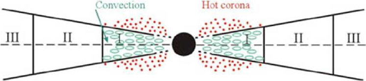
Figure 7: Sketch of picture of a disk accretion on to a black hole at sub-critical luminosity. I - radiation dominated region, electron scattering. II - gas-dominated region, electron scattering. III - gas-dominated region, Krammers opacity; convective region, and hot corona are indicated, from [18].

A presence of a large scale magnetic field in the inner regions of a keplerian accretion disk create mechanism of particle ejection and jet formation [17]. Mechanism for producing fast particles is analogous to the pulsar process. If magnetized matter with low angular momentum falls into the black hole (in addition to the disk accretion), a strong poloidal magnetic field will arise. By analogy to pulsars, rotation will generate an electric field of strength $E\approx−(\upsilon/c)B$ in which electrons are accelerated to energies $\approx R(\upsilon/c)B\,e\approx 3\cdot 10^{4}[B/(10^{7}{\rm Gauss})]$ Mev where $\upsilon/c\approx 0.1$ and $R\approx 10^{7}$ cm is the characteristic scale. In a field $B\approx 10^{7}$ Gauss, such electrons will generate synchrotron radiation with energies up to $\approx 10^{5}$ keV. It would be possible here for $e^{+}e^{−}$ pairs to be formed and to participate in the synchrotron radiation. The flow of high-energy particles along the magnetic field should be visible as a highly collimated flow - jet. Similar model of a jet formation, with account of dynamo processes was considered in the paper [19], see Fig.8.

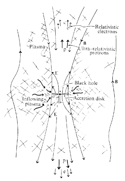
Figure 8: Sketch of the electromagnetic outflows from the two sides of the disk owing to the Faraday unipolar dynamo action of a rotating magnetized disk, from [19].

Figure 9: Igor Novikov and Richard Lovelace

3 Solutions with advection

Standard (local) accretion theory is not correct at luminosity, approaching Eddington limit, and in the vicinity of a last stable orbit around BH. Advection of energy along the accretion disk was taken into account in [20]. In very luminous accretion disks only advective models, qualitatively different from standard ones, give proper results. These models are characterized by decrease of a vertical optical depth with decreasing of a radius, so that accretion disk is optically thick at larger, and optically thin at smaller radiuses, with a gradual transition between these regions [21, 22]. Set of equations for ”$\alpha$ P” viscosity prescription

$$t_{r\varphi}=\alpha P,$$ (7)

where $\alpha$ is a parameter, $\alpha\leq 1$, with advection, had been solved in [21]. Radiative cooling term $Q^{-}$, and equation of state, describing smooth optically thick-thin transition were take from [23] as

$$Q^{-}={2aT^{4}c\over 3\tau_{0}}\left(1+\frac{4}{3\tau_{0}}+\frac{2}{3\tau_{*}^{2}}\right)^{-1},$$ (8)

$$P=\rho{\cal R}T\,+\,{aT^{4}\over 3}\left(1+\frac{4}{3\tau_{0}}\right)\left(1+\frac{4}{3\tau_{0}}\textsl{+}\frac{2}{3\tau_{*}^{2}}\right)^{-1}.$$ (9)

Here $\tau_{0}=\kappa\rho h$ is a total Thomson scattering depth of the disk and

$$\tau_{*}=\left(\tau_{0}\tau_{\alpha}\right)^{1/2}$$ (10)

is the effective optical depth valid for the case $\tau_{0}\gg\tau_{\alpha}$, which takes place in a region with intermediate optical depths, $\tau_{\alpha}$ is the optical depth with respect to bremsstrahlung absorption,

$$\tau_{\alpha}\simeq 5.2\cdot 10^{21}{\rho^{2}T^{1/2}h\over acT^{4}}~{}.$$ (11)

A numerical solution of the set of the following non-dimensional equations was obtained in [21]. Gravitational potential $\varphi_{g}$ of Paczynski-Witta [24] was used, accounting for some effects of general relativity:

$$\varphi_{g}=\frac{GM}{r-2r_{g}},$$ (12)

$$r{\upsilon^{\prime}\over\upsilon}={N\over D}~{},$$ (13)

$$r{c_{s}^{\prime}\over c_{s}}=1+\frac{c^{2}\,x^{2}}{{c}_{s}^{2}}\left(\tilde{\Omega}^{2}-\frac{1}{x(x-2)^{2}}\right)+\frac{3x-2}{2(x-2)}-\left(\frac{{\upsilon}^{2}}{{c}_{s}^{2}}-1\right){N\over D}~{}~{},$$ (14)

where the notations $N$ and $D$ denote algebraical expressions, depending only on $r$, $\upsilon$, $c_{s}$, and $\ell_{\rm in}$.

$$\Omega={\ell_{in}\over r^{2}}+\alpha{c_{s}^{2}\over\upsilon r}~{}.$$ (15)

$$(1-\beta)P={aT^{4}\over 3}\left(1+\frac{4}{3\tau_{0}}\right)\left(1+\frac{4}{3\tau_{0}}\textsl{+}\frac{2}{3\tau_{*}^{2}}\right)^{-1}.$$ (16)

$$x=\frac{r}{r_{g}},\quad r_{g}=\frac{GM}{c^{2}},\quad\widetilde{\Omega}=\frac{\Omega r_{g}}{c},\quad\beta=\frac{P_{g}}{P}=\frac{{\cal R}T}{c_{s}^{2}},\quad c_{s}^{2}=\frac{P}{\rho},\quad T=\beta\frac{c_{s}^{2}}{\cal R}$$ (17)

Here $\ell_{in}$ is a specific angular momentum on the last stable orbit. Solution of equations (12)-(14), with account of (15)-(17), for $\tau_{0}(r_{*})$, $\tau_{*}(r_{*})$, $T(r_{*})$ are given in Figs.10,11, from [25].

Figure 10: The dependence of the Thompson scattering depth (left), and the effective optical depth (right) on the radius , and for the models with $\alpha=0.5$ and $M_{BH}=10M_{\odot}$. Dashed lines correspond to the solutions without advection and $\dot{m}<\dot{m}_{cr}=36$. Dotted lines correspond to the non-physical solutions without advection for $\dot{m}=\dot{m}_{cr}=36$ and $\dot{m}=50$ (from the center to the edge of the picture respectively). Solid lines correspond to the solutions with advection and the mass accretion rate higher than the critical one. Thick solid line corresponds to $\dot{m}=36.0$, and the thin solid line to $\dot{m}=50.0$, $\dot{m}=\dot{M}/\dot{M}_{\rm Edd}$, where $\dot{M}_{\rm Edd}=L_{\rm Edd}/c^{2},\,\,\,L_{\rm Edd}=4\pi cGMm_{p}/\sigma_{T}$; $r_{*}\equiv x$, from [25].

Figure 11: The dependence of the temperature on the radius for the same models as in Fig.10; $r_{*}\equiv x$, from [25].

In a rotating BH, with the Kerr metric, the temperature in the optically thin region exceeds 500 keV, when an intensive $e^{+}e^{-}$ pair creation takes place [26].

Figure 12: Julia Artemova and Alexandr Klepnev

4 Magnetic jet collimation

Observations of extragalactic jets in different objects distinctly show existence of bright knots along a whole jet in different wavelengths, Fig.13, see also Figs.1,2.

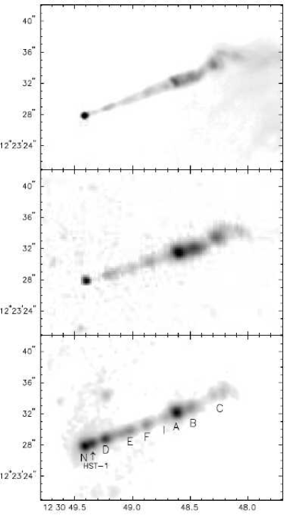
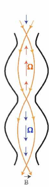
Figure 13: Gray-scale representations of a 6 cm radio (top; resolution 0$"$4); an optical V band (middle, resolution 0$"$7); and the Chandra X-ray (bottom, resolution 0$"$7; 0.1 - 10 keV band) image. The labels in the lower panel refer to the knots vertically above the label. N is the nucleus, from [27] (left). Scheme of magnetic collimation due to torsional oscillations, from [4] (right).

It was shown by optical photoelectric polarization observations of the jet in M87 [28], that polarization angles in neighboring blobs are orthogonally related, see Fig.14.

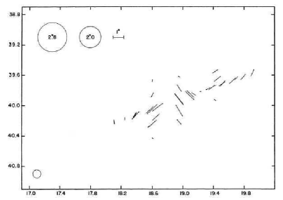
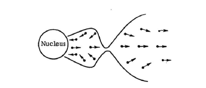
Figure 14: Photoelectric polarization observations of the jet in M87. The polarization angles in neighboring blobs are orthogonally related. The relative sizes of the diaphragms used are shown in the upper left of the figure. The position of the nucleus of M87 is shown by a small open circle in the lower left, from [28] (left). Magnetically collimated jet by inductance-capacitance oscillations in the blob, from [29] (right).

This behavior was interpreted in the model of magnetic collimation [29], where initial charge separation in the neighboring blobs leads to oscillating electrical current, as in a capacitance-inductance system. This current produces azimuthal magnetic field, preventing jet expansion and disappearance. The period of oscillations should be $P_{osc}\sim D/c$, where $D$ is a size of the blob in the jet, see Fig.14.

Magnetic collimation, connected with torsional oscillations of a cylinder with elongated magnetic field, was considered in [4]. Instead of initial blobs with charge separation, there is a cylinder with a periodically distributed initial rotation around the cylinder axis. The stabilizing azimuthal magnetic field is created here by torsional oscillations, where charge separation is not necessary. Approximate simplified model is developed. Ordinary differential equation is derived, and solved numerically, what gives a possibility to estimate quantitatively the range of parameters where jets may be stabilized by torsional oscillations. The polytropic equation of state $P=K\,\rho^{\gamma}$, with $\gamma=1$, was considered. Using approximate relations

$$\upsilon_{r}=r\,a(t,z),\quad\upsilon_{\varphi}=r\,\Omega(t,z),\quad\upsilon_{z}=0,$$ (18)

introduce non-dimensional variables in the plane, where angular velocity $\Omega$ remains zero during oscillations. the variables in this plane are denoted by ”tilde”.

$$\tau=\omega t,\,\,y=\frac{\tilde{R}}{R_{0}},\,\,z=\frac{a\tilde{R}}{a_{0}R_{0}},\,\,a_{0}=\frac{K}{\omega R_{0}^{2}}=\omega,\,\,R_{0}=\frac{\sqrt{K}}{\omega},$$ (19)

Here $\omega$ is the frequency of radial oscillations. In these variables differential equations have a form

$$\frac{dy}{d\tau}=z,\quad\frac{dz}{d\tau}=\frac{1}{y}(1-D\sin^{2}\tau);\,\,\,\,y=1,\,\,z=0\,\,{\rm at}\,\,\tau=0.$$ (20)

Therefore, the problem is reduced to a system (20) with only one non-dimensional parameter

$$D=\frac{1}{2\pi KC_{m}}\left(\frac{C_{b}\Omega_{0}}{z_{0}\omega}\right)^{2},$$

where $C_{b}$ and $C_{m}$ are integrals of motion, see [4] for details. Solution of this nonlinear system changes qualitatively with changing of the parameter $D$. The solution of this system was obtained numerically for $D$ between 1.5, and 3.1. Roughly the solutions may be divided into 3 groups.

1. At $D$ ¡ 2.1 there is no confinement, and radius grows to infinity after several low-amplitude oscillations.

2. With growing of $D$, the amplitude of torsional oscillations $\Omega_{0}$ increases, and at $D=2.1$ radius is not growing to infinity, but is oscillating around some average value, forming rather complicated curve (Fig.15, left).

3. At $D$= 2.28 and larger the radius finally goes to zero with time, forming separate blobs, but with different behavior, depending on $D$. At $D$ between 2.28 and 2.9 the dependence of the radius $y$ with time may be very complicated, consisting of low-amplitude and large-amplitude oscillations, which finally lead to zero. The time at which radius becomes zero depends on $D$ in rather peculiar way, and may happen at $\tau\leq 100$, like at $D$=2.4, 2.6; or goes trough very large radius, and returned back to zero value at very large time $\tau\sim 10^{7}$ at $D$=2.5. From $D=3$ and larger the radius goes to zero at $\tau<2.5$ (Fig.15, right). before the right side of the second equation (20) returned to the positive value. The results of numerical solution are represented in Figs. 1-18 of [4]. Frequency of oscillations $\omega$ is taken from linear approximation. When y(0) is different from 1, there is a larger variety of solutions: regular and chaotic. Development of chaos of these oscillations is analysed in [30]

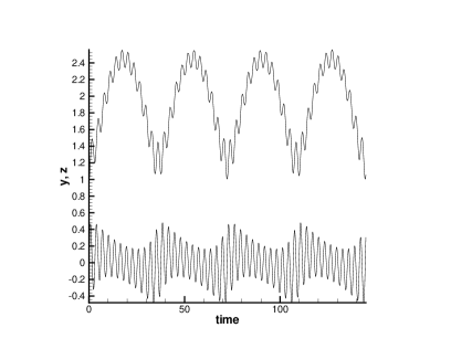
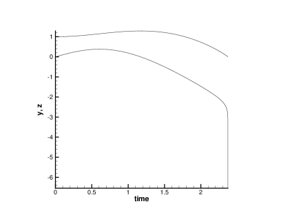
Figure 15: Time dependence of non-dimensional radius $y$ (upper curve), and non-dimensional velocity $z$ (lower curve), for $D=2.1$ (left), and $D=3.1$ (right).

On the edge of the cylinder the rotational velocity cannot exceed the light velocity, so the solution with initial conditions, corresponding to $y_{0}=1$, has a physical sense only at $\upsilon_{s}^{2}<\frac{c^{2}}{2\pi^{2}D\alpha_{n}^{2}}\approx\frac{c^{2}}{40\alpha_{n}^{2}}$, where $\omega=\alpha_{n}\,k\,V_{A},\,\,\alpha_{n}<1,\,\,k=\frac{2\pi}{z_{0}}$, $z_{0}$ is the space period of the torsional oscillations along $z$ axis, $V_{A}$ is Alfven velocity. Taking $\alpha_{n}^{2}=0.1$ for a strongly non-linear oscillations we obtain a very moderate restriction $\upsilon_{s0}^{2}<\frac{c^{2}}{4}$. While in the intermediate collimation regime the outer tangential velocity is not changing significantly, this restriction would be enough also for the whole period of the time. To have the sound velocity not exceeding $c/2$, the jet should contain baryons, which density $\rho_{0}$ cannot be very small, and its input in the total density in the jet should be larger than about 30% [4].

5 Laboratory experiments and numerical simulations

Experiments aimed at studying the spatial distributions of beams of accelerated protons using CR-39 track detectors were carried out at the Neodim 10- TW picosecond laser facility [31], see Fig.16

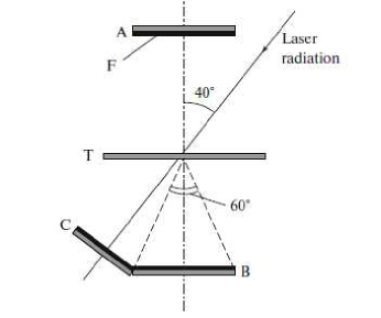
Figure 16: Scheme for the experiments investigating the spatial distribution of beams of accelerated protons. A, B, C are the CR-39 track detectors, F are filters of Al with thicknesses of 11 - 80 $\mu$m, and T is the target of Cu (30 and 50 $\mu$m) or Ta (50 $\mu$m); from [32].

Numerical simulations of the flow of the matter from the target, heated by the laser beam, have been presented in [32]. Similarity conditions permit to compare parameters of laboratory experiments with jets on the from AGN’s and quasars, see Tabl.

Laboratory jet	Jets from AGN nuclei (VLBI)
after scaling, from [32]
$x=(0.3\div 3)\times 10^{18}$ cm	3$\times 10^{18}$ cm,
$t=(0.3\div 3)\times 10^{9}$ s	$10^{8}$ s,
$\upsilon=10^{9}$ cm/s	$3\times 10^{10}$ cm/s,
$\rho=10^{-26}$ g/cm3	$10^{-26}$ g/cm3,
$n=10^{-2}$ cm-3	$10^{-2}$ cm-3,
$H=10^{-1}$ Gs	$10^{-3}$ Gs,
$T=10^{11}$ K	$10^{11}$ K.

Analysis of the experiment showed the formation of a jet due to heating of the foil, with the geometry of the incident laser beam not being important. This means that the mathematical model for the formation of the jet can be constructed in an axially symmetric approximation, assuming that the laser-heated spot is circular. MHD equations were solved in 2-D problem with a finite electrical conductivity, without gravity. The scheme of the experiment and the region of modeling are presented in Figs.17. The detailed description of the method and numerical results are presented in [32].

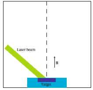
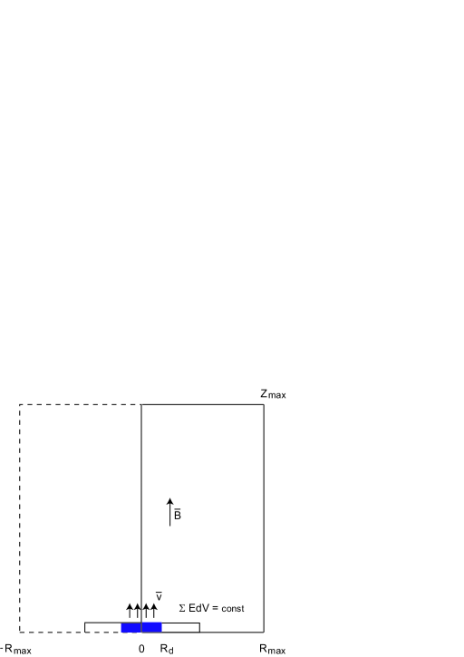
Figure 17: Experiment scheme (left). Region of modeling (right), from [32].

The example of results of numerical calculations, performed by O.D. Toropina, is presented in Fig.18 from [32], where detailed results of calculations are given. The ring structure, observed on the photo of the experiment, is visible on this figure. The computations are performed for the target density $\rho\approx 300\rho_{0}$, where $\rho_{0}$ is a background density. The important non-dimensional parameter $\beta$ is a ratio of the initial gas pressure at the jet origin to the initial magnetic pressere

$$\beta=\frac{8\pi P_{0jet}}{H_{0}^{2}}=\frac{2}{\gamma}\frac{c_{s0}^{2}}{V_{A0}^{2}}\;.$$ (21)

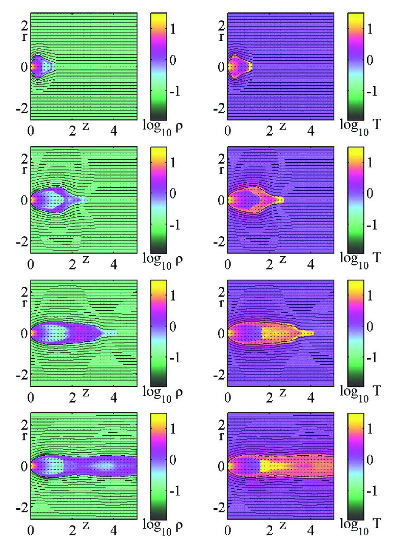
Figure 18: Time dependence of the flow, induced by the laser beam, in presence of the poloidal magnetic field with $\beta=0.1$ at time moments t = 5, t = 10, t = 25, t = 45. Density is given in the left column, temperature is to the right, from [32].

6 Conclusion - Problems

1. Jet origin (blobs or continuous injection; radiation pressure or explosions) BLOBS -!?

2. Jet collimation (magnetic, or outer pressure, or kinematic)

3. Jet constitution (baryonic or pure leptonic) Baryonic -!?

4. Particle acceleration (shocks, reconnection, kinetic)

5. Radiation mechanisms (synchrotron, inverse Compton, nuclear processes)

Jets in Lab should help to answer!

- [1] G.S. Bisnovatyi-Kogan, R.V.L. Lovelace, Astron. Ap., 296, L17 (1995)
- [2] G.S. Bisnovatyi-Kogan, B.V. Komberg, A.M. Friedman, Sov. Astronomy, 13, 369 (1969)
- [3] Blandford R.D., Rees M.J., MNRAS, 169, 395 (1974)
- [4] Bisnovatyi-Kogan G.S., MNRAS 376, 457 (2007)
- [5] Krauz V.I. et al., Physics of Plasma 36, 997 ( 2010)
- [6] Belyaev V.S., Quantum Electronics, 34, 41 ( 2004)
- [7] Lynden-Bell D. Nature, 223, 690 (1969)
- [8] Mirabel I.F., Rodriguez L.F., Cordier B., Paul J., Lebrun F. Nature 358, 215 (1992)
- [9] Marshall H.L., Miller B.P., Davis D.S., et al. ApJ, 564, 683 (2002)
- [10] Marshall H.L., Harris D.E., Grimes J.P., et al. ApJL, 549, L167 (2001)
- [11] Killeen, N. E. B.; Bicknell, G. V.; Ekers, R. D. ApJ, 302, 306 (1986)
- [12] Fender R.P., Garrington S.T., McKay D.J., et al., MNRAS 304, 865 (1999)
- [13] Bisnovatyi-Kogan G.S., & Ruzmaikin A.A., Astrophys. and Space Sci. 28, 45 (1974)
- [14] Bisnovatyi-Kogan G.S., & Ruzmaikin A.A., Astrophys. and Space Sci., 42, 401 (1976)
- [15] Shakura N.I., Sov. Astron., 16, 756 (1973)
- [16] Shakura N.I. & Sunyaev R.A., A&A, 24, 337 ( 1973)
- [17] Bisnovatyi-Kogan G.S., and Blinnikov S.I., Sov.Astron.Lett. 2, 191 (1976)
- [18] Bisnovatyi-Kogan G.S. Biulleten’ Abastuman. Astrofiz. Observ., no. 58, pp. 175-210 (1985). In Russian.
- [19] Lovelace, R.V.E. Nature 262, 649 (1976)
- [20] Paczyński B., Bisnovatyi-Kogan G., Acta Astronomica 31, 283, (1981)
- [21] Artemova Yu.V., Bisnovatyi-Kogan G.S., Igumenshchev I.V., Novikov I.D., ApJ 637, 968 (2006)
- [22] Klepnev A.S., and Bisnovatyi-Kogan G.S., Astrophysics 53, 409 (2010)
- [23] Artemova I.V., Bisnovatyi-Kogan G.S., Bjoernsson G., Novikov I.D., ApJ 456, 119 (1996)
- [24] Paczyński B., Wiita P.J., Astronomy and Astrophysics 88, 23 (1980)
- [25] Artemova Yu.V., Bisnovatyi-Kogan G.S., Igumenshchev I.V., Novikov I.D., in ”Astrophysics and Cosmology After Gamow”. Eds. G. S. Bisnovaty-Kogan, S. Silich, E. Terlevich, R. Terlevich and A. Zhuk. Cambridge Scientific Publishers, Cambridge, UK, 2007, p.311 (2007)
- [26] Bisnovatyi-Kogan G.S. Stellar Physics 2: Stellar Evolution and Stability. Springer-Verlag Berlin Heidelberg, p.291 (2011)
- [27] Wilson A.S., Yang Y., ApJ 568, 133 (2002)
- [28] Hiltner W.A., ApJL 130, 340 (1959)
- [29] Bisnovatyi-Kogan G.S., Komberg B.V., Fridman A.M., Soviet Astronomy, 13, 369 (1969),
- [30] Bisnovatyi-Kogan G.S., Neishtadt A.I., Seidov Z.F., Tsupko O.Yu., Krivosheev Yu.M., MNRAS 416, 747 (2011)
- [31] Belyaev V.S. , Vinogradov V.I. , Matafonov A.P. et al., Laser Phys. 16, 477 (2006)
- [32] Belyaev V.S., Toropina O.D., Bisnovatyi-Kogan G.S., Moiseenko S.G., et al. Astronomy Reports, 62, 162 (2018)