The relativistic jet of the $\gamma$-ray emitting narrow-line Seyfert 1 galaxy PKS J1222$+$0413

Abstract

We present a multi-frequency study of PKS J1222$+$0413 (4C $+04.42$), currently the highest redshift $\gamma$-ray emitting narrow-line Seyfert 1 ($\gamma$-NLS1). We assemble a broad spectral energy distribution (SED) including previously unpublished datasets: X-ray data obtained with the NuSTAR and Neil Gehrels Swift observatories; near-infrared, optical and UV spectroscopy obtained with VLT X-shooter; and multiband radio data from the Effelsberg telescope. These new observations are supplemented by archival data from the literature. We apply physical models to the broadband SED, parameterising the accretion flow and jet emission to investigate the disc-jet connection. PKS J1222$+$0413 has a much greater black hole mass than most other NLS1s, $M_{\mathrm{BH}}\approx{\color[rgb]{0,0,0}2}\times 10^{8}$ M_☉, similar to those found in flat spectrum radio quasars (FSRQs). Therefore this source provides insight into how the jets of $\gamma$-NLS1s relate to those of FSRQs.

1 Introduction

The relativistic jets present in a subset of active galactic nuclei (AGN) are among the most energetic phenomena in the Universe. Matter transported in these jets is expelled from the nucleus at velocities approaching the speed of light. These jets are highly-collimated and can extend for great distances beyond the galaxy in which they originate, far out into intergalactic space. The most spectacular examples of these are the jets of blazars, in which the jet is aligned to our line of sight. As a result of relativistic beaming, the emission from the jet is amplified and non-thermal emission from the jet can be detected across the whole electromagnetic spectrum from radio to $\gamma$-rays.

Blazar jet emission is understood to originate from highly energetic electrons within the jet. Synchrotron emission resulting from the electrons entrained in magnetic field lines in the jet produces a low-frequency peak (at radio-to-X-ray frequencies) in the spectral energy distribution (SED). A second, higher-frequency, peak (at X-ray-to-$\gamma$-ray frequencies) results from the up-scattering of soft seed photons; the peak frequency and luminosity of this feature depends on the environment in which the electrons cool. Flat spectrum radio quasars (FSRQs) are high accretion-rate systems ($L/L_{\mathrm{Edd}}\sim 0.1$) with a luminous accretion disc and broad line region (BLR). In FSRQs, electrons within the jet cool by up-scattering seed photons originating in the accretion flow (from the disc and its corona, the BLR and extended, dusty torus) via the external Compton (EC) mechanism (e.g. Gardner & Done 2018). In contrast, the dearth of external seed photons in low accretion rate BL Lacertae objects (BL Lacs) means the electrons cool by Compton upscattering the synchrotron photons they emit, via the synchrotron self-Compton (SSC) process (e.g. Gardner & Done 2014, Ghisellini & Tavecchio 2009). BL Lacs and FSRQs form a ‘blazar sequence’ (Fossati et al. 1998, Ghisellini et al. 2017) from the low-power, high-frequency peaked SEDs of BL Lacs to high-power, low-frequency peaked SEDs of FSRQs.

Ghisellini et al. (2014) found that the jet power of FSRQs and BL Lacs is correlated with, and often exceeds, the accretion power. It has been proposed that jets are able to draw power from the angular momentum of spinning black holes (BHs) (Blandford & Znajek 1977) or may be launched by a high concentration of accumulated magnetic flux (Sikora & Begelman 2013), although the launching and powering mechanisms of jets are still debated. Some early studies thought that the mass of the BH must play a role, since FSRQs and BL Lacs all have high-mass BHs ($\log(M_{\mathrm{BH}}/\mathrm{M}_{\sun})\gtrsim 8$–9, Ghisellini et al. 2010) and are hosted in large, elliptical galaxies. This view changed with the Fermi Gamma-Ray Space Telescope detection of $\gamma$-ray emission from narrow-line Seyfert 1 galaxies (Abdo et al. 2009). NLS1s usually have low BH masses $\langle\log(M_{\mathrm{BH}}/\mathrm{M}_{\sun})\rangle=6.9$, high accretion rates (Rakshit et al. 2017) and are typically found in spiral galaxies. With luminous accretion discs and BLRs, the electron cooling environment of their jets (and hence the spectral properties of their non-thermal SEDs) are very similar to those of FSRQs, but at much lower jet powers. However, where (and whether) $\gamma$-NLS1s fit on the standard blazar sequence is still an open question. By investigating the jet and accretion flow properties of $\gamma$-NLS1s we can better understand how relativistic jets scale with the mass and accretion rate of the central BH.

1.1 The source PKS J1222$+$0413

PKS J1222$+$0413 (RA: 12 22 22.548, Dec: $+$04 13 15.75) was identified as a $\gamma$-ray NLS1 candidate by Yao et al. (2015) and, at redshift $z=0.9662$, is currently the most distant example of this class known. From its SDSS spectrum, they determined its mass to be $M_{\mathrm{BH}}=1.8$–$2.0\times 10^{8}$ M_☉. Its simultaneous and quasi-simultaneous SED was studied by Giommi et al. (2012), although at the time it was not known to be a NLS1. Like 1H 0323$+$342, which was studied in great detail by Kynoch et al. (2018), the accretion disc of PKS J1222$+$0413 is a prominent feature in its spectral energy distribution, unlike other $\gamma$-NLS1s which are more jet-dominated. PKS J1222$+$0413 is therefore another ideal object in which to examine the disc-jet connection. We present new data from NuSTAR, VLT X-shooter and Effelsberg. The VLT X-shooter data allows us to investigate the NLS1 nature of the source and measure the AGN continuum emission from the accretion disc. The 0.3–10 keV X-ray band has been shown to contain contributions from both the accretion flow and jet (e.g. Kynoch et al. 2018, Larsson et al. 2018) whereas the higher-energy X-rays, sampled by NuSTAR and Swift BAT, are jet-dominated.

Throughout this paper, we assume a $\Lambda$CDM cosmology with $H_{0}=70$ km s^-1 Mpc^-1, $\Omega_{\mathrm{m}}=0.3$ and $\Omega_{\Lambda}=0.7$. Therefore the redshift $z=0.9662$ implies a luminosity distance of 6332.3 Mpc and a flux-to-luminosity conversion factor of $4.80\times 10^{57}$ cm². Length scales are often quoted in gravitational radii, $R_{\mathrm{g}}=GM_{\mathrm{BH}}/c^{2}={\color[rgb]{0,0,0}2.95}\times 10^{11}$ m $={\color[rgb]{0,0,0}1.14}\times 10^{-2}$ light days for our derived mass.

2 X-Shooter spectroscopy

2.1 The observations and data reduction

We have conducted X-shooter (Vernet et al. 2011) observations of five $\gamma$-NLS1s (including PKS J1222$+$0413) in the Southern and equatorial sky, with the aim of characterising their accretion disc continuum and emission line properties. Our near-infrared, optical and ultraviolet spectra were obtained using X-shooter which is a wide-band, intermediate resolution spectrograph developed for the Very Large Telescope (VLT). The instrument is mounted on the VLT’s 8.2 m Unit Telescope 2 at ESO Paranal in Chile. Dichroics in the instrument reflect light into ultraviolet-blue (UVB) and visible light (VIS) arms and transmit the remaining light to the near-infrared (NIR) arm. At the end of each arm is an échelle spectrograph, with the UVB spectrograph covering the 300–550 nm range, the VIS spectrograph covering 550-1010 nm and the NIR spectrograph covering 1000–2500 nm. Thus, by operating these three spectrographs simultaneously, X-shooter offers a very wide wavelength coverage from 300 to 2500 nm. We used the $0.9^{\prime\prime}\times 11^{\prime\prime}$, $1.2^{\prime\prime}\times 11^{\prime\prime}$, $1.3^{\prime\prime}\times 11^{\prime\prime}$ slits, giving spectral resolutions $R\approx 5600$, 6700 and 4000 in the IR, optical and UV spectra, respectively. The observation was conducted on 3 April 2017 under favourable weather conditions with clear skies and seeing $\approx 1^{\prime\prime}$ at 500 nm. The on-source integration time was 1 hour and the mean S/N achieved in the IR, optical and UV spectra were 12, 16 and 23, respectively.

The data reduction was performed with the ESO reflex software which outputs wavelength- and flux-calibrated 1D spectra. Corrections for telluric absorption in the optical and UV spectra were performed with the xtellcor_general tool available as part of the spextool IDL package (Vacca et al. 2003; Cushing et al. 2004).

To sample the AGN continuum emission within the X-shooter spectral range, we averaged the flux in several emission line free windows of width 50 Å. These were (rest frame): 1660, 2000 and 2200 Å observed in the UV; 3050, 3930 and 4205 Å observed in the optical; 5100, 6205, 8600 and 11020 Å observed in the IR. Five of these windows are those suggested by Capellupo et al. (2015) for the purpose of modelling accretion disc emission in SEDs.

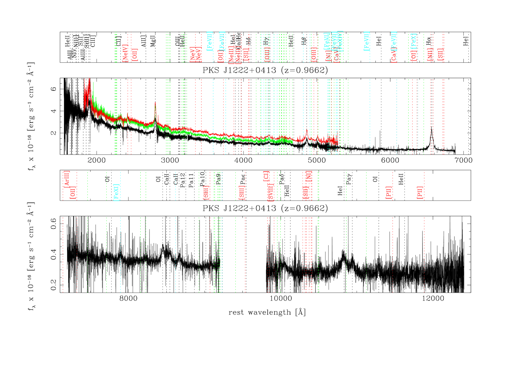
Figure 1: VLT X-shooter spectra (black) taken 3 April 2017. SDSS spectra taken 13 February 2008 and 26 March 2011 are overplotted in green and red, respectively.

2.2 Estimates of the black hole mass

We estimate the BH mass of PKS J1222$+$0413 using virial scaling relations employing the full widths at half-maximum (FWHMs) of the broad components of permitted emission lines (namely H$\upalpha$, H$\upbeta$ and Mg ii) and the ionising continuum luminosities measured at 5100 and 3000 Å in the rest frame. All of these quantities are covered simultaneously by our X-shooter spectrum. The measurements of the 5100 Å and 3000 Å continuum luminosities are straightforward and we get values of $\log\nu L_{\rm 5100\AA}=45.56$ erg s^-1 and $\log\nu L_{\rm 3000\AA}=45.66$ erg s^-1, respectively.

Before measuring the emission line widths and fluxes we first modelled and subtracted Fe ii emission complexes around H$\upbeta$ and Mg ii following the method described in Landt et al. (2017). The Mg ii$\lambda 2008$ emission line is a blended doublet of lines centred at 2795 and 2802 Å with an intensity ratio of approximately 1.2:1. To determine the widths of the individual broad lines we model the doublet as the sum of two broad Lorentzians with their intensities and wavelength separation fixed to the theoretical values. Additionally, we include two narrow Gaussian lines to account for any contribution from the narrow emission line region. The narrow lines are fixed to the same intensity ratio and separation, and their widths are limited to be in the range $300\leqslant\mathrm{FWHM}\leqslant 900$ km s^-1. The fitting is performed with a custom python script employing the lmfit package, which uses the Levenberg-Marquardt method of least-squares fitting. We find that the inclusion of the narrow lines does not improve the fit therefore we model the doublet simply as the sum of two Lorentzians (see Figure 2). The FWHM of these lines is $\approx 1750$ km s^-1. Using the recently-recalibrated BH mass relationship of Mejía-Restrepo et al. (2016), we estimate the BH mass to be $\left({\color[rgb]{0,0,0}2.6^{+2.0}_{-1.2}}\right)\times 10^{8}$ M_☉.

In order to correctly measure the widths of the Balmer emission line broad components, we need to subtract any contribution from the narrow line region. Commonly, the [O iii]$\lambda 5007$ forbidden emission line is taken as being representative of the narrow emission line profiles. A narrow line with the same profile as [O iii]$\lambda 5007$ is then subtracted from the (total) permitted line profiles, in principle leaving only their broad components. However, the [O iii]$\lambda 5007$ line is very weak so its profile is unsuitable for this purpose. Instead, we measure its total flux and use this to estimate the likely scaled flux of narrow H$\upbeta$ in the following way. ‘Normal’ Seyferts have a typical [O iii]$\lambda 5007$ to narrow H$\upbeta$ flux ratio of $\approx 10$ (e.g. Cohen 1983) and analyses of large samples have found consistent narrow line ratios in NLS1s (e.g. Véron-Cetty et al. 2001; Zhou et al. 2006; Rakshit et al. 2017). We estimate the [O iii]$\lambda 5007$ line luminosity by integrating the observed flux density and we determine $\log L_{\mathrm{[O\textsc{iii}]}}=42.3$ erg s^-1. Assuming the ratio $L_{\mathrm{[O\textsc{iii}]}}/L^{\mathrm{n}}_{\mathrm{H}\upbeta}=10$ for our source, $\log L^{\mathrm{n}}_{\mathrm{H\upbeta}}=41.3$ erg s^-1, which is negligible compared to the total line luminosity $\log L_{\rm H\upbeta}=43.11$ erg s^-1. Clearly, if the contribution from the narrow line component is negligible then we can measure the FWHM of H$\upbeta$ directly from its observed profile and we obtain $\mathrm{FWHM(H\upbeta)}\approx 1760$ km s^-1, which is extremely close to the FWHMs of the blended components of the Mg ii doublet. Using the Bentz et al. (2013) radius-luminosity relationship for the H$\upbeta$ line, derived from optical reverberation mapping results, we determine a BLR radius of $260^{+91}_{-67}$ light-days. Then, assuming a geometrical scaling factor of $f=1.4$ appropriate for FWHM measures (Onken et al., 2004), we derive a BH mass of $\left({\color[rgb]{0,0,0}2.2^{+0.8}_{-0.5}}\right)\times 10^{8}$ M_☉. We measure a $\mathrm{FWHM}={\color[rgb]{0,0,0}1850}$ km s^-1 for H$\upalpha$. Using the BH mass relationship of Mejía-Restrepo et al. (2016) we estimate the BH mass to be $\left({\color[rgb]{0,0,0}2.5^{+1.1}_{-0.8}}\right)\times 10^{8}$ M_☉. These mass estimates and the relations used to calculate them are tabulated in Table 1.

Table 1: Estimates of the black hole mass

Measurements	$M_{\rm BH}$	Reference
	(108 M☉)
$\log\nu L_{\rm 3000\AA}=45.66$ erg s-1	2.6${}^{+2.0}_{-1.2}$	Table 7 of Mejía-Restrepo et al. (2016)
FWHM(Mg ii)=1750 km s-1
$\log\nu L_{\rm 5100\AA}=45.56$ erg s-1	2.5${}^{+1.1}_{-0.8}$	Table 7 of Mejía-Restrepo et al. (2016)
FWHM(H$\upalpha$)=1850 km s-1
$\log\nu L_{\rm 5100\AA}=45.56$ erg s-1	2.2${}^{+0.8}_{-0.5}$	Table 14 of Bentz et al. (2013)
FWHM(H$\upbeta$)=1760 km s-1
$\log L_{\rm H\upalpha}={\color[rgb]{0,0,0}43.65}$ erg s-1	0.5${}^{+0.3}_{-0.2}$	Table 7 of Mejía-Restrepo et al. (2016)
FWHM(H$\upalpha$)=1850 km s-1
$\log L_{\rm H\upbeta}={\color[rgb]{0,0,0}43.11}$ erg s-1	0.8${}^{+0.5}_{-0.3}$	Table 2 of Greene et al. (2010)
FWHM(H$\upbeta$)=1760 km s-1

The $1\sigma$ error is derived from the instrinsic scatter rather than the errors on the best-fit parameter values.

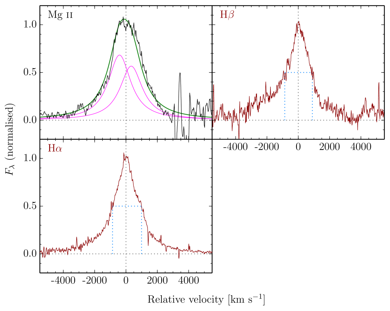
Figure 2: The profiles of the three broad emission lines H$\upalpha$, H$\upbeta$ and Mg ii that we used to estimate the BH mass for PKS J1222$+$0413. The profiles are shown in velocity space relative to the expected rest-frame wavelength and have been Fe ii- and continuum-subtracted and normalized to the same peak intensity. In the top left panel, the Mg ii profile has been modelled as the sum of two Lorentzians (magenta) and the total modelled profile is shown in green. Since the narrow line region likely makes a negligible contribution to the Balmer line fluxes, the FWHM of the broad H$\upbeta$ and H$\upalpha$ lines may be estimated directly from the observed line profiles, as shown.

Our estimates of the BH mass based on the ionising continuum luminosity and the width of the broad Balmer emission lines H$\upalpha$ and H$\upbeta$ and the Mg ii emission line give a very small range of values of $\approx{\color[rgb]{0,0,0}2.2-2.6}\times 10^{8}$ M_☉, with an average value of $\approx{\color[rgb]{0,0,0}2.4}\times 10^{8}$ M_☉. This excellent agreement between the three estimates is remarkable, given that the relationships upon which they are based have uncertainties of the order of $\sim 30-80\%$ at the $1\sigma$ level.

Alternative methods to estimate the BH mass, which are based on the line luminosity instead of the ionising continuum luminosity (e.g. Greene et al. 2010; Mejía-Restrepo et al. 2016) are also considered and we quote the results in Table 1. These estimates are in the range of $\sim{\color[rgb]{0,0,0}0.5-0.8}\times 10^{8}$ M_☉, which are a factor of $\sim 4$ smaller than found previously. Since we use the same broad line FWHMs in both estimates, the difference in the estimated masses is due to the different choice of proxy for the ionising luminosity (i.e. the monochromatic continuum luminosity or the broad line luminosity). We argue that it is unlikely that the difference in masses is due to an overestimation of the 3000 Å and 5100 Å luminosities because of unsubtracted emission from the host galaxy or the jet. Firstly, for a bright AGN such as this, we expect the host galaxy emission to be relatively weak, as was previously noted by Yao et al. (2015). Certainly at 3000 Å in the rest frame the host galaxy emission will be negligible. Second, estimates of the mass depend approximately on the square root of the (continuum or line) luminosity. The two mass estimation methods would agree only if we have over-estimated the AGN contribution to $L_{\mathrm{5100$\mathrm{\SIUnitSymbolAngstrom}$}}$ and $L_{\mathrm{3000$\mathrm{\SIUnitSymbolAngstrom}$}}$ by a factor $\sim 4^{2}$, which is highly unlikely. If we were to believe that $L_{\mathrm{5100$\mathrm{\SIUnitSymbolAngstrom}$}}$ and $L_{\mathrm{3000$\mathrm{\SIUnitSymbolAngstrom}$}}$ are contaminated then since the mass estimates using both luminosities are similarly high, they must contain an approximately equal fraction of contaminating emission (i.e. the contaminating non-acrretion disc emission must have a spectral shape similar to that of an accretion disc); again this seems contrived. Our SED models in the following sections also demonstrate the accretion disc emission dominates at 5100 and 3000 Å (see Figures 9 and 10). We have compared the two methods of BLR radius and BH mass estimations using large samples of AGN. We find that values derived using the line luminosities are systematically smaller than those using the continuum luminosities. A thorough investigation of this effect is beyond the scope of this paper.

The BH mass was previously estimated by Yao et al. (2015). These authors used the width of the H$\upbeta$ broad component (modelled with a broad Lorentzian profile) and the 5100 Å continuum luminosity and obtained a value of $\approx 2\times 10^{8}$ M_☉, which is consistent with our estimates using the emission line FWHMs and continuum luminosities. We adopt the mass $2\times 10^{8}$ M_☉ in the following.

3 The multiwavelength data set

3.1 Data quasi-simultaneous with X-shooter

3.1.1 NuSTAR

We obtained an X-ray observation of PKS J1222$+$0413 with the Nuclear Spectroscopic Telescope Array (NuSTAR Harrison et al. 2013) on 2017 June 27–18 (OBS ID: 60301018002, PI: Kynoch). The data reduction was performed following the method described in Landt et al. (2017) (see Section 2.3.1 in that paper) and employing the latest software available (NuSTARDAS version 1.7.1, HEASOFT version 6.21 and CALDB version 20170222). The sum of good-time intervals after event cleaning and filtering the event files is 24.5 ks for both FPMA and FPMB. The signal-to-noise ratio is 25.5 and 15.5 per module for the 3–10, and 10–79 keV bands, respectively. The PSF-corrected source count rate was stable around 0.10 s ^-1 per module throughout the observation.

We analyzed the NuSTAR spectra using Xspec (Arnaud, 1996). FPMA and FPMB spectra were fitted simultaneously, without co-adding, with a cross-normalization factor allowed to vary during the fit. Galactic absorption was assumed to be fixed at $1.64\times 10^{20}$ cm^-2, according to (Kalberla et al., 2005). A simple power-law model already fits the data very well, with $\chi^{2}=91.3$ for 89 degrees of freedom (d.o.f.). The best-fit photon index is $1.33\pm 0.06$, where the uncertainty is given as the 68 % confidence interval. Replacing the power-law continuum with a more flexible log-parabolic model ($F(E)\propto E-\alpha-\beta\log E$), we find that the curvature parameter ($\beta$) is consistent with zero within uncertainties. Fluxes in the 3–10 keV and 10–79 keV bands are $1.26\pm 0.05\times 10^{-12}$ erg s^-1 cm^-2 and $6.8\pm 0.5\times 10^{-12}$ erg s^-1 cm^-2, respectively.

3.1.2 Swift

A 2 ks Swift snapshot was taken simultaneously with the NuSTAR observation. Data products from the X-ray telescope (XRT) were created using the xrtpipeline v0.13.2. The source extraction region was a $47^{\prime\prime}$-radius circle centred on the source (corresponding to the 90% encircled energy radius at 1.5 keV) and the background region was a $141^{\prime\prime}$-radius circular region offset from the source, in an area free of field sources. The spectra were extracted using xselect and ancilliary response files were created with xrtmkarf. The source count rate was 0.003 counts s^-1.

The snapshot included a UV observation with the 2600 Å UVW1 filter. Circular source and background regions of $5^{\prime\prime}$ and $30^{\prime\prime}$ radius, respectively, were analysed. Inspecting the data with the uvotsource tool, the Vega magnitude was determined to be $16.76\pm 0.04$ mag. The tool uvot2pha was used to create Xspec-ready files.

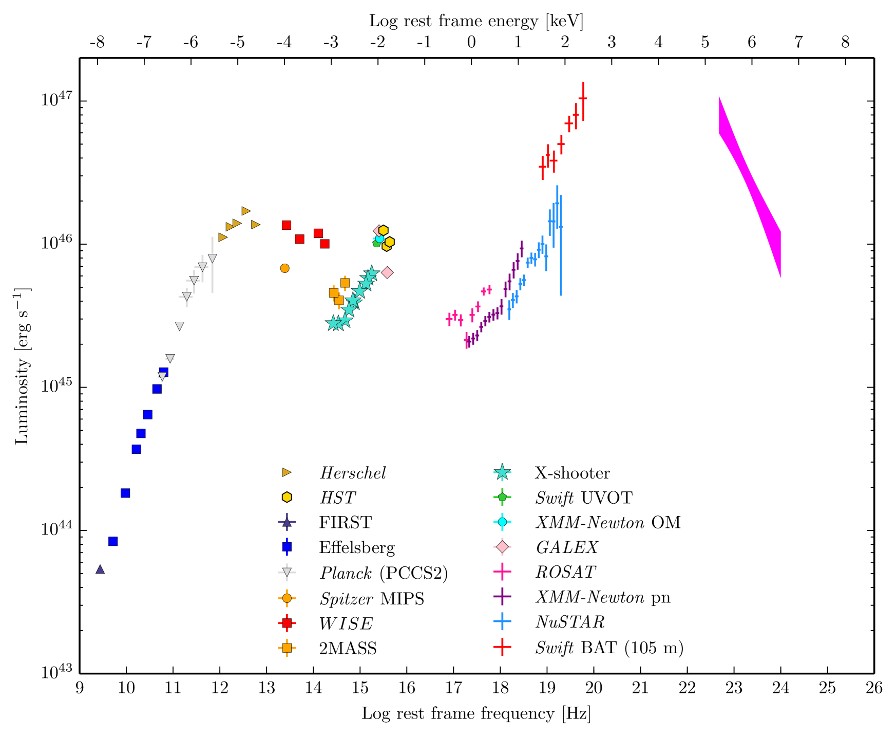
Figure 3: The multiwavelength SED of PKS J1222$+$0413. Our new data from Effelsberg (recorded between 2011 May and 2012 February), VLT X-shooter (recorded on 2017 April 3), NuSTAR and Swift (recorded on 2017 June 27) are shown with a Fermi $\gamma$-ray spectrum covering the same period as our new NIR/optical/UV/X-ray data (2017 March – July). We also show archival data from other facilities.

3.1.3 XMM-Newton

A short observation (12 ks) of PKS J1222$+$0413 was made by XMM-Newton on 2006 July 12. The observation data files (OBS ID: 0401790601) were obtained from the XMM-Newton Science Archive and reduced using the Science Analysis System (SAS, v16.0.0). The observation was strongly affected by background flaring, so after filtering the EPIC event files the good exposure times were 1.8, 3.8 and 3.6 ks for the pn, MOS1 and MOS2 detectors, respectively. Circular regions of radius $40^{\prime\prime}$ and $120^{\prime\prime}$ were used to extract the source and background spectra, respectively. The source extraction regions were centred on the source whereas the background extraction regions were placed on a blank patch of sky on the same chip as the source.

The XMM-Newton optical monitor (OM) observed PKS J1222$+$0413 using only the UVM2 filter. The photometry for this filter was extracted using the SAS omichain and omsource tasks and standard procedures.

Data analysis was performed with the X-ray spectral fitting package Xspec v12.9.0n (Arnaud 1996). We fitted all three EPIC (pn, MOS1 and MOS2) spectra simultaneously, allowing for a cross-normalisation factor between them; these did not vary by more than $\approx 6\%$. In all models we include a photoelectric absorption model (phabs) with the Galactic neutral hydrogen absorbing column set to the value $N_{\mathrm{H}}=1.66\times 10^{20}$ cm^-2 reported by Dickey & Lockman (1990) and adopting the elemental abundances of Wilms et al. (2000). The inclusion of an intrinsic absorber (zphabs) at the redshift of the source did not improve any of the fits. A broken power-law model is a statistically significant improvement over a single power-law, with an $F$-test probability greater than 99.99%. A more physical model including two Comptonisation regions, comptt (Titarchuk 1994) plus nthcomp (Życki et al. 1999) was no improvement over the simpler broken power-law. For the broken power-law model we determine an intrinsic flux of $(3.4\pm 0.1)\times 10^{-12}$ erg s^-1 cm^-2. The model parameters and fit results are summarised in Table 2 and the modelled spectra are shown in Figure 4.

Table 2: Results of XMM-Newton X-ray spectral fits

Model	Parameter	Value
powerlaw	$\Gamma$	$1.49\pm 0.03$
	norm.	$(3.6\pm 0.1)\times 10^{-4}$
	$\chi^{2}$/d.o.f.	179 / 134 = 1.34
bknpower	$\Gamma_{1}$	$1.65\pm 0.04$
	$E_{\mathrm{break}}$ [keV]	$2.4\pm 0.3$
	$\Gamma_{2}$	$1.1\pm 0.1$
	norm.	$(3.5\pm 0.1)\times 10^{-4}$
	$\chi^{2}$/d.o.f.	151 / 132 = 1.15
comptt +	$kT_{\mathrm{e}}$ [keV]	$0.7_{-0.1}^{+0.2}$
	$\tau$	$11_{-1}^{+2}$
	norm.	$\left(1.5_{-0.3}^{+0.5}\right)\times 10^{-2}$
nthcomp	$\Gamma$	$1.2\pm 0.1$
	norm.	$(1.5\pm 0.4)\times 10^{-4}$
	$\chi^{2}$/d.o.f.	151 / 131 = 1.16

Errors are quoted at the 1$\sigma$ level. All of the above models included a Galactic absorption component (phabs) with $N_{\mathrm{H}}=1.66\times 10^{20}$ cm^-2. The best-fit (broken power-law) model is plotted in Figure 4.

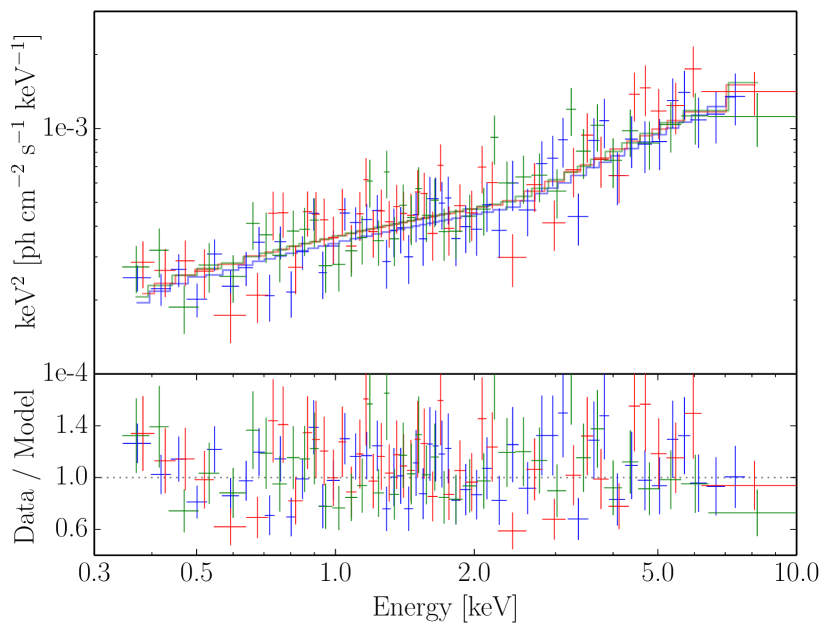
Figure 4: XMM-Newton EPIC X-ray spectra modelled with a broken power-law. Data from the pn, MOS1 and MOS2 detectors are shown in blue, red and green, respectively. The upper panel shows the data model with the detector responses folded out; the lower panel the data/model ratios.

3.1.4 Ly$\alpha$ contamination of photometry

The strong Ly$\upalpha$ ($\lambda_{\mathrm{rest}}=1216$ Å) line emission from the source appears at 2390 Å in the observed frame; it therefore contaminates the Swift UVOT UVW1, XMM-Newton OM UVM2 and GALEX NUV photometry. Precisely correcting for this contamination in this case is difficult since we have no measurement of the Ly$\upalpha$ EW and, as noted by Elvis et al. (2012), there is no (or weak) correlation between it and the EWs of either the Balmer lines or Mg ii. However, if we assume a typical Ly$\upalpha$ EW of 60 Å (in the rest frame), we can determine from the equations of Elvis et al. (2012) (their section 4.1.3) that Ly$\upalpha$ contributes approximately 20 per cent of the photometric flux.

3.1.5 Fermi

The Fermi $\gamma$-ray source 3FGL J1222.4$+$0414 is associated with PKS J1222$+$0413. In the Fermi LAT 4-year source catalogue (3FGL, Acero et al. 2015) the $\gamma$-ray source detection significance, derived from the test statistic (TS), is $30.01\sigma$. In the updated Fermi-LAT 8yr1 (FL8Y) description of the $\gamma$-ray sky with respect to 3FGL, the source significance improved slightly ($30.77\sigma$), and the spectral shape is described as a soft power-law with an index of $\Gamma=2.87\pm 0.04$, in the 100 MeV to 30 GeV energy range.

To construct a contemporaneous SED of PKS J1222$+$0413, we extracted $\gamma$-ray data from the period 2017 March 20–July 11 (to include our VLT X-shooter and NuSTAR observations) and from the period 2011 March–April (covering the HST COS UV spectrum of March 22 and SDSS optical spectrum of March 26). Photons in a circular region of interest (RoI) of radius 10^∘, centred on the position of PKS J1222$+$0413, were considered. A zenith-angle cut of 90^∘ was applied. The analysis was done using the Fermi Science Tools software package version v10r0p5, in combination with the PASS 8 instrument response functions (event class 128 and event type 3) corresponding to the P8R2_SOURCE_V6 response and the gll_iem_v06.fits and iso_P8R2_SOURCE_V6_v06 models for the Galactic and isotropic diffuse background, respectively. The spectral model of the region included all sources located within the RoI with spectral shapes and initial parameters as in the 3FGL catalogue (Acero et al. 2015).

The extraction of the Fermi-LAT data is complicated by the presence of two bright, nearby $\gamma$-ray sources in the RoI (see Figure 5). The prototypical quasar 3C 273 has an angular separation $\approx 2.7^{\circ}$ from PKS J1222$+$0413, comparable to the Fermi point spread function (PSF) at 1 GeV. Another quasar, PKS 1237$+$049, is $\approx 4.3^{\circ}$ from PKS J1222$+$0413. The Fermi PSF is larger at lower energies: the 95 per cent containment radius at 100 MeV is $\geqslant 10^{\circ}$.

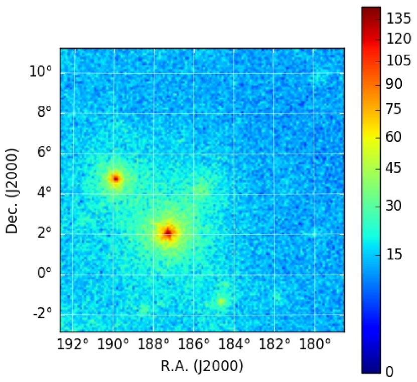
Figure 5: Fermi count map for the period beginning at the mission start and ending 2017 July 31. PKS J1222$+$0413 is at R.A. 185.59^∘, Dec. 4.22^∘. The brightest source in the field, 3C 273, is at R.A. 187.28^∘, Dec. 2.05^∘ and PKS 1237$+$049 (3FGL J1239.5$+$0443) is at R.A. 189.89^∘, Dec. 4.72^∘.

In the earlier time period (2011), PKS J1222$+$0413 is detected with a TS of 29.02 ($\approx 5.4\sigma$), the photon index being $\Gamma=2.72\pm 0.25$. The Fermi-LAT flux points at two bins/decade and the model spectrum up to the highest energy photon from the source in that period are shown in Figure 6, although we obtain a flux detection in one low-energy bin only. Note that $\gamma$-ray flux upper limits at the 95 per cent confidence level are computed for bins were TS < 9. In the 2017 time window, PKS J1222$+$0413 is detected with a TS of 56.68 ($\approx 7.5\sigma$), with a photon index of $\Gamma=2.74\pm 0.18$. The last significant enrgy bin is 1–3.16 GeV. We thus did not attempt any study of the variability, and note that in the Fermi All-Sky Variability Analysis (FAVA2) flare map of the region (generated in 2019 January using all available data from the mission start) that all of the flare activity is associated with other sources in the field (particularly 3C 273) and there are no recorded flare events in the vicinity of PKS J1222$+$0413. The spectral index found in both periods is fully compatible with the entire data set (FL8Y) within statistical errors (see Figure 6).

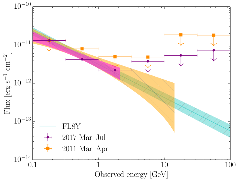
Figure 6: Fermi $\gamma$-ray spectra of PKS J1222$+$0413. The spectrum extracted from the period 2017 March 20 to July 11 is shown in fuchsia; the corresponding model is shown as the short (0.1–2 GeV) bow-tie. The spectrum extracted from the period 2011 March 1 to April 30 is shown in orange; the corresponding model is shown as the medium-length (0.1–14 GeV) bow-tie. For comparison, the model spectrum taken from the Fermi-LAT 8-year Source List (FL8Y) is shown as the long, turquoise bow-tie.

3.2 Radio monitoring data

3.2.1 Effelsberg

Observations were conducted with the 100 m Effelsberg telescope in Germany, with the secondary focus receivers at 2.64, 4.85, 8.35, 10.45, 14.6, 23.05 and 32 GHz. For the multiple-feed systems at 4.85, 10.45 and 32 GHz the measurements were conducted differentially thus removing most of the linear tropospheric effects. To correct for potential pointing offsets we have adopted the cross-scan technique; that is, register the telescope response while slewing its main beam over the expected source position. With our setup a complete radio SED needs roughly 40–45 minutes. It is therefore reasonable to assume that our observations are free of variability. Each pointing has been subjected to a pipeline of post-measurement corrections accounting for power losses caused by: (a) potential pointing offsets, (b) atmospheric absorption, and (c) deformations of the main telescope reflector. The fractional effect of each of these operations is given in Table 3 of Angelakis et al. (2019). The observed dataset has been finally calibrated with reference to standard sources listed in Table 3 of Angelakis et al. (2015). Table 3 in this paper summarises the flux densities at all observing frequencies weighted averaged over a period roughly from 2011 May 19 to 2012 February 18. The uncertainty in the average flux densities is limited to less that a couple of percent.

Table 3: Radio monitoring data from Effelsberg

Freq.	$\langle S\rangle$	$\sigma_{S}$	$N$	Start	Rate
(GHz)	(mJy)	(mJy)			(days)
2.64	663	3	9	2011-06-06	32.0
4.85	779	3	9	2011-05-19	34.3
8.35	923	5	10	2011-05-19	30.5
10.45	950	6	10	2011-05-19	30.5
14.60	920	10	10	2011-05-19	30.5
23.05	880	20	7	2011-05-19	45.7
32.00	830	20	6	2011-05-19	54.9

The error-weighted mean radio flux densities and their $1\sigma$ errors, the number of detections $N$ in the observation period starting on the given date and ending on 2012-02-18.

3.3 Additional archival data

3.3.1 FIRST

The Jansky Very Large Array (JVLA) Faint Images of the Radio Sky at Twenty centimetres (FIRST; Helfand et al. 2015) project surveyed 10575 square degrees of the sky at 1.4 GHz between 1993 and 2011. Querying the source catalogue, we find a radio source 0.5^′′ from the optical coordinates of PKS J1222$+$0413, which is the only radio source within a search radius of 30^′′. The integrated flux density was reported to be 800.63 mJy and we adopt an error of 5 per cent, representative of the systematic uncertaintiy for bright sources (White et al. 1997). The catalogue fluxes are measured in coadded images from multiple observations; the mean observation date is given as 2001 March 14 with an RMS of $\approx 4$ days.

3.3.2 Planck

ESA’s Planck space observatory (Tauber et al. 2010) operated from 2009 July, mapping the sky from high-frequency radio to far-infrared wavelengths. Its High-Frequency Instrument depleted its supply of liquid helium coolant in 2012 January, after which only the Low-Frequency Instrument (recording the 30, 44 and 70 GHz bands) was operable until the science mission ended in 2013 October.

We perform a cone search using the default radius equal to the beam FWHM at each frequency (see Planck Collaboration et al. 2016). In Table 4 we give the fluxes derived from the quoted catalogue flux densities which were calculated using the Gaussian fitting method. The source is not detected at 545 or 857 GHz either in the PCCS2 catalogue or the lower-reliability PCCS2E catalogue.

3.3.3 Herschel

The Herschel Space Observatory (Pilbratt et al. 2010) operated contemporaneously with Planck, from 2009 July to 2013 April. Herschel carried three science instruments: the Photodetecting Array Camera and Spectrometer (PACS, covering 55–220 $\upmu$m), the Spectral and Photometric Imaging Receiver (SPIRE, containing a low-resolution spectrometer covering 194–672 $\upmu$m and a photometer with three bands centred on 250, 350 and 500 $\upmu$m) and the Heterodyne Instrument for the Far Infrared (HIFI, covering 157–210 and 236–615 $\upmu$m). We searched the PACS and SPIRE point source catalogues (Marton et al. 2016; Marton et al. 2017) and obtained the data listed in Table 4.

3.3.4 Spitzer

PKS J1222$+$0413 has been observed by the Spitzer Space Telescope (Werner et al. 2004). The source was detected by the 24 $\upmu$m array of the the Multiband Imaging Photometer for Spitzer (MIPS) during an observation made on 28 January 2005. The source flux density is taken from the Spitzer Enhanced Imaging Products (SEIP) source list.

3.3.5 WISE

The Wide-field Infrared Survey Explorer (WISE; Wright et al. 2010) makes photometric observations in four bands: W1 (3.4 $\upmu$m), W2 (4.6 $\upmu$m), W3 (12 $\upmu$m) and W4 (22 $\upmu$m). For each band we have calculated the flux from the instrumental profile-fit photometry magnitude listed in the AllWISE catalogue. The magnitudes recorded for the bands were W1: $12.802\pm 0.023$; W2: $11.634\pm 0.023$; W3: $8.901\pm 0.034$ and W4: $6.513\pm 0.080$; the photometric quality of each band was reported to be of the highest quality.

The WISE telescope was placed into hibernation in 2011 February, following the depletion of its coolant. It was reactivated in 2013 September to begin the NEOWISE mission (Mainzer et al. 2014) using only the the two shortest-wavelength filters. Infrared photometry spanning several years is available for these filters, which sample the hot dust in our source. In Figure 7 we show the infrared lightcurves. Several exposures were taken on each pass of the telescope (with a cadence of roughly six months), which we have binned into the ten single-epoch measurements shown. For each epoch we have calculated the mean magnitude and its standard error from the individual exposures, after applying a $3\sigma$ clipping algorithm to remove anomalous data. The peak-to-peak magnitude change (from the first WISE observation in mid-2010 to the latest NEOWISE observation in mid-2017) is $\approx 1.2$ mag, and $\approx 0.6$ mag changes are seen in the NEOWISE period.

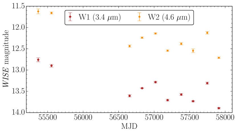
Figure 7: The WISE and NEOWISE infrared lightcurve of PKS J1222$+$0413, showing observations made between 2010 June and 2017 June.

3.3.6 2MASS

PKS J1222$+$0413 was detected as part of the Two Micron All Sky Survey (2MASS, Skrutskie et al. 2006), conducted between 1997 and 2001. The J, H and K_s profile-fit instrumental magnitudes recorded in the 2MASS All-Sky Point Source Catalog (PSC) were $16.348\pm 0.133$, $15.849\pm 0.146$ and $14.969\pm 0.140$, respectively.

3.3.7 Sloan

Two optical spectra of the source have been recorded as part of the Sloan Digital Sky Survey (SDSS). The first was taken on 12 February 2008 with the original SDSS spectrograph; the second was taken on 26 March 2011 with the Baryon Oscillation Spectroscopic Survey (BOSS) spectrograph, allowing a greater wavelength coverage. The two spectra are compared with our recent X-shooter spectrum in Figure 1. It can be seen that the 2011 spectrum is redder than that of 2008. Margala et al. (2016) noted that in the spectra of BOSS quasars, the flux densities were overestimated by $\sim 19$ per cent at 3300 Å and underestimated it by $\sim 24$ per cent at 1 $\upmu$m. Given the $\sim 1^{\prime\prime}$ seeing at 500 nm during our X-shooter observation, slit losses are likely minimal in the optical and UV, for which we used $1.2^{\prime\prime}$ and $1.3^{\prime\prime}$ width slits, respectively.

In the observed frame, the flux density at 4000 Å (7000 Å) is approximately 30 (25) per cent greater in the 2008 SDDS spectrum than in the 2017 X-shooter spectrum, and the flux densities of the two SDSS spectra are similar at 4000 Å.

3.3.8 GALEX

The Galaxy Evolution Explorer (GALEX; Martin et al. 2005), an ultraviolet space telescope, detected the source in both its near-ultraviolet (NUV) and far-ultraviolet (FUV) bands. The FUV flux is severely absorbed because the filter (1340–1806 Å) covers a spectral region blueward of the Lyman break of a Lyman limit system at 1793 Å (observed).

3.3.9 Hubble Space Telescope

Wotta et al. (2016) studied absorbing systems on sight lines towards 61 AGN, including PKS J1222$+$0413. As part of this study they obtained a short (900 s) exposure of the UV spectrum of the source using the G140L (900–2150 Å) filter of the HST Cosmic Origins Spectrograph (COS). This snapshot spectrum was recorded on 2011 March 22. They identified a Lyman limit system (LLS) with $\log(N_{\mathrm{H}})=17.55\pm 0.10$ cm^-2 at redshift $z_{\mathrm{LLS}}=0.6547$. The $N_{\mathrm{H}}$ was determined by assessing the suppression of continuum flux density relative to the composite quasar template of Telfer et al. (2002), scaled to match the unabsorbed region of the spectrum. We correct the observed spectrum for the Lyman continuum absorption by multiplying the fluxes by a factor $e^{\tau_{\lambda}}$ where the optical depth

$$\tau_{\lambda}=\sigma{\color[rgb]{0,0,0}{}_{0}}\left(\frac{\lambda}{\lambda_{\mathrm{LLS}}}\right)^{3}N_{\mathrm{H}}~{}~{}\mathrm{for}~{}~{}\lambda\leqslant\lambda_{\mathrm{LLS}},$$ (1)

the absorption cross-section at the Lyman limit $\sigma_{0}=6.3\times 10^{-18}$ cm² and $\lambda_{\mathrm{LLS}}=(1+z_{\mathrm{LLS}})\times 912$ Å  (Shull et al. 2017; Paresce 1984). The observed and corrected spectra are shown in Figure 8.

To estimate the AGN continuum, we select several regions free from narrow absorption lines and calculate the mean flux density in each of these and then bin into three wider regions, shown in Figure 8. It should be noted that the estimate of the column density of the LLS is dependent on the shape of the composite template used to approximate the intrinsic continuum. Without an independent measure of the column density, our ‘recovery’ of the PKS J1222$+$0413 AGN continuum is therefore also dependent on the shape of the template, so the flux density determined at 1370 Å should be treated with some caution. The continuum flux density at 1590 Å is perhaps slightly underestimated because of the intervening partial LLS at $z_{\mathrm{pLLS}}=0.89$, the column density of which is undetermined. The continuum flux density at 1860 Å is more reliable although all three estimates are hampered by the limited signal-to-noise of the spectrum. The spectrum blueward of $\approx 1100$ Å is too noisy to be of use.

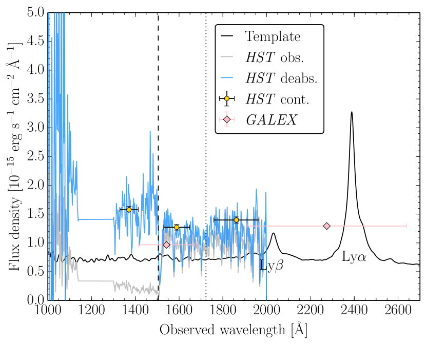
Figure 8: The HST COS spectrum of PKS J1222$+$0413. The observed spectrum is shown in grey. Overplotted in blue is the spectrum corrected for Galactic reddening and the Lyman continuum absorption of a Lyman limit system (LLS) at $z_{\mathrm{LLS}}=0.65$. The dashed vertical line indicates the Lyman break of the LLS; the dotted vertical line indicates the Lyman break of an intervening partial LLS at $z_{\mathrm{pLLS}}=0.89$. GALEX NUV and FUV photometry (corrected for Galactic reddening) are shown as pink diamonds. For reference, the composite spectrum of Telfer et al. (2002) is shown in black. This template has been scaled to approximately match the continuum flux level of the 2011 SDSS spectrum.

3.3.10 ROSAT

An 8 ks pointed observation of PKS  J1222$+$0413 was made by the Röntgensatellit (ROSAT; Voges et al. 1999) on 24 December 1992. The archival data was reduced using HEAsoft xselect v2.4d. The source extraction region was chosen to be a 120^′′-radius circle centred on the source. The background region was a 360^′′-radius circle offset on a blank patch of sky, on the same chip as the source. The 0.1–2.0 keV source count rate was $\approx 0.15$ counts s^-1. The source spectrum was rebinned using the grppha tool to contain a minimum of 20 counts per bin.

The best fitting model was a simple power-law with $\Gamma=1.72\pm 0.04$ and normalisation $(5.2\pm 0.2)\times 10^{-4}$, giving $\chi^{2}_{\nu}=90/57=1.58$. The best fit $N_{\mathrm{H}}=(7\pm 2)\times 10^{-3}$, lower than the Dickey & Lockman (1990) value but improving the fit by only $\Delta\chi^{2}=9$ for one additional free parameter.

3.3.11 Swift BAT

In the broad-band SED we also include data from the Swift Burst Alert Telescope (BAT) 105-month all-sky hard X-Ray survey (Oh et al. 2018) spanning the period 2004 December – 2013 August. The time-averaged spectrum and response file were obtained from the online archive. The spectrum was well-fit in Xspec with a single power-law of index $\Gamma=1.5\pm 0.1$ and normalisation $\left(9^{+5}_{-3}\right)\times 10^{-4}$, giving $\chi^{2}_{\nu}=0.32$.

Table 4: The multiwavelength data set

Q	Band	Instrument	Observation date	$\log(\nu_{\mathrm{obs}})$	Flux	Luminosity	Ref.
		(Survey)	(D/M/Y or M/Y)	[Hz]	[$10^{-14}$ erg/s/cm2]	[$10^{43}$ erg/s]
	Radio	(FIRST)	03/01	$9.15$	$1.12\pm 0.06$	$5.4\pm 0.3$	[1]
	Radio	Effelsberg	06/11–02/12	$9.42$	$1.750\pm 0.0008$	$8.40\pm 0.04$	[7]
	Radio	Effelsberg	05/11–02/12	$9.69$	$3.80\pm 0.01$	$18.3\pm 0.07$	[7]
	Radio	Effelsberg	05/11–02/12	$9.92$	$7.71\pm 0.04$	$37.0\pm 0.2$	[7]
	Radio	Effelsberg	05/11–02/12	$10.02$	$9.93\pm 0.06$	$47.7\pm 0.3$	[7]
	Radio	Effelsberg	05/11–02/12	$10.16$	$13.4\pm 0.2$	$64.5\pm 0.7$	[7]
	Radio	Effelsberg	05/11–02/12	$10.36$	$20.3\pm 0.5$	$97\pm 2$	[7]
	Radio	Planck	08/09–08/13	$10.48$	$25\pm 2$	$119\pm 9$	[2]
	Radio	Effelsberg	05/11–02/12	$10.51$	$26.6\pm 0.6$	$128\pm 3$	[7]
	Radio	Planck	08/09–08/13	$10.64$	$33\pm 2$	$158\pm 11$	[2]
	Radio	Planck	08/09–01/12	$10.85$	$55\pm 3$	$266\pm 16$	[2]
	Radio	Planck	08/09–01/12	$11.00$	$89\pm 14$	$429\pm 66$	[2]
	Radio	Planck	08/09–01/12	$11.16$	$116\pm 22$	$560\pm 100$	[2]
	Radio	Planck	08/09–01/12	$11.34$	$144\pm 31$	$690\pm 150$	[2]
	Radio	Planck	08/09–01/12	$11.55$	$165\pm 70$	$790\pm 340$	[2]
	Far-IR	Herschel	03/07/10	$11.78$	$233\pm 13$	$1117\pm 60$	[3]
	Far-IR	Herschel	03/07/10	$11.93$	$276\pm 14$	$1322\pm 67$	[3]
	Far-IR	Herschel	03/07/10	$12.08$	$292\pm 17$	$1399\pm 81$	[3]
	Far-IR	Herschel	03/07/10	$12.27$	$356\pm 41$	$1706\pm 200$	[3]
	Far-IR	Herschel	03/07/10	$12.48$	$285\pm 21$	$1369\pm 100$	[3]
	Far-IR	Spitzer MIPS	28/01/05	$13.11$	$142\pm 1$	$679\pm 6$	[4]
	Mid-IR	WISE	18–22/06/10	$13.13$	$283\pm 21$	$1358\pm 100$	[5]
	Mid-IR	WISE	18–22/06/10	$13.41$	$226\pm 7$	$1085\pm 34$	[5]
	Mid-IR	WISE	06/10–12/10	$13.81$	$248\pm 5$	$1191\pm 25$	[5]
	Mid-IR	WISE	06/10–12/10	$13.95$	$210\pm 4$	$1005\pm 21$	[5]
	Near-IR	(2MASS)	25/02/00	$14.14$	$95\pm 12$	$457\pm 59$	[6]
	Near-IR	(2MASS)	25/02/00	$14.26$	$84\pm 11$	$405\pm 55$	[6]
$\checkmark$	Near-IR	VLT X-shooter	03/04/17	$14.27$	$57.3\pm 0.5$	$275\pm 2$	[7]
	Near-IR	(2MASS)	25/02/00	$14.39$	$112\pm 14$	$536\pm 65$	[6]
$\checkmark$	Optical	VLT X-shooter	03/04/17	$14.48$	$74.2\pm 1.1$	$363\pm 5$	[7]
	Optical	(SDSS)	12/02/08	$14.48$	$124\pm 8$	$621\pm 40$	[8]
$\dagger$	Optical	(SDSS)	26/03/11	$14.48$	$122\pm 2$	$596\pm 10$	[9]
$\dagger$	UV	(SDSS)	26/03/11	$14.71$	$140\pm 7$	$699\pm 35$	[9]
$\checkmark$	UV	VLT X-shooter	03/04/17	$14.71$	$91.2\pm 0.6$	$513\pm 3$	[7]
$\checkmark$	UV	Swift UVOT	27/06/17	$15.06$	$211\pm 8$	$1011\pm 37$	[7]
	UV	XMM-Newton OM	12/07/06	$15.13$	$228\pm 4$	$1094\pm 19$	[7]
	UV	GALEX	31/03/04	$15.12$	$250\pm 8$	$1199\pm 38$	[10]
$\dagger$	UV	HST COS	22/03/11	$15.21$	$220\pm 20$	$1240\pm 90$	[7]
$\dagger$	UV	HST COS	22/03/11	$15.27$	$180\pm 20$	$1000\pm 100$	[7]
	UV	GALEX	31/03/04	$15.29$	$135\pm 16$	$649\pm 77$	[10]
$\dagger$	UV	HST COS	22/03/11	$15.35$	$30\pm 3$	$1040\pm 20$	[7]
	X-ray	ROSAT	24/12/92	$17.35$	$100\pm 9$	$500\pm 40$	[7]
$\checkmark$	X-ray	Swift XRT	27/06/17	$17.37$	$46\pm 12$	$230\pm 60$	[7]
	X-ray	XMM-Newton EPIC	12/07/06	$18.08$	$150\pm 8$	$720\pm 40$	[7]
$\checkmark$	X-ray	NuSTAR	27/06/17	$18.86$	$220\pm 10$	$1060\pm 50$	[7]
	X-ray	Swift BAT	12/04–09/10	$19.18$	$1450\pm 200$	$6960\pm 960$	[11]
$\checkmark$	$\gamma$-ray	Fermi LAT	03/17–06/17	$22.63$	$1300\pm 270$	$6300\pm 1300$	[7]
$\checkmark$	$\gamma$-ray	Fermi LAT	03/17–06/17	$23.13$	$420\pm 120$	$2020\pm 600$	[7]
$\checkmark$	$\gamma$-ray	Fermi LAT	03/17–06/17	$23.63$	$220\pm 100$	$1100\pm 470$	[7]
$\checkmark$	$\gamma$-ray	Fermi LAT	03/17–06/17	$24.13$	$<370$	$<1800$	[7]
$\checkmark$	$\gamma$-ray	Fermi LAT	03/17–06/17	$24.63$	$<530$	$<2600$	[7]
$\checkmark$	$\gamma$-ray	Fermi LAT	03/17–06/17	$25.13$	$<730$	$<3500$	[7]

References: [1] FIRST catalogue, Helfand et al. (2015); [2] Planck Second Point Source Catalog, Planck Collaboration et al. (2016); [3] Herschel point source catalogues, Marton et al. (2016); [4] Spitzer SEIP Source List, Werner et al. (2004); [5] WISE AllWISE Source Catalog, Wright et al. (2010); [6] Two Micron All-Sky Survey, Skrutskie et al. (2006); [7] this work; [8] Sloan Digital Sky Survey DR7, Abazajian et al. (2009); [9] Sloan Digital Sky Survey DR9, Ahn et al. (2012); [10] GALEX Data Release GR6, Martin et al. (2005); [11] Swift BAT 105-month all-sky hard X-Ray survey, Oh et al. (2018). The ‘Q’ flag indicates our quasi-simultaneous data ($\checkmark$ for data used in our SED fitting of Section 4.1.1 and $\dagger$ for optical/UV data used in Section 3.3.9).

4 The origin of the $\gamma$-ray emission

4.1 Determining the external photon field

Here, we determine the parameters of the ambient photon field with which the jet interacts to produce the observed high-energy emission. In the following we use our multiwavelength data to determine the size scales and luminosities of the accretion disc and its corona, the broad emission line region and the hot dusty torus. These are applied in our jet model which is described in Section 4.2.

4.1.1 The accretion flow

To model the infrared-to-X-ray SED we have scaled up the X-shooter fluxes by a factor 1.3 to match the level of the SDSS spectra in the UV (see § 3.3.7 and Figure 9). The Swift UVOT, XMM OM and GALEX NUV photometry have been scaled by a factor 0.8 to account for Ly$\upalpha$ contamination (see § 3.1.4). The XMM pn and ROSAT X-ray spectra have been scaled by factors 0.8 and 0.5, respectively, to match the flux level of our joint NuSTAR-Swift XRT observation. Note that the 2011 SDSS spectrum and HST COS spectrum (shown in lime green in Figure 9) were recorded three days apart.

We employ the energy-conserving accretion flow model, optxconv, of Done et al. (2013) and perform a simple test to determine whether the spin of the BH can be constrained by our data. In the optxconv model, a colour-temperature corrected accretion disc spectrum is produced from the accretion disc outer radius (which we set to the self-gravity radius) down to $R_{\mathrm{cor}}$, inside of which the accretion power is divided between warm and hot Comptonisation regions which are the origin of the observed soft X-ray excess and coronal power-law emission, respectively. As the BH spin increases, the innermost stable circular orbit moves closer to the BH and (for fixed $R_{\mathrm{cor}}$) this increases the emission from the Comptonisation regions. In this test we fix several parameters to those typical of a NLS1; namely, the warm Comptonisation region electron temperature $kT_{\mathrm{e}}{\color[rgb]{0,0,0}=0.2}$ keV and optical depth $\tau{\color[rgb]{0,0,0}=15}$, the photon index of the power-law tail $\Gamma{\color[rgb]{0,0,0}{}_{\mathrm{PL}}=2.4}$ and the ratio of power-law to soft excess power $f_{\mathrm{PL}}{\color[rgb]{0,0,0}=0.3}$. The outer accretion disc radius is fixed at 1000 $R_{\mathrm{g}}$.

As well as the accretion flow, we model the hot dust emission as simple blackbody, a scaled host galaxy template and add a power-law with $\Gamma=1.4$ to model the putative jet emission at hard X-ray energies. The hot dust temperature and luminosity is well determined by the WISE W1 and W2 points. The hot dust temperature is well-determined from the WISE W1 and W2 points and changes little between fits. As can be seen in Figure 9, our data do not strongly discriminate between zero- and high-spin models. However, the high-spin model slightly overpredicts the soft X-ray flux (although the modelled ROSAT spectrum has been scaled down by 20 per cent to match the flux level of the Swift XRT data) and cannot accommodate soft Comptonisation or coronal components. We note that this model conserves energy between the outer and inner accretion flow, producing the optical and UV/X-ray emission, respectively. The UV/X-ray flux would be lower if power were lost between outer and inner radii as the result of an accretion disc wind which could be present if the accretion rate were super-Eddington as in the high-spin model. We cannot therefore rule out a high BH spin. Overall, the zero-spin model is a better representation of the data and the parameters of the accretion flow components are then typical of a NLS1.

Table 5: Results from spectral fits to the deabsorbed IR to hard X-ray SED

	$a_{\star}$	$\nicefrac{{L}}{{L_{\mathrm{Edd}}}}$	$\dot{M}$	$R_{\mathrm{cor}}$	$\log(L_{\mathrm{AD}})$	$\log(L_{\mathrm{SX}})$	$\log(L_{\mathrm{PL}})$	$T_{\mathrm{tor}}$	$\log(L_{\mathrm{tor}})$	$R_{\mathrm{tor}}$	$\log(L_{\mathrm{AGN}})$	$\chi^{2}$/dof
			[$\nicefrac{{M$_{\sun}$}}{{yr}}$]	[$R_{\mathrm{g}}$]	[erg/s]	[erg/s]	[erg/s]	[K]	[erg/s]	[ld]	[erg/s]
	(1)	(2)	(3)	(4)	(5)	(6)	(7)	(8)	(9)	(10)	(11)	(12)
(a)	0.0	0.93	7.3	11.7	46.64	45.53	45.17	1430	46.19	4000	46.68	172/126
(b)	0.8	2.16	7.8	2.90	46.91	00.00	00.00	1350	46.21	4000	46.91	198/127

The columns are: (1) dimensionless BH spin: this was fixed at this value; (2) Eddington ratio; (3) mass accretion rate; (4) outer coronal radius in gravitational radii, $R_{\mathrm{g}}={\color[rgb]{0,0,0}2.95}\times 10^{11}$ m $={\color[rgb]{0,0,0}1.14}\times 10^{-2}$ light days; (5) luminosity of the accretion disc; (6) luminosity the soft Comptonisation region ‘SX’; (7) luminosity of the power-law tail ‘PL’; (8) temperature of the dusty torus; (9) luminosity of the IR radiation from the torus; (10) the dusty torus inner radius in light days; (11) the total AGN luminosity AD$+$SX$+$PL; (12) the $\chi^{2}$ statistic over the number of degrees of freedom (dof) in the model. $\dot{M}$ and $R_{\mathrm{tor}}$ are not model parameters but have been derived from our results.

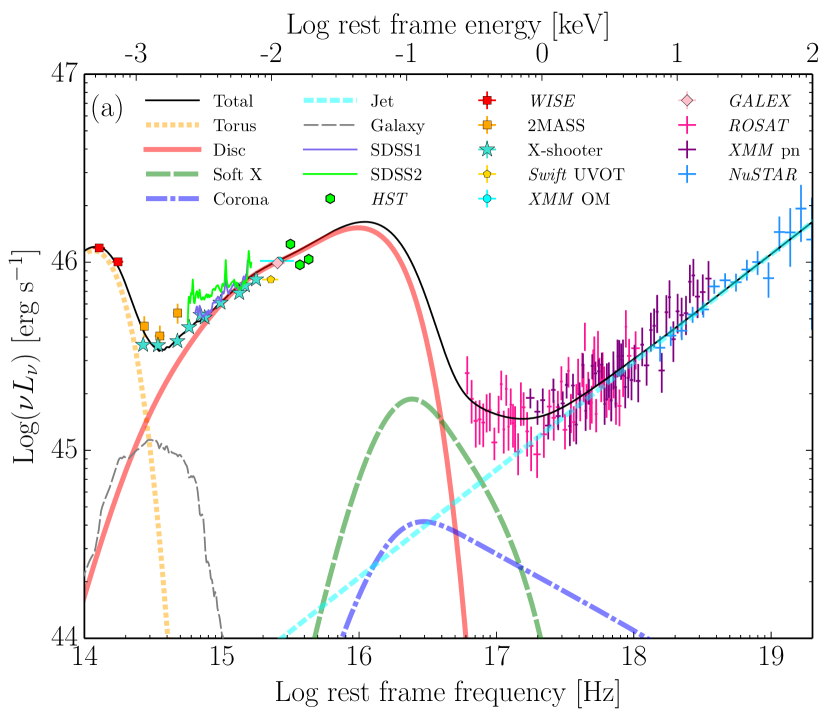
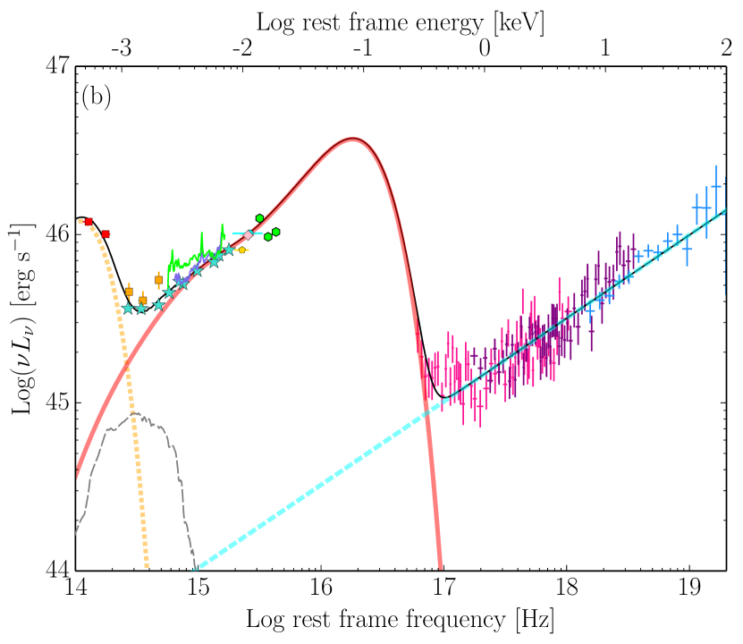
Figure 9: Accretion flow models applied to the NIR to X-ray SED, for different BH spins: (a) $a_{\star}=0$; (b) $a_{\star}=0.8$.

4.1.2 The broad line region luminosity and radius

The broad line region (BLR) is thought to be a system of gas clouds distributed on sub-parsec scales, very close to the central BH. The clouds are photoionised by the intense radiation from the accretion flow and the resulting line emission (and reflection) from the clouds can be Compton-scattered to higher energies by interaction with the particles in the relativistic jet.

Following the method described in Kynoch et al. (2018), we estimate the luminosity and radius of the BLR, from which the energy density of BLR photons can be calculated. Our X-shooter spectrum covers four of the prominent broad emission lines, (C iii], Mg ii, H$\upbeta$ and H$\upalpha$) from which we can estimate the BLR luminosity. The luminosities of the H$\upalpha$ and H$\upbeta$ broad components are listed in Table 1 and for the Mg ii line and C iii] broad components we get a luminosity of $\log L_{\rm MgII}=43.30$ erg s^-1 and $\log L_{\rm CIII]}=43.42$ erg s^-1, respectively. This results in a total BLR luminosity of $\log L_{\rm BLR}=44.54$ erg s^-1. As noted in Section 2.2, we estimate the BLR radius to be $260^{+91}_{-67}$ light-days ($\approx{\color[rgb]{0,0,0}2.28}\times 10^{4}~{}R_{\mathrm{g}}$ for our adopted BH mass) from the H$\upbeta$ radius-luminosity relationship of Bentz et al. (2013).

4.1.3 The dusty torus luminosity and radius

Photons from the extended ($\sim$parsec-scale) dusty torus are also upscattered by interaction with the jet. We parameterise this source of seed photons by the torus luminosity and radius (the latter is dependent on the dust temperature). The hot dust luminosity and temperature are determined from the blackbody fit to the mid-IR photometry: the values are listed in Table 5. Then, for a silicate dust composition, we estimate the hot dust radius to be $\sim 4000$ light-days ($\approx{\color[rgb]{0,0,0}3.51}\times 10^{5}~{}R_{\mathrm{g}}$). We note that the torus hot dust radius may be smaller than this depending on the assumption of grain size.

4.2 The broadband SED

We use the Gardner & Done (2018) single-zone, leptonic jet code jet (based on the physics of Ghisellini & Tavecchio 2009), adapted so that the external photon field can be set via input parameters. We first test the standard jet scalings against our data. For a BH of mass $M_{\mathrm{BH}}={\color[rgb]{0,0,0}2}\times 10^{8}$ M_☉ with $L/L_{\mathrm{Edd}}=\dot{m}={\color[rgb]{0,0,0}0.93}$, the scalings of Gardner & Done (2018) predict a magnetic field strength of $B\propto\sqrt{\dot{m}/M_{\mathrm{BH}}}={\color[rgb]{0,0,0}17.7}$ G and power injected into relativistic electrons $P_{\mathrm{rel}}\propto\dot{m}M_{\mathrm{BH}}={\color[rgb]{0,0,0}3.72}\times 10^{43}$ erg s^-1. Lengths scale linearly with mass, so in mass-normalised units the site of the jet emission region is equal to that of a typical Ghisellini et al. (2010) FSRQ, i.e. $Z_{\mathrm{diss}}=1280~{}R_{\mathrm{g}}$. For the jet geometry, we assume an opening angle $\phi=0.1$ radians and inclination to the line of sight equal to the inverse of the bulk Lorentz factor $i=1/\Gamma_{\mathrm{BLF}}$. We keep all other jet parameters equal to the mean FSRQ parameters of Ghisellini et al. (2010), listed under the “Scaled” model in Table 6, the resultant model is shown in Figure 10.

We find that the SED is not as discrepant as when performing the same test with 1H 0323$+$342 (see the top panels of Figure 10). The jet power $P_{\mathrm{j}}$ (relative to disc power) in this scaled model is comparable to other blazars but clearly the model needs some adjustment to fit the data.

We adjust the parameters of the scaled model to better fit the broadband SED. The Compton dominance (the ratio of peak Compton to synchrotron peak luminosities) of the scaled model is clearly too low; this can be increased by lowering $B$. The magnetic field is lowered approximately by a factor five in our fitted model compared to the scaled one. This is necessary in part to avoid the synchrotron self-Compton peak overpredicting the low-energy X-ray data. Increasing $P_{\mathrm{rel}}$ and $\Gamma_{\mathrm{BLF}}$ has the effect of increasing the jet SED in luminosity. A solution near equipartition (equal energy densities in electrons and the magnetic field) is found by adjusting $B$, $P_{\mathrm{rel}}$ and $\Gamma_{\mathrm{BLF}}$. By increasing $\Gamma_{\mathrm{BLF}}$, we can lower $P_{\mathrm{rel}}$ to reach approximate equipartition, having lowered $B$. Then, the shapes of the synchrotron and EC peaks are adjusted by tuning the parameters of the injected electron distribution (i.e. the low- and high-energy slopes $s_{1}$ and $s_{2}$ and the break Lorentz factor $\gamma_{\mathrm{brk}}$). It is necessary to lower $\gamma_{\mathrm{brk}}$ slightly to match the frequency peak of the synchrotron emission. The jet power in this fitted model is approximately half that of $L_{\mathrm{AD}}$.

It can be seen in Figure 10 that this fitted EC-disc model fits our broadband SED well. In particular we are able to achieve good agreement with our optical/UV data from X-shooter and Swift UVOT, soft X-ray data from NuSTAR and the Fermi $\gamma$-ray spectrum, all of which were obtained within the $\sim$three-month period 2017 March–June. However, this model does not fit the high-energy NuSTAR specrtum as well, although it is likely that the spectral shape above $\approx 20$ keV is not very well defined by the NuSTAR data. The harder jet X-ray spectrum in our model does match the Swift BAT spectrum taken from the 105-month monitoring campaign. The model also slightly overpredicts the mid-infrared data. This may be because we have not accounted for any synchrotron jet emission in the infrared in our modelling in Section 4.1.1. The mid-infrared variability seen in the WISE lightcurve (Figure 7) would suggest that the jet does make some contribution in this waveband. Any overestimation we may have made of the hot dust luminosity will have minimal impact on the models we have presented. This is because the jet emission region is closer to the accretion disc and BLR than the torus, therefore the energy density of infrared torus seed photons is relatively low.

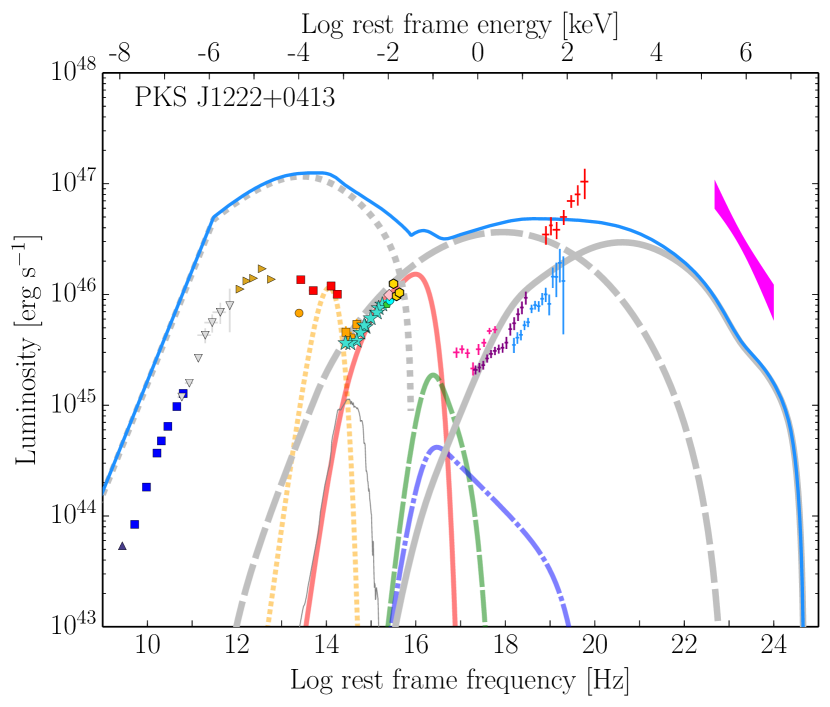
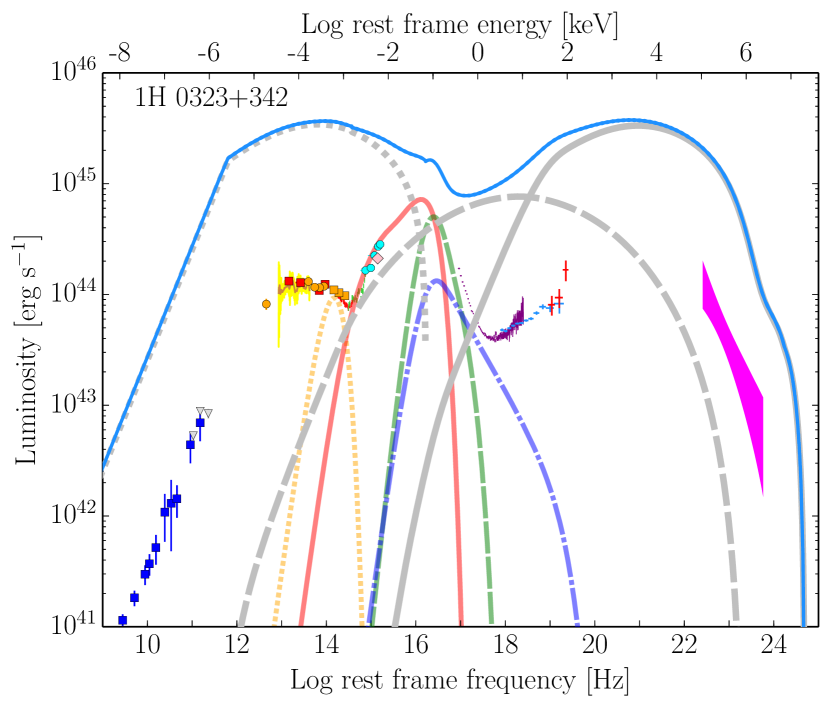
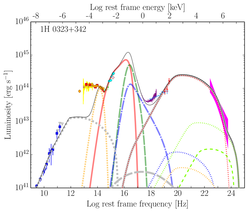
Figure 10: Top: Black hole mass and accretion rate scaled models of the jet emission from PKS J1222$+$0413 (left) and 1H 0323$+$342 (right). Bottom: Fitted EC-disc models for PKS J1222$+$0413 (left) and 1H 0323$+$342 (right). We show the three components of the jet emission (synchrotron, synchrotron self-Compton ‘SSC’ and external Compton ‘EC’) as grey lines. The individual EC components (from the disc, corona, BLR, reflection of the corona off the BLR ‘crf’ and torus) are shown as coloured dotted and dashed lines. The PKS J1222$+$0413 data are coded the same as Figure 3. The 1H 0323$+$342 models were presented by Kynoch et al. (2018).

Table 6: Jet parameters obtained from spectral fits to the full multiwavelength SED with bbody+optxconv+jet models

Parameter	Units	Model value
		PKS J1222$+$0413		1H 0323$+$342
		$\overbrace{\rule{99.58464pt}{0.0pt}}$		$\overbrace{\rule{99.58464pt}{0.0pt}}$
		Scaled with	EC-disc	Scaled with	EC-disc
		$M_{\mathrm{BH}}$ & $\dot{m}$		$M_{\mathrm{BH}}$ & $\dot{m}$
Input parameters:
$Z_{\mathrm{diss}}$	[$R_{\mathrm{g}}$] (ld)	1280 (15)	1280 (15)	1280 (1.5)	1280 (1.5)
$a_{\star}$		0.0	0.0	0.0	0.0
$i$	[deg]	4.41	2.86	4.41	4.77
$\Gamma_{\mathrm{BLF}}$		13	20	13	12
$\delta$		13	20	13	12
$B$	[G]	17.7	3.75	38	8
$\log(P_{\mathrm{rel}})$	[erg s-1]	43.6	42.9	42.24	41.0
$\gamma_{\mathrm{min}}$		1.00	1.00	1.00	1.00
$\gamma_{\mathrm{brk}}$		300	200	300	300
$\gamma_{\mathrm{max}}$		3000	3000	3000	3000
$s_{1}$		1.0	-1.0	1.0	1.5
$s_{2}$		2.7	3.2	2.7	2.7
Output / derived parameters:
$\gamma_{\mathrm{cool}}$		12	23	19	47
$\log(\nu_{\mathrm{ssa}})$	[Hz]	11.5	11.5	11.6	10.6
$\log\left(\nu_{\mathrm{peak}}^{\mathrm{sync}}\right)$	[Hz]	13.5	12.9	13.8	12.5
$\log\left(\nu L_{\nu_{\mathrm{peak}}}^{\mathrm{sync}}\right)$	[erg s-1]	47.1	46.2	45.56	43.12
$\log(P_{\mathrm{rad}})$	[erg s-1]	45.32	44.94	43.95	42.51
$\log(P_{\mathrm{e}})$	[erg s-1]	45.01	44.69	43.76	42.74
$\log(P_{B})$	[erg s-1]	45.45	44.48	44.12	42.70
$\log(P_{\mathrm{p}})$	[erg s-1]	47.28	46.31	45.91	45.01
$\log(P_{\mathrm{j}})$	[erg s-1]	47.30	46.35	45.93	45.01
$P_{\mathrm{j}}/L_{\mathrm{AD}}$		4.4	0.51	4.3	0.52
$U_{\mathrm{e}}/U_{B}$		0.37	1.6	0.44	1.1

Comparison of jet models for PKS J1222$+$0413 and the best fit model for 1H 0323$+$342 determined by Kynoch et al. (2018). $P_{\mathrm{rad}}$, $P_{\mathrm{e}}$, $P_{B}$, $P_{\mathrm{p}}$ and $P_{\mathrm{j}}$ are the radiative, electron, magnetic field, kinetic and total jet powers, respectively. $U_{\mathrm{e}}/U_{B}$ is the ratio of relativistic electron to magnetic field energy densities. The corresponding models are shown in Figure 10.

5 Discussion

5.1 PKS J1222$+$0413 as a NLS1

In Section 2.2 we found that the FWHM of the H$\upalpha$ and H$\upbeta$ Balmer lines and the individual lines of the Mg ii doublet are each lower than 2000 km s^-1, the limiting line width that is usually used to separate NLS1s from broad-line Seyferts (see Table 1). If, however, we use Gaussian rather than Lorentzian profiles to model the Mg ii lines, we determine FWHMs of 2240 km s^-1. Yao et al. (2015) found a similar $\mathrm{FWHM}=2264$ km s^-1 for H$\upbeta$ when modelling its broad component with a Gaussian. Torrealba et al. (2012) modelled the total Mg ii profile with two Gaussians (one broad and one narrow) centred at 2800 Å. For the broad component they determined a $\mathrm{FWHM}=5268$ km s^-1. Clearly, the determination of the emission line FWHMs (hence the classification of this source as either a narrow- or broad-line Seyfert 1) depends on the assumed line shape and the contribution of the narrow line component to the total line flux. Here, we have measured the Balmer line widths directly from their observed profiles, without assuming a particular line shape. In doing so, we have assumed that the flux contribution of the narrow line region is negligible, based on our estimation from a typical ratio of [O iii]$\lambda 5007$ to narrow H$\upbeta$ luminosities. If the narrow Balmer lines are somewhat stronger than we have estimated (which is possible, given the range of values of $L_{\mathrm{[O\textsc{iii}]}}/L^{\mathrm{n}}_{\mathrm{H}\upbeta}$ determined from large AGN samples) then the FWHMs of the broad Balmer would correspondingly increase to slightly above 2000 km s^-1. Alternative measures of the emission line FWHMs of this source may give values exceeding 2000 km s^-1, in which case PKS J1222$+$0413 is not strictly a NLS1. However, we point out that the 2000 km s^-1 limit is arbitrary and other authors have used more relaxed definitions of NLS1s (e.g. Zhou et al. 2006, Rakshit et al. 2017, Lakićević et al. 2018).

Czerny et al. (2018) emphasise that the 2000 km s^-1 division is a phenomenological one. The NLS1 definition of Osterbrock & Pogge (1985) was determined from low-mass objects in the local Universe. It has been proposed that NLS1s are objects that lie at the extreme of ‘Eigenvector 1’ (Boroson & Green 1992), with the sequence driven primarily by the accretion rate. A high accretion rate may be a better indicator of the high-mass, high-$z$ analogues of local NLS1s than the emission line FWHMs given that linewidths will be greater for higher-mass sources. Czerny et al. (2018) calculate that the dividing FWHM between narrow- and broad-line AGN is a factor $\approx 2$ greater in objects of a mass $3\times 10^{8}$ M_☉ than those of $10^{7}$ M_☉. Therefore for PKS J1222$+$0413, based on the BH mass the above scaling would imply a FWHM $\lesssim 4000$ km s^-1. Additionally, the strong Fe ii and weak [O iii] emission seen in the optical spectra are typical of NLS1s. We therefore confirm that PKS J1222$+$0413 is a NLS1, although one with a much greater than average mass.

The apparent weakness of the NLR is consistent with the view of this object as a high-luminosity, highly-accreting quasar. Netzer et al. (2004) suggested that the NLRs of high-luminosity AGN may be different to those of lower-luminosity, nearby sources. The NLR of high-luminosity sources may be lost as a result of being dynamically unbound. Collinson et al. (2017) found an anti-correlation between [O iii] $\lambda 5007$ line strength and Eddington ratio in their sample of high-redshift AGN. Several of their highest accretion rate sources had very weak [O iii] emission, similar to what we see in PKS J1222$+$0413. Based on their study of the super-Eddington NLS1 RX J0439.6$-$5311, Jin et al. (2017) present a picture of high accretion rate AGN which explains the weakness of the NLR as the result of it being (partly) shielded from the nuclear ionising flux by a ‘puffed up’ inner accretion disc or by a disc wind. Given the Eddington ratio determined for this source, it is unlikely that PKS J1222$+$0413 has a super-Eddington wind like RX J0439.6$-$5311. However, its SED peaks in the FUV and the accretion flow X-ray spectrum is very soft and would therefore not over-ionise material driven out in a UV line-driven wind. It may be that PKS J1222$+$0413 has a UV line-driven wind partly shielding the NLR. Although the narrow emission lines are weak, we find that the high-ionisation lines (emitted by gas between the BLR and NLR) are strong, e.g. Neon ([Ne iv]$\lambda 2423$) and the Iron transitions (Fe xi).

5.2 The jet of PKS J1222$+$0413

It was challenging to extract the $\gamma$-ray spectrum of PKS J1222$+$0413 (Section 3.1.5). Because of the close proximity of the bright $\gamma$-ray sources 3C 273 and PKS 1237$+$049 we found that very few photons in the field had a strong statistical association with PKS J1222$+$0413; most were more favourably associated with the other sources. Applying an 85 per cent confidence cut, we are left with very few photons and a limited $\gamma$-ray spectrum. As we noted earlier, there have been no $\gamma$-ray flares recorded by Fermi near the location of PKS J1222$+$0413. Rapid variability in the optical has not been recorded either, with Ojha et al. (2018) noting that the intra-night optical variability was remarkably low, and consistent with levels see in non-jetted (radio-quiet) sources. However, the WISE data (Figure 7) show variability which is likely from jet synchrotron emission.

Whereas the viewing angle to the jet (and hence the bulk Lorentz and Doppler factors, under the assumption $i=1/\Gamma_{\mathrm{BLF}}\approx\delta$) was constrained by radio measurements (Fuhrmann et al. 2016) in the case of 1H 0323$+$342 (Kynoch et al. 2018), we have no such observational constraint for the jet of PKS J1222$+$0413. Lister et al. (2016) investigated the radio jet of PKS J1222$+$0413 as part of the MOJAVE project and found that the jet is two-sided on kpc scales (but it is one-sided on pc scales). Lister (2018) notes that no measurable motion within the jet has been recorded in a 14-year monitoring period and that the maximum apparent jet speed is sub-luminal: $(0.9\pm 0.3)c$. If the transverse speed of the jet $v_{\mathrm{t}}=0.9c$, this would imply a large viewing angle to the jet axis with $i\approx 50$–90^∘ and a low bulk Lorentz factor whereas high Lorentz factors are determined by SED modelling (e.g. Yao et al. 2015). The viewing angle is likely to be small because of the one-sided pc-scale jet structure. Its long-term (2008 to date) 15 GHz radio lightcurve, recorded by the Owens Valley Radio Observatory (OVRO, Richards et al. 2011), shows variability which is also suggestive of a high Doppler factor and low viewing angle. It is likely that the apparent sub-luminal motion is due to a lack of traceable bright knots, rather than a low-speed jet.

Whilst it is difficult to extract a reliable $\gamma$-ray spectrum for PKS J1222$+$0413 because of its low $\gamma$-ray flux and the presence of bright nearby sources, we are confident of the $\gamma$-ray nature of our source. Other, well-defined properties such as the radio and infrared variability and high-resolution radio images of the jet are supportive of the presence of very high energy processes. Furthermore, the X-ray data from NuSTAR and Swift BAT are evidence of a high-energy Compton component, and the $\gamma$-ray spectrum appears to be consistent with the very high-energy tail of this feature.

5.3 Comparison with 1H 0323$+$342

We presented a very similar analysis of the lowest-redshift $\gamma$-NLS1, 1H 0323$+$342, in Kynoch et al. (2018). Here we make a comparison with our findings from PKS J1222$+$0413. Obviously, PKS J1222$+$0413 has a much greater BH mass than 1H 0323$+$342. We therefore expect PKS J1222$+$0413 to be more similar to a standard (high-mass) blazar. Indeed, when we scale a standard FSRQ jet by mass and mass accretion rate we see that discrepancy between the predicted SED and the data is much less than Kynoch et al. (2018) found for 1H 0323$+$342. The high accretion rate of PKS J1222$+$0413 means that a high magnetic field is predicted from the scaling relations. As with 1H 0323$+$342, the resultant predicted SED has a low Compton dominance and a shape much more akin to a BL Lac, albeit at a much higher luminosity than BL Lacs. We can better fit the data by turning down the magnetic field strength. (With 1H 0323$+$342 it was necessary to turn down both the magnetic field strength and the power injected into the relativistic electrons.) As with 1H 0323$+$342, a typical NLS1 SED model fits the observed NIR–X-ray SED well, if a (jet) power-law is added to account for hard X-rays. In 1H 0323$+$342 Kynoch et al. (2018) found that the X-ray photon index below $\approx 2$ keV was very soft, typical of (non-jetted) NLS1s, whereas above 2 keV, the photon index was much harder, typical of nonthermal jet emission. This was interpreted as a transition from accretion-flow-dominated to jet-dominated emission. We do not find such strong evidence of a soft, low-energy photon index in PKS J1222$+$0413 (Sections 3.1.3 and 4.1.1), likely because its higher mass and redshift mean that the accretion flow makes less of a contribution to the flux in the XMM-Newton bandpass.

Kynoch et al. (2018) showed that 1H 0323$+$342 had a low jet power for its accretion power, compared to the Fermi blazars studied by Ghisellini et al. (2014). Here, we find that the jet of PKS J1222$+$0413 is similarly underpowered relative to its accretion power. However, since it has a BH mass similar to FSRQs, in terms of its absolute jet power it occupies the same region of the blazar sequence as the FSRQs, as one might expect. Foschini (2017) proposed that there are two branches on the blazar sequence. This can be seen if the jet power (calculated from the radio luminosity) is plotted against the disc luminosity. The track of the main branch, containing FSRQs and BL Lacs (which have similar BH masses), may be explained as a difference in the environment in which the relativistic electrons cool. The lower track, connecting radio-loud NLS1s to FSRQs (which have similar cooling environments), must be driven by the difference in the BH masses. A small number of sources have jet powers estimated both from their radio luminosity and from SED modelling. We find that the jet power calculated via SED modelling is generally greater than that estimated from the radio luminosity. Paliya et al. (2019) have modelled the broadband SEDs of sixteen $\gamma$-NLS1s to determine the jet powers, and have compared these to a sample of previously-modelled blazars. Their results suggest that $\gamma$-NLS1s form the low-jet-power tail of the FSRQ population, rather than forming a separate branch.

Yao et al. (2015) also modelled the SED of PKS J1222$+$0413 and presented both an EC-BLR and EC-torus case in which the $\gamma$-rays were predominantly upscattered seed photons from the BLR or torus, respectively. Here, we have demonstrated that an EC-disc model can also reproduce the observed SED. In our EC-disc model we determine a high bulk Lorentz factor $\Gamma_{\mathrm{BLF}}=20$, which is substantially greater than the mean value 13 Ghisellini et al. (2010) found for FSRQs and the value 12 Kynoch et al. (2018) found for 1H 0323$+$342. The factors determined by Yao et al. (2015) from their jet models were even higher: $\Gamma_{\mathrm{BLF}}=26$, 35 for the EC-BLR and EC-torus models, respectively. Unfortunately, Yao et al. (2015) do not quote any jet powers determined from their models, or give sufficient details of their model parameters and so it is not possible to undertake a meaningful comparison. We emphasise that the jet power and parameters determined by SED fitting are still model-dependent. The results which are obtained will depend on the detailed assumptions made, and the approaches taken to compute the complex physical processes. Even within the same prescription, the complexity of jet models mean that it is difficult to converge on a unique solution. Our approach has been to construct a quasi-simultaneous data set and to self-consistently model and apply the ambient photon field which is crucial in reproducing the observed external Compton (X-ray and $\gamma$-ray) emission. In future studies it would be useful if the results were presented in a more uniform way, with equivalent model parameters and basic assumptions stated.

6 Conclusions

Our main results are summarised below:

• The BH mass ${\color[rgb]{0,0,0}\approx 2}\times 10^{8}$ M_☉ is very high for a NLS1, which typically have an order of magnitude smaller BH masses.

• We conclude that PKS J1222$+$0413 is a NLS1, based on our new data and analysis of its optical spectral properties and the accretion flow parameters obtained from modelling its broadband SED. This is in agreement with the NLS1 classification made by Yao et al. (2015).

• The very weak [O iii] is suggestive of a UV line-driven disc wind shielding the narrow-line region from ionising UV flux produced near to the BH.

• The jet power is approximately half of the accretion disc luminosity whereas for BL Lac and FSRQ-type blazars, the jet power typically exceeds the accretion power (Ghisellini et al. 2014). This finding is similar to the result for the $\gamma$-NLS1 1H 0323$+$342 which Kynoch et al. (2018) also found to have an underpowered jet.

• Because of its high BH mass, similar to FSRQ-type blazars, PKS J1222$+$0413 lies in the region of the blazar sequence occupied by the FSRQs. Most other $\gamma$-ray detected NLS1s, like 1H 0323$+$342, have much lower absolute jet powers (similar to BL Lacs) but share many of the same jet properties as FSRQs. PKS J1222$+$0413 is therefore an ideal object in which to explore the relationship between $\gamma$-NLS1s and FSRQs.

References

- Abazajian et al. (2009) Abazajian K. N., et al., 2009, ApJS, 182, 543
- Abdo et al. (2009) Abdo A. A., et al., 2009, ApJ, 707, L142
- Acero et al. (2015) Acero F., et al., 2015, ApJS, 218, 23
- Ahn et al. (2012) Ahn C. P., et al., 2012, ApJS, 203, 21
- Angelakis et al. (2015) Angelakis E., et al., 2015, A&A, 575, A55
- Angelakis et al. (2019) Angelakis E., et al., 2019, arXiv e-prints,
- Arnaud (1996) Arnaud K. A., 1996, in Jacoby G. H., Barnes J., eds, Astronomical Society of the Pacific Conference Series Vol. 101, Astronomical Data Analysis Software and Systems V. p. 17
- Bentz et al. (2013) Bentz M. C., et al., 2013, ApJ, 767, 149
- Blackburn (1995) Blackburn J. K., 1995, in Shaw R. A., Payne H. E., Hayes J. J. E., eds, Astronomical Society of the Pacific Conference Series Vol. 77, Astronomical Data Analysis Software and Systems IV. p. 367
- Blandford & Znajek (1977) Blandford R. D., Znajek R. L., 1977, MNRAS, 179, 433
- Boroson & Green (1992) Boroson T. A., Green R. F., 1992, ApJS, 80, 109
- Capellupo et al. (2015) Capellupo D. M., Netzer H., Lira P., Trakhtenbrot B., Mejía-Restrepo J., 2015, MNRAS, 446, 3427
- Cohen (1983) Cohen R. D., 1983, ApJ, 273, 489
- Collinson et al. (2017) Collinson J. S., Ward M. J., Landt H., Done C., Elvis M., McDowell J. C., 2017, MNRAS, 465, 358
- Cushing et al. (2004) Cushing M. C., Vacca W. D., Rayner J. T., 2004, PASP, 116, 362
- Czerny et al. (2018) Czerny B., Panda S., Śniegowska M., Kozlowski S., Nikolajuk M., Du P., You B., 2018, in Revisiting narrow-line Seyfert 1 galaxies and their place in the Universe. 9-13 April 2018. Padova Botanical Garden, Italy. p. 30 (arXiv:1806.06741)
- Dickey & Lockman (1990) Dickey J. M., Lockman F. J., 1990, ARA&A, 28, 215
- Done et al. (2013) Done C., Jin C., Middleton M., Ward M., 2013, MNRAS, 434, 1955
- Elvis et al. (2012) Elvis M., et al., 2012, ApJ, 759, 6
- Foschini (2017) Foschini L., 2017, Frontiers in Astronomy and Space Sciences, 4, 6
- Fossati et al. (1998) Fossati G., Maraschi L., Celotti A., Comastri A., Ghisellini G., 1998, MNRAS, 299, 433
- Freudling et al. (2013) Freudling W., Romaniello M., Bramich D. M., Ballester P., Forchi V., García-Dabló C. E., Moehler S., Neeser M. J., 2013, A&A, 559, A96
- Fuhrmann et al. (2016) Fuhrmann L., et al., 2016, Research in Astronomy and Astrophysics, 16, 176
- Gardner & Done (2014) Gardner E., Done C., 2014, MNRAS, 438, 779
- Gardner & Done (2018) Gardner E., Done C., 2018, MNRAS, 473, 2639
- Ghisellini & Tavecchio (2009) Ghisellini G., Tavecchio F., 2009, MNRAS, 397, 985
- Ghisellini et al. (2010) Ghisellini G., Tavecchio F., Foschini L., Ghirlanda G., Maraschi L., Celotti A., 2010, MNRAS, 402, 497
- Ghisellini et al. (2014) Ghisellini G., Tavecchio F., Maraschi L., Celotti A., Sbarrato T., 2014, Nature, 515, 376
- Ghisellini et al. (2017) Ghisellini G., Righi C., Costamante L., Tavecchio F., 2017, MNRAS, 469, 255
- Giommi et al. (2012) Giommi P., et al., 2012, A&A, 541, A160
- Greene et al. (2010) Greene J. E., et al., 2010, ApJ, 723, 409
- Harrison et al. (2013) Harrison F. A., et al., 2013, ApJ, 770, 103
- Helfand et al. (2015) Helfand D. J., White R. L., Becker R. H., 2015, ApJ, 801, 26
- Jin et al. (2017) Jin C., Done C., Ward M., Gardner E., 2017, MNRAS, 471, 706
- Kalberla et al. (2005) Kalberla P. M. W., Burton W. B., Hartmann D., Arnal E. M., Bajaja E., Morras R., Pöppel W. G. L., 2005, A&A, 440, 775
- Kynoch et al. (2018) Kynoch D., et al., 2018, MNRAS, 475, 404
- Lakićević et al. (2018) Lakićević M., Popović L. Č., Kovačević-Dojčinović J., 2018, MNRAS, 478, 4068
- Landt et al. (2017) Landt H., et al., 2017, MNRAS, 464, 2565
- Larsson et al. (2018) Larsson J., D’Ammando F., Falocco S., Giroletti M., Orienti M., Piconcelli E., Righini S., 2018, MNRAS, 476, 43
- Lister (2018) Lister M., 2018, in Revisiting narrow-line Seyfert 1 galaxies and their place in the Universe. 9-13 April 2018. Padova Botanical Garden, Italy. p. 22 (arXiv:1805.05258)
- Lister et al. (2016) Lister M. L., et al., 2016, AJ, 152, 12
- Mainzer et al. (2014) Mainzer A., et al., 2014, ApJ, 792, 30
- Margala et al. (2016) Margala D., Kirkby D., Dawson K., Bailey S., Blanton M., Schneider D. P., 2016, ApJ, 831, 157
- Martin et al. (2005) Martin D. C., et al., 2005, ApJ, 619, L1
- Marton et al. (2016) Marton G., et al., 2016, in Jablonka P., André P., van der Tak F., eds, IAU Symposium Vol. 315, From Interstellar Clouds to Star-Forming Galaxies: Universal Processes?. p. E53 (arXiv:1510.08325), doi:10.1017/S1743921316008152
- Marton et al. (2017) Marton G., et al., 2017, preprint, (arXiv:1705.05693)
- Mejía-Restrepo et al. (2016) Mejía-Restrepo J. E., Trakhtenbrot B., Lira P., Netzer H., Capellupo D. M., 2016, MNRAS, 460, 187
- Netzer et al. (2004) Netzer H., Shemmer O., Maiolino R., Oliva E., Croom S., Corbett E., di Fabrizio L., 2004, ApJ, 614, 558
- Oh et al. (2018) Oh K., et al., 2018, ApJS, 235, 4
- Ojha et al. (2018) Ojha V., Krishna G., Chand H., 2018, MNRAS,
- Onken et al. (2004) Onken C. A., Ferrarese L., Merritt D., Peterson B. M., Pogge R. W., Vestergaard M., Wandel A., 2004, ApJ, 615, 645
- Osterbrock & Pogge (1985) Osterbrock D. E., Pogge R. W., 1985, ApJ, 297, 166
- Paliya et al. (2019) Paliya V. S., Parker M. L., Jiang J., Fabian A. C., Brenneman L., Ajello M., Hartmann D., 2019, ApJ, 872, 169
- Paresce (1984) Paresce F., 1984, in Kondo Y., Bruhweiler F. C., Savage B. D., eds, NASA Conference Publication Vol. 2345, NASA Conference Publication.
- Pilbratt et al. (2010) Pilbratt G. L., et al., 2010, A&A, 518, L1
- Planck Collaboration et al. (2016) Planck Collaboration et al., 2016, A&A, 594, A26
- Polletta et al. (2007) Polletta M., et al., 2007, ApJ, 663, 81
- Rakshit et al. (2017) Rakshit S., Stalin C. S., Chand H., Zhang X.-G., 2017, ApJS, 229, 39
- Richards et al. (2011) Richards J. L., et al., 2011, ApJS, 194, 29
- Shull et al. (2017) Shull J. M., Danforth C. W., Tilton E. M., Moloney J., Stevans M. L., 2017, ApJ, 849, 106
- Sikora & Begelman (2013) Sikora M., Begelman M. C., 2013, ApJ, 764, L24
- Skrutskie et al. (2006) Skrutskie M. F., et al., 2006, AJ, 131, 1163
- Tauber et al. (2010) Tauber J. A., et al., 2010, A&A, 520, A1
- Telfer et al. (2002) Telfer R. C., Zheng W., Kriss G. A., Davidsen A. F., 2002, ApJ, 565, 773
- Titarchuk (1994) Titarchuk L., 1994, ApJ, 434, 570
- Torrealba et al. (2012) Torrealba J., Chavushyan V., Cruz-González I., Arshakian T. G., Bertone E., Rosa-González D., 2012, Rev. Mex. Astron. Astrofis., 48, 9
- Vacca et al. (2003) Vacca W. D., Cushing M. C., Rayner J. T., 2003, PASP, 115, 389
- Vernet et al. (2011) Vernet J., et al., 2011, A&A, 536, A105
- Véron-Cetty et al. (2001) Véron-Cetty M.-P., Véron P., Gonçalves A. C., 2001, A&A, 372, 730
- Voges et al. (1999) Voges W., et al., 1999, A&A, 349, 389
- Werner et al. (2004) Werner M. W., et al., 2004, ApJS, 154, 1
- White et al. (1997) White R. L., Becker R. H., Helfand D. J., Gregg M. D., 1997, ApJ, 475, 479
- Wilms et al. (2000) Wilms J., Allen A., McCray R., 2000, ApJ, 542, 914
- Wotta et al. (2016) Wotta C. B., Lehner N., Howk J. C., O’Meara J. M., Prochaska J. X., 2016, ApJ, 831, 95
- Wright (2006) Wright E. L., 2006, PASP, 118, 1711
- Wright et al. (2010) Wright E. L., et al., 2010, AJ, 140, 1868
- Yao et al. (2015) Yao S., Yuan W., Zhou H., Komossa S., Zhang J., Qiao E., Liu B., 2015, MNRAS, 454, L16
- Zhou et al. (2006) Zhou H., Wang T., Yuan W., Lu H., Dong X., Wang J., Lu Y., 2006, ApJS, 166, 128
- Życki et al. (1999) Życki P. T., Done C., Smith D. A., 1999, MNRAS, 309, 561