The complex life of hydrodynamic modes

Abstract

We study analytic properties of the dispersion relations in classical hydrodynamics by treating them as Puiseux series in complex momentum. The radii of convergence of the series are determined by the critical points of the associated complex spectral curves. For theories that admit a dual gravitational description through holography, the critical points correspond to level-crossings in the quasinormal spectrum of the dual black hole. We illustrate these methods in ${\cal N}=4$ supersymmetric Yang-Mills theory in 3+1 dimensions, in a holographic model with broken translation symmetry in 2+1 dimensions, and in conformal field theory in 1+1 dimensions. We comment on the pole-skipping phenomenon in thermal correlation functions, and show that it is not specific to energy density correlations.

1 Introduction

Hydrodynamics is an effective theory of fluids valid at sufficiently long times and sufficiently large distances. Classical hydrodynamics is formulated by combining conservation laws for energy, momentum, and other charges (such as the particle number in non-relativistic systems) with the constitutive relations expressing the conserved fluxes in terms of the hydrodynamic variables: local temperature, fluid velocity, and charge density landau . The constitutive relations are written down on the basis of symmetry, using the derivative expansion. The constitutive relations which contain no derivatives of the hydrodynamic variables are said to describe “perfect fluids”, corresponding to “zeroth-order” hydrodynamics. The constitutive relations which contain up to one derivative of the hydrodynamic variables are commonly said to describe “viscous fluids”, corresponding to “first-order” or “Navier-Stokes” hydrodynamics. One can proceed by adding terms with more derivatives of the hydrodynamic variables to the constitutive relations, hoping to improve the hydrodynamic description of the actual physical fluids. The constitutive relations which contain up to $n$ derivatives of the hydrodynamic variables then give rise to $n^{\rm th}$-order hydrodynamics. In this paper, we will use simple facts from the theory of complex curves in order to study some aspects of convergence of the above derivative expansion. Our focus will be on relativistic fluids, and we shall illustrate general results with the examples of strongly interacting quantum field theories possessing a dual holographic description.

A neutral homogeneous and isotropic relativistic fluid whose energy-momentum tensor is conserved supports collective excitations in the form of shear and sound hydrodynamic modes Kovtun:2012rj . The collective modes arise from the analysis of linearised fluctuations of energy and momentum densities around the equilibrium state at temperature $T$. The mode’s frequency $\omega$ is related to the wave vector ${\bf q}$ by the dispersion relation $\omega=\omega({\bf q})$. In hydrodynamics, the dispersion relations are given by

Shear mode: $$\omega_{\rm shear}({\bf q})=-iD{\bf q}^{2}+\cdots\,,$$ (1)

Sound mode: $$\omega_{\rm sound}^{\pm}({\bf q})=\pm v_{s}|{\bf q}|-i\frac{\Gamma_{\!s}}{2}\,{\bf q}^{2}+\cdots\,,$$ (2)

where $v_{s}$ is the speed of sound, and $D$ and $\Gamma_{\!s}$ can be expressed through relevant transport coefficients. In $d_{s}$ spatial dimensions, we have

$$D=\frac{\eta}{\epsilon+p}\,,$$ (3)

$$\Gamma_{\!s}=\frac{1}{\epsilon+p}\left[\zeta+\frac{2d_{s}-2}{d_{s}}\,\eta\right],$$ (4)

where $\epsilon$ and $p$ are the equilibrium energy density and pressure, and $\eta$ and $\zeta$ are the shear and bulk viscosities. The shear mode (1) describes diffusion of the transverse (to the wave vector) velocity fluctuations which are damped by the shear viscosity. The sound mode (2) describes propagation of the longitudinal velocity fluctuations together with the fluctuations in the energy density and pressure. The terms written down in (1) and (2) represent the contributions from first-order hydrodynamics, while the ellipses denote terms with higher powers of ${\bf q}$, which can be matched to transport coefficients in second- and higher-order hydrodynamics Baier:2007ix ; Bhattacharyya:2012nq ; Grozdanov:2015kqa . To all orders in the hydrodynamic derivative expansion, the dispersion relations (1), (2) are represented by infinite series in ${\bf q}$.

Are these hydrodynamic series convergent? If so, what are their radii of convergence and what determines them? If the series are only asymptotic, can they be resummed? The shear mode (1) appears to be an expansion in powers of ${\bf q}^{2}$, whereas the sound mode (2) seems to contain odd and even powers of $|{\bf q}|=\sqrt{{\bf q}^{2}}$ in its real and imaginary part, respectively. Can we prove that no other power of ${\bf q}^{2}$ or non-analytic terms appears in the hydrodynamic expansions at any order? These questions were considered in our recent short paper Grozdanov:2019kge , and we shall provide more details here.

In general, proving convergence of a perturbative series and finding the corresponding radius of convergence may constitute rather difficult (and rather different) problems. For example, the convergence of the so called $1/Z$ series representing the lowest energy eigenvalue of the two-electron atom with the nucleus of charge $Z$ was rigorously proven by Kato in 1951 kato but reliably computing the actual value of the radius of convergence from the series coefficients and their Padé extensions remained a controversial problem for many decades 1-Z-exp ; peck . Yet another example is the series solution to Kepler’s equation whose “mysterious” convergence properties were discussed by the giants such as Laplace and Cauchy and were finally understood as arising from the critical points of the associated curve in the complex eccentricity plane (see Appendix C).

The problems involving re-summing all-order hydrodynamic expansions and finding the radius of convergence of hydrodynamic series have been previously addressed in the literature. All-order linearised hydrodynamics was investigated by Bu and Lublinsky Bu:2014sia ; Bu:2014ena using fluid-gravity correspondence. Re-summations of the hydrodynamic derivative expansion have been also considered in the framework of kinetic theory Kurkela:2017xis and in cosmological models Buchel:2016cbj . By far the largest body of work on the subject has been done in the setting of the boost-invariant flow, where the gradient expansion in the position space typically produces asymptotic rather than convergent series, and the Borel-Padé and “resurgence” methods Aniceto:2018bis can be used to re-sum the series and extract information about gapped modes in the spectrum from the hydrodynamic series Heller:2013fn ; Heller:2015dha ; Basar:2015ava ; Aniceto:2015mto ; Florkowski:2016zsi ; Denicol:2016bjh ; Florkowski:2017olj ; Spalinski:2017mel ; Casalderrey-Solana:2017zyh ; Heller:2018qvh . In ref. Withers:2018srf , Withers studied the convergence properties and analytic continuation of a dispersion relation for the shear-diffusion mode in a holographic model involving a dual Reissner-Nordstrom-AdS₄ black brane. There, a finite radius of convergence resulted from a branch point singularity at a certain value of the purely imaginary momentum. From the point of view of the quasinormal spectrum, this point corresponds to the collision of the modes or level-crossing, very similar to the discussion in ref. Grozdanov:2019kge and in the present paper.

The prediction of classical hydrodynamics is that the above frequencies $\omega({\bf q})$ appear as poles of the retarded two-point functions of the energy-momentum tensor in thermal equilibrium, as ${\bf q}\to 0$ KM ; Kovtun:2012rj . Assuming that the prediction of classical hydrodynamics is correct and that the actual response functions computed from quantum field theory (viewed as functions of $\omega$) indeed have isolated poles at $\omega=\omega({\bf q})$ with $\omega({\bf q}\to 0)\to 0$, we can define the function $\omega({\bf q})$ as the location of the relevant pole. In what follows, we shall discuss several models where the poles of the full response functions can be readily analysed, both analytically and numerically, for generic values of ${\bf q}$, either real or complex, small or large. This will allow us to study the analytic properties of the derivative expansion in hydrodynamics by studying the dispersion relations $\omega({\bf q})$ obtained from the poles of the relevant retarded functions in thermal equilibrium.

In general, the hydrodynamic dispersion relations arise as solutions to

$$P({\bf q}^{2},\omega)=0\,,$$ (5)

where $P$ is proportional to the inverse of the corresponding retarded two-point function. The hydrodynamic dispersion relations $\omega({\bf q})$ are solutions to (5) obeying $\omega({\bf q}\to 0)\to 0$, where ${\bf q}^{2}$ and $\omega$ are treated as complex variables. We shall refer to $P({\bf q}^{2},\omega)$ as the hydrodynamic spectral curve. In order to obtain $P({\bf q}^{2},\omega)$ from classical hydrodynamics, we choose a set of hydrodynamic variables $\varphi_{a}$ (such as the fluid velocity and temperature), and linearise the hydrodynamic equations about the equilibrium state, $\varphi_{a}=\varphi_{a}^{({\rm eq})}+\delta\varphi_{a}$. In the absence of external sources, the hydrodynamic equations are homogeneous and, upon Fourier transforming, can be written as a set of linear algebraic equations, $K_{ab}\delta\varphi_{b}=0$. The hydrodynamic spectral curve is then simply $P=\det K$.

In $n^{\rm th}$-order (classical) hydrodynamics, $P({\bf q}^{2},\omega)$ is a polynomial of a finite order, and Eq. (5) defines a complex algebraic curve. The theorems of analysis such as the implicit function theorem and the theorem of Puiseux then determine the structure and properties of $\omega({\bf q})$. In particular, these theorems guarantee that for any finite order of the derivative expansion, the dispersion relations $\omega({\bf q})$ are given by series converging in some vicinity of the origin $({\bf q}^{2},\omega)=(0,0)$, and the same is true as $n\to\infty$, provided $P({\bf q}^{2},\omega)$ is an analytic function at $(0,0)$. We discuss the spectral curve and the associated dispersion relations of the hydrodynamic modes in section 2 of the paper.

In addition to the spectral curve, we shall also study the retarded functions of the energy-momentum tensor. As a simple example, the prediction of $1^{\rm st}$-order hydrodynamics for the retarded function of the transverse momentum density is Kovtun:2012rj

$$G^{R}_{{\scriptscriptstyle\perp},{\scriptscriptstyle\perp}}({\bf q}^{2},\omega)=\frac{(\epsilon{+}p)D{\bf q}^{2}}{i\omega-D{\bf q}^{2}}\,,$$ (6)

where $D=\eta/(\epsilon+p)$, as before. When viewed as a function of $\omega$, there is a simple pole given by the shear mode dispersion relation (1). When viewed as a function of two variables ${\bf q}^{2}$ and $\omega$, one can immediately see that the point $({\bf q}^{2}_{*},\omega_{*})=(0,0)$ is a singular point of $G^{R}({\bf q}^{2},\omega)$, such that the value of the response function at $({\bf q}^{2}_{*},\omega_{*})$ is undefined. This is commonly expressed by saying that the limits $\omega\to 0$ and ${\bf q}\to 0$ do not commute. Such indeterminacy-type singularities in physical response functions can also exist at finite non-zero $({\bf q}^{2}_{*},\omega_{*})$. This was recently explored for the sound mode (retarded function of the energy density) in refs. Grozdanov:2017ajz ; Blake:2017ris ; Blake:2018leo , where the phenomenon of the indeterminacy-type singularities at non-zero $({\bf q}^{2}_{*},\omega_{*})$ was called “pole-skipping”. Put differently, pole-skipping happens when $P({\bf q}^{2}_{*},\omega_{*})=0$, and the residue of the corresponding pole of $G^{R}({\bf q}^{2},\omega)$ vanishes at $({\bf q}^{2}_{*},\omega_{*})$. In the example of eq. (6), the “skipping” of the shear pole happens at the origin. A study of pole-skipping at non-zero $({\bf q}^{2}_{*},\omega_{*})$ will be another focus of our paper. In fact, the original motivation for our work was to see whether the pole-skipping singularities in response functions and the non-zero radius of convergence of the hydrodynamic derivative expansion might be related to each other.

To illustrate our approach in a simple exactly solvable example, in section 3 we discuss the holographic bottom-up model studied, in particular, by Davison and Goutéraux in ref. Davison:2014lua . The advantage of the model is that the effects of translation symmetry breaking on hydrodynamics can be studied in a controlled manner, and that the hydrodynamic and non-hydrodynamic degrees of freedom can be easily separated. The explicit breaking of the translation symmetry means that momentum is no longer conserved, and the sound mode is absent from the spectrum as ${\bf q}\to 0$. Thus, the only modes with $\omega({\bf q}\to 0)=0$ are the diffusive modes of the energy and charge densities. For a certain special value of the translation symmetry breaking parameter in the model, the response functions of the energy and charge densities can be found exactly for all (not just small) momenta Davison:2014lua . One then finds the following dispersion relation for the diffusive modes:

$$\mathfrak{w}(\mathfrak{q})=-\frac{i}{2}\left(1-\sqrt{1-4\mathfrak{q}^{2}}\right)=-i\mathfrak{q}^{2}-i\mathfrak{q}^{4}+\cdots\,.$$ (7)

It is clear that the corresponding hydrodynamic series converges in the circle $|\mathfrak{q}|<|\mathfrak{q}_{\rm c}|=1/2$ due to the branch point singularities at $\mathfrak{q}_{\rm c}=\pm 1/2$. We shall study the exact and approximate spectral curves and obstruction to convergence in this model in section 3.

Our main example, considered in section 4, is the ${\cal N}=4$ supersymmetric $SU(N_{c})$ Yang-Mills theory at infinite $N_{c}$ and infinite ’t Hooft coupling, which we will abbreviate as “strongly coupled ${\cal N}=4$ SYM theory”. In this theory, real-time equilibrium correlation functions can be calculated by the methods of holographic duality Son:2002sd ; Policastro:2002se (see for example refs. Ammon:2015wua ; CasalderreySolana:2011us ; zaanen2015holographic ; hartnoll2018holographic for an introduction to the holographic duality and applications). The dispersion relations of the shear and sound modes in the strongly coupled ${\cal N}=4$ SYM theory obtained by holographic methods are shown in fig. 1. Using the units $\hbar=c=1$, we plot the dispersion relations in terms of dimensionless variables $\mathfrak{w}\equiv\omega/2\pi T$ and $\mathfrak{q}\equiv|{\bf q}|/2\pi T$. The function $\mathfrak{w}(\mathfrak{q})$ for the shear mode is purely imaginary for real $\mathfrak{q}$, while $\mathfrak{w}(\mathfrak{q})$ for the sound mode has both real and imaginary parts for real $\mathfrak{q}$. The functions $\mathfrak{w}(\mathfrak{q})$ in fig. 1 appear to be smooth and generally unremarkable functions of real positive $\mathfrak{q}$. Their behaviour at $\mathfrak{q}\ll 1$ has a clear hydrodynamic interpretation Policastro:2002tn ; Kovtun:2005ev fully compatible with Eqs. (1), (2), and their asymptotics as $\mathfrak{q}\rightarrow\infty$ were studied in refs. Festuccia:2008zx ; Fuini:2016qsc . Thus, at least in the case of the ${\cal N}=4$ SYM theory, if the series (1), (2) have finite radii of convergence, the obstacle to convergence must lie either at negative $\mathfrak{q}=\sqrt{\mathfrak{q}^{2}}$, or more generally, at complex momenta. By studying complex $\mathfrak{q}$, one indeed finds that the functions $\mathfrak{w}(\mathfrak{q})$ in the ${\cal N}=4$ SYM theory have finite non-zero radii of convergence: $|\mathfrak{q}_{\rm c}^{\rm sound}|=\sqrt{2}$, and $|\mathfrak{q}_{\rm c}^{\rm shear}|\approx 1.49$ Grozdanov:2019kge . In section 4, we show in detail how the finite radius of convergence arises from the quasinormal mode level-crossing in the shear and sound channels, and demonstrate that the level-crossing phenomenon is also observed in the scalar channel of the correlators.

One of our main results concerns the response functions of the energy-momentum tensor in the strongly coupled ${\cal N}=4$ SYM theory. It was shown in refs. Grozdanov:2017ajz ; Blake:2018leo that there is a pole-skipping singularity in the retarded two-point function of the energy density at $(\mathfrak{q}^{2}_{*},\mathfrak{w}_{*})=(-3/2,i)$, at which point the sound pole is “skipped”. The sound dispersion curves pass through the point $(\mathfrak{q}^{2}_{*},\mathfrak{w}_{*})$, as illustrated in fig. 2. We observe that in close analogy with the sound mode, the shear mode dispersion relation (1) passes through the point $\mathfrak{q}^{2}_{*}=3/2$, $\mathfrak{w}_{*}=-i$ (see fig. 1). It turns out that this is not an accident: we will show that the pole-skipping phenomenon in the strongly coupled ${\cal N}=4$ SYM theory is exhibited not only by the response functions which give rise to the sound mode (energy density correlations), but also by the response functions which give rise to the shear mode (transverse momentum density correlations). Moreover, we find that the pole-skipping at non-zero complex momentum also occurs in response functions of those components of the energy-momentum tensor that are not related to hydrodynamic modes. For example, for ${\bf q}$ along the $z$ direction, the fluctuations of $T^{xy}$ are gapped, and the response function of $T^{xy}$ has no hydrodynamic singularities. Nevertheless, the gapped singularities of the retarded function of $T^{xy}$ pass through $(\mathfrak{q}^{2}_{*},\mathfrak{w}_{*})=(-3/2,-i)$, at which point one of the gapped poles is “skipped”. This is illustrated in fig. 3. In other words, all retarded functions of $T^{\mu\nu}$ in strongly coupled ${\cal N}=4$ SYM theory exhibit pole-skipping at $|\mathfrak{q}_{*}|=\sqrt{3/2}$ and $|\mathfrak{w}_{*}|=1$. The retarded functions of the energy-momentum tensor and the convergence of the derivative expansion in the ${\cal N}=4$ SYM theory are discussed in section 4.

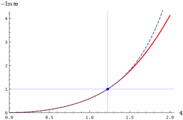
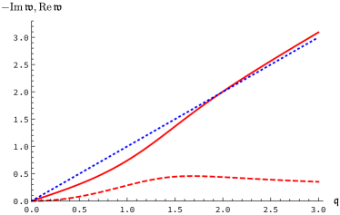
Figure 1: Dispersion relations of the hydrodynamic modes in the strongly coupled ${\cal N}=4$ SYM theory, obtained using the dual holographic description. The dispersion relations are plotted in terms of dimensionless $\mathfrak{w}\equiv\omega/2\pi T$ and $\mathfrak{q}\equiv|{\bf q}|/2\pi T$, with complex $\mathfrak{w}$ as functions of real positive $\mathfrak{q}$. The left panel shows $\mathfrak{w}_{\rm shear}(\mathfrak{q})$ for the shear mode, the right panel shows $\mathfrak{w}_{\rm sound}^{+}(\mathfrak{q})$ for one of the two sound modes. In the left panel, the actual $-{\rm Im}\,\mathfrak{w}_{\rm shear}(\mathfrak{q})$ for the shear mode is shown by the solid red curve, and the analytic hydrodynamic approximation to $O(\mathfrak{q}^{8})$ (computed in sec. 4.1) is shown by the dashed blue curve. The blue dot indicates the pole-skipping point at $\mathfrak{q}_{*}=\sqrt{3/2}$, $\mathfrak{w}_{*}=-i$, discussed in sec. 4.7. The right panel shows ${\rm Re}\,\mathfrak{w}_{\rm sound}^{+}(\mathfrak{q})$ (solid red curve) and $-{\rm Im}\,\mathfrak{w}_{\rm sound}^{+}(\mathfrak{q})$ (dashed red curve) for the “+” sound mode. The straight dotted line indicates the light cone $\mbox{Re}\,\mathfrak{w}=\mathfrak{q}$.

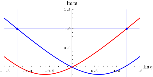
Figure 2: The analytically continued sound mode frequencies in the strongly coupled ${\cal N}=4$ SYM theory, obtained using the dual holographic description. The dimensionless frequencies $\mathfrak{w}_{\rm sound}^{\pm}$ of the two sound modes are plotted for purely imaginary dimensionless spatial momentum $\mathfrak{q}$, with the “+” branch in red and the “$-$” branch in blue. The frequencies $\mathfrak{w}_{\rm sound}^{\pm}$ are purely imaginary at imaginary $\mathfrak{q}$. At small momenta, the curves are linear with slopes $\pm v_{s}$, with $v_{s}=1/\sqrt{3}$. The curves pass through pole-skipping points $(\mathfrak{q}_{*},\mathfrak{w}_{*})=(\pm i\sqrt{3/2},i)$ indicated by the blue dots.

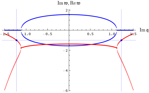
Figure 3: The first two (closest to the origin) poles of the retarded function of $T^{xy}$ in the strongly coupled ${\cal N}=4$ SYM theory, obtained using the dual holographic description. The locations of the poles are plotted as functions of the dimensionless wave vector for $\mathfrak{q}$ purely imaginary, with ${\rm Re}\,\mathfrak{w}$ shown in blue, and ${\rm Im}\,\mathfrak{w}$ shown in red. The dots indicate the points $(\mathfrak{q}_{*},\mathfrak{w}_{*})=(\pm i\sqrt{3/2},-i)$, where the response function of $T^{xy}$ exhibits pole-skipping.

A natural question to ask is whether pole-skipping happens within the domain of validity of the hydrodynamic approximation, as far as the convergence of the hydrodynamic derivative series is concerned. In other words, if the hydrodynamic dispersion relation $\mathfrak{w}_{i}(\mathfrak{q})$ has a finite radius of convergence $|\mathfrak{q}_{\rm c}^{i}|$ and pole-skipping in the corresponding response function happens at $|\mathfrak{q}_{*}^{i}|$, how does $|\mathfrak{q}_{\rm c}^{i}|$ compare with $|\mathfrak{q}_{*}^{i}|$? In the strongly coupled ${\cal N}=4$ SYM theory we have $|\mathfrak{q}_{\rm c}^{\rm sound}|=\sqrt{2}$, $|\mathfrak{q}_{\rm c}^{\rm shear}|\approx 1.49$ Grozdanov:2019kge , and $|\mathfrak{q}_{*}|=\sqrt{3/2}$. Thus $|\mathfrak{q}_{*}|<|\mathfrak{q}_{\rm c}|$, and therefore pole-skipping in correlation functions takes place within the convergence domain of the hydrodynamic derivative expansion. On the other hand, in the model of ref. Davison:2014lua , we have $|\mathfrak{q}_{\rm c}|=1/2$, $|\mathfrak{q}_{*}|=\sqrt{2}$, hence $|\mathfrak{q}_{*}|>|\mathfrak{q}_{\rm c}|$, so pole-skipping occurs outside the convergence domain of the hydrodynamic derivative expansion. This indicates that the “skipping” of hydrodynamic poles in retarded functions of energy and momentum densities is not directly related to the convergence radius of the derivative expansion in hydrodynamics.

More generally, pole-skipping singularities in real-time response functions at non-zero momentum do not have to have any relation to hydrodynamics at all. As an example, we consider response functions of spin-zero operators in 1+1 dimensional conformal field theory (CFT). For a primary operator, the Euclidean correlation function on ${\mathbb{R}}^{2}$ is fixed by conformal symmetry. Performing a conformal transformation to the cylinder ${\mathbb{R}}\times{\mathbb{S}}^{1}$ gives Euclidean thermal correlations functions DiFrancesco:1997nk , which can be Fourier transformed and analytically continued to produce exact real-time retarded functions $G^{R}(\mathfrak{w},\mathfrak{q})$ Son:2002sd . These functions have no hydrodynamic poles, yet we will see that there is an infinite number of pole-skippings at non-zero values of $(\mathfrak{q}_{*},\mathfrak{w}_{*})$. We discuss this in detail in section 5. Our conclusions and discussion of the issues raised in the paper appear in section 6.

2 Hydrodynamic dispersion relations as Puiseux series

2.1 Hydrodynamic spectral curves

We start with a brief review of how the hydrodynamic dispersion relations are derived. Consider hydrodynamics of a neutral homogeneous and isotropic relativistic fluid in flat space in $d_{s}$ spatial dimensions. We are interested in linearised fluctuations in a homogeneous and isotropic equilibrium state, $T^{\mu\nu}=T^{\mu\nu}_{\rm eq.}+\delta T^{\mu\nu}$, where $T^{\mu\nu}$ denotes the expectation value of the symmetric energy-momentum tensor operator, and the equilibrium state is characterised by $T^{00}_{\rm eq.}=\epsilon$, $T^{ij}_{\rm eq.}=p\delta^{ij}$, $T^{0i}_{\rm eq.}=0$, where $\epsilon$ and $p$ are the equilibrium energy density and pressure. The equations of hydrodynamics follow from the conservation of the energy-momentum tensor, $\partial_{\mu}T^{\mu\nu}=0$. Translation invariance of the equilibrium state implies that we can Fourier transform the fluctuations and take all variables to be proportional to $\exp{(-i\omega t+i{\bf q}{\cdot}{\bf x})}$. Furthermore, rotation invariance allows us to choose the direction of the $z$ axis along ${\bf q}$. We then have the following system of conservation equations for the linearised fluctuations:

$$-\omega\,\delta T^{0a}+q_{z}\,\delta T^{za} =0\,,$$ (8a)

$$-\omega\,\delta T^{00}+q_{z}\,\delta T^{z0} =0\,,$$ (8b)

$$-\omega\,\delta T^{0z}+q_{z}\,\delta T^{zz} =0\,,$$ (8c)

where we use the index $a$ and subsequent Latin indices to denote any of the $d_{s}-1$ spatial directions orthogonal to $z$.

The above conservation equations need to be supplemented by the constitutive relations which express $\delta T^{\mu\nu}$ in terms of the hydrodynamic degrees of freedom. For linearised hydrodynamics, a convenient choice of the degrees of freedom is the energy density $\delta T^{00}$ and momentum density $\delta T^{0i}$. This choice implies that we only need the constitutive relations for the spatial stress, $\delta T^{ij}=\delta T^{ij}(\delta T^{00},\delta T^{0k})$. The constitutive relations will contain derivatives of $\delta T^{00}$ and $\delta T^{0k}$, as is needed for example to describe the viscosity of fluids. We will organise the constitutive relations according to the number of derivatives of the hydrodynamic variables. The hydrodynamics of $k$-th order is determined by the constitutive relations in which $\delta T^{ij}$ contains up to $k$ derivatives of $\delta T^{00}$ and $\delta T^{0i}$. It is then straightforward to write down the linearised constitutive relations at any order, by noting that under the spatial $SO(d_{s})$, the stress fluctuation $\delta T^{ij}$ is a rank-two tensor, momentum density $\delta T^{0i}$ is a vector, and the energy density $\delta T^{00}$ is a scalar. For example, in the first-order hydrodynamics of ref. landau , we have

$$\delta T^{ij}\, =\delta^{ij}{\partial p\over\partial\epsilon}\,\delta T^{00}$$

$$-{1\over\epsilon+p}\left[\eta\left(\partial_{i}\,\delta T^{0j}+\partial_{j}\,\delta T^{0i}-{2\over d_{s}}\delta^{ij}\partial_{k}\delta T^{0k}\right)+\zeta\delta^{ij}\partial_{k}\,\delta T^{0k}\right]+\cdots\,,$$ (9)

where $\eta$ is the shear viscosity, $\zeta$ is the bulk viscosity, and the ellipses denote terms with more than one derivative of $\delta T^{00}$, $\delta T^{0i}$. Combining the constitutive relations (9) with the conservation equations (8) gives a system of linear equations for the fluctuations $\delta T^{00}$ and $\delta T^{0i}$. The equations have non-trivial solutions provided the corresponding determinant vanishes:

$$P_{1}({\bf q}^{2},\omega)\equiv\left(\omega+iD{\bf q}^{2}\right)^{d_{s}-1}\left(\omega^{2}+i\Gamma_{\!s}\omega{\bf q}^{2}-v_{s}^{2}{\bf q}^{2}\right)=0\,,$$ (10)

where $v_{s}^{2}=\partial p/\partial\epsilon$ is the speed of sound squared, and $D$, $\Gamma_{\!s}$ are defined by eqs. (3), (4).

In fact, rotation invariance implies that the most general linearised constitutive relations in momentum space take the following form:

$$\delta T^{nm}=\, -iA\left(q^{n}\delta T^{0m}+q^{m}\delta T^{0n}\right)+\delta T^{00}\left(Bq^{n}q^{m}+C\delta^{nm}\right)$$

$$\,+iq_{l}\delta T^{0l}\left(Dq^{n}q^{m}+E\delta^{nm}\right)\,,$$ (11)

where $A$, $B$, $C$, $D$, $E$ are scalar functions of $\omega$ and ${\bf q}^{2}$. Substituting the constitutive relations (11) into the conservation equations (8), we find a system of $d_{s}{+}1$ linear equations for $d_{s}{+}1$ hydrodynamic variables. This system has non-trivial solutions provided the determinant of the corresponding matrix vanishes. The vanishing of the determinant is equivalent to the vanishing of

$$P({\bf q}^{2},\omega)\equiv F_{\rm shear}^{d_{s}-1}F_{\rm sound}\,,$$ (12)

where

$$F_{\rm shear}({\bf q}^{2},\omega)\equiv\omega+i{\bf q}^{2}\gamma_{\eta}({\bf q}^{2},\omega)=0\,,$$ (13)

$$F_{\rm sound}({\bf q}^{2},\omega)\equiv\omega^{2}+i\omega{\bf q}^{2}\gamma_{s}({\bf q}^{2},\omega)-{\bf q}^{2}H({\bf q}^{2},\omega)=0\,.$$ (14)

Here the coefficients are $\gamma_{\eta}\equiv A$, $\gamma_{s}\equiv 2A-E-D{\bf q}^{2}$, $H=B{\bf q}^{2}+C$. Thus, the shear and the sound modes decouple as a consequence of rotation invariance.

If the constitutive relations (11) are given by a local derivative expansion, then the functions $\gamma_{\eta}({\bf q}^{2},\omega)$, $\gamma_{s}({\bf q}^{2},\omega)$ and $H({\bf q}^{2},\omega)$ are power series in $\omega$ and ${\bf q}^{2}$ with finite values at $\omega=0$, ${\bf q}^{2}=0$:

$$\gamma_{\eta}(0,0)=D\,,\qquad\gamma_{s}(0,0)=\Gamma_{\!s}\,,\qquad H(0,0)=v_{s}^{2}\,,$$ (15)

with $v_{s}$, $D$ and $\Gamma_{\!s}$ as above. Truncating the derivative expansion at order $k$ then gives a sequence of algebraic equations defined by finite polynomials in ${\bf q}^{2}$ and $\omega$,

$$F_{\rm shear}^{(k)}({\bf q}^{2},\omega)=0\,,$$ (16)

$$F_{\rm sound}^{(k)}({\bf q}^{2},\omega)=0\,.$$ (17)

For general complex $\omega$ and ${\bf q}^{2}$, eqs. (13), (14), or (16), (17) define complex algebraic curves^, which we will call hydrodynamic spectral curves. The complete dispersion relations of the $i$-th mode, $\omega_{i}=\omega_{i}({\bf q}^{2})$, can be obtained by solving eqs. (13), (14) for $\omega$, while the corresponding approximate expressions arising in $k$-th order hydrodynamics are found from eqs. (16), (17). The hydrodynamic dispersion relations are the solutions which satisfy $\omega_{i}({\bf q}^{2}\to 0)=0$. They correspond to infinite relaxation times for infinite-wavelength perturbations of conserved densities, i.e. to the conservation of energy and momentum.

Note that the polynomials $F_{\rm shear}^{(k)}({\bf q}^{2},\omega)$, $F_{\rm sound}^{(k)}({\bf q}^{2},\omega)$ are not defined uniquely because of the freedom to organise the derivative expansion in hydrodynamics, such as the choice of “frame” and the use of on-shell conditions Kovtun:2012rj ; Kovtun:2019hdm . As an example, the conservation equations (8) imply that the factors of $\omega$ in the constitutive relations (11) can be eliminated at each order in the derivative expansion. Thus one can organise the derivative expansion in such a way that the functions $\gamma_{\eta}({\bf q}^{2},\omega)$, $\gamma_{s}({\bf q}^{2},\omega)$ and $H({\bf q}^{2},\omega)$ are all $\omega$-independent at each given order in the expansion. Then eqs. (16), (17) give simple explicit expressions for $\omega_{\rm shear}({\bf q}^{2})$ and $\omega_{\rm sound}({\bf q}^{2})$ in terms of three scalar functions $\gamma_{\eta}({\bf q}^{2})$, $\gamma_{s}({\bf q}^{2})$ and $H({\bf q}^{2})$, whose small-${\bf q}$ limits are given by eq. (15). In this way of implementing the derivative expansion, the hydrodynamic dispersion relations are the only solutions to (16), (17). Of course, other choices of organising the derivative expansion are possible where the $\omega$-dependence in $\gamma_{\eta}({\bf q}^{2},\omega)$, $\gamma_{s}({\bf q}^{2},\omega)$ and $H({\bf q}^{2},\omega)$ is retained, and non-hydrodynamic (gapped) modes appear in addition to the hydrodynamic modes.

The above discussion was in the context of classical hydrodynamics. A similar factorisation of the shear and sound modes happens in the full response functions of the energy-momentum tensor, without any hydrodynamic assumptions Kovtun:2005ev . For example, for the wave vector along $z$, the shear mode is described by fluctuations of $\delta T^{0a}$, where the direction $a$ is orthogonal to $z$. The condition that the inverse of the equilibrium response function of the $T^{0a}$ operator vanishes can be written as $P_{\rm shear}({\bf q}^{2},\omega)=0$. In general, $P_{\rm shear}({\bf q}^{2},\omega)$ is a complicated function which describes both hydrodynamic (long-distance, long-time) and non-hydrodynamic (short-distance, short-time) physics. For small (appropriately defined) ${\bf q}^{2}$ and $\omega$, the exact $P_{\rm shear}({\bf q}^{2},\omega)$ will reduce to the above $F_{\rm shear}({\bf q}^{2},\omega)$, provided hydrodynamics is a valid effective description of the system. The same applies to the sound mode: the condition that the inverse of the equilibrium response function of the $T^{00}$ operator vanishes can be written as $P_{\rm sound}({\bf q}^{2},\omega)=0$. For small (relative to the appropriately defined scale) ${\bf q}^{2}$ and $\omega$, the exact $P_{\rm sound}({\bf q}^{2},\omega)$ will reduce to the above $F_{\rm sound}({\bf q}^{2},\omega)$, provided hydrodynamics is a valid effective description of the system. In this paper, we will only be studying physical systems in which the near-equilibrium physics governed by the conserved densities can be described by classical hydrodynamics. In other words, we will assume that the functions $\gamma_{\eta}({\bf q}^{2},\omega)$, $\gamma_{s}({\bf q}^{2},\omega)$, $H({\bf q}^{2},\omega)$ are defined by the exact response functions of the $T^{\mu\nu}$ operator.

2.2 Small-momentum expansions

For a given spectral curve, the small-${\bf q}^{2}$ expansion of the hydrodynamic dispersion relation $\omega_{i}({\bf q}^{2})$ can be found using the theorem of Puiseux (see Appendix A and refs. wall ; walker ; sendra ).

Starting with the shear mode, let us assume that $\gamma_{\eta}({\bf q}^{2},\omega)$ is analytic at $({\bf q}^{2},\omega)$=$(0,0)$ and thus eq. (13) defines an analytic curve for complex $({\bf q}^{2},\omega)\in\mathbb{C}^{2}$. This is of course not guaranteed a priori and should be established by independent methods, e.g. by finding the exact response function. The analyticity of $\gamma_{\eta}({\bf q}^{2},\omega)$ implies that $F_{\rm shear}({\bf q}^{2},\omega)$ is analytic at the origin as well, and, since $\partial F_{\rm shear}/\partial\omega=1\neq 0$ at $(0,0)$, the origin is a regular point of the analytic curve (13). Then the analytic implicit function theorem (see Appendix A) guarantees that for sufficiently small ${\bf q}^{2}$ and $\omega$, there exists a unique solution of eq. (13) of the form

$$\omega_{\rm shear}({\bf q}^{2})=-i\sum_{n=1}^{\infty}c_{n}{\bf q}^{2n}=-ic_{1}{\bf q}^{2}+O({\bf q}^{4})\,,$$ (18)

convergent in a neighbourhood of ${\bf q}^{2}=0$. The radius of convergence is determined by the location of the nearest to the origin critical point of the curve (13).

Continuing with the sound mode, let us again assume that $\gamma_{s}({\bf q}^{2},\omega)$ and $H({\bf q}^{2},\omega)$ are analytic functions at $(0,0)$. The function $F_{\rm sound}({\bf q}^{2},\omega)$ is then analytic at the origin as well. Now we have $\partial F_{\rm sound}/\partial\omega=0$ at $(0,0)$, and thus the origin is a critical point of the spectral curve. On the other hand, $\partial^{2}F_{\rm sound}/\partial\omega^{2}=2\neq 0$ at $(0,0)$, thus we expect the sound dispersion relation to have $p=2$ branches. The Puiseux series expansions are then given by eqs. (157), (158), in other words $\omega_{\rm sound}^{(j)}({\bf q}^{2})$ can be represented by series in non-negative powers of $({\bf q}^{2})^{1/m_{j}}$, where $m_{j}$ are positive integers, and $j=1,2$ labels the two branches corresponding to the two sound modes. Following the general analysis of algebraic curves, the integers $m_{j}$ may be found using the Newton’s polygon method (see refs. wall ; walker ; sendra for details). For analytic $\gamma_{s}$ and $H$, we have the expansions

$$\gamma_{s}({\bf q}^{2},\omega)=\sum\limits_{n,m=0}^{\infty}\gamma^{s}_{nm}\omega^{n}{\bf q}^{2m}\,,$$ (19)

$$H({\bf q}^{2},\omega)=\sum\limits_{n,m=0}^{\infty}H_{nm}\omega^{n}{\bf q}^{2m}\,.$$ (20)

The coefficients in front of various powers of $\omega$ in the expression (14) are then given by

$$\omega^{0}:\qquad-\sum\limits_{k=0}^{\infty}H_{0k}{\bf q}^{2k+2}\,,$$ (21)

$$\omega^{1}:\qquad i{\bf q}^{2}\gamma^{s}_{00}+\sum\limits_{k=1}^{\infty}\left(i\gamma^{s}_{0k}-H_{1k}\right){\bf q}^{2k+2}\,,$$ (22)

$$\omega^{2}:\qquad 1+\sum\limits_{k=0}^{\infty}\left(i\gamma^{s}_{1k}-H_{2k}\right){\bf q}^{2k+2}\,,$$ (23)

$$\omega^{3}:\qquad\sum\limits_{k=0}^{\infty}\left(i\gamma^{s}_{2k}-H_{3k}\right){\bf q}^{2k+2}\,,$$ (24)

$$\vdots\,$$ (25)

$$\omega^{n}:\qquad\sum\limits_{k=0}^{\infty}\left(i\gamma^{s}_{n-1k}-H_{nk}\right){\bf q}^{2k+2}\,.$$ (26)

The vertices of the Newton polygon are thus given by $(0,1+k_{0})$, $(1,1+k_{1})$, $(2,0)$, $(3,1+k_{3})$, $(4,1+k_{4})$, $\ldots$, where $k_{0},k_{1},\ldots$ are the smallest indices such that $H_{0k_{0}}\neq 0$ as well as $H_{0k_{1}}\neq 0$ or/and $\gamma^{s}_{0k_{1}}\neq 0$, etc. The Newton polygon for the sound mode is shown in fig. 4, where it is assumed that $H_{00}\neq 0$ and that either $H_{n,0}\neq 0$ or $\gamma^{s}_{n-1,0}\neq 0$ (or both) are non-zero for $n=3,4,\ldots$. The exponents of $x\equiv{\bf q}^{2}$ in the Puiseux series are given by the negative slopes of the polygon’s lines, i.e. by $1/2$ for $H_{00}\neq 0$. Thus $m_{j}=2$, and the lowest order term in the two branches is

$$\omega=\pm\sqrt{H_{00}}\,({\bf q}^{2})^{\frac{1}{2}}+\cdots\,.$$ (27)

From the Newton polygon, it is clear that $H_{00}\neq 0$ is the necessary and sufficient condition for the fractional powers of ${\bf q}^{2}$ to appear in the dispersion relation. In the hydrodynamic derivative expansion, $H_{00}=\partial p/\partial\epsilon=v_{s}^{2}$ is the speed of sound squared. One may have $H_{00}=0$ at the point of a phase transition (see e.g. ref. Parnachev:2005hh ) in which case the dispersion relation contains only positive powers of ${\bf q}^{2}$.

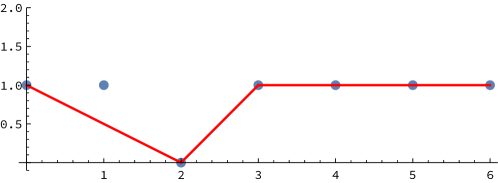
Figure 4: The Newton polygon for the sound mode.

Generically, for $H_{00}=v_{s}^{2}\neq 0$, the sound mode dispersion relation will be given by the two branches of Puiseux series in $({\bf q}^{2})^{1/2}$ converging in some neighbourhood of the point ${\bf q}^{2}=0$,

$$\omega_{\rm sound}^{\pm}({\bf q}^{2})=-i\sum_{n=1}^{\infty}a_{n}e^{\pm\frac{i\pi n}{2}}({\bf q}^{2})^{\frac{n}{2}}=\pm a_{1}({\bf q}^{2})^{\frac{1}{2}}+ia_{2}{\bf q}^{2}\mp a_{3}({\bf q}^{2})^{\frac{3}{2}}+O({\bf q}^{4})\,,$$ (28)

where $a_{n}\in\mathbb{R}$ and $a_{1}=c_{s}$ is the speed of sound. In particular, for ${\bf q}^{2}=e^{\pm i\pi}|{\bf q}^{2}|$, the functions $\omega_{\rm sound}^{\pm}({\bf q}^{2})$ are purely imaginary as anticipated in ref. Grozdanov:2017ajz .

2.3 Convergence of the hydrodynamic series

The shear and sound dispersion relation series (18) and (28) have non-zero radii of convergence as long as the corresponding spectral curves (13) and (14) are given by the functions of ${\bf q}^{2}$ and $\omega$ analytic at the origin $(0,0)$. One way to find the radius of convergence of the series is to analyse the behaviour of the coefficients $a_{n}$, $c_{n}$ at large $n$. This behaviour will of course depend on the microscopic details of the particular physical system, and may be difficult to study in practice (see, however, ref. Withers:2018srf ). Instead, here we use the spectral curves to determine the radii of convergence.

The Puiseux analysis implies that the domain of convergence of Puiseux series centred e.g. at the origin is the circle whose radius is set by the distance from the origin to the nearest critical point of the associated spectral curve. Critical points of the spectral curve $F({\bf q}^{2},\omega)=0$, where ${\bf q}^{2},\omega\in\mathbb{C}$, are determined by the conditions

$$F({\bf q}^{2}_{\rm c},\omega_{\rm c})=0\,,\qquad\frac{\partial F}{\partial\omega}({\bf q}^{2}_{\rm c},\omega_{\rm c})=0\,.$$ (29)

There are $p>1$ branches of the solution $\omega=\omega({\bf q}^{2})$ in the vicinity of the critical point, provided that

$$F({\bf q}^{2}_{\rm c},\omega_{\rm c})=0\,,\qquad\frac{\partial F}{\partial\omega}({\bf q}^{2}_{\rm c},\omega_{\rm c})=0\,,\,\ldots,\,\frac{\partial^{p}F}{\partial\omega^{p}}({\bf q}^{2}_{\rm c},\omega_{\rm c})\neq 0\,.$$ (30)

For example, the origin $(0,0)$ is the critical point (with $p=2$) of the sound hydrodynamic spectral curve (14), as discussed in section 2.2. If the spectral curves happen to be known exactly or approximately (as will be the case in the holographic models we study below), eqs. (29) provide an efficient method to find the radii of convergence, without performing the large-$n$ analysis of the expansion coefficients.

When the function $F({\bf q}^{2},\omega)$ is a polynomial, the condition (29) means that the equation $F({\bf q}^{2},\omega)=0$, where $F({\bf q}^{2},\omega)$ is considered as a polynomial in $\omega$ with ${\bf q}^{2}$-dependent coefficients, has multiple roots at $\omega=\omega_{\rm c}$. This is equivalent to the condition that the discriminant of the polynomial $F({\bf q}^{2},\omega)$ vanishes. As an example, consider the first-order hydrodynamics of landau , where the spectral curves following from eq. (10) are

$$F_{\rm shear}^{(1)}({\bf q}^{2},\omega)=\omega+iD{\bf q}^{2}=0\,,$$ (31)

$$F_{\rm sound}^{(1)}({\bf q}^{2},\omega)=\omega^{2}+i\Gamma_{\!s}\omega{\bf q}^{2}-v_{s}^{2}{\bf q}^{2}=0\,.$$ (32)

These equations are simple enough to be solved explicitly: eq. (31) is solved by $\omega=-iD{\bf q}^{2}$, whereas the solutions of eq. (32) are

$$\omega^{\pm}_{\rm sound}({\bf q}^{2})=-\frac{i\Gamma_{\!s}}{2}\,{\bf q}^{2}\pm\sqrt{v_{s}^{2}{\bf q}^{2}\left(1-\frac{\Gamma_{\!s}^{2}{\bf q}^{2}}{4v_{s}^{2}}\right)}=\pm v_{s}q-\frac{i\Gamma_{\!s}}{2}\,q^{2}+\cdots\,,$$ (33)

where in the expansion we only kept terms quadratic in $q\equiv\sqrt{{\bf q}^{2}}$, since we expect the coefficients in front of the higher powers of $q$ to be modified by higher-derivative terms in the hydrodynamic expansion. The series in $q$ on the right-hand side of eq. (33) has the radius of convergence

$$R^{(1)}_{\rm sound}=\frac{2v_{s}}{\Gamma_{\!s}}\,,$$ (34)

determined by the branch points of the square root in eq. (33) or, equivalently, by the zeros of the discriminant $(-\Gamma_{\!s}^{2}{\bf q}^{4}+4v_{s}^{2}{\bf q}^{2})$ of the polynomial (32). Since first-order hydrodynamics can only be trusted for $|q|\ll 2v_{s}/\Gamma_{\!s}=R^{(1)}_{\rm sound}$, the result (34) is only an approximation. Alternatively, applying the condition (29) to the spectral curve (32), we find

$${\bf q}^{2}_{\rm c}=\frac{4v_{s}^{2}}{\Gamma_{\!s}^{2}}\,,\qquad\omega_{\rm c}^{\rm(sound)}=-i\frac{2v_{s}}{\Gamma_{\!s}}\,,$$ (35)

which coincides with (34). In what follows, we will be studying models where the convergence radii of the small-${\bf q}$ expansions can be determined from the exact response functions of the theory, without resorting to the derivative expansion of hydrodynamics.

3 A holographic model with translation symmetry breaking

To illustrate the methods discussed in section 2.3, we consider the holographic model with translation symmetry breaking Andrade:2013gsa , studied, in particular, in ref. Davison:2014lua . The model is a bottom-up gravity construction in $4d$ describing a hypothetical dual $2+1$-dimensional QFT with broken translational invariance. In the context of the present paper, the significance of the construction discussed in ref. Davison:2014lua lies in the fact that it provides exact analytic formulae for the current and energy-momentum correlator two-point functions at a special, self-dual symmetry point (see section 4 of ref. Davison:2014lua for details). In particular, among the poles of the correlation function, one finds a gapless excitation whose dispersion relation is known analytically, possibly a unique example in holography.

The bulk action of the model is given by Andrade:2013gsa ; Davison:2014lua (see also ref. Blake:2018leo )

$$S=\int\,d^{4}x\sqrt{-g}\left(R-2\Lambda-\frac{1}{2}\sum_{i=1}^{2}\partial^{\mu}\phi_{i}\partial_{\mu}\phi_{i}-\frac{1}{4}F_{\mu\nu}F^{\mu\nu}\right),$$ (36)

where $\Lambda=-3/L^{2}$ (we set $L=1$ in the following). The background solution of interest involves the AdS-Schwarzschild black brane with translational invariance broken by the linear dilaton fields, and a vanishing Maxwell field.

First, we recast the setup of ref. Davison:2014lua in the form more convenient for our purposes, having in mind the variables used in ref. Kovtun:2005ev . The metric at the special symmetry point has the form (see section 4 of ref. Davison:2014lua )

$$ds^{2}=-\frac{r_{0}^{2}}{u}f(u)\,dt^{2}+\frac{r_{0}^{2}}{u}\left(dx^{2}+dy^{2}\right)+\frac{du^{2}}{4fu^{2}}\,,$$ (37)

where $f=1-u$, and we have used the coordinate $u=r_{0}^{2}/r^{2}$. The horizon is located at $u=1$ and the boundary at $u=0$. The Hawking temperature of the background is $T=r_{0}/2\pi$. The dilaton fields are given by $\phi_{1}=\sqrt{2}r_{0}x$ and $\phi_{2}=\sqrt{2}r_{0}y$. They will not play any role in the following.

Considering the Maxwell field fluctuations in the background (37), coupled to the current operator on the boundary, one finds the equations of motion

$$a_{t}^{\prime\prime}+\frac{1}{2u}a_{t}^{\prime}-\frac{1}{4uf}\left(\mathfrak{q}^{2}a_{t}+\mathfrak{w}\mathfrak{q}\,a_{x}\right) =0\,,$$ (38)

$$a_{x}^{\prime\prime}+\frac{1-3u}{2uf}a_{x}^{\prime}+\frac{1}{4uf^{2}}\left(\mathfrak{q}\mathfrak{w}a_{t}+\mathfrak{w}^{2}a_{x}\right) =0\,,$$ (39)

$$\mathfrak{w}a_{t}^{\prime}+\mathfrak{q}fa_{x}^{\prime} =0\,,$$ (40)

where $\mathfrak{w}=\omega/2\pi T=\omega/r_{0}$, $\mathfrak{q}=k/2\pi T=k/r_{0}$, and the momentum $k$ is directed along $x$. For the gauge-invariant variable (the longitudinal component of the electric field) $E_{x}=\mathfrak{q}a_{t}+\mathfrak{w}a_{x}$ Kovtun:2005ev , the equation of motion reads

$$E_{x}^{\prime\prime}+\frac{\mathfrak{w}^{2}(1-3u)-\mathfrak{q}^{2}f^{2}}{2uf(\mathfrak{w}^{2}-\mathfrak{q}^{2}f)}\,E_{x}^{\prime}+\frac{\mathfrak{w}^{2}-\mathfrak{q}^{2}f}{4uf^{2}}\,E_{x}=0\,.$$ (41)

The equation (41) has 4 regular singular points (located at $u=0,1,1-\mathfrak{w}^{2}/\mathfrak{q}^{2},\infty)$ and thus is of the Heun type. The indices of this equation are, respectively,

$$\,u =0: 0,1/2\,$$ (42)

$$\,u =1: \pm i\mathfrak{w}/2\,$$ (43)

$$\,u =1-\frac{\mathfrak{w}^{2}}{\mathfrak{q}^{2}}: 0,2\,$$ (44)

$$\,u =\infty: \frac{1}{4}\left(1\pm\sqrt{1-4\mathfrak{q}^{2}}\right)\,.$$ (45)

Note that the local solution at $u=0$ does not contain logarithms. The exact solution to eq. (41) can be written as

$$E_{x}(u)=\frac{4uf}{\mathfrak{q}}G^{\prime}(u)+\frac{2f}{\mathfrak{q}}G(u)\,,$$ (46)

where $G\equiv a_{t}^{\prime}$ is the solution of the hypergeometric equation

$$G^{\prime\prime}-\frac{5u-3}{2uf}G^{\prime}+\frac{\mathfrak{w}^{2}-\mathfrak{q}^{2}f-2f}{4uf^{2}}\,G=0\,,$$ (47)

obeying the incoming wave boundary condition at $u=1$:

$$G=\frac{\mathfrak{q}}{2i\mathfrak{w}}x^{-i\mathfrak{w}/2}\,_{2}F_{1}\left(\frac{3-2i\mathfrak{w}-\sqrt{1-4\mathfrak{q}^{2}}}{4},\frac{3-2i\mathfrak{w}+\sqrt{1-4\mathfrak{q}^{2}}}{4};1-i\mathfrak{w};x\right)\,,$$ (48)

where $x=1-u$ and the normalisation is chosen to ensure $E_{x}\rightarrow(1-u)^{-i\mathfrak{w}/2}\left(1+\cdots\right)$ at $u\rightarrow 1$.

3.1 The exact spectral curve

For the boundary value of the electric field, we find

$$E_{x}(u=0;\mathfrak{q}^{2},\mathfrak{w})\equiv F(\mathfrak{q}^{2},\mathfrak{w})=\frac{2\sqrt{\pi}\ \Gamma(-i\mathfrak{w})}{\Gamma\left[A_{+}(\mathfrak{q}^{2},\mathfrak{w})\right]\Gamma\left[A_{-}(\mathfrak{q}^{2},\mathfrak{w})\right]}\,,$$ (49)

where

$$A_{\pm}=\frac{1}{4}\left(1\pm\sqrt{1-4\mathfrak{q}^{2}}-2i\mathfrak{w}\right)\,.$$ (50)

The condition $E_{x}(u=0)=0$ determines the quasinormal modes and thus the poles of the corresponding current-current correlators Son:2002sd ; Kovtun:2005ev . One can also write down the explicit analytic expressions for the correlators themselves Davison:2014lua , but this will not be necessary: the expression $F(\mathfrak{q}^{2},\mathfrak{w})=0$, where $F(\mathfrak{q}^{2},\mathfrak{w})$ is given by eq. (49), is the exact spectral curve containing all information about the poles of the two-point function. There are two sequences of quasinormal frequencies

$$\mathfrak{w}_{n}^{\pm}(\mathfrak{q}^{2})=-i\left(2n_{\pm}+\frac{1}{2}\right)\pm\frac{i}{2}\sqrt{1-4\mathfrak{q}^{2}}\,,\qquad n_{\pm}=0,1,2\ldots\,.$$ (51)

The solutions $E_{x,n_{\pm}}^{\pm}(u)$ themselves (the quasinormal modes) have the form

$$E^{\pm}_{x,n_{\pm}}(u)=\sqrt{u}\,\left(1-u\right)^{-n_{\pm}-\frac{1}{4}\pm\frac{1}{4}\sqrt{1-4\mathfrak{q}^{2}}}\,P^{\pm}_{n_{\pm}}(u,\mathfrak{q}^{2})\,,$$ (52)

where $P^{\pm}_{n_{\pm}}(u,\mathfrak{q}^{2})$ are polynomials of degree $n_{\pm}$ in $u$ with $\mathfrak{q}^{2}-$dependent coefficients. In particular,

$$E^{\pm}_{x,0}(u)=\sqrt{u}\,\left(1-u\right)^{-\frac{1}{4}\pm\frac{1}{4}\sqrt{1-4\mathfrak{q}^{2}}}\,.$$ (53)

Note that apart from the prefactors determined by the indices, the solutions (52) are polynomials, with $P_{0}^{\pm}=1$. We are especially interested in the gapless mode

$$\mathfrak{w}=\mathfrak{w}_{0}^{+}\, =-\frac{i}{2}\left(1-\sqrt{1-4\mathfrak{q}^{2}}\right)=\frac{i}{2}\sum_{n=1}^{\infty}(-1)^{n}{1/2\choose n}\left(4\mathfrak{q}^{2}\right)^{n}$$

$$=-i\mathfrak{q}^{2}-i\mathfrak{q}^{4}-2i\mathfrak{q}^{6}-5i\mathfrak{q}^{8}-14i\mathfrak{q}^{10}+\cdots\,.$$ (54)

The power series in the second line of eq. (54) converges in the circle $|\mathfrak{q}^{2}|<1/4$, due to the branch point singularity of the function at $\mathfrak{q}^{2}=1/4$ evident from eq. (54). The same conclusion can be obtained by analysing critical points of the spectral curve (49). Indeed, the critical points are determined by the equations (29) whose solutions are $\mathfrak{w}_{n_{+}}^{+}(\mathfrak{q}^{2})=\mathfrak{w}_{n_{-}}^{-}(\mathfrak{q}^{2})$, i.e.

$$\mathfrak{q}^{2}_{\rm c}=\frac{1}{4}-\left(n_{+}-n_{-}\right)^{2},$$ (55a)

$$\mathfrak{w}_{\rm c}=-\frac{i}{2}\left[1+2\left(n_{+}+n_{-}\right)\right].$$ (55b)

It is also clear that $\partial^{2}_{\mathfrak{w}}F(\mathfrak{q}^{2}_{\rm c},\mathfrak{w}_{\rm c})\neq 0$ and thus there are two branches of the spectral curve emerging at each critical point. Put simply, the critical points occur when the two quasinormal frequencies in eq. (51) collide. This happens for real $\mathfrak{q}$ in case of $n_{+}=n_{-}$, and for purely imaginary $\mathfrak{q}$ for $n_{+}\neq n_{-}$. The critical point closest to the origin $\mathfrak{q}^{2}=0$ is at $\mathfrak{q}^{2}=1/4$ (it corresponds to the collision of the modes $\mathfrak{w}_{0}^{+}$ and $\mathfrak{w}_{0}^{-}$). This value determines the radius of convergence of the series in eq. (54).

Exact spectral curves are rare: in addition to (49), we are aware of only one example (involving the exact R-current two-point correlators in ${\cal N}=4$ SYM theory in appropriate limit Myers:2007we ) for a QFT in dimension higher than $1+1$, and even in that case it is only known exactly for $\mathfrak{q}^{2}=0$:

$$F_{R}(\mathfrak{q}^{2}=0,\mathfrak{w})=2^{-\frac{(1+i)\mathfrak{w}}{2}}\,\frac{\Gamma\left[1-i\mathfrak{w}\right]}{\Gamma\left[1-\frac{(1+i)\mathfrak{w}}{2}\right]\Gamma\left[1+\frac{(1-i)\mathfrak{w}}{2}\right]}\,.$$ (56)

One can use the Weierstrass decomposition

$$\frac{1}{\Gamma(z)}=ze^{\gamma z}\prod_{n=1}^{\infty}\left(1+\frac{z}{n}\right)e^{-\frac{z}{n}}\,,$$ (57)

where $\gamma$ is the Euler–Mascheroni constant, to write eqs. (49), (56) as infinite products: this ilustrates explicitly why the critical points determined by the condition (29) correspond to multiple roots of (infinite order) polynomials.

3.2 The hydrodynamic approximation to the spectral curve

The expansion of the expression $\mathfrak{w}F(\mathfrak{q}^{2},\mathfrak{w})$ for small $\mathfrak{w}$, $\mathfrak{q}$ (assuming the scaling $\mathfrak{w}\rightarrow\epsilon\mathfrak{w}$, $\mathfrak{q}^{2}\rightarrow\epsilon\mathfrak{q}^{2}$ with $\epsilon\to 0$) truncated at order $\mathfrak{w}^{k}$, $\mathfrak{q}^{2k}$ is a polynomial $F_{k}(\mathfrak{q}^{2},\mathfrak{w})$, with

$$F_{1}(\mathfrak{q}^{2},\mathfrak{w})=\mathfrak{w}+i\mathfrak{q}^{2}\,,$$ (58)

$$F_{2}(\mathfrak{q}^{2},\mathfrak{w})=\mathfrak{w}+i\mathfrak{q}^{2}-i\left[\mathfrak{w}^{2}\ln{2}-\mathfrak{q}^{4}\left(1-\ln{2}\right)\right]\,,$$ (59)

$$F_{3}(\mathfrak{q}^{2},\mathfrak{w})=\mathfrak{w}+i\mathfrak{q}^{2}-i\left[\mathfrak{w}^{2}\ln{2}-\mathfrak{q}^{4}\left(1-\ln{2}\right)\right]$$

$$-\frac{i}{12}\left[\mathfrak{q}^{6}\left(\pi^{2}-6(\ln{2}-2)^{2}\right)-6i\mathfrak{q}^{4}\mathfrak{w}\ln^{2}2-6i\mathfrak{w}^{3}\ln^{2}2+\mathfrak{q}^{2}\mathfrak{w}^{2}(\pi^{2}-6\ln^{2}2)\right]\,,$$ (60)

and so on. Using this expansion to solve the equation $\mathfrak{w}F(\mathfrak{q}^{2},\mathfrak{w})=0$ for $\mathfrak{w}$ perturbatively in $\mathfrak{q}^{2}$, one reproduces the series in eq. (54). The equation $F_{k}(\mathfrak{q}^{2},\mathfrak{w})=0$ defines the hydrodynamic spectral curve of order $k$ as discussed in section 2. At each order, the critical points are determined by the condition (29). In fig. 5, we plot the corresponding value $|\mathfrak{q}_{\rm c}^{2}|$ for each of the spectral curves $F_{k}(\mathfrak{q}^{2},\mathfrak{w})=0$ for $k=2,3,\ldots,13$. The resulting points converge rapidly to the exact value $|\mathfrak{q}_{\rm c}^{2}|=1/4$.

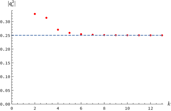
Figure 5: The approximations to the exact position of the critical point $|\mathfrak{q}_{\rm c}^{2}|=1/4$ in the holographic model with broken translation symmetry determined from the hydrodynamic algebraic curves $F_{k}(\mathfrak{q}^{2},\mathfrak{w})=0$ as a function of $k$.

3.3 Pole-skipping in the full response functions

Finally, we comment on the relationship between the critical point defining the hydrodynamic series radius of convergence and the pole-skipping point in the holographic model with broken translation symmetry, which occurs at $|\mathfrak{q}_{*}^{2}|=2>|\mathfrak{q}_{\rm c}^{2}|$ Blake:2018leo . Because gapless excitations in the current and the energy density correlators have the same dispersion relation, we can directly use $\mathfrak{w}(\mathfrak{q})$ from eq. (54) to discuss both the charge and the energy sectors. At the pole-skipping point, the hydrodynamic series stated in the second line of eq. (54) diverges but can be resummed using the Borel transform

$$\mathcal{B}\mathfrak{w}(\mathfrak{q}) =\frac{i}{2}\sum_{n=1}^{\infty}\frac{(-1)^{n}}{n!}{1/2\choose n}\left(4\mathfrak{q}^{2}\right)^{n}$$ (61)

$$=-\frac{i}{2}\left[1-e^{2\mathfrak{q}^{2}}\left((1-4\mathfrak{q}^{2})I_{0}(2\mathfrak{q}^{2})+4\mathfrak{q}^{2}I_{1}(2\mathfrak{q}^{2})\right)\right]\,,$$ (62)

where $I_{n}(x)$ is the modified Bessel function. Since this is a series in $\mathfrak{q}^{2}$ and not $\mathfrak{q}$, the corresponding Borel integral has the form

$$\mathbf{\Omega}(\mathfrak{q})=\int_{0}^{\infty}dt\,e^{-t}\mathcal{B}\mathfrak{w}(\mathfrak{q}\sqrt{t})=\mathcal{I}_{1}+\mathcal{I}_{2}+\mathcal{I}_{3}+\mathcal{I}_{4}\,,$$ (63)

where

$$\mathcal{I}_{1} =-\frac{i}{2}\int_{0}^{\infty}dt\,e^{-t}=-\frac{i}{2}\,,$$ (64)

$$\mathcal{I}_{2} =\frac{i}{2}\int_{0}^{\infty}dt\,e^{-t}e^{2\mathfrak{q}^{2}t}I_{0}(2\mathfrak{q}^{2}t)=\frac{i}{2}\frac{1}{\sqrt{1-4\mathfrak{q}^{2}}}\,,$$ (65)

$$\mathcal{I}_{3} =-i\int_{0}^{\infty}dt\,e^{-t}(2\mathfrak{q}^{2}t)e^{2\mathfrak{q}^{2}t}I_{0}(2\mathfrak{q}^{2}t)=-2i\mathfrak{q}^{2}\frac{(1-2\mathfrak{q}^{2})}{(1-4\mathfrak{q}^{2})^{3/2}}\,,$$ (66)

$$\mathcal{I}_{4} =i\int_{0}^{\infty}dt\,e^{-t}(2\mathfrak{q}^{2}t)e^{2\mathfrak{q}^{2}t}I_{1}(2\mathfrak{q}^{2}t)=4i\frac{\mathfrak{q}^{2}\sqrt{\mathfrak{q}^{4}}}{(1-4\mathfrak{q}^{2})^{3/2}}\,,$$ (67)

each with their respective region of $\mathfrak{q}$ for which the integral converges. Together, we find that the Borel integral representation (63) of the series converges for $\mathfrak{q}\in\mathbb{C}$ in the region defined by the function $\mathcal{C}(\mathfrak{q})$:

$$\mathcal{C}(\mathfrak{q})\equiv\text{Re}[\mathfrak{q}^{2}]<1/4\,.$$ (68)

This is a significant improvement over the convergence region of the hydrodynamic power series, $|\mathfrak{q}^{2}|<|\mathfrak{q}_{\rm c}^{2}|=1/4$. In particular, the Borel series is well suited for studying purely imaginary $\mathfrak{q}$. By writing $\mathfrak{q}=i\ell$, with $\ell\in\mathbb{R}$, we see that

$$\mathcal{C}(i\ell)=\text{Re}[-\ell^{2}]=-\text{Re}[\ell^{2}]\leq 0<1/4\,.$$ (69)

Hence, the Borel representation of the series converges for all values of imaginary $\mathfrak{q}$, including $\mathfrak{w}(\mathfrak{q})$ at the chaos point $\mathfrak{w}_{*}(\mathfrak{q}_{*}=\sqrt{2}i)=i$. Finally, for $\mathfrak{q}$ such that $\mathcal{C}(\mathfrak{q})<1/4$, it is easy to check that the sum of four terms in (63) indeed reproduces the full dispersion relation (54).

4 Response functions in strongly coupled ${\cal N}=4$ SYM theory

In this section, we use holographic duality to find the spectral curves, determine the radii of convergence of hydrodynamic series and analyse the pole-skipping phenomenon in the three channels of the response function of the energy-momentum tensor in the ${\cal N}=4$ $SU(N_{c})$ SYM theory at infinite ’t Hooft coupling and infinite $N_{c}$. The details of the duality are well known, and the necessary ingredients can be found e.g. in refs. Son:2007vk ; Policastro:2002se ; Kovtun:2005ev . In short, holography reduces the study of the response functions to the analysis of the fluctuations of the dual gravitational background involving a black hole with translationally invariant horizon—the AdS-Schwarzschild black brane.

The equations of motion describing fluctuations of the gravitational background dual to finite-temperature ${\cal N}=4$ SYM theory are of the Heun type Starinets:2002br , and the exact analytic solution for the spectral curve similar to eq. (49) is not available. The equations can be solved perturbatively and analytically in $\mathfrak{w}\ll 1$, $\mathfrak{q}\ll 1$, as was done in refs. Policastro:2002se ; Policastro:2002tn , thereby giving a hydrodynamic approximation to the spectral curve, or numerically, for arbitrary $\mathfrak{w}$ and $\mathfrak{q}$, along the lines of ref. Kovtun:2005ev . In this section, we consider and compare these two approaches.

4.1 Shear mode: hydrodynamic approximation to the spectral curve

We start with the analysis of the shear channel of the energy-momentum tensor response function Kovtun:2005ev . In the hydrodynamic approximation, the spectral curve can be found analytically from the boundary value of the solution to the ODE obeyed by one of the components of the shear perturbation in dual gravity (see section 6.2 of ref. Policastro:2002se for details):

$$G^{\prime\prime}(u)-\left(\frac{2u}{f}-\frac{i\mathfrak{w}}{1-u}\right)\,G^{\prime}(u)+\frac{1}{f}\left(2+\frac{i\mathfrak{w}}{2}-\frac{\mathfrak{q}^{2}}{u}+\frac{\mathfrak{w}^{2}[4-u(1+u)^{2}]}{4uf}\right)G(u)=0\,,$$ (70)

where $G$ is regular at $u=1$. Rescaling $\mathfrak{w}\rightarrow\lambda^{2}\mathfrak{w}$ and $\mathfrak{q}^{2}\rightarrow\lambda^{2}\mathfrak{q}^{2}$, assuming $\lambda\ll 1$, and looking for a perturbative solution of the form

$$G(u)=\sum_{n=0}^{\infty}\lambda^{2n}G_{n}(u)\,,$$ (71)

we find the following equation for coupled components $G_{n}$, $G_{n-1}$, $G_{n-2}$:

$$G_{n}^{\prime\prime} -\frac{2u}{f}G_{n}^{\prime}+\frac{2}{f}G_{n}$$

$$+\frac{i\mathfrak{w}}{1-u}G_{n-1}^{\prime}+\frac{i\mathfrak{w}}{2f}G_{n-1}-\frac{\mathfrak{q}^{2}}{uf}G_{n-1}$$

$$+\frac{\mathfrak{w}^{2}[4-u(1+u)^{2}]}{4uf^{2}}G_{n-2}=0\,,$$ (72)

where $G_{n}=0$ for $n<0$, and we can set $G_{0}(1)=1$, $G_{i}(1)=0$, $i\geq 1$, without loss of generality. The explicit formulae for $G_{0}(u)$, $G_{1}(u)$ and $G_{2}(u)$ obeying the boundary conditions at $u=1$ are written in Appendix B. The solution of the homogeneous equation

$$g^{\prime\prime}-\frac{2u}{f}\,g^{\prime}+\frac{2}{f}\,g=0$$ (73)

is given by $g=C_{1}\,g_{1}(u)+C_{2}\,g_{2}(u)$, where

$$g_{1} =u\,,$$ (74)

$$g_{2} =\frac{u}{2}\ln{\frac{1+u}{1-u}}-1\,.$$ (75)

Note that the Wronskian is $W(g_{1},g_{2})=1/f$. Then one can write the following expression for $G_{n}$, $n\geq 2$:

$$G_{n}(u) =g_{1}(u)\int_{u}^{1}g_{2}(t)f(t){\cal F}_{n}(t)dt-g_{2}(u)\int_{u}^{1}g_{1}(t)f(t){\cal F}_{n}(t)dt$$

$$+C_{1}\,g_{1}(u)+C_{2}\,g_{2}(u)\,,$$ (76)

where

$${\cal F}_{n}(u)=-\frac{i\mathfrak{w}}{1-u}G_{n-1}^{\prime}-\frac{i\mathfrak{w}}{2f}G_{n-1}+\frac{\mathfrak{q}^{2}}{uf}G_{n-1}-\frac{\mathfrak{w}^{2}[4-u(1+u)^{2}]}{4uf^{2}}G_{n-2}\,.$$ (77)

Boundary conditions at $u=1$ (regularity of $G_{n}(u)$ at $u=1$ and $G_{n}(1)=0$ for $n>0$) require $C_{1}=0$, $C_{2}=0$. Thus, we have the equation determining $G_{n}$ from $G_{n-1}$ and $G_{n-2}$,

$$G_{n}(u) =u\int_{u}^{1}(1-t^{2})\left(\frac{t}{2}\ln{\frac{1+t}{1-t}}-1\right){\cal F}_{n}(t)dt$$

$$-\left(\frac{u}{2}\ln{\frac{1+u}{1-u}}-1\right)\int_{u}^{1}t(1-t^{2}){\cal F}_{n}(t)dt\,,$$ (78)

where ${\cal F}_{n}$ is given by eq. (77). This can be written as

$$G_{n}(u) =\frac{u}{2}\int_{u}^{1}t(1-t^{2})\ln{\left[\frac{1+t-u-ut}{1-t+u-ut}\right]}{\cal F}_{n}(t)\,dt$$

$$+\int_{u}^{1}(t-u)(1-t^{2}){\cal F}_{n}(t)dt\,,$$ (79)

or

$$G_{n}(u)=\, \int_{u}^{1}\left\{\frac{ut}{2}\ln{\left[\frac{1+t-u-ut}{1-t+u-ut}\right]}+t-u\right\}(1-t^{2})\,{\cal F}_{n}(t)\,dt\,.$$ (80)

Note that ${\cal F}_{n}(t)\sim 1/(1-t)$ at $t\rightarrow 1$, and so all integrals converge. In particular,

$$G_{n}(0)=\int_{0}^{1}t(1-t^{2}){\cal F}_{n}(t)dt\,.$$ (81)

The explicit expressions for $G_{i}(0)$, with $i=1,2,3,4$, are written in Appendix B. The results for $G_{0}(0)$, $G_{1}(0)$ and $G_{2}(0)$ coincide with those in ref. Baier:2007ix . The results for $G_{3}(0)$ and $G_{4}(0)$ are new. The condition $G(0)=0$ at this order in the hydrodynamic expansion defines the algebraic curve

$$F(\mathfrak{q}^{2},\mathfrak{w})=-i\mathfrak{w}+\frac{\mathfrak{q}^{2}}{2}$$

$$+\frac{\mathfrak{q}^{4}}{4}-\frac{i\mathfrak{w}\mathfrak{q}^{2}\ln{2}}{4}+\frac{\mathfrak{w}^{2}\ln{2}}{2}$$

$$+i\mathfrak{w}^{3}\left(\frac{\pi^{2}}{24}+\ln{2}-\frac{3}{8}\ln^{2}2\right)+\mathfrak{q}^{6}\left(\frac{\ln{2}}{4}-\frac{1}{8}\right)+i\mathfrak{w}\mathfrak{q}^{4}\left(\frac{1}{4}-\frac{\ln 2}{8}\right)$$

$$+\mathfrak{q}^{2}\mathfrak{w}^{2}\left(\frac{\pi^{2}}{48}-\frac{\ln{2}}{2}-\frac{\ln^{2}2}{16}\right)+\mathfrak{q}^{8}\left(-\frac{1}{16}+\frac{\pi^{2}}{64}-\frac{\ln{2}}{8}\right)-\mathfrak{q}^{4}\mathfrak{w}^{2}\left(\frac{\pi^{2}}{96}+\left(12-7\ln{2}\right)\frac{\ln{8}}{96}\right)$$

$$-i\mathfrak{q}^{6}\mathfrak{w}\left(\frac{\pi^{2}}{96}+\left(-5+\ln{4}\right)\frac{\ln{64}}{96}\right)+\mathfrak{w}^{4}\left(\left(24-5\ln{2}\right)\frac{\ln^{2}{2}}{48}+\frac{\pi^{2}}{48}\left(-4+\ln{8}\right)-\frac{1}{2}\zeta(3)\right)$$

$$+i\mathfrak{q}^{2}\mathfrak{w}^{3}\left(-\frac{\pi^{2}\ln{2}}{96}+\left(-24+\ln{2}\right)\frac{\ln^{2}{2}}{96}+\frac{3}{16}\zeta(3)\right)=0\,.$$ (82)

Here, $\zeta(z)$ is the Riemann zeta function. Solving eq. (82) perturbatively in $\mathfrak{q}^{2}$, one finds the dispersion relation for the shear mode

$$\mathfrak{w}\, =-\frac{i}{2}\,\mathfrak{q}^{2}-\frac{i(1-\ln{2})}{4}\,\mathfrak{q}^{4}-\frac{i(24\ln^{2}2-\pi^{2})}{96}\,\mathfrak{q}^{6}$$

$$-\frac{i(2\pi^{2}(5\ln{2}-1)-21\zeta(3)-24\ln{2}[1+\ln{2}(5\ln{2}-3)])}{384}\mathfrak{q}^{8}\,+O(\mathfrak{q}^{10})\,.$$ (83)

The first two terms in (83) agree with the ones obtained in refs. Policastro:2002se and Baier:2007ix , respectively.

Encouraged by the success of finding the critical point in the holographic model with broken translation symmetry in section 3, we can apply the condition (29) to the polynomial (82). Truncating (82) at linear (in $\mathfrak{w}$ and $\mathfrak{q}^{2}$), quadratic, cubic and quartic order, correspondingly, we obtain the algebraic curves $F_{k}(\mathfrak{q}^{2},\mathfrak{w})=0$ for $k=1,2,3,4$. Using the condition (29), we find that there are no solutions at $k=1$, whereas for $k=2,3,4$, we have

$$k=2: \mathfrak{q}_{\rm c}^{2} \approx-1.380398\pm 0.865925i\,, \mathfrak{w}_{\rm c} \approx\pm 0.216481+1.097596i\,,$$ (84)

$$k=3: \mathfrak{q}_{\rm c}^{2} \approx 0.164953\pm 1.151910i\,, \mathfrak{w}_{\rm c} \approx\pm 0.735771+0.164407i\,,$$ (85)

$$k=4: \mathfrak{q}_{\rm c}^{2} \approx 0.548173\pm 0.988705i\,, \mathfrak{w}_{\rm c} \approx\pm 0.706672-0.140043i\,.$$ (86)

In fig. 6, the $k=2,3,4$ approximations are shown in the complex plane of $\mathfrak{q}_{\rm c}^{2}$ together with the “exact” value $\mathfrak{q}_{\rm c}^{2}\approx 1.8906469\pm 1.1711505i$ obtained via the quasinormal level-crossing method (see section 4.2). In contrast with the holographic model with broken translation symmetry (see fig. 5), the convergence is slow (admittedly, we only have 3 points in the present case). However, we learn an important lesson, namely, that the critical point can be located at a generic complex value of $\mathfrak{q}^{2}$. In the next section, we use a more efficient method of the quasinormal modes level-crossing to determine the critical points.

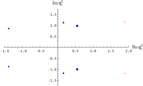
Figure 6: Approximations to the position of the critical point in the complex $\mathfrak{q}_{\rm c}^{2}$ plane in the shear channel of the ${\cal N}=4$ SYM theory arising from the order $k$ hydrodynamic polynomials $F_{k}(\mathfrak{q}^{2},\mathfrak{w})=0$ (circles for $k=2$, triangles for $k=3$, squares for $k=4$). The “exact” position $\mathfrak{q}_{\rm c}^{2}\approx 1.8906469\pm 1.1711505i$ (see section 4.2) is marked by red asterisks.

4.2 Shear mode: full spectral curve

To compute the spectral curve numerically for all values of $\mathfrak{q}^{2}$ and $\mathfrak{w}$, it is more convenient to use the ODE obeyed by the gauge-invariant perturbations. The gauge-invariant shear mode gravitational perturbations of the AdS-Schwarzschild black brane are described by the function $Z_{1}(u)$, where $u$ is the radial coordinate ranging from $u=0$ (asymptotic boundary) to $u=1$ (event horizon) Kovtun:2005ev . The function $Z_{1}(u)$ obeys the equation

$$Z_{1}^{\prime\prime}-\frac{(\mathfrak{w}^{2}-\mathfrak{q}^{2}f)f-u\mathfrak{w}^{2}f^{\prime}}{uf(\mathfrak{w}^{2}-\mathfrak{q}^{2}f)}Z_{1}^{\prime}+\frac{\mathfrak{w}^{2}-\mathfrak{q}^{2}f}{uf^{2}}Z_{1}=0\,,$$ (87)

where $f(u)=1-u^{2}$, and the solution must obey the incoming wave boundary condition at the horizon, $Z_{1}(u)\sim(1-u)^{-i\mathfrak{w}/2}$ as $u\to 1$ Son:2002sd ; Kovtun:2005ev . The full shear spectral curve is then given by

$$F(\mathfrak{q}^{2},\mathfrak{w})=Z_{1}(u=0;\mathfrak{q}^{2},\mathfrak{w})=0\,.$$ (88)

The spectral curve (88) can be determined numerically by e.g. using $N$ terms of the Frobenius series solution at $u=1$ Kovtun:2005ev .

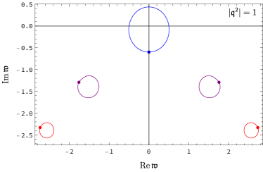
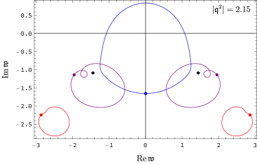
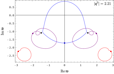
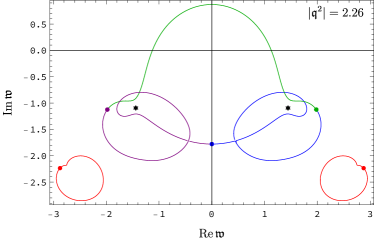
Figure 7: Quasinormal spectrum (poles of the retarded energy-momentum tensor two-point function in the ${\cal N}=4$ SYM theory) in the shear channel plotted in the complex $\mathfrak{w}$-plane for different values of the complex momentum $\mathfrak{q}^{2}=|\mathfrak{q}^{2}|e^{i\theta}$. Large dots in all four plots correspond to the location of the poles for purely real momentum, $\mathfrak{q}^{2}$ (i.e. at $\theta=0$) Kovtun:2005ev . The hydrodynamic shear pole is the blue pole closest to the real axis in the top left panel. As $\theta$ increases from $0$ to $2\pi$, each pole moves in a counter-clockwise direction, following the trajectory of its colour. At $|\mathfrak{q}^{2}|=1$, all poles follow a closed orbit (top left panel). At $|\mathfrak{q}^{2}|=2.15$ (top right panel), the trajectory of the hydrodynamic pole intersects the trajectories of the two nearest gapped poles. With $|\mathfrak{q}^{2}|$ further increasing to $|\mathfrak{q}^{2}|=2.21$, the poles nearly collide at the positions marked by asterisks (bottom left panel). The actual collision occurs at the critical point with the momentum (89), $|\mathfrak{q}_{\rm c}^{2}|\approx 2.224$. At $|\mathfrak{q}^{2}|=2.26$ (bottom right panel), the orbits of the three poles closest to the origin $(\mathfrak{w}=0)$ are no longer closed: the hydrodynamic pole and the two gapped poles exchange their positions cyclically as the phase $\theta$ increases from $0$ to $2\pi$. This is a manifestation of the quasinormal mode level-crossing. The dispersion relation $\mathfrak{w}(\mathfrak{q}^{2})$ therefore has branch point singularities in the complex momentum squared plane at $\mathfrak{q}_{\rm c}^{2}$.

The stability of the numerical procedure is ensured by checking that adding several more terms to the series does not appreciably change the result. Applying (numerically) the criterion (29) to (88), we find the critical point closest to the origin,

$$\mathfrak{q}_{\rm c}^{2} \approx 1.8906469\pm 1.1711505i\,, \mathfrak{w}_{\rm c} \approx\pm 1.4436414-1.0692250i\,,$$ (89)

implying the convergence radius of the shear mode dispersion relation $|\mathfrak{q}_{\rm shear}^{\rm c}|\approx 1.49131$. There are other critical points with $|\mathfrak{q}^{2}|>|\mathfrak{q}_{\rm shear}^{\rm c}|$. The first three of them are located at

$$\mathfrak{q}_{\rm c,1}^{2} \approx-2.37737\,, \mathfrak{w}_{\rm c,1} \approx-1.64659i\,,$$ (90)

$$\mathfrak{q}_{\rm c,2}^{2} \approx-3.11051\pm 0.8105i\,, \mathfrak{w}_{\rm c,2} \approx\pm 1.41043-2.87086i\,,$$ (91)

$$\mathfrak{q}_{\rm c,3}^{2} \approx 2.90692\pm 1.66606i\,, \mathfrak{w}_{\rm c,3} \approx\pm 2.38819-2.13154i\,.$$ (92)

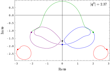
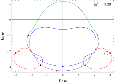
Figure 8: Quasinormal spectrum (poles of the retarded energy-momentum tensor two-point function in the ${\cal N}=4$ SYM theory) in the shear channel plotted in the complex $\mathfrak{w}$-plane for different values of the complex momentum $\mathfrak{q}^{2}=|\mathfrak{q}^{2}|e^{i\theta}$. Large dots in all four plots correspond to the location of the poles for purely real momentum, $\mathfrak{q}^{2}$ (i.e. at $\theta=0$) Kovtun:2005ev . The second critical point (occuring at $|\mathfrak{q}_{\rm c,1}^{2}|\approx 2.377$) is marked by asterisks in the figures showing the trajectories just before and just after the pole collision (top panels). With $|\mathfrak{q}^{2}|$ further increasing, the second pair of gapped modes becomes involved in the collisions leading to the third critical point at $|\mathfrak{q}_{\rm c,2}^{2}|\approx 3.214$ (bottom panels).

In figs. 7 and 8, we show the corresponding quasinormal spectrum (solutions $\mathfrak{w}=\mathfrak{w}(\mathfrak{q}^{2})$ of eq. (88)) in the complex plane of frequency $\mathfrak{w}$, parametrised by $\mathfrak{q}^{2}$. The difference with previous works is that now, we treat $\mathfrak{q}^{2}$ as a generic complex variable, $\mathfrak{q}^{2}=|\mathfrak{q}^{2}|e^{i\theta}$, and vary its phase, $\theta\in[0,2\pi]$, at specific fixed values of the magnitude $|\mathfrak{q}^{2}|$. From eq. (87), it is clear that if $Z_{1}(u;\mathfrak{q},\mathfrak{w})$ is a solution satisfying the incoming wave boundary condition at the horizon, then $Z_{1}(u;\mathfrak{q},-\mathfrak{w})$ is also a solution. The spectrum in figs. 7 and 8 therefore appears to be symmetric with respect to the imaginary axis. For real $\mathfrak{q}^{2}$, the spectrum coincides with the one originally found in ref. Nunez:2003eq .

At small $|\mathfrak{q}^{2}|$, the poles follow closed orbits as the phase $\theta$ varies from $0$ to $2\pi$ (fig. 7, top panels). With the parameter $|\mathfrak{q}^{2}|$ increasing, the poles start feeling the presence of each other, and their orbits become more complicated. Finally, at $|\mathfrak{q}_{\rm c}^{2}|\approx 2.224$, the hydrodynamic shear pole collides with one of the two closest non-hydrodynamic poles (see fig. 7, bottom panels). For $|\mathfrak{q}^{2}|>|\mathfrak{q}_{\rm c}^{2}|$, those three poles no longer have closed orbits: as the phase $\theta$ varies from $0$ to $2\pi$, they interchange their positions cyclically (fig. 7, bottom right panel). For even larger $|\mathfrak{q}^{2}|$, other gapped poles become involved in this collective motion of quasinormal modes in a similar manner (fig. 8).

The phenomenon observed in figs. 7, 8 is the quasinormal spectrum level-crossing, reminiscent of the well-known effect in quantum mechanics. Indeed, for real $\mathfrak{q}^{2}$, the real and imaginary parts of the quasinormal frequencies do not exhibit level-crossing (see e.g. figs. 13 and 14 in ref.  Nunez:2003eq ). For complex momentum $\mathfrak{q}^{2}=|\mathfrak{q}^{2}|e^{i\theta}$, the real and imaginary parts of the shear hydrodynamic mode and the nearest gapped mode do cross at the fixed phase $\theta\approx 0.338858\pi$ and $|\mathfrak{q}^{2}|=|\mathfrak{q}_{\rm c}^{2}|\approx 2.224$, as shown in fig. 9. A similar effect at a purely imaginary momentum was observed by Withers (see fig. 3 in ref. Withers:2018srf ), and numerous instances of pole collisions (i.e. quasinormal level-crossings) at real momenta were reported earlier (see e.g. Davison:2011ek ; Davison:2014lua ; Grozdanov:2016vgg ; Grozdanov:2016fkt ; Grozdanov:2018ewh ; Baggioli:2018nnp ; Baggioli:2018vfc ; Grozdanov:2018fic ; Grozdanov:2018gfx ; Gushterov:2018spg ; Davison:2018ofp ; Baggioli:2019jcm ).

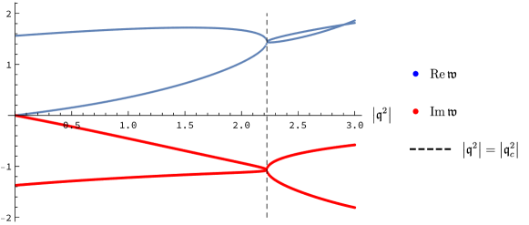
Figure 9: Quasinormal spectrum level-crossing: the real (blue curves) and the imaginary (red curves) parts of the hydrodynamic shear mode and the closest gapped quasinormal mode dispersion relations plotted as functions of $|\mathfrak{q}^{2}|$ at the fixed phase $\theta\approx 0.338858\pi$ of the complex momentum $\mathfrak{q}^{2}=|\mathfrak{q}^{2}|e^{i\theta}$. At $|\mathfrak{q}^{2}|=|\mathfrak{q}_{\rm c}^{2}|\approx 2.224$, the level-crossing occurs.

4.3 Sound mode: hydrodynamic approximation to the spectral curve

The gauge-invariant perturbation corresponding to the sound mode obeys the equation Kovtun:2005ev

$$Z_{2}^{\prime\prime}-\frac{3\mathfrak{w}^{2}(1+u^{2})+\mathfrak{q}^{2}(2u^{2}-3u^{4}-3)}{uf(3\mathfrak{w}^{2}+\mathfrak{q}^{2}(u^{2}-3))}\,Z_{2}^{\prime}$$

$$+\frac{3\mathfrak{w}^{4}+\mathfrak{q}^{4}(3-4u^{2}+u^{4})+\mathfrak{q}^{2}(4u^{5}-4u^{3}+4u^{2}\mathfrak{w}^{2}-6\mathfrak{w}^{2})}{uf^{2}(3\mathfrak{w}^{2}+\mathfrak{q}^{2}(u^{2}-3))}\,Z_{2}=0\,.$$ (93)

The full sound spectral curve is constructed from the solution $Z_{2}(u;\mathfrak{q}^{2},\mathfrak{w})$ obeying the incoming wave boundary conditions at the horizon and is given by

$$F(\mathfrak{q}^{2},\mathfrak{w})=Z_{2}(u=0;\mathfrak{q}^{2},\mathfrak{w})=0\,.$$ (94)

Similarly to the shear mode case, one can first find a hydrodynamic approximation to eq. (94) analytically. For $\mathfrak{w}\ll 1$ and $\mathfrak{q}\ll 1$, eq. (93) can be solved perturbatively. Writing

$$Z_{2}(u)=\left(1-u^{2}\right)^{-\frac{i\mathfrak{w}}{2}}\sum_{n=0}^{\infty}\lambda^{n}z_{n}(u)$$ (95)

to enforce the boundary condition at the horizon, rescaling $\mathfrak{w}\to\lambda\mathfrak{w}$ and $\mathfrak{q}\to\lambda\mathfrak{q}$, and assuming $\lambda\ll 1$, we find the following recurrence relation for the functions $z_{n}(u)$:

$$z_{n}^{\prime\prime}- \frac{3\left(1+u^{2}\right)\mathfrak{w}^{2}-\left(3-2u^{2}+3u^{4}\right)\mathfrak{q}^{2}}{u\left(1-u^{2}\right)\left[3\mathfrak{w}^{2}-\left(3-u^{2}\right)\mathfrak{q}^{2}\right]}z_{n}^{\prime}-\frac{4u^{2}\mathfrak{q}^{2}}{\left(1-u^{2}\right)\left[3\mathfrak{w}^{2}-\left(3-u^{2}\right)\mathfrak{q}^{2}\right]}z_{n}$$

$$+\frac{2iu\mathfrak{w}}{1-u^{2}}z_{n-1}^{\prime}-\frac{4iu^{2}\mathfrak{w}\mathfrak{q}^{2}}{\left(1-u^{2}\right)\left[3\mathfrak{w}^{2}-\left(3-u^{2}\right)\mathfrak{q}^{2}\right]}z_{n-1}$$

$$+\frac{\left(1+u+u^{2}\right)\mathfrak{w}^{2}-\left(1+u\right)\mathfrak{q}^{2}}{u\left(1-u\right)\left(1+u\right)^{2}}z_{n-2}=0\,,$$ (96)

with $z_{-1}=z_{-2}=0$. To fourth order in $\lambda$, we find the hydrodynamic algebraic curve to be (see also eq. (4.18) in ref. Baier:2007ix )

$$F(\mathfrak{q}^{2},\mathfrak{w}) =\frac{\mathfrak{q}^{2}}{2}-\frac{3\mathfrak{w}^{2}}{2}-i\mathfrak{w}\mathfrak{q}^{2}+\frac{\mathfrak{w}^{4}}{16}\left(\pi^{2}-12\ln^{2}2+24\ln{2}\right)-\frac{\mathfrak{q}^{4}}{12}\left(2\ln{2}-8\right)$$

$$-\frac{\mathfrak{w}^{2}\mathfrak{q}^{2}}{48}\left(\pi^{2}-12\ln^{2}2+48\ln 2\right)=0\,.$$ (97)

The form of $F(\mathfrak{q}^{2},\mathfrak{w})$ for general $\mathfrak{w}$ and $\mathfrak{q}$ is at present not known to $O(\lambda^{5})$. However, assuming that $\mathfrak{w}$ can be expanded in a series in powers of $\mathfrak{q}$, in ref. Grozdanov:2015kqa , $F(\mathfrak{q}^{2})$ was computed to order $O(\lambda^{5})=O(\mathfrak{q}^{5})$, which was sufficient to find the coefficient in the sound mode dispersion relation multiplying $\mathfrak{q}^{4}$ (i.e. to third order in the gradient expansion):

$$\mathfrak{w}\, =\pm\frac{1}{\sqrt{3}}\mathfrak{q}-\frac{i}{3}\mathfrak{q}^{2}\pm\frac{3-2\ln 2}{6\sqrt{3}}\mathfrak{q}^{3}-\frac{i\left(\pi^{2}-24+24\ln 2-12\ln^{2}2\right)}{108}\mathfrak{q}^{4}\,+O(\mathfrak{q}^{5})\,.$$ (98)

The first two terms in the dispersion relation (98) coincide with those obtained in ref. Policastro:2002tn . The third term was found in ref. Baier:2007ix (see also ref. Bhattacharyya:2008jc ). The fourth term was computed in ref. Grozdanov:2015kqa . It appeared earlier in ref. Bu:2014ena (with an incorrect coefficient in front of $\ln{2}$) and (correctly) in ref. Bu:2015bwa in the context of the fluid-gravity correspondence.

Here, we use the form of the algebraic curve (97) and apply the condition (29) to show that in the sound channel, the small $\mathfrak{w}$ and $\mathfrak{q}$ expansion of the spectral curve $F(\mathfrak{q}^{2},\mathfrak{w})$ qualitatively correctly accounts for two sets of critical points:

$$\mathfrak{q}_{\rm c}^{2} =0\,, \mathfrak{w}_{\rm c} =0\,,$$ (99)

$$\mathfrak{q}_{\rm c}^{2} \approx 0.34739\pm 0.56763i\,, \mathfrak{w}_{\rm c} \approx\pm 0.71165+0.39882i\,.$$ (100)

The critical point (99) is expected from hydrodynamics, as discussed in section 2.2. Having in mind the results of section 4.1, we may expect that the hydrodynamic approximation (100) to the position of the non-trivial critical point is not accurate. In section 4.4 we confirm this by finding the critical point exactly.

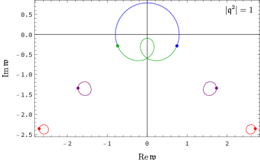
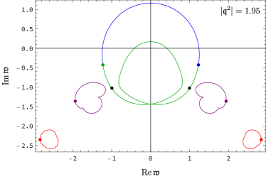
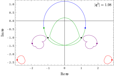
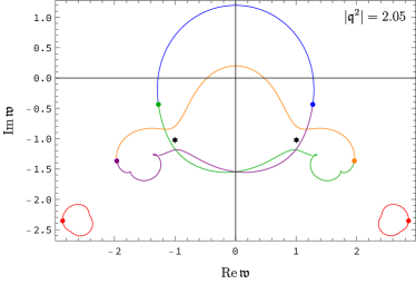
Figure 10: Quasinormal spectrum (poles of the retarded energy-momentum tensor two-point function in the ${\cal N}=4$ SYM theory) in the sound channel plotted in the complex $\mathfrak{w}$-plane for different values of the complex momentum $\mathfrak{q}^{2}=|\mathfrak{q}^{2}|e^{i\theta}$. Large dots in all four plots correspond to the location of the poles for purely real momentum, $\mathfrak{q}^{2}$ (i.e. at $\theta=0$) Kovtun:2005ev . The hydrodynamic sound poles are the blue and the green poles closest to the real axis. As $\theta$ is tuned from $0$ to $2\pi$, each pole moves in a counter-clockwise direction and follows the trajectory of its colour. At $|\mathfrak{q}^{2}|=1$ (top left panel), all poles follow a closed orbit. At $|\mathfrak{q}^{2}|=1.95$ (top right panel), the trajectory of the two hydrodynamic sound poles comes close to the trajectories of the nearest gapped poles. With $|\mathfrak{q}^{2}|$ further increasing to $|\mathfrak{q}^{2}|=1.98$, the poles nearly collide at the positions marked by asterisks (bottom left panel). The actual collision occurs at the critical value of the momentum (101), $|\mathfrak{q}_{\rm c}^{2}|=2$. At $|\mathfrak{q}^{2}|=2.05$ (bottom right panel), the orbits of the four uppermost poles are no longer closed: the hydrodynamic poles and the two gapped poles exchange their positions cyclically as the phase $\theta$ increases from $0$ to $2\pi$—again, a manifestation of the quasinormal mode level-crossing. The dispersion relation $\mathfrak{w}(\mathfrak{q})$ therefore has branch cuts starting at $\mathfrak{q}_{\rm c}$.

4.4 Sound mode: full spectral curve

As discussed in section 4.3, the origin (99) is a critical point of the sound mode dispersion relation $\mathfrak{w}=\mathfrak{w}(\mathfrak{q}^{2})$, as predicted by hydrodynamics (see section 2.2). Proceeding as in section 4.2, we find the first set of critical points nearest to the origin at

$$\mathfrak{q}_{\rm c}^{2} =\pm 2i\,, \mathfrak{w}_{\rm c} =\pm 1-i\,,$$ (101)

within the limits of our numerical accuracy. Curiously, although eq. (93) looks rather complicated, one can check that with $\mathfrak{w}$ and $\mathfrak{q}^{2}$ given by (101), a simple analytic solution satisfying the correct boundary conditions at $u=1$ and $u=0$ is available. Explicitly, the two solutions corresponding to the pair of critical points in (101) are

$$(\mathfrak{q}_{\rm c}^{2}=2i,\mathfrak{w}_{\rm c}=1-i): Z_{2}(u) =\mathcal{C}^{+}_{2}\left(1-u\right)^{-\frac{i\left(1-i\right)}{2}}\left(1+u\right)^{-\frac{1-i}{2}}u^{2}\left(u-3i\right)\,,$$ (102)

$$(\mathfrak{q}_{\rm c}^{2}=-2i,\mathfrak{w}_{\rm c}=-1-i): Z_{2}(u) =\mathcal{C}^{-}_{2}\left(1-u\right)^{-\frac{i\left(-1-i\right)}{2}}\left(1+u\right)^{\frac{-1-i}{2}}u^{2}\left(u+3i\right)\,,$$ (103)

where $\mathcal{C}_{2}^{\pm}$ are arbitrary constants. Although we were not able to show analytically that $\partial_{\mathfrak{w}}Z(u=0)=0$ at (101) as well, we have verified this numerically to high precision. The existence of the critical point (101) implies that the convergence radius of the sound mode dispersion relation is given by $|\mathfrak{q}_{\rm sound}^{\rm c}|=\sqrt{2}\approx 1.41421$. The next set of critical points is located at

$$\mathfrak{q}_{\rm c}^{2} \approx-0.01681\pm 3.12967i\,, \mathfrak{w}_{\rm c} \approx\pm 1.90134-2.04492i\,.$$ (104)

The behaviour of poles in the complex frequency plane is shown in figs. 10 and 11, and the quasinormal level-crossing phenomenon is presented in fig. 12.

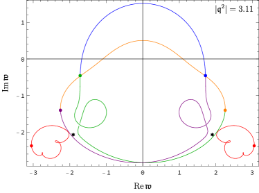
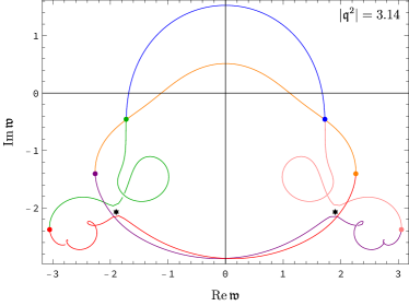
Figure 11: Quasinormal spectrum (poles of the retarded energy-momentum tensor two-point function in the ${\cal N}=4$ SYM theory) in the sound channel plotted in the complex $\mathfrak{w}$-plane for different values of the complex momentum $\mathfrak{q}^{2}=|\mathfrak{q}^{2}|e^{i\theta}$. Large dots in all four plots correspond to the location of the poles for purely real momentum, $\mathfrak{q}^{2}$ (i.e. at $\theta=0$) Kovtun:2005ev . What is shown is the level-crossing phenomenon for the critical points in eq. (104).

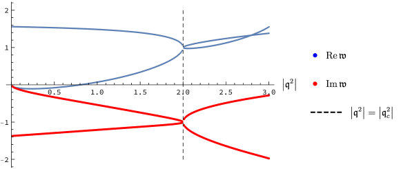
Figure 12: Quasinormal spectrum level-crossing in the sound channel: the real (blue curves) and the imaginary (red curves) parts of the hydrodynamic sound mode and the closest gapped quasinormal mode dispersion relations plotted as functions of $|\mathfrak{q}^{2}|$ at the fixed phase $\theta=\pi/2$ of the complex momentum $\mathfrak{q}^{2}=|\mathfrak{q}^{2}|e^{i\theta}$. At $|\mathfrak{q}^{2}|=|\mathfrak{q}_{\rm c}^{2}|=2$, the level-crossing occurs.

4.5 Scalar mode: full spectral curve

In the scalar channel, the gauge-invariant metric perturbation $Z_{3}(u)$ obeys the equation Kovtun:2005ev

$$Z_{3}^{\prime\prime}-\frac{(1+u^{2})}{uf}\,Z_{3}^{\prime}+\frac{\mathfrak{w}^{2}-\mathfrak{q}^{2}f}{uf^{2}}\,Z_{3}=0\,.$$ (105)

The full spectral curve is constructed from the solution $Z_{3}(u;\mathfrak{q}^{2},\mathfrak{w})$ obeying the incoming wave boundary conditions at the horizon and is given by

$$F(\mathfrak{q}^{2},\mathfrak{w})=Z_{3}(u=0;\mathfrak{q}^{2},\mathfrak{w})=0\,.$$ (106)

The quasinormal spectrum in the scalar channel has no hydrodynamic modes, but it exhibits the phenomenon of level-crossing for the gapped modes, as shown in fig. 13. The first two sets of critical points nearest to the origin are given by

$$\mathfrak{q}_{\rm c}^{2} \approx-1.25309\,, \mathfrak{w}_{\rm c} \approx-1.76937i\,,$$ (107a)

$$\mathfrak{q}_{\rm c}^{2} \approx-1.49704\pm 0.36674i\,, \mathfrak{w}_{\rm c} \approx\mp 1.47977-2.79404i\,.$$ (107b)

These are branch points in the scalar (gapped) dispersion relation $\mathfrak{w}=\mathfrak{w}(\mathfrak{q}^{2})$.

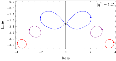
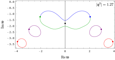
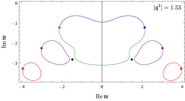
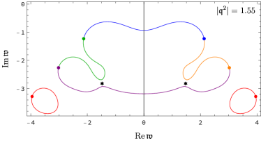
Figure 13: Quasinormal spectrum (poles of the retarded energy-momentum tensor two-point function in the ${\cal N}=4$ SYM theory) in the scalar channel plotted in the complex $\mathfrak{w}$-plane for different values of the complex momentum $\mathfrak{q}^{2}=|\mathfrak{q}^{2}|e^{i\theta}$. Large dots in all plots correspond to the location of the poles for purely real momentum, $\mathfrak{q}^{2}$ (i.e. at $\theta=0$) Kovtun:2005ev . There are no hydrodynamic modes in this channel, but the gapped modes exhibit the level-crossing phenomena at complex values of momenta given by eq. (107).

4.6 Analytic structure of the hydrodynamic dispersion relations

From the discussion above, it is clear that the shear mode dispersion relation $\mathfrak{w}_{\rm shear}(\mathfrak{q}^{2})$ is an analytic function of complex $\mathfrak{q}^{2}$ in the circle $|\mathfrak{q}^{2}|<|\mathfrak{q}_{\rm c}^{2}|\approx 2.224$. Since the appropriate second derivative of the spectral curve at the critical point is non-zero (i.e. $p=2$ in the Puiseux language of section 2.3; see eq. (30)) which corresponds to a collision of two quasinormal modes, the critical point is the branch point singularity of the square root type, with the Puiseux series in powers of $\pm\sqrt{\mathfrak{q}^{2}-\mathfrak{q}_{\rm c}^{2}}$ providing the extension beyond the radius of convergence. We show the critical points, the radius of convergence and the appropriate branch cuts in the complex plane of $\mathfrak{q}^{2}$ in fig. 14 (left panel).

For the sound mode dispersion relation, considered as a function of $\mathfrak{q}^{2}\in\mathbb{C}$, the origin is a branch point, and the corresponding Puiseux series is given by eq. (28). It will be more convenient to consider the sound dispersion relation $\mathfrak{w}_{\rm sound}(\mathfrak{q})$ as a function of complexified magnitude $\mathfrak{q}\in\mathbb{C}$ of the wave-vector ${\bf q}$. The critical points, the radius of convergence and the appropriate branch cuts in the complex plane of $\mathfrak{q}$ are shown in fig. 14 (right panel).

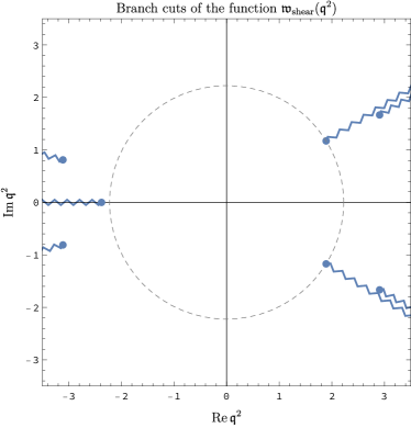
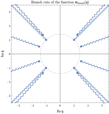
Figure 14: Branch point singularities, branch cuts and the domain of hydrodynamic series convergence for the shear mode in the complex $\mathfrak{q}^{2}$-plane (left panel) and the sound mode in the complex $\mathfrak{q}$-plane (right panel).

4.7 Pole-skipping in the full response functions

As already discussed in the Introduction, analytically continued hydrodynamic modes appear to be connected to the parameters of an OTOC related to the microscopic many-body quantum chaos. The apparent connection is provided by the phenomenon of pole-skipping Grozdanov:2017ajz ; Blake:2017ris ; Blake:2018leo ; Grozdanov:2018kkt , whereby a pole and a zero of a two-point correlation function collide for some $\mathfrak{w},\mathfrak{q}\in\mathbb{C}$. In the sound channel of the energy-momentum tensor retarded two-point function, the pole-skipping has been studied in the context of holography Grozdanov:2017ajz ; Blake:2018leo ; Grozdanov:2018kkt , effective field theory Blake:2017ris and two-dimensional conformal field theory in the limit of large central charge Haehl:2018izb . Here, we extend the discussion in refs. Grozdanov:2017ajz ; Blake:2018leo ; Grozdanov:2018kkt to show that pole-skipping also occurs in other channels.

Consider a retarded two-point function $G^{R}(\mathfrak{w},\mathfrak{q})$ of the energy-momentum tensor components at finite temperature. Schematically, and modulo tensor structure, the correlator can be written as

$$G^{R}(\mathfrak{w},\mathfrak{q})\sim\frac{b(\mathfrak{w},\mathfrak{q})}{a(\mathfrak{w},\mathfrak{q})}\,,$$ (108)

where $a(\mathfrak{w},\mathfrak{q})$ necessarily contains a gapless hydrodynamic mode $\mathfrak{w}=\mathfrak{w}(\mathfrak{q})$ (either shear or sound) in the appropriate channels Kovtun:2005ev . More generally, let ${\cal Z}_{d}=\{\mathfrak{w}=\mathfrak{w}(\mathfrak{q}):a(\mathfrak{w}(\mathfrak{q}),\mathfrak{q})=0\}$ and ${\cal Z}_{n}=\{\mathfrak{w}=\mathfrak{w}(\mathfrak{q}):b(\mathfrak{w}(\mathfrak{q}),\mathfrak{q})=0\}$, where we assume for simplicity that all zeros are simple. Then, pole-skipping occurs at generically complex $(\mathfrak{q}_{*},\mathfrak{w}_{*})\in\mathcal{P}={\cal Z}_{n}\cap{\cal Z}_{d}$.

For theories with available gravity dual descriptions, the set $\mathcal{P}$ can be determined directly either by computing ${\cal Z}_{n}$ and ${\cal Z}_{d}$ (the set ${\cal Z}_{d}$ is nothing but the quasinormal spectrum) or from the dual gravity equations of motion (see below). In the case of energy-momentum tensor correlators of the ${\cal N}=4$ SYM theory in the limit of infinite $N_{c}$ and infinite ‘t Hooft coupling $\lambda$, pole-skipping in the three channels occurs at points $(\mathfrak{q}_{*},\mathfrak{w}_{*})$ given by

$${\rm Sound\,channel}: \mathfrak{q}_{*} =\sqrt{\frac{3}{2}}i\,, \mathfrak{w}_{*} =i\,,$$ (109)

$${\rm Shear\,channel}: \mathfrak{q}_{*} =\sqrt{\frac{3}{2}}\,, \mathfrak{w}_{*} =-i\,,$$ (110)

$${\rm Scalar\,channel}: \mathfrak{q}_{*} =\sqrt{\frac{3}{2}}i\,, \mathfrak{w}_{*} =-i\,.$$ (111)

We observe that $|\mathfrak{q}_{*}|=\sqrt{3/2}$, $|\mathfrak{w}_{*}|=1$ in all three channels. The connection to the Lyapunov exponent $\lambda_{L}$ and the butterfly velocity $v_{B}$ is given by the formulae

$${\rm Sound\,channel}: \mathfrak{w}_{*}(\mathfrak{q}_{*}) =\frac{i\lambda_{L}}{2\pi T}=i\mathfrak{O}_{*}\,, \mathfrak{q}_{*} =i\ell_{*}\,,$$ (112)

$${\rm Shear\,channel}: \mathfrak{w}_{*}(\mathfrak{q}_{*}) =-\frac{i\lambda_{L}}{2\pi T}=-i\mathfrak{O}_{*}\,, \mathfrak{q}_{*} =\ell_{*}\,,$$ (113)

$${\rm Scalar\,channel}: \mathfrak{w}_{*}(\mathfrak{q}_{*}) =-\frac{i\lambda_{L}}{2\pi T}=-i\mathfrak{O}_{*}\,, \mathfrak{q}_{*} =i\ell_{*}\,,$$ (114)

where $\ell_{*}=\sqrt{3/2}$, $\mathfrak{O}_{*}=1$, and $v_{B}=\mathfrak{O}_{*}/\ell_{*}$. It is clear from figs. 2 and 1 that the sound and the shear dispersion relations pass through their respective "chaos" points (109) or (110). In the scalar channel, which has no hydrodynamic modes, pole-skipping is exhibited by (one of the pair of) the lowest-lying gapped modes in the spectrum. This can be seen from fig. 3. Thus, in the ${\cal N}=4$ SYM theory at infinite ‘t Hooft coupling, the values of $\lambda_{L}$ and $v_{B}$ defined by pole-skipping in the complexified dispersion relations of the lowest-lying modes (either hydrodynamic or gapped) coincide with those obtained from the appropriate limit of the OTOC:

$$\lambda_{L}=2\pi T\,, v_{B}=\sqrt{\frac{2}{3}}\,, \ell_{*}=\frac{\lambda_{L}}{2\pi Tv_{B}}=\sqrt{\frac{3}{2}}\,.$$ (115)

In fact, irrespectively of the channel in question, we can define the (maximal holographic) Lyapunov exponent and the butterfly velocity through the pole-skipping location exhibited by the mode closest to the origin in the complex plane of $\mathfrak{w}$:

$$\lambda_{L}=2\pi T\left|\mathfrak{w}_{*}\right|\,,\qquad v_{B}=\left|\frac{\mathfrak{w}_{*}}{\mathfrak{q}_{*}}\right|=\frac{\left|\mathfrak{w}_{*}\right|}{\ell_{*}}\,.$$ (116)

Pole-skipping points $(\mathfrak{q}_{*},\mathfrak{w}_{*})$ can be found directly from the dual gravity equations of motion Grozdanov:2017ajz ; Blake:2018leo . To show this explicitly for the $\mathcal{N}=4$ SYM theory, we follow the arguments of ref. Blake:2018leo and examine the horizon behaviour of Einstein’s equations

$$E_{\mu\nu}\equiv R_{\mu\nu}-\frac{1}{2}g_{\mu\nu}R-6g_{\mu\nu}=0$$ (117)

in the infalling Eddington-Finkelstein (EF) coordinates $(v,r,x^{i})$ with

$$v=t+r_{*}(r)\,,\qquad\frac{dr_{*}}{dr}=\frac{1}{r^{2}f(r)}\,.$$ (118)

We perturb the $5d$ AdS-Schwarzschild metric $ds^{2}=g_{\mu\nu}dx^{\mu}dx^{\nu}=-r^{2}f(r)dv^{2}+2dvdr+r^{2}d\vec{x}^{2}$ to first order, $g_{\mu\nu}\to g_{\mu\nu}+\delta g_{\mu\nu}(r)e^{-i\omega v+ikz}$, and expand the (regular) metric fluctuations around the horizon $r=r_{0}$ as

$$\delta g_{\mu\nu}(r)=\sum_{n=0}^{\infty}\delta g_{\mu\nu}^{(n)}(r-r_{0})^{n}\,.$$ (119)

Similarly to what was observed in ref. Blake:2018leo for the sound channel, we find that in any channel, there exists a linear combination of the components $E_{\mu\nu}$, which vanishes identically at the horizon $r\to r_{0}$ at the pole-skipping values of the parameters $(\mathfrak{q}_{*},\mathfrak{w}_{*})$. Explicitly,

$${\rm Sound\,channel} : \lim_{r\to r_{0}}E_{vv} =0\qquad\mbox{at} (\mathfrak{q}_{*},\mathfrak{w}_{*}) =(\sqrt{3/2}i,i)\,,$$ (120)

$${\rm Shear\,channel} : \lim_{r\to r_{0}}\left(E_{vx}+i\sqrt{\frac{2}{3}}E_{xz}\right) =0\qquad\mbox{at} (\mathfrak{q}_{*},\mathfrak{w}_{*}) =(\sqrt{3/2},-i)\,,$$ (121)

$${\rm Scalar\,channel} : \lim_{r\to r_{0}}E_{xy} =0\qquad\mbox{at} (\mathfrak{q}_{*},\mathfrak{w}_{*}) =(\sqrt{3/2}i,-i)\,.$$ (122)

In other words, pole-skipping occurs at values of the parameters $(\mathfrak{q}_{*},\mathfrak{w}_{*})$ for which the rank of the matrix $E_{\mu\nu}$ decreases at the horizon.

We note also that for the $\mathcal{N}=4$ SYM theory, the chaos point $|\mathfrak{q}_{*}^{2}|=3/2$ lies within the radius of convergence of the hydrodynamic series in both the shear ($|\mathfrak{q}_{\rm c}^{2}|\approx 2.224$) and the sound ($|\mathfrak{q}_{\rm c}^{2}|=2$) channels.

5 Pole-skipping and level-crossing in $2d$ thermal CFT correlators

In a $2d$ CFT, the (equilibrium) retarded finite-temperature two-point correlation function of an operator of non-integer scaling dimension $\Delta$ and spin zero in momentum space is given by the expression^, Son:2002sd

$$\begin{split}G^{R}(\mathfrak{w},\mathfrak{q})&=C_{\Delta}\,\Gamma\left(\frac{\Delta}{2}+{i(\mathfrak{w}-\mathfrak{q})\over 2}\right)\Gamma\left(\frac{\Delta}{2}+{i(\mathfrak{w}+\mathfrak{q})\over 2}\right)\Gamma\left(\frac{\Delta}{2}-{i(\mathfrak{w}-\mathfrak{q})\over 2}\right)\\ &\times\Gamma\left(\frac{\Delta}{2}-{i(\mathfrak{w}+\mathfrak{q})\over 2}\right)\biggr{[}\cosh{\left(\pi\mathfrak{q}\right)}-\cos{\left(\pi\Delta\right)}\cosh{\left(\pi\mathfrak{w}\right)}+i\sin{\left(\pi\Delta\right)}\sinh{\left(\pi\mathfrak{w}\right)}\biggr{]}\,,\end{split}$$ (123)

where $C_{\Delta}$ is the normalisation constant, and we put $T_{L}=T_{R}=T$. Note also that here, in $1+1$ dimensions, the symbol $\mathfrak{q}$ denotes $q/2\pi T$, rather than $|q|/2\pi T$. Similar formulae can be written for integer $\Delta$ Son:2002sd . The correlator (123) has a sequence of poles at

$$\mathfrak{w}_{n}(\mathfrak{q})=\pm\mathfrak{q}-i\left(2n+\Delta\right)\,,$$ (124)

where $n=0,1,2,\ldots$. These are precisely the quasinormal frequencies of the dual BTZ black hole Birmingham:2001pj , Son:2002sd . In this section, we shall examine these correlators for their pole-skipping and level-crossing properties.^,

5.1 Pole-skipping in the full response functions

The zeros of the correlator (123) come from the zeros of the expression in the square brackets,

$$\cosh{\left(\pi\mathfrak{q}\right)}-\cos{\left(\pi\Delta\right)}\cosh{\left(\pi\mathfrak{w}\right)}+i\sin{\left(\pi\Delta\right)}\sinh{\left(\pi\mathfrak{w}\right)}$$

$$=2\sin{\left[\frac{\pi}{2}(\Delta+i\mathfrak{w}-i\mathfrak{q})\right]}\sin{\left[\frac{\pi}{2}(\Delta+i\mathfrak{w}+i\mathfrak{q})\right]}\,,$$ (125)

and are given by

$$\Delta+i\mathfrak{w}-i\mathfrak{q}=2n_{1}\,,$$ (126)

$$\Delta+i\mathfrak{w}+i\mathfrak{q}=2n_{2}\,,$$ (127)

where $n_{1},n_{2}=1,2,3,\ldots$. Note that the zeros of eq. (125) with $n_{1},n_{2}=0,-1,-2,\ldots$ are not among the zeros of the correlator since they are identically (i.e. for arbitrary $\mathfrak{w}$, $\mathfrak{q}$) cancelled by the poles of the first two Gamma-functions in eq. (123).

The pole-skipping phenomenon in $G^{R}$ occures for $\mathfrak{w}$ and $\mathfrak{q}$ simultaneously satisfying the conditions (124) and (126), (127), i.e. for

$$\mathfrak{q}_{*} =\pm i(\Delta+n-n_{*})\,,$$ (128)

$$\mathfrak{w}_{*} =-i(n+n_{*})\,,$$ (129)

where $n=0,1,2,\ldots$ and $n_{*}=1,2,\ldots$ (here $n_{*}$ denotes either $n_{1}$ or $n_{2}$), and $\Delta$ is not an integer.

We also note that the Euler reflection formula, $\Gamma(z)\Gamma(1-z)=\pi/\sin{\pi z}$, can be used to rewrite the correlator (123) in the form

$$G^{R}(\mathfrak{w},\mathfrak{q})=C_{\Delta}\,\frac{2\pi^{2}\Gamma\left(\frac{\Delta}{2}-{i(\mathfrak{w}-\mathfrak{q})\over 2}\right)\Gamma\left(\frac{\Delta}{2}-{i(\mathfrak{w}+\mathfrak{q})\over 2}\right)}{\Gamma\left(1-\frac{\Delta}{2}-{i(\mathfrak{w}-\mathfrak{q})\over 2}\right)\Gamma\left(1-\frac{\Delta}{2}-{i(\mathfrak{w}+\mathfrak{q})\over 2}\right)}\,.$$ (130)

For integer $\Delta$, the poles of $G^{R}$ are still given by eq. (124), but the functional form of the correlators is somewhat different from (123) (see ref. Son:2002sd ). Here, we focus on the case of $\Delta=2$. For $\Delta=2$, one has Son:2002sd

$$G^{R}\sim\left(\mathfrak{w}^{2}-\mathfrak{q}^{2}\right)\left[\psi\left(1-\frac{i}{2}\left(\mathfrak{w}-\mathfrak{q}\right)\right)+\psi\left(1-\frac{i}{2}\left(\mathfrak{w}+\mathfrak{q}\right)\right)\right]\,,$$ (131)

where $\psi(x)=\Gamma^{\prime}(x)/\Gamma(x)$. The singularities of the correlator 131 are simple poles located at

$$\mathfrak{w}_{n}(\mathfrak{q})=\pm\mathfrak{q}-2i\left(n+1\right)\,,\qquad n=0,1,2,\ldots\,.$$ (132)

In the case of pole-skipping, they are cancelled by the zeros coming from the numerator $\mathfrak{w}^{2}-\mathfrak{q}^{2}$, which occur when $\mathfrak{w}_{n}=\mp\mathfrak{q}$. The discrete set of momenta $\mathfrak{q}$ that satisfies this condition is

$$\mathfrak{q}=\pm i(n+1)\,,\qquad n=0,1,2,\ldots\,.$$ (133)

Therefore, the pole-skipping points for $\Delta=2$ are given by

$$\mathfrak{q}_{*} =\pm i(n+1)\,,$$ (134)

$$\mathfrak{w}_{*} =-i(n+1)\,,$$ (135)

where $n=0,1,2,\ldots$. In particular, for the pair of poles that lies closest to the origin in the complex $\mathfrak{w}$ plane (ones with $n=0$ among those in eq. (132)),

$$\mathfrak{w}_{0}^{\pm}(\mathfrak{q})=\pm\mathfrak{q}-2i\,,$$ (136)

the branch $\mathfrak{w}_{0}^{+}$ passes through the (lowest-lying) pole-skipping point $\mathfrak{q}_{*}=i$, $\mathfrak{w}_{*}=-i$, whereas the branch $\mathfrak{w}_{0}^{-}$ does not. The branch $\mathfrak{w}_{0}^{-}$ passes through the pole-skipping point $\mathfrak{q}_{*}=-i$, $\mathfrak{w}_{*}=-i$, whereas the branch $\mathfrak{w}_{0}^{+}$ does not (see fig. 15). Finally, we note that for $\Delta=1$, the correlator is directly proportional to the sum of two $\psi-$functions Son:2002sd , and there is no pole-skipping.

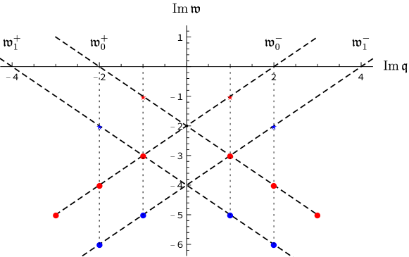
Figure 15: Pole-skipping and level-crossing points in a $2d$ CFT correlator of operators with conformal dimension $\Delta=2$, for the smallest in magnitude poles $\mathfrak{w}_{0}^{\pm}$ and $\mathfrak{w}_{1}^{\pm}$. The red stars at $\mbox{Im}\,\mathfrak{q}=\pm 1$ correspond to the pole-skipping points and the red dots label the critical points of level-crossings of $\mathfrak{w}_{0}^{\pm}$. The blue stars at $\mbox{Im}\,\mathfrak{q}=\pm 2$ correspond to the pole-skipping points and the blue dots label the critical points of level-crossings of $\mathfrak{w}_{1}^{\pm}$.

5.2 BTZ spectrum level-crossing

Since the quasinormal spectrum $\mathfrak{w}_{n}^{\pm}(\mathfrak{q})$ is known explicitly (see eq. (124)), the level-crossing points can be found directly. Such level-crossing points were used above in theories with gapless excitations to determine the radius of convergence of their hydrodynamic series. Considering complex $\mathfrak{q}=|\mathfrak{q}|e^{i\theta}$, we have

$$\mbox{Re}\,\mathfrak{w}_{n}^{\pm} =\pm|\mathfrak{q}|\cos{\theta}\equiv X\,,$$ (137)

$$\mbox{Im}\,\mathfrak{w}_{n}^{\pm} =\pm|\mathfrak{q}|\sin{\theta}-2n-\Delta\equiv Y\,,$$ (138)

and thus the orbits followed by the poles in the complex $\mathfrak{w}$ plane when the phase $\theta$ changes from $0$ to $2\pi$ are circles

$$X^{2}+\left(Y+2n+\Delta\right)^{2}=|\mathfrak{q}|^{2}\,,\qquad n=0,1,2,\ldots\,.$$ (139)

The poles move counter-clockwise and collide on the imaginary axis of $\mathfrak{w}$ (moreover, at integer values of $|\mathfrak{w}|$ if $\Delta$ is an integer). More precisely, two poles collide when $\mathfrak{w}_{n}^{-}=\mathfrak{w}_{m}^{+}$, $m\neq n$, i.e. when (the case $n=0$ or $m=0$ is treated separately below)

$$\mathfrak{q}_{\rm c} =i\left(m-n\right)\,,$$ (140)

$$\mathfrak{w}_{\rm c} =-i\left(m+n+\Delta\right)\,,$$ (141)

$$m,n =1,2,\ldots,\,\text{with}~{}m\neq n\,,$$ (142)

with the first collision occurring for $m=n\pm 1$, i.e. for $\mathfrak{q}_{\rm c}=\pm i$, $\mathfrak{w}_{\rm c}=-i\left(2n+\Delta\pm 1\right)$, $n=1,2,\ldots$. The mode with $n=0$, i.e. $\mathfrak{w}_{0}^{\pm}=\pm\mathfrak{q}-i\Delta$, has only one neighbour, and the critical points correspond to $\mathfrak{w}_{0}^{-}=\mathfrak{w}_{n}^{+}$ (i.e. $\mathfrak{q}_{\rm c}=in$ and $\mathfrak{w}_{\rm c}=-i(n+\Delta)$) or $\mathfrak{w}_{n}^{-}=\mathfrak{w}_{0}^{+}$ (i.e. $\mathfrak{q}_{\rm c}=-in$ and $\mathfrak{w}_{\rm c}=-i(n+\Delta)$, $n=1,2,\ldots$). Thus, the zero mode critical points are

$$\mathfrak{q}_{\rm c} =\pm in\,,$$ (143)

$$\mathfrak{w}_{\rm c} =-i\left(n+\Delta\right)\,,$$ (144)

$$n =1,2,\ldots\,.$$ (145)

The motion of poles in the complex frequency plane and their level-crossings are illustrated for $\Delta=1/8$ and $|\mathfrak{q}|=1$ in fig. 16.

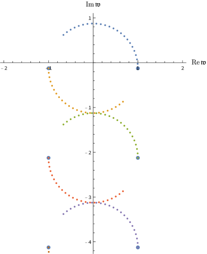
Figure 16: BTZ quasinormal spectrum for $\Delta=1/8$ in the complex $\mathfrak{w}$-plane at complex momentum $\mathfrak{q}=|\mathfrak{q}|e^{i\theta}$, with $|\mathfrak{q}|=1$ and $\theta$ changing from $0$ to $3\pi/4$. The spectrum at $\theta=0$ is shown by large dots.

For larger $|\mathfrak{q}|$, the trajectories intersect but the poles miss each other, so there is no phenomenon of one trajectory crossing into and continuing as the other. In a sense, here, we have “level-touching” rather than “level-crossing”. The nearest critical points are thus

$$\mathfrak{q}_{\rm c} =\pm i\,, \mathfrak{w}_{\rm c} =-i\left(2n+\Delta\pm 1\right)\,, n =1,2,\ldots\,,$$ (146)

$$\mathfrak{q}_{\rm c} =\pm i\,, \mathfrak{w}_{\rm c} =-i\left(\Delta+1\right)\,, n =0\,.$$ (147)

In particular, for $\Delta=2$, we have

$$\mathfrak{q}_{\rm c} =i\,, \mathfrak{w}_{\rm c} =-3i,-5i,-7i,-9i\ldots\,,$$ (148)

$$\mathfrak{q}_{\rm c} =-i\,, \mathfrak{w}_{\rm c} =-3i,-3i,-5i,-7i,\ldots\,.$$ (149)

We observe that for non-integer $\Delta$, the values of $\mathfrak{q}$ corresponding to the pole-skipping and the level-crossing do not coincide. The same is (trivially) true for $\Delta=1$ as well, where there is no pole-skipping in the correlator at all. For $\Delta=2$, however, a curious picture emerges. Consider again the “sound” mode $\mathfrak{w}_{0}^{\pm}$ (136). The imaginary parts of the two branches obey

$$\mbox{Im}\,\mathfrak{w}_{0}^{\pm}=\pm\mbox{Im}\,\mathfrak{q}-2\,.$$ (150)

The pole-skipping points found in section 5.1 are $\mathfrak{q}_{*}=i$, $\mathfrak{w}_{*}=-i$ and $\mathfrak{q}_{*}=-i$, $\mathfrak{w}_{*}=-i$, and the critical points are $\mathfrak{q}_{\rm c}=\pm in$, $\mathfrak{w}_{\rm c}=-i(n+2)$, $n=1,2,\ldots$. For $\Delta=2$, and the mode with $n=1$,

$$\mathfrak{w}_{1}^{\pm}(\mathfrak{q})=\pm\mathfrak{q}-4i\,,$$ (151)

the pole-skipping occurs at $\mathfrak{q}=\pm 2i$ and $\mathfrak{w}=-2i$. The critical points are located at $\mathfrak{q}_{\rm c}=\pm i(m-1)$, $\mathfrak{w}_{\rm c}=-i(m+3)$, $m=2,3,\ldots$. This is illustrated in fig. 15.

6 Discussion

In this paper, we introduced spectral curves as a useful tool for investigating analytic properties of gapless collective excitations in classical hydrodynamics. We showed that the dispersion relations of hydrodynamic modes, such as shear and sound modes, are generically given by Puiseux series expansions in rational powers of the spatial momentum squared. These series are guaranteed to converge in some vicinity of the origin (the point with zero frequency $\omega=0$ and zero spatial momentum ${\bf q}^{2}=0$ in the $(\omega,\mathfrak{q}^{2})\in\mathbb{C}^{2}$ space), so long as the analyticity of the spectral curve at the origin can be proven (e.g. by holographic or other means). Thus, given the analyticity of the spectral curve, the asymptotic nature of the series for hydrodynamic modes in momentum space can be automatically ruled out. The radius of convergence of the series is given by the distance from the origin to the critical point of the spectral curve nearest to the origin. After developing the general theory, we then used holography as a theoretical laboratory where all these of features can be seen and analysed explicitly. Before focusing on the main example of the strongly coupled ${\cal N}=4$ supersymmetric Yang-Mills theory at finite temperature, to illustrate our method, we first considered the holographic model with broken translation symmetry, where an exact spectral curve is available. We have shown that the critical points of the spectral curves can be found by studying quasinormal spectra at complex values of spatial momentum: the critical points correspond to the collisions of quasinormal frequencies (poles of dual correlators) in the complex frequency plane at critical (generically, complex) values of spatial momentum. These values also set the radii of convergence for the dispersion relation. We call this phenomenon the quasinormal mode level-crossing, in analogy with the well-known phenomenon of level-crossing for eigenvalues of Hermitian operators.

Applying these methods to the strongly coupled ${\cal N}=4$ supersymmetric Yang-Mills theory, we found that the gradient expansions for the hydrodynamic shear and sound modes have finite radii of convergence given by $q_{\rm sound}^{\rm c}=\sqrt{2}\,\omega_{0}$ for the sound mode and by $q_{\rm shear}^{\rm c}\approx 1.49\,\omega_{0}$ for the shear mode, where $\omega_{0}=2\pi T$ is the fundamental Matsubara frequency. Thus, in both channels, the hydrodynamic series converge up to the order of $|{\bf q}|/T\sim O(10)$, which is a vast improvement over the naive expectation that $|{\bf q}|/T\ll 1$ provides a natural expansion parameter for hydrodynamic dispersion relations. The obstruction to convergence in the example of the ${\cal N}=4$ SYM theory comes from the collision of poles of the two-point correlation function of the energy-momentum tensor at complex $q^{2}$.

As mentioned in the Introduction, the problem of extending the hydrodynamic modes in the complex momentum plane beyond the branch point singularity was recently investigated by Withers Withers:2018srf in the context of a holographic model in $2+1$ dimensions with finite chemical potential. The shear-diffusion mode series could be Padé-resummed and extended beyond the branch point singularity, which was in that case located at an imaginary value of momentum. The main focus of ref. Withers:2018srf was on the possibility of recovering the full spectrum from the hydrodynamic derivative expansion, similar to recovering the non-hydrodynamic modes from asymptotic series via Borel resummation and resurgence Heller:2013fn ; Heller:2015dha ; Casalderrey-Solana:2017zyh . The quasinormal spectrum in the holographic models with finite temperature $T$ and non-vanishing chemical potential $\mu$ such as the one considered in ref. Withers:2018srf is rather complicated and changes qualitatively as the parameter $T/\mu$ is varied (in particular, it involves pole collisions even at real values of the momentum) Edalati:2010hk ; Edalati:2010pn ; Brattan:2010pq ; Davison:2011uk ; Davison:2011ek ; Gushterov:2018spg ; Gushterov:2018nht . In ref. Withers:2018srf , the shear-diffusion mode was found to have a radius of convergence inversely proportional to the chemical potential. Naively, this would imply infinite radius of convergence in the limit of vanishing $\mu$, in apparent contradiction with our results. However, the result of ref. Withers:2018srf was obtained at a specific fixed value of $T/\mu$, and we expect it to change when the complex momentum behaviour of other gapped modes in the model is taken into account with $T/\mu$ increasing. This will require further study. It would be also interesting to extend the results of the present work to the sound channel (not considered in ref. Withers:2018srf ) as well as to other holographic models with finite chemical potential such as the STU model Son:2006em , and other models Anantua:2012nj , Betzios:2017dol ; Betzios:2018kwn , including those in the large $D$ limit Casalderrey-Solana:2018uag .

Pole collisions in the correlation functions appear in holographic models in different contexts Davison:2011ek ; Davison:2014lua ; Grozdanov:2016vgg ; Grozdanov:2016fkt ; Grozdanov:2018ewh ; Baggioli:2018nnp ; Baggioli:2018vfc ; Grozdanov:2018fic ; Grozdanov:2018gfx ; Gushterov:2018spg ; Davison:2018ofp ; Baggioli:2019jcm . No less interesting are collisions among poles and zeros of the correlators known as pole-skipping Grozdanov:2017ajz ; Blake:2017ris ; Blake:2018leo ; Grozdanov:2018kkt . What we have shown here is that this phenomenon, known to exist in the sound channel of strongly coupled ${\cal N}=4$ SYM theory Grozdanov:2017ajz , exists also in the shear and scalar channels of the energy-momentum correlators. The conjectured connection to the OTOC thus allows one to determine the parameters quantifying microscopic many-body chaos (scrambling time and butterfly velocity) by considering the complexified behaviour of the lowest-lying modes (those with the smallest $|\omega|$ in the spectrum) in any channel, be it a channel with or without hydrodynamic modes. In general, the critical points and the pole-skipping points are different. We have analysed the $2d$ CFT finite-temperature correlators and the spectra of the dual BTZ black hole to demonstrate this explicitly. What this implies for the relation between chaos and hydrodynamics is that the “chaos” (or pole-skipping) points can lie within or outside of the radius of convergence of the hydrodynamic series. In particular, while this is not the case in the holographic model with broken translation symmetry considered in section 3, we found that in the ${\cal N}=4$ SYM theory, pole-skipping points for both of the two hydrodynamic modes lie within the radius of convergence of the corresponding dispersion relations. This provides an explanation for the observation of the fast convergence of the hydrodynamic series to the exact chaos point in ref. Grozdanov:2017ajz .

Can finiteness of the convergence radius of the hydrodynamic modes dispersion relations expansion be taken as a criterion for validity of hydrodynamics? By analogy, one may think of a free particle whose dispersion relation $\omega=\sqrt{p^{2}+m^{2}}-m=p^{2}/2m+\ldots$ has branch points located at $p=\pm im$, and for which the failure of the convergence of the gradient expansion corresponds to the breakdown of the non-relativistic approximation. We hope our results may be of interest for studies of higher-order hydrodynamics necessary for improving the precision of hydrodynamic predictions and also for justifying the construction of the effective field theory of hydrodynamics formulated as a gradient expansion Dubovsky:2011sj ; Grozdanov:2013dba ; Kovtun:2014hpa ; Haehl:2015foa ; Crossley:2015evo ; Haehl:2015uoc ; Glorioso:2016gsa ; Jensen:2017kzi ; Glorioso:2018wxw ; Banks:2018aob ; Chen-Lin:2018kfl . As already mentioned in ref. Grozdanov:2019kge in the context of the discussion of the “unreasonable effectiveness” of hydrodynamics as an effective theory, many previous studies have reported the divergence of the derivative expansion in relativistic hydrodynamics Heller:2013fn ; Heller:2015dha ; Buchel:2016cbj ; Casalderrey-Solana:2017zyh ; Heller:2015dha . Possibly, the asymptotic nature of the expansion appearing in those publications should be viewed as a reflection of the singular nature of the state about which this expansion is performed, rather than a generic property of the hydrodynamic gradient expansion itself. On the other hand, even for a free particle, the momentum space and position space pictures look different in this respect: the small-momentum expansion of the corresponding dispersion relation has a finite radius of convergence, whereas e.g. for the position space propagator, the large-time expansion is only asymptotic. This issue needs further investigation. The role of the non-hydrodynamic degrees of freedom is the common feature of the mentioned works and the present paper.

Of special interest is the dependence of the radii of convergence on coupling. In ref. Grozdanov:2019kge , using eq. (34) as a crude approximation and the results of refs. Buchel:2004di ; Buchel:2008sh , we argued that in the ${\cal N}=4$ SYM theory, the radius of convergence is smaller at weaker coupling. This, of course, requires the actual study of the spectrum at finite coupling. More generally, in the context of the problem of interpolating between weak and strong coupling regimes of the same theory at finite temperature Grozdanov:2016vgg ; Grozdanov:2016zjj , one may note that the problem of convergence of hydrodynamic series has been raised and partially investigated in the 1960s in kinetic theory mclennan . This approach, together with recent studies of relevant issues at weak coupling Romatschke:2015gic ; Kurkela:2017xis ; Moore:2018mma ; Grozdanov:2018atb , may deserve more attention in the context of the problem of the validity of the hydrodynamic description at finite coupling.

Appendix A Analytic implicit function theorem and Puiseux series

Here, we collect the necessary information from complex analysis regarding the following problem. Given an implicit function $f(x,y)=0$, where $x,y\in\mathbb{C}$, we would like to find explicit solution(s) in the form $y=y(x)$, at least locally in the vicinity of some point $(x_{0},y_{0})$, where $y(x)$ may be represented by a finite or infinite series in $x$. We would like to determine, furthermore, what sets the radius of convergence of such series.

A simple example is provided by the function $f(x,y)=x^{2}+y^{2}-1=0$. Since $f(x,y)$ is a polynomial, it determines a complex algebraic curve. Singular points of $f(x,y)$ are determined by the simultaneous solution of the equations $f(x,y)=0$, $f_{,x}(x,y)=0$, $f_{,y}(x,y)=0$, where the comma subscript denotes the partial derivative with respect to the argument after the comma. Clearly, this particular curve has no singular points. It does, however, have the so-called “points of multiplicity 1” or “one-fold points”, where $f_{,x}(x,y)=0$ or $f_{,y}(x,y)=0$ (but not both simultaneously). These are sometimes called critical points. We are interested in the local behaviour of $y=y(x)$ near a critical point defined by the conditions $f(x,y)=0$, $f_{,y}(x,y)=0$. In our example, there are two such points: $(x,y)=(\pm 1,0)$. The series representation $y=y(x)$ in the vicinity of e.g. $(x,y)=(1,0)$ has two branches:

$$y=y_{1}(x)=i\sqrt{2}(x-1)^{\frac{1}{2}}+i2^{-\frac{3}{2}}(x-1)^{\frac{3}{2}}+\cdots\,,$$ (152)

$$y=y_{2}(x)=-i\sqrt{2}(x-1)^{\frac{1}{2}}-i2^{-\frac{3}{2}}(x-1)^{\frac{3}{2}}+\cdots\,.$$ (153)

This is an example of the Puiseux series, i.e. the power series with fractional exponents. These series converge in the circle with the centre at $(x,y)=(1,0)$ and radius $R=2$ which is the distance from $(1,0)$ to the nearest critical point, $(x,y)=(-1,0)$.

One may be interest in the behaviour $y=y(x)$ in the vicinity of a regular point, where $f_{,y}(x,y)\neq 0$, for example, near $(x,y)=(0,1)$ in our example. Here, since $f_{,y}(x,y)\neq 0$, the implicit function theorem guarantees that we can compute the derivatives $y^{\prime}(x)$, $y^{\prime\prime}(x)$ and so on, and represent $y(x)$ by the Taylor series in the vicinity of $x=0$,

$$y=y(x)=1-\frac{x^{2}}{2}-\frac{x^{4}}{8}+\cdots\,.$$ (154)

This series is convergent in the circle of radius $R=1$, determined by the distance from the point $x=0$ to the nearest critical point(s) at $x=\pm 1$.

In general, for an implicit function given by the equation $f(x,y)=0$, where $f(x,y)$ is either a finite polynomial in $x$ and $y$, or an analytic function at a point $(x,y)$ (i.e. a polynomial of an infinite degree), the behaviour at a regular point is governed by the analytic implicit function theorem implicit-function-theorem , and the behaviour in the vicinity of a critical point is determined by the Puiseux theorem. In the former case, $y=y(x)$ is represented by a Taylor series converging in some vicinity of a regular point. In the latter case, it is represented by a Puiseux series converging in some vicinity of a critical point. We now recall some facts from complex analysis gunning-rossi and explain the Puiseux construction walker , wall .

Definition: A function, $f(x,y)$, from a neighbourhood of $(x_{0},y_{0})\in\mathbb{C}^{2}$ to $\mathbb{C}$ is called analytic at $(x_{0},y_{0})$ if near $(x_{0},y_{0})$ it is given by the uniformly convergent power series

$$f(x,y)=\sum\limits_{n,m=0}^{\infty}a_{nm}(x-x_{0})^{n}(y-y_{0})^{m}\,.$$ (155)

Analytic implicit function theorem: If $f(x_{0},y_{0})=0$ and $f_{,y}(x_{0},y_{0})\neq 0$, there exist $\epsilon>0$ and $\delta>0$ so that $\mathbb{D}_{\epsilon}(x_{0})\times\mathbb{D}_{\delta}(y_{0})$ is in the neighbourhood where $f$ is defined, and $g$ is a map of $\mathbb{D}_{\epsilon}(x_{0})$ into $\mathbb{D}_{\delta}(y_{0})$ so that $f(x,g(x))=0$ and for each $x\in\mathbb{D}_{\epsilon}(x_{0})$, $g(x)$ is the unique solution of $f(x,g(x))=0$ with $g(x)\in\mathbb{D}_{\delta}(y_{0})$. Moreover, $g(x)$ is analytic in $\mathbb{D}_{\epsilon}(x_{0})$ and

$$g^{\prime}(x)=-\frac{\frac{\partial f}{\partial x}(x,g(x))}{\frac{\partial f}{\partial y}(x,g(x))}\,.$$ (156)

Similarly, one can compute higher derivatives of $g(x)$ and represent it by a Taylor series around $x=x_{0}$ convergent in $\mathbb{D}_{\epsilon}(x_{0})$. Note that the statements of the theorem are local, e.g. the size of the domain $\mathbb{D}_{\epsilon}(x_{0})$ is unspecified, it is only known that it exists for some $\epsilon>0$. In other words, we know that the radius of convergence of the series of $g(x)$ around $x=x_{0}$ is non-zero but its value is left unspecified. In the example above, we saw that the value of the radius of convergence is determined by the distance from the centre of the expansion $x_{0}$ to the nearest critical point of $f(x,y)$. Note also that the statements of the theorem depend crucially on $f(x,y)$ being an analytic function at $(x_{0},y_{0})$ (in particular, a finite order polynomial in $x$ and $y$).

Now we return to the original problem: for $f(x,y)=0$, where $x,y\in\mathbb{C}$, find explicit solution(s) in the form $y=y(x)$, at least locally in the vicinity of some point $(x_{0},y_{0})$, where $y(x)$ may be represented by series (possibly infinite) at $x=x_{0}$. For simplicity, we set $x_{0}=0$. First, we check $f(0,y)$. If this is a polynomial in $y$ of degree $n$, then the equation $f(0,y)=0$ has $n$ roots $y_{i}$, $i=1,\ldots,n$. There are two possibilities.

Local behaviour at regular points: all the roots $y_{i}$, $i=1,\ldots,n$ of the equation $f(0,y)=0$ are distinct. Then $f_{,y}(0,y_{i})\neq 0$, and the analytic implicit function theorem guarantees the existence of a unique Taylor expansion $y=y(x)$ at $x=0$.

Local behaviour at critical points: the equation $f(0,y)=0$ has multiple roots. For simplicity, let $y_{0}=0$ be such a root. Then we have $f(0,0)=0$, $f_{,y}(0,0)=0$, $(\partial^{2}\!f/\partial y^{2})(0,0)=0,\ldots$ $(\partial^{p}\!f/\partial y^{p})(0,0)\neq 0$, if $y=0$ is a zero of $f(0,y)=0$ of order $p$. We expect $p$ branches of the solutions $y=Y_{j}(x)$, $j=1,\ldots,p$, at $x=0$. They are given by Puiseux series

$$y=Y_{j}(x)=\sum\limits_{k\geq k_{0}}^{\infty}a_{k}x^{\frac{k}{m_{j}}}\,,\qquad j=1,\ldots,p\,,$$ (157)

where $m_{j}$ are positive integers, and $k_{0}$ is a non-negative integer which in general depends on $j$. The exponents $k_{0}/m_{j}$, $(k_{0}+1)/m_{j}$, etc, and the coefficients $a_{k_{0}},a_{k_{0}+1}$, etc, can be determined by the Newton polygon method (1671), as described e.g. in refs. walker , wall . The Puiseux series are converging in some vicinity of the point $x=0$ provided $f(x,y)$ is an analytic function at $(x,y)=(0,0)$ (or a finite polynomial). If some $m_{j}>1$, we necessarily have among those $p$ branches a family of $m_{j}$ solutions of the form

$$y=Y_{l}(x)=\sum\limits_{k\geq k_{0}}^{\infty}a_{k}\left(e^{\frac{2\pi il}{m_{j}}}\right)^{k}\,x^{\frac{k}{m_{j}}}\,,\qquad l=0,1,\ldots,m_{j}-1\,.$$ (158)

As an example, consider the algebraic curve sendra

$$f(x,y)=y^{5}-4y^{4}+4y^{3}+2x^{2}y^{2}-xy^{2}+2x^{2}y+2xy+x^{4}+x^{3}=0\,.$$ (159)

Since $f(0,y)=y^{3}(y-2)^{2}$, the points $(0,0)$ and $(0,2)$ are critical points with multiplicities $3$ and $2$, respectively. We expect $y=y(x)$ to be given by 3 branches of Puiseux series at $(0,0)$ and by 2 branches at $(0,2)$. Applying the Newton polygon method walker , wall , sendra at the point $(0,0)$, we find $m_{1}=m_{2}=2$ and $k_{0}=1$, $m_{3}=1$ and $k_{0}=2$, with appropriate coefficients:

$$y=Y_{1}(x)=i\frac{\sqrt{2}}{2}x^{\frac{1}{2}}-\frac{1}{8}\,x+i\frac{27\sqrt{2}}{128}x^{\frac{3}{2}}-\frac{7}{32}\,x^{2}+\cdots\,,$$ (160)

$$y=Y_{2}(x)=-i\frac{\sqrt{2}}{2}x^{\frac{1}{2}}-\frac{1}{8}\,x-i\frac{27\sqrt{2}}{128}x^{\frac{3}{2}}-\frac{7}{32}\,x^{2}+\cdots\,,$$ (161)

$$y=Y_{3}(x)=-\frac{1}{2}\,x^{2}+\frac{1}{8}\,x^{4}-\frac{1}{8}\,x^{5}+\frac{1}{16}\,x^{6}+\cdots\,.$$ (162)

At the point $(0,2)$, we have 2 branches, as expected:

$$y=Y_{4}(x)=2+\frac{1+i\sqrt{95}}{8}\,x+\cdots\,,$$ (163)

$$y=Y_{5}(x)=2+\frac{1-i\sqrt{95}}{8}\,x+\cdots\,.$$ (164)

Appendix B Perturbative solution of eq. (70)

Here, we list the explicit expressions for the components of the perturbative solution of eq. (70),

$$G_{0}(u)\, =u\,,$$

$$G_{1}(u)\, =\left(\frac{\mathfrak{q}^{2}}{2}-i\mathfrak{w}\right)\left(1-u\right)+i\mathfrak{w}\frac{u}{2}\ln{\frac{1+u}{2}}$$

$$=\left(\frac{\mathfrak{q}^{2}}{2}-i\mathfrak{w}\right)\left(1-u\right)-i\mathfrak{w}\,\frac{u}{2}\,\mbox{Li}_{1}\left(\frac{1-u}{2}\right)\,,$$

$$G_{2}(u)\, =\mathfrak{w}^{2}\left[\frac{u}{2}\,\mbox{Li}_{2}\left(\frac{1-u}{2}\right)+\frac{u}{8}\,\mbox{Li}_{1}^{2}\left(\frac{1-u}{2}\right)+\frac{1+u}{2}\,\mbox{Li}_{1}\left(\frac{1-u}{2}\right)\right]$$

$$+\mathfrak{q}^{2}\,\left(\mathfrak{q}^{2}-\frac{3i\mathfrak{w}}{2}\right)\frac{u}{2}\,\mbox{Li}_{1}\left(\frac{1-u}{2}\right)-\frac{i\mathfrak{w}\mathfrak{q}^{2}}{4}\,\mbox{Li}_{1}\left(\frac{1-u}{2}\right)$$

$$+\mathfrak{q}^{2}\left(\frac{\mathfrak{q}^{2}}{2}-i\mathfrak{w}\right)u\ln{u}+\frac{\mathfrak{q}^{4}}{4}\left(1-u\right)\,,$$

as well as the appropriate boundary values,

$$G_{0}(0)\, =0\,,$$

$$G_{1}(0)\, =-i\mathfrak{w}+\frac{\mathfrak{q}^{2}}{2}\,,$$

$$G_{2}(0)\, =\frac{\mathfrak{q}^{4}}{4}-\frac{i\mathfrak{w}\mathfrak{q}^{2}\ln{2}}{4}+\frac{\mathfrak{w}^{2}\ln{2}}{2}\,,$$

$$G_{3}(0)\, =i\mathfrak{w}^{3}\left(\frac{\pi^{2}}{24}+\ln{2}-\frac{3}{8}\ln^{2}2\right)+\mathfrak{q}^{6}\left(\frac{\ln{2}}{4}-\frac{1}{8}\right)+i\mathfrak{w}\mathfrak{q}^{4}\left(\frac{1}{4}-\frac{\ln 2}{8}\right)$$

$$+\mathfrak{q}^{2}\mathfrak{w}^{2}\left(\frac{\pi^{2}}{48}-\frac{\ln{2}}{2}-\frac{\ln^{2}2}{16}\right)\,,$$

$$G_{4}(0)\, =\mathfrak{q}^{8}\left(-\frac{1}{16}+\frac{\pi^{2}}{64}-\frac{\ln{2}}{8}\right)-\mathfrak{q}^{4}\mathfrak{w}^{2}\left(\frac{\pi^{2}}{96}+\left(12-7\ln{2}\right)\frac{\ln{8}}{96}\right)$$

$$-i\mathfrak{q}^{6}\mathfrak{w}\left(\frac{\pi^{2}}{96}+\left(-5+\ln{4}\right)\frac{\ln{64}}{96}\right)$$

$$+\mathfrak{w}^{4}\left(\left(24-5\ln{2}\right)\frac{\ln^{2}{2}}{48}+\frac{\pi^{2}}{48}\left(-4+\ln{8}\right)-\frac{1}{2}\zeta(3)\right)$$

$$+i\mathfrak{q}^{2}\mathfrak{w}^{3}\left(-\frac{\pi^{2}\ln{2}}{96}+\left(-24+\ln{2}\right)\frac{\ln^{2}{2}}{96}+\frac{3}{16}\zeta(3)\right)\,.$$

Appendix C Kepler’s equation at complex eccentricity

The connection between algebraic curves, their critical points and non-analyticity of associated integrals has an interesting history arnold-nh . Newton proved in “Principia” that every algebraically integrable oval must have singular points: all smooth ovals are algebraically non-integrable (hence the non-analyticity $T\propto a^{3/2}$ in the Kepler’s third law). Moreover, the radius of convergence of the series solving Kepler’s equation is determined by the critical points in the complex eccentricity plane.

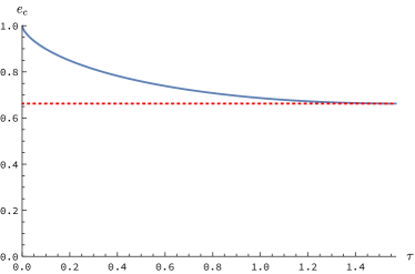
Figure 17: Left panel: Solutions $\psi(\tau)$ of Kepler’s equation (168) at $e=0.75$ for $\tau\in[0,\pi]$ (half a period): “exact” numerical solution of (168) (solid black line), series solution (169) truncated at 50 terms (dashed red line) and 60 terms (dotted blue line). The rate of convergence is maximal at $\tau=\pi/2$. Right panel: The radius of convergence $e_{c}(\tau)$ of the series (169) as a function of $\tau$ for $\tau\in[0,\pi/2]$. The red dotted line coresponds to Laplace’s value $e_{L}$. For $0<e<e_{L}$, the series converges for all $\tau\in[0,2\pi]$.

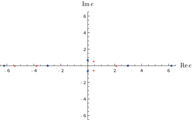
Figure 18: Critical points of the Kepler’s curve (168) in the complex eccentricity plane. The blue dots are the critical points at $\tau=\pi/2$. The points closest to the origin are located at $e\approx\pm 0.662743i$. They determine the radius of convergence $e_{L}$ of the series (169). For $\tau<\pi/2$, the critical points are located at a larger distance from the origin. For example, the critical points at $\tau=\pi/4$ are shown by red asterisks. They determine the radius of convergence $e_{c}(\tau)$, shown in the right panel of fig. 17. With $\tau\rightarrow 0$, the three critical points merge at $e=1$.

Kepler’s law of motion of a planet in an elliptical orbit with eccentricity $e$, $0<e<1$, is usually expressed in a parametric form landau-mechanics

$$r=a\left(1-e\cos{\psi}\right)\,,$$ (165)

$$t=\frac{T}{2\pi}\left(\psi-e\sin{\psi}\right)\,,$$ (166)

where $r$ is the magnitude of the radius-vector from the centre of the force to the planet, $a$ is the major semi-axis of the ellipse, $T$ is the period of revolution and $\psi\in[0,2\pi]$ is the parameter known in astronomy as the eccentric anomaly. Knowing $\psi(t)$, one can find the position of the planet in the polar coordinates $(r(t),\varphi(t))$ as a function of time using Eq. (165) and the equation

$$\tan{\frac{\varphi}{2}}=\sqrt{\frac{1+e}{1-e}}\tan{\frac{\psi}{2}}\,.$$ (167)

Introducing $\tau\equiv 2\pi t/T$, we rewrite Eq. (166) as

$$K=\tau-\psi+e\sin{\psi}=0\,.$$ (168)

Eq. (168) is known as Kepler’s equation. The task of finding a solution $\psi=\psi(\tau)$ preoccupied Kepler, Newton, Lagrange, Laplace, Bessel, Cauchy and other great minds and led to progress in various mathematical disciplines. To quote V.I. Arnold arnold-nh : “This equation plays an important role in the history of mathematics. From the time of Newton, the solution has been sought in the form of a series in powers of the eccentricity $e$. The series converges when $|e|\leq 0.662743...$. The investigation of the origin of this mysterious constant led Cauchy to the creation of complex analysis. Such fundamental mathematical concepts and results as Bessel functions, Fourier series, the topological index of a vector field, and the “principle of the argument” of the theory of functions of a complex variable also first appeared in the investigation of Kepler’s equation”.

A formal series solution of Kepler’s equation was found by Lagrange Lagrange-1771 who apparently was not concerned with the series convergence (more details can be found in the book colwell )

$$\psi(\tau,e)=\tau+\sum\limits_{n=1}^{\infty}\,a_{n}(\tau)\frac{e^{n}}{n!}\,,$$ (169)

where

$$a_{n}=\frac{d^{n-1}(\sin^{n}\tau)}{d\tau^{n-1}}\,.$$ (170)

As pointed out by Laplace Laplace-1823 , the series (169) converges for all $\tau\in[0,2\pi]$ as long as $|e|\leq e_{L}\approx 0.662743...$. For $e>e_{L}$, the series diverges for some values of $\tau$, in a rather peculiar manner (see fig. 17, left panel).

What determines the radius of convergence $e_{c}(\tau)$ of the series (169)? This problem was investigated by Cauchy, Puiseux and Serret in a series of papers in 1849-1859 colwell . In modern language, the answer is the following. Treat Kepler’s equation (168) as a complex analytic curve in the space of $\psi\in\mathbb{C}$, $e\in\mathbb{C}$, with $\tau$ remaining a real parameter. The critical points of the curve $K=0$ obey Eq. (168) as well as the equation

$$\frac{\partial K}{\partial\psi}=e\cos{\psi}-1=0\,.$$ (171)

The critical points closest to the origin in the complex eccentricity plane are shown in fig. 18. Their location is parametrised by $\tau$. The radius of convergence $e_{c}(\tau)$ is given by the distance from the origin to the nearest singularity. This distance is a monotonic function of $\tau$ in the interval $[0,\pi]$ (half a period), with the minimum at $\tau=\pi/2$ given by $e_{c}(\frac{\pi}{2})=e_{L}$. Thus, for $0<e<e_{L}$, the series (169) converges for all $\tau\in[0,2\pi]$. The dependence of the radius of convergence on $\tau$ is shown in fig. 17 (right panel).

References

- (1) L. Landau and E. Lifshits, Fluid Mechanics. Pergamon Press, New York, 1987.
- (2) P. Kovtun, Lectures on hydrodynamic fluctuations in relativistic theories, J. Phys. A45 (2012) 473001 [1205.5040].
- (3) R. Baier, P. Romatschke, D. T. Son, A. O. Starinets and M. A. Stephanov, Relativistic viscous hydrodynamics, conformal invariance, and holography, JHEP 04 (2008) 100 [0712.2451].
- (4) S. Bhattacharyya, Constraints on the second order transport coefficients of an uncharged fluid, JHEP 07 (2012) 104 [1201.4654].
- (5) S. Grozdanov and N. Kaplis, Constructing higher-order hydrodynamics: The third order, Phys. Rev. D93 (2016) 066012 [1507.02461].
- (6) Y. Pomeau and P. Resibois, Time Dependent Correlation Functions and Mode-Mode Coupling Theories, Phys. Rept. 19 (1975) 63.
- (7) M. H. Ernst and J. R. Dorfman, Nonanalytic dispersion relations for classical fluids, Journal of Statistical Physics 12 (1975) 311.
- (8) S. Grozdanov, P. K. Kovtun, A. O. Starinets and P. Tadić, Convergence of the Gradient Expansion in Hydrodynamics, Phys. Rev. Lett. 122 (2019) 251601 [1904.01018].
- (9) T. Kato, Perturbation Theory for Linear Operators. Springer, Berlin, 1980.
- (10) J. D. Baker, D. E. Freund, R. N. Hill and J. D. Morgan III, Radius of convergence and analytic behavior of the expansion, Phys. Rev. A41 (1990) 1247 [1507.02461].
- (11) R. L. Peck, Analysis of the Radius of Convergence of the Perturbation Expansion for the Ground State Energy of Two-Electron Atoms, Electronic Theses and Dissertations, U.Windsor, Canada, 7289 (2017) .
- (12) Y. Bu and M. Lublinsky, All order linearized hydrodynamics from fluid-gravity correspondence, Phys. Rev. D90 (2014) 086003 [1406.7222].
- (13) Y. Bu and M. Lublinsky, Linearized fluid/gravity correspondence: from shear viscosity to all order hydrodynamics, JHEP 11 (2014) 064 [1409.3095].
- (14) A. Kurkela and U. A. Wiedemann, Analytic structure of nonhydrodynamic modes in kinetic theory, 1712.04376.
- (15) A. Buchel, M. P. Heller and J. Noronha, Entropy Production, Hydrodynamics, and Resurgence in the Primordial Quark-Gluon Plasma from Holography, Phys. Rev. D94 (2016) 106011 [1603.05344].
- (16) I. Aniceto, G. Basar and R. Schiappa, A Primer on Resurgent Transseries and Their Asymptotics, 1802.10441.
- (17) M. P. Heller, R. A. Janik and P. Witaszczyk, Hydrodynamic Gradient Expansion in Gauge Theory Plasmas, Phys. Rev. Lett. 110 (2013) 211602 [1302.0697].
- (18) M. P. Heller and M. Spalinski, Hydrodynamics Beyond the Gradient Expansion: Resurgence and Resummation, Phys. Rev. Lett. 115 (2015) 072501 [1503.07514].
- (19) G. Basar and G. V. Dunne, Hydrodynamics, resurgence, and transasymptotics, Phys. Rev. D92 (2015) 125011 [1509.05046].
- (20) I. Aniceto and M. Spaliński, Resurgence in Extended Hydrodynamics, Phys. Rev. D93 (2016) 085008 [1511.06358].
- (21) W. Florkowski, R. Ryblewski and M. Spalinski, Gradient expansion for anisotropic hydrodynamics, Phys. Rev. D94 (2016) 114025 [1608.07558].
- (22) G. S. Denicol and J. Noronha, Divergence of the Chapman-Enskog expansion in relativistic kinetic theory, 1608.07869.
- (23) W. Florkowski, M. P. Heller and M. Spalinski, New theories of relativistic hydrodynamics in the LHC era, 1707.02282.
- (24) M. Spaliński, On the hydrodynamic attractor of Yang-Mills plasma, 1708.01921.
- (25) J. Casalderrey-Solana, N. I. Gushterov and B. Meiring, Resurgence and Hydrodynamic Attractors in Gauss-Bonnet Holography, 1712.02772.
- (26) M. P. Heller and V. Svensson, How does relativistic kinetic theory remember about initial conditions?, Phys. Rev. D98 (2018) 054016 [1802.08225].
- (27) B. Withers, Short-lived modes from hydrodynamic dispersion relations, JHEP 06 (2018) 059 [1803.08058].
- (28) L. P. Kadanoff and P. C. Martin, Hydrodynamic equations and correlation functions, Ann. Phys. 24 (1963) 419.
- (29) S. Grozdanov, K. Schalm and V. Scopelliti, Black hole scrambling from hydrodynamics, Phys. Rev. Lett. 120 (2018) 231601 [1710.00921].
- (30) M. Blake, H. Lee and H. Liu, A quantum hydrodynamical description for scrambling and many-body chaos, JHEP 10 (2018) 127 [1801.00010].
- (31) M. Blake, R. A. Davison, S. Grozdanov and H. Liu, Many-body chaos and energy dynamics in holography, JHEP 10 (2018) 035 [1809.01169].
- (32) S. Grozdanov, On the connection between hydrodynamics and quantum chaos in holographic theories with stringy corrections, JHEP 01 (2019) 048 [1811.09641].
- (33) R. A. Davison and B. Gouteraux, Momentum dissipation and effective theories of coherent and incoherent transport, JHEP 01 (2015) 039 [1411.1062].
- (34) D. T. Son and A. O. Starinets, Minkowski space correlators in AdS / CFT correspondence: Recipe and applications, JHEP 09 (2002) 042 [hep-th/0205051].
- (35) G. Policastro, D. T. Son and A. O. Starinets, From AdS / CFT correspondence to hydrodynamics, JHEP 09 (2002) 043 [hep-th/0205052].
- (36) M. Ammon and J. Erdmenger, Gauge/gravity duality. Cambridge University Press, 2015.
- (37) J. Casalderrey-Solana, H. Liu, D. Mateos, K. Rajagopal and U. A. Wiedemann, Gauge/String Duality, Hot QCD and Heavy Ion Collisions. Cambridge University Press, 2011, 10.1017/CBO9781139136747, [1101.0618].
- (38) J. Zaanen, Y. Liu, Y. Sun and K. Schalm, Holographic Duality in Condensed Matter Physics. Cambridge University Press, 2015.
- (39) S. Hartnoll, A. Lucas and S. Sachdev, Holographic Quantum Matter, The MIT Press. MIT Press, 2018.
- (40) G. Policastro, D. T. Son and A. O. Starinets, From AdS / CFT correspondence to hydrodynamics. 2. Sound waves, JHEP 12 (2002) 054 [hep-th/0210220].
- (41) P. K. Kovtun and A. O. Starinets, Quasinormal modes and holography, Phys. Rev. D72 (2005) 086009 [hep-th/0506184].
- (42) G. Festuccia and H. Liu, A Bohr-Sommerfeld quantization formula for quasinormal frequencies of AdS black holes, Adv. Sci. Lett. 2 (2009) 221 [0811.1033].
- (43) J. F. Fuini, C. F. Uhlemann and L. G. Yaffe, Damping of hard excitations in strongly coupled plasma, JHEP 12 (2016) 042 [1610.03491].
- (44) P. Di Francesco, P. Mathieu and D. Senechal, Conformal Field Theory, Graduate Texts in Contemporary Physics. Springer-Verlag, New York, 1997, 10.1007/978-1-4612-2256-9.
- (45) C. Wall, Singular Points of Plane Curves. Cambridge University Press, Cambridge, 2004.
- (46) P. Kovtun, First-order relativistic hydrodynamics is stable, 1907.08191.
- (47) R. J. Walker, Algebraic Curves. Princeton University Press, Princeton, 1950.
- (48) J. R. Sendra, F. Winkler and S. Pérez-Díaz, Rational Algebraic Curves: A Computer Algebra Approach. Springer, Berlin, 2008.
- (49) P. Kovtun, G. D. Moore and P. Romatschke, The stickiness of sound: An absolute lower limit on viscosity and the breakdown of second order relativistic hydrodynamics, Phys. Rev. D84 (2011) 025006 [1104.1586].
- (50) A. Parnachev and A. Starinets, The Silence of the little strings, JHEP 10 (2005) 027 [hep-th/0506144].
- (51) M. Bhattacharya and C. Raman, Detecting level crossings without looking at the spectrum, Phys. Rev. Lett. 97 (2006) 140405 [physics/0604213].
- (52) T. Andrade and B. Withers, A simple holographic model of momentum relaxation, JHEP 05 (2014) 101 [1311.5157].
- (53) R. C. Myers, A. O. Starinets and R. M. Thomson, Holographic spectral functions and diffusion constants for fundamental matter, JHEP 11 (2007) 091 [0706.0162].
- (54) G. Hardy, Divergent Series. Clarendon Press, 1967.
- (55) D. T. Son and A. O. Starinets, Viscosity, Black Holes, and Quantum Field Theory, Ann. Rev. Nucl. Part. Sci. 57 (2007) 95 [0704.0240].
- (56) A. O. Starinets, Quasinormal modes of near extremal black branes, Phys. Rev. D66 (2002) 124013 [hep-th/0207133].
- (57) S. Grozdanov and A. O. Starinets, Second-order transport, quasinormal modes and zero-viscosity limit in the Gauss-Bonnet holographic fluid, JHEP 03 (2017) 166 [1611.07053].
- (58) A. Nunez and A. O. Starinets, AdS / CFT correspondence, quasinormal modes, and thermal correlators in N=4 SYM, Phys. Rev. D67 (2003) 124013 [hep-th/0302026].
- (59) R. A. Davison and A. O. Starinets, Holographic zero sound at finite temperature, Phys. Rev. D85 (2012) 026004 [1109.6343].
- (60) S. Grozdanov, N. Kaplis and A. O. Starinets, From strong to weak coupling in holographic models of thermalization, JHEP 07 (2016) 151 [1605.02173].
- (61) S. Grozdanov and N. Poovuttikul, Generalized global symmetries in states with dynamical defects: The case of the transverse sound in field theory and holography, Phys. Rev. D97 (2018) 106005 [1801.03199].
- (62) M. Baggioli and K. Trachenko, Maxwell interpolation and close similarities between liquids and holographic models, 1808.05391.
- (63) M. Baggioli and K. Trachenko, Low frequency propagating shear waves in holographic liquids, JHEP 03 (2019) 093 [1807.10530].
- (64) S. Grozdanov, A. Lucas and N. Poovuttikul, Holography and hydrodynamics with weakly broken symmetries, Phys. Rev. D99 (2019) 086012 [1810.10016].
- (65) S. Grozdanov and A. O. Starinets, Adding new branches to the “Christmas tree” of the quasinormal spectrum of black branes, JHEP 04 (2019) 080 [1812.09288].
- (66) N. I. Gushterov, A. O’Bannon and R. Rodgers, Holographic Zero Sound from Spacetime-Filling Branes, JHEP 10 (2018) 076 [1807.11327].
- (67) R. A. Davison, S. A. Gentle and B. Goutéraux, Slow relaxation and diffusion in holographic quantum critical phases, 1808.05659.
- (68) M. Baggioli, V. Brazhkin, K. Trachenko and M. Vasin, Gapped momentum states, 1904.01419.
- (69) S. Bhattacharyya, V. E. Hubeny, S. Minwalla and M. Rangamani, Nonlinear Fluid Dynamics from Gravity, JHEP 02 (2008) 045 [0712.2456].
- (70) Y. Bu, M. Lublinsky and A. Sharon, Hydrodynamics dual to Einstein-Gauss-Bonnet gravity: all-order gradient resummation, JHEP 06 (2015) 162 [1504.01370].
- (71) F. M. Haehl and M. Rozali, Effective Field Theory for Chaotic CFTs, JHEP 10 (2018) 118 [1808.02898].
- (72) D. Birmingham, I. Sachs and S. N. Solodukhin, Conformal field theory interpretation of black hole quasinormal modes, Phys. Rev. Lett. 88 (2002) 151301 [hep-th/0112055].
- (73) M. Blake, R. A. Davison and D. Vegh, Horizon constraints on holographic Green’s functions, 1904.12883.
- (74) S. Datta, P. Kraus and B. Michel, Typicality and thermality in 2d CFT, 1904.00668.
- (75) M. Edalati, J. I. Jottar and R. G. Leigh, Shear Modes, Criticality and Extremal Black Holes, JHEP 04 (2010) 075 [1001.0779].
- (76) M. Edalati, J. I. Jottar and R. G. Leigh, Holography and the sound of criticality, JHEP 10 (2010) 058 [1005.4075].
- (77) D. K. Brattan and S. A. Gentle, Shear channel correlators from hot charged black holes, JHEP 04 (2011) 082 [1012.1280].
- (78) R. A. Davison and N. K. Kaplis, Bosonic excitations of the Reissner-Nordstrom black hole, JHEP 12 (2011) 037 [1111.0660].
- (79) N. I. Gushterov, Quasinormal Modes and Correlators in the Shear Channel of Spacetime-Filling Branes, 1807.11390.
- (80) D. T. Son and A. O. Starinets, Hydrodynamics of r-charged black holes, JHEP 03 (2006) 052 [hep-th/0601157].
- (81) R. J. Anantua, S. A. Hartnoll, V. L. Martin and D. M. Ramirez, The Pauli exclusion principle at strong coupling: Holographic matter and momentum space, JHEP 03 (2013) 104 [1210.1590].
- (82) P. Betzios, U. Gursoy, M. Jarvinen and G. Policastro, Quasinormal modes of a strongly coupled nonconformal plasma and approach to criticality, Phys. Rev. D97 (2018) 081901 [1708.02252].
- (83) P. Betzios, U. Gursoy, M. Jarvinen and G. Policastro, Fluctuations in non-conformal holographic plasma at criticality, 1807.01718.
- (84) J. Casalderrey-Solana, C. P. Herzog and B. Meiring, Holographic Bjorken Flow at Large-, JHEP 01 (2019) 181 [1810.02314].
- (85) S. Dubovsky, L. Hui, A. Nicolis and D. T. Son, Effective field theory for hydrodynamics: thermodynamics, and the derivative expansion, Phys. Rev. D85 (2012) 085029 [1107.0731].
- (86) S. Grozdanov and J. Polonyi, Viscosity and dissipative hydrodynamics from effective field theory, Phys. Rev. D91 (2015) 105031 [1305.3670].
- (87) P. Kovtun, G. D. Moore and P. Romatschke, Towards an effective action for relativistic dissipative hydrodynamics, JHEP 07 (2014) 123 [1405.3967].
- (88) F. M. Haehl, R. Loganayagam and M. Rangamani, The Fluid Manifesto: Emergent symmetries, hydrodynamics, and black holes, JHEP 01 (2016) 184 [1510.02494].
- (89) M. Crossley, P. Glorioso and H. Liu, Effective field theory of dissipative fluids, JHEP 09 (2017) 095 [1511.03646].
- (90) F. M. Haehl, R. Loganayagam and M. Rangamani, Topological sigma models & dissipative hydrodynamics, JHEP 04 (2016) 039 [1511.07809].
- (91) P. Glorioso and H. Liu, The second law of thermodynamics from symmetry and unitarity, 1612.07705.
- (92) K. Jensen, N. Pinzani-Fokeeva and A. Yarom, Dissipative hydrodynamics in superspace, JHEP 09 (2018) 127 [1701.07436].
- (93) H. Liu and P. Glorioso, Lectures on non-equilibrium effective field theories and fluctuating hydrodynamics, PoS TASI2017 (2018) 008 [1805.09331].
- (94) T. Banks and A. Lucas, Emergent entropy production and hydrodynamics in quantum many-body systems, Phys. Rev. E99 (2019) 022105 [1810.11024].
- (95) X. Chen-Lin, L. V. Delacretaz and S. A. Hartnoll, Theory of diffusive fluctuations, Phys. Rev. Lett. 122 (2019) 091602 [1811.12540].
- (96) A. Buchel, J. T. Liu and A. O. Starinets, Coupling constant dependence of the shear viscosity in N=4 supersymmetric Yang-Mills theory, Nucl. Phys. B707 (2005) 56 [hep-th/0406264].
- (97) A. Buchel, Resolving disagreement for eta/s in a CFT plasma at finite coupling, Nucl. Phys. B803 (2008) 166 [0805.2683].
- (98) S. Grozdanov and W. van der Schee, Coupling Constant Corrections in a Holographic Model of Heavy Ion Collisions, Phys. Rev. Lett. 119 (2017) 011601 [1610.08976].
- (99) J. A. McLennan, Convergence of the Chapman-Enskog Expansion for the Linearized Boltzmann Equation, The Physics of Fluids 8 (1965) 1580.
- (100) P. Romatschke, Retarded correlators in kinetic theory: branch cuts, poles and hydrodynamic onset transitions, Eur. Phys. J. C76 (2016) 352 [1512.02641].
- (101) G. D. Moore, Stress-stress correlator in theory: Poles or a Cut?, 1803.00736.
- (102) S. Grozdanov, K. Schalm and V. Scopelliti, Kinetic theory for classical and quantum many-body chaos, 1804.09182.
- (103) S. Krantz and H. Parks, The Implicit Function Theorem: History, Theory, and Applications. Springer, New York, Heidelberg, London, 2013.
- (104) R. C. Gunning and H. Rossi, Analytic Functions of Several Complex Variables. Prentice-Hall, Englewood Cliffs, NJ, 1965.
- (105) V. Arnold, Huygens and Barrow, Newton and Hooke: Pioneers in mathematical analysis and catastrophe theory from evolvents to quasicrystals. Birkhauser Verlag, Berlin, 1990.
- (106) L. Landau and E. Lifshits, Mechanics. Pergamon Press, New York, 1960.
- (107) J. Lagrange, Sur le problème de Kepler, Mémoires de l’Académie Royale des Sciences 25 (1771) 204.
- (108) P. Colwell, Solving Kepler’s equation over three centuries. Willmann-Bell, Richmond, 1993.
- (109) P. Laplace, Mémoire sur le développement de l’anomalie vrai et du rayon-vecteur elliptique, en séries ordonées suivant les puissances de l’excentricité, Mémoires de l’Académie Royale des Sciences 6 (1823) 61.