Anthropic Bound on Dark Radiation and its Implications for Reheating

Abstract

We derive an anthropic bound on the extra neutrino species, $\Delta N_{\rm eff}$, based on the observation that a positive $\Delta N_{\rm eff}$ suppresses the growth of matter fluctuations due to the prolonged radiation dominated era, which reduces the fraction of matter that collapses into galaxies, hence, the number of observers. We vary $\Delta N_{\rm eff}$ and the positive cosmological constant while fixing the other cosmological parameters. We then show that the probability of finding ourselves in a universe satisfying the current bound is of order a few percents for a flat prior distribution. If $\Delta N_{\rm eff}$ is found to be close to the current upper bound or the value suggested by the $H_{0}$ tension, the anthropic explanation is not very unlikely. On the other hand, if the upper bound on $\Delta N_{\rm eff}$ is significantly improved by future observations, such simple anthropic consideration does not explain the small value of $\Delta N_{\rm eff}$. We also study simple models where dark radiation consists of relativistic particles produced by heavy scalar decays, and show that the prior probability distribution sensitively depends on the number of the particle species.

1 Introduction

The $\Lambda$CDM paradigm has been hugely successful in explaining various cosmological observations with high accuracy. Remarkably, with only six parameters, it gives a very nice fit to the observed cosmic microwave background (CMB) temperature and polarization anisotropies [1].

Recently, however, the $\Lambda$CDM paradigm is challenged by the findings of possible tensions among different observations. In particular, there seems to be a rather clear tension in the estimate of the Hubble constant, $H_{0}$, In other words, the Hubble constant measured locally is higher than the value inferred from the Planck CMB observation based on the $\Lambda$CDM model. The recent improved analysis of the local measurements of $H_{0}$ strengthened the tension to be $4.4\sigma$ [2]. While it is not trivial to entirely remove the $H_{0}$ tension by introducing new physics without invoking other tensions, there are several ways that can ameliorate the tension [3, 4, 5, 6, 7, 8, 9, 10, 11, 12, 13, 14]. One of such extensions is to introduce new relativistic particles, the so-called dark radiation. It is customary to express the amount of dark radiation in terms of the extra neutrino species, $\Delta N_{\rm eff}$. One needs $\Delta N_{\rm eff}\gtrsim 0.4-0.5$ to reduce the $H_{0}$ tension significantly [7, 2].

There are a variety of candidates for dark radiation. In most of the scenarios, dark radiation consists of unknown massless or extremely light particles such as sterile neutrinos, axions, hidden photons, etc. The existence (or non-existence) of dark radiation has rich implications for physics beyond the SM as well as the evolution of the early Universe. For instance, if dark radiation was in thermal equilibrium with the standard model (SM) particles, they must have sizable couplings that can be constrained by direct search experiments or astrophysics [15, 16, 17, 18, 19]. On the other hand, dark radiation may be produced non-thermally by the decay of heavy particles (see e.g. Refs. [20, 21, 22, 23, 24]). Indeed, in the string theory, there often appear many light hidden particles (such as axions and hidden photons), and if the inflaton is universally coupled to the light particles including the SM ones, we expect that the Universe is likely filled with hidden particles, which is not consistent with what we observe [25]. Therefore, if the existence of dark radiation is ubiquitous in the landscape, there may be some reason to suppress its abundance.

In this Letter, we examine an anthropic explanation of the dark radiation under the assumption that $\Delta N_{\rm eff}$ is an environmental parameter which takes random values in the multiverse. A similar assumption is made in the anthropic explanation of the observed small cosmological constant [26, 27, 28, 29, 30]. Specifically, we vary both $\Delta N_{\rm eff}$ (or $N_{\rm eff}$) and the positive cosmological constant while fixing the other cosmological parameters. Although we do not give a rigorous UV completion that provides such a mechanism to distribute different values of $\Delta N_{\rm eff}$, it is possible to imagine that the abundances of such light particles depend on their couplings with the inflaton, which may depend on the choice of the universe. We shall study simple toy models along this line, and show that the prior distribution of $\Delta N_{\rm eff}$ sensitively depends on the number of particle species that constitute dark radiation. Since it is notoriously difficult to quantify various anthropic conditions, we will adopt a very simple ansatz which seems to be successful in explaining the observed cosmological constant [30, 31]: the number of observers in a universe is proportional to the fraction of matter that collapses into galaxies. In fact, we note that one can extend the anthropic argument on the cosmological constant to derive the anthropic bound on $\Delta N_{\rm eff}$ and its likely values. In this sense, our anthropic explanation of dark radiation is on the same footing with that of the cosmological constant.

2 Anthropic bound on dark radiation

2.1 Probability distribution of $\Delta N_{\rm eff}$ and $\Omega_{\Lambda}$

The effective neutrino number in the standard cosmology is $N_{\rm eff}^{\rm(std)}\simeq 3.046$. The energy density of dark radiation $\rho_{\rm DR}$ is conveniently described by a change of the effective neutrino number $\Delta N_{\rm eff}\equiv N_{\rm eff}-N_{\rm eff}^{\rm(std)}$ as

$$\Delta N_{\rm eff}=\frac{4}{7}\frac{\rho_{\rm DR}}{(\pi^{2}/30)T_{\nu}^{4}},$$ (2.1)

where $T_{\nu}$ is the neutrino temperature. We can express the radiation density parameter, $\Omega_{\rm rad}$, as a function of $\Delta N_{\rm eff}$:

$$\Omega_{\rm rad}\simeq\Omega_{\rm rad}^{\rm(std)}\times\left(1+0.13\Delta N_{\rm eff}\right),$$ (2.2)

where $\Omega_{\rm rad}^{\rm(std)}\simeq 4.18\times 10^{-5}h^{-2}$ is the radiation density parameter in the standard cosmology.

In this Letter, we calculate the conditional probability distribution of $\Delta N_{\rm eff}$ and the density parameter of the cosmological constant $\Omega_{\Lambda}$ in the multiverse, assuming that the probability is proportional to the number of observers in each universe. It is estimated by [32]

$$P(\Delta N_{\rm eff},\Omega_{\Lambda})\propto P_{\rm prior}(\Delta N_{\rm eff},\Omega_{\Lambda})\int dMn_{\rm G}(\Delta N_{\rm eff},\Omega_{\Lambda},M)N_{\rm obs}(\Delta N_{\rm eff},\Omega_{\Lambda},M),$$ (2.3)

where $n_{\rm G}\,dM$ is the comoving number density of galaxies with mass between $M$ and $M+dM$, and $N_{\rm obs}$ is the number of observers per galaxy with mass $M$ in each universe with $\Delta N_{\rm eff}$ and $\Omega_{\Lambda}$. We define the density parameters as $\Omega_{i}=\rho_{i}/\rho_{c}$ ($i={\rm rad},\Lambda$), where $\rho_{c}$ is the critical density of the present universe, and $\rho_{i}$ is evaluated when the energy density of dark matter in each universe becomes equal to the current density. The prior distribution $P_{\rm prior}$ depends on the production mechanism and will be discussed in the next section.

The number of observers $N_{\rm obs}$ in a galaxy is expected to be proportional to its mass $M$. We assume that $N_{\rm obs}$ is insensitive to $\Delta N_{\rm eff}$ and $\Omega_{\Lambda}$, because $N_{\rm obs}$ is determined locally in galaxies decoupled from cosmic expansion, while $\Delta N_{\rm eff}$ and $\Omega_{\Lambda}$ change only global properties of the universe. We also assume that the integral in Eq. (2.3) is dominated by large galaxies with mass $M\gtrsim M_{\rm G}\sim 10^{12}M_{\odot}$ like the Milky Way. This is because the metals generated by the first-generation stars must be retained in the galaxy for the planetary formation. Under these assumptions, we can rewrite the probability as

$$P(\Delta N_{\rm eff},\Omega_{\Lambda})\propto P_{\rm prior}(\Delta N_{\rm eff},\Omega_{\Lambda})F(M>M_{\rm G},\Delta N_{\rm eff},\Omega_{\Lambda}),$$ (2.4)

where $F$ is the fraction of matter that clusters into galaxies with mass larger than $M_{\rm G}$:

$$F(M>M_{\rm G},\Delta N_{\rm eff},\Omega_{\Lambda})\equiv\int_{M_{\rm G}}^{\infty}dMn_{\rm G}(M)M.$$ (2.5)

This can be estimated by using a spherical collapse model.

The observations of CMB revealed that primordial density perturbations are well approximated by a Gaussian. The time evolution of density perturbations can be studied by the linear perturbation theory. Hence it is reasonable to represent the distribution of density perturbations smoothed over a comoving scale $R$ by

$$P_{\delta}(R,t,\Delta N_{\rm eff},\Omega_{\Lambda})\propto\exp\left[-\frac{\delta^{2}}{2\sigma^{2}(R,t,\Delta N_{\rm eff},\Omega_{\Lambda})}\right],$$ (2.6)

where $\delta=\delta\rho/\rho$ is the matter density perturbation, and $\sigma$ is its variance. Note that the variance grows with time.

We are interested in the comoving scale $R_{\rm G}$ leading to the formation of a galaxy with mass $M_{\rm G}$ where planets and observers are formed. They are related by the mass conservation as

$$R_{\rm G}(M_{\rm G}) = \left(\frac{3M_{\rm G}}{4\pi\rho_{\rm m,0}}\right)^{1/3}$$ (2.7)

$$\simeq 1.3h^{-1}\ {\rm Mpc}\left(\frac{\Omega_{m}h^{2}}{0.12}\right)^{-1/3}\left(\frac{h}{0.7}\right)\left(\frac{M_{\rm G}}{10^{12}M_{\odot}}\right)^{1/3},$$ (2.8)

where $\rho_{\rm m,0}$ and $\Omega_{m}$ are the present matter density and density parameter, respectively, and $h$ is the reduced Hubble constant. $M_{G}$ must be large enough to retain metals synthesized in the first-generation stars for the subsequent formation of planets and life. It is not clear, however, which value of $M_{G}$ is appropriate to use for the present analysis. In the following we adopt $M_{G}=10^{12}M_{\odot}$ as a reference value, which is close to the Milky Way mass. In some case we will also show the results for different values, $M_{G}=10^{6}M_{\odot},10^{9}M_{\odot}$, and $10^{13}M_{\odot}$, roughly corresponding to the masses of globular clusters, dwarf galaxies and galaxy groups, respectively.

2.2 Evolution of density perturbations

The variance of density perturbation smoothed over a scale $R$ is calculated from the power spectrum ${\cal P}_{\delta}(k)$ as

$$\sigma^{2}(R,t,\Delta N_{\rm eff},\Omega_{\Lambda})=\int_{0}^{\infty}\frac{4\pi k^{2}dk}{(2\pi)^{3}}{\cal P}_{\delta}(k)W^{2}(kR),$$ (2.9)

$$W(x)=\frac{\sin x-x\cos x}{x^{3}/3},$$ (2.10)

where

$$\left<\delta(k)\delta^{*}(k^{\prime})\right>=(2\pi)^{3}{\cal P}_{\delta}(k)\delta^{(3)}(k-k^{\prime}),$$ (2.11)

$$\delta(k)=\int d^{3}x\,\delta(\vec{x})e^{i\vec{k}\cdot\vec{x}}.$$ (2.12)

Note that the power spectrum ${\cal P}_{\delta}(k)$ is the Fourier transform of the correlation function for the density perturbation, which is different from $P_{\delta}(R)$ in Eq. (2.6).

From the Poisson equation, the density perturbation $\delta$ can be calculated from the gravitational potential $\Phi$ as

$$\delta(k,t) = \frac{2}{3}\frac{k^{2}a\Phi(k,t)}{\Omega_{m}H_{0}^{2}},$$ (2.13)

The time-evolution and $k$-dependence of $\Phi$ are conveniently factorized as

$$\Phi(k,t)=\frac{9}{10}\Phi_{p}(k)T(\kappa)\frac{D(a)}{a},$$ (2.14)

where $T(\kappa)$ is the transfer function, $D(a)$ is the growth function, and $\Phi_{p}$ is the primordial gravitational potential. The numerical factor $9/10$ represents the evolution of super-horizon modes around the matter-radiation equality. The comoving wavenumber in the unit of a horizon scale at the matter-radiation equality, $\kappa$, is given by

$$\kappa =\frac{\sqrt{2}k}{a_{\rm eq}H(a_{\rm eq})}=\frac{\sqrt{\Omega_{\rm rad}}}{\Omega_{m}}\frac{k}{H_{0}},$$ (2.15)

where $a_{\rm eq}$ ($=\Omega_{\rm rad}/\Omega_{m}$) is the scale factor at the matter-radiation equality. The matter power spectrum is then related to the power spectrum of the primordial curvature perturbation ${\cal P}_{\zeta}$ as

$${\cal P}_{\delta}(k)=\frac{8\pi^{2}}{25}\frac{k}{\Omega_{m}^{2}H_{0}^{4}}{\cal P}_{\zeta}(k)T(\kappa)^{2}D(a)^{2},$$ (2.16)

where

$${\cal P}_{\zeta}(k) \simeq 2.101\times 10^{-9}\left(\frac{k}{k_{\rm pivot}}\right)^{n_{s}-1},$$ (2.17)

with $k_{\rm pivot}=0.05{\rm Mpc}^{-1}$ and $n_{s}\simeq 0.965$ [1].

The transfer function describes the wavenumber dependence and the growth function describes the scale-factor dependence of the gravitational potential. Here we briefly comment on the qualitative features of these functions. The density perturbation corresponding to the scale $R_{\rm G}$ enters the horizon before the matter-radiation equality. It is known that the density perturbation at subhorizon scales grows only logarithmically during the radiation dominated era due to the Meszaros effect. The duration of this effect depends on the scale factor at the matter-radiation equality, $a_{\rm eq}$, and therefore $\delta\propto\ln\Omega_{\rm rad}$, where $\Omega_{\rm rad}$ is related to $\Delta N_{\rm eff}$ through Eq. (2.2). On the other hand, the density perturbation grows as $a$ (i.e., $D(a)\propto a$) during the matter dominated epoch. For larger $\Omega_{\rm rad}$, the matter-radiation equality is delayed, and the duration of the matter-dominated epoch decreases. Hence the density perturbation grows less until the present epoch. Combining these effects, we obtain $\delta\propto(\ln\Omega_{\rm rad})/\Omega_{\rm rad}$. Below we will estimate $\delta$ (or $\sigma$) quantitatively and will see the result is consistent with this qualitative picture.

The fitting formula for the transfer function can be read from, e.g., Eq. (6.5.12) in Ref. [34]:

$$T(\kappa) =\frac{\ln\left(1+(0.124\kappa)^{2}\right)}{(0.124\kappa)^{2}}\sqrt{\frac{1+(1.257\kappa)^{2}+(0.4452\kappa)^{4}+(0.2197\kappa)^{6}}{1+(1.606\kappa)^{2}+(0.8568\kappa)^{4}+(0.3927\kappa)^{6}}}.$$ (2.18)

For the modes that enter the horizon before the matter-radiation equality, i.e., $\kappa\gg 1$, we obtain $T(\kappa)\propto\ln\kappa/\kappa^{2}$. The logarithmic dependence results from the Meszaros effect.

It is convenient to define a new time variable $x$ as

$$x\equiv\frac{\rho_{\Lambda}}{\rho_{m}(t)}=\frac{\Omega_{\Lambda}}{\Omega_{m}}(1+z)^{-3}.$$ (2.19)

At the matter-radiation equality, it is given by

$$x_{\rm eq}^{-1/3}=\left(x_{\rm eq}^{(\rm obs)}\right)^{-1/3}\left(\frac{\Omega_{\Lambda}}{\Omega_{\Lambda}^{(\rm obs)}}\right)^{-1/3}\left(\frac{\Omega_{\rm rad}}{\Omega_{\rm rad}^{(\rm std)}}\right)^{-1},$$ (2.20)

and $(x_{\rm eq}/x)^{-1/3}=(a_{\rm eq}/a)^{-1}$, where $(x_{\rm eq}^{(\rm obs)})^{-1/3}\simeq 2820$ and $\Omega_{\Lambda}^{(\rm obs)}\simeq 0.69$ [1]. The growth factor $D(a)$ is given by [33]

$$D(a)=\frac{2a_{\rm eq}}{3}\left[1+\frac{3}{2}x_{\rm eq}^{-1/3}G(x)\right],$$ (2.21)

where $G(x)$ is the growth factor in a flat universe filled with matter and vacuum energy, given by

$$G(x) \equiv \frac{5}{6}\left(\frac{1+x}{x}\right)^{1/2}\int_{0}^{x}\frac{dx^{\prime}}{x^{\prime 1/6}(1+x^{\prime})^{3/2}},$$ (2.22)

$$\approx x^{1/3}\left(1+\left(\frac{x}{G^{3}(\infty)}\right)^{\alpha}\right)^{-1/(3\alpha)}.$$ (2.23)

Here the second line is a fitting formula with

$$\alpha=\frac{159}{200}=0.795,$$ (2.24)

$$G(\infty)=\frac{5\Gamma(2/3)\Gamma(5/6)}{3\sqrt{\pi}}\simeq 1.44.$$ (2.25)

For the scales of our interest, we can safely neglect the first term in Eq. (2.21).

The variance of the density perturbation after smoothing over a scale $R$ (see Eq. (2.9)) is now given by

$$\sigma^{2}(R,t,\Delta N_{\rm eff},\Omega_{\Lambda})=\int_{0}^{\infty}d\ln k{\cal P}_{\zeta}(k)W^{2}(kR)\frac{4}{25}\frac{k^{4}T^{2}(\kappa)}{\Omega_{m}^{2}H_{0}^{4}}D^{2}(a),$$ (2.26)

where ${\cal P}_{\zeta}(k)$, $T(\kappa)$, and $D(a)$ are given by Eqs. (2.17), (2.18), and (2.21), respectively. The dependence of the variance on the parameters can be read by setting $k=1/R_{\rm G}$ in the integrand, and it reads

$$\sigma(R,t,\Delta N_{\rm eff},\Omega_{\Lambda})_{t\to\infty}$$

$$\simeq\sigma^{(\rm std)}(R_{\rm G})\left(1+0.18\ln\frac{\Omega_{\rm rad}}{\Omega_{\rm rad}^{\rm(std)}}\right)\left(\frac{\Omega_{\Lambda}}{\Omega_{\Lambda}^{(\rm obs)}}\right)^{-1/3}\left(\frac{\Omega_{\rm rad}}{\Omega_{\rm rad}^{(\rm std)}}\right)^{-1}\left(\frac{G(\infty)}{G(x_{p})}\right),$$ (2.27)

where

$$\sigma^{(\rm std)}(R_{\rm G})\equiv\sigma(R_{\rm G},t_{p},\Delta N_{\rm eff}=0,\Omega_{\Lambda}^{\rm(obs)})\simeq 3.2,$$ (2.28)

is the variance at present ($t=t_{p}$) evaluated by the linear theory, Eq. (2.26), and $x_{p}\equiv\Omega_{\Lambda}^{(\rm obs)}/\Omega_{m}$. The parameter dependence can be understood by noting how the duration of matter domination depends on the density parameters. That is to say, the matter radiation equality is delayed if we increase the radiation energy. The cosmological constant comes to dominate earlier if we increase the cosmological constant. Since the matter density fluctuation grows efficiently only in the matter dominated epoch, the increase of the density parameters $\Omega_{\rm rad}$ and $\Omega_{\Lambda}$ suppress the growth of the density perturbations. The logarithmic dependence on $\Omega_{\rm rad}$ is due to the Meszaros effect.

2.3 Anthropic bound

When the density perturbation grows and exceeds the critical value $\delta_{c}$, an overdense region collapses to form a galaxy. The critical value can be calculated based on the spherical collapse model [30] (see also Ref. [35]):

$$\delta_{c}\simeq\frac{9}{5}2^{-2/3}G_{\infty}\simeq 1.63.$$ (2.29)

According to [31], the fraction of matter that collapses into galaxies during the entire history of the Universe, $F$, is given by

$$F(M>M_{\rm G},\Delta N_{\rm eff},\Omega_{\Lambda})\propto\int_{\beta}^{\infty}dy\frac{e^{-y}}{s\sqrt{y}+\sqrt{\beta}},$$ (2.30)

where the parameter $\beta$ is given by

$$\beta\equiv\frac{\delta_{c}^{2}}{2\sigma^{2}(R_{\rm G},t,\Delta N_{\rm eff},\Omega_{\Lambda})_{t\to\infty}}\,.$$ (2.31)

Here, $s$ is a shape parameter that takes account of the fraction of the surrounding underdense region that also collapses into the galaxies. If we set $s\to\infty$, the result is proportional to the one given by the Press-Schechter formalism. We take $s=1$, which is a reasonable case where the overdense region is surrounded by the underdense region with the same volume.

Assuming that the number of observers in a universe is proportional to the mass that collapses into galaxies, we can calculate the probability distribution of $\Delta N_{\rm eff}$ and $\Omega_{\Lambda}$ by using Eq. (2.4) and Eq. (2.30). The integral in Eq. (2.30) is exponentially suppressed for $\beta\gg{\cal O}(1)$. This means that the fraction of matter that clusters into galaxies with $M>M_{\rm G}$ is exponentially suppressed for $\sigma\ll\delta_{c}$, while it is of order unity for $\sigma\gtrsim\delta_{c}$. Roughly speaking, the condition $\sigma\gtrsim\delta_{c}$ is the anthropic bound. Since $\sigma$ depends on $\Delta N_{\rm eff}$ and $\Omega_{\Lambda}$, we can estimate their likely values that satisfy $\sigma\gtrsim\delta_{c}$. From the simplified expression Eq. (2.27), we can see that $\Omega_{\Lambda}$ and $\Omega_{\rm rad}(\Delta N_{\rm eff})$ cannot be much larger than the observed values from the anthropic argument.

The normalized probability distribution of $\Delta N_{\rm eff}$ and $\Omega_{\Lambda}$ is shown in Fig. 1. Here we assume a flat prior distribution $P_{\rm prior}$ for both $\Delta N_{\rm eff}$ and $\Omega_{\Lambda}$ in Eq. (2.4) and set $M_{G}=10^{12}M_{\odot}$ as a reference value. In the upper panel, we show a contour plot of $\log[\Omega_{\Lambda}\Delta N_{\rm eff}P(\Delta N_{\rm eff},\Omega_{\Lambda})]$. One can see that the most likely values of $\Delta N_{\rm eff}$ and $\Omega_{\Lambda}$ are larger than those in our universe. In the lower panel, we plot the probability distribution $\Delta N_{\rm eff}P(\Delta N_{\rm eff},\Omega_{\Lambda}^{(\rm obs)})$ as a function of $\Delta N_{\rm eff}$, where the blue solid line is based on the numerical estimate of Eq. (2.26), while the red dashed line is based on the analytic one Eq. (2.27). The two lines agree well with each other. One can also see that the typical value of $\Delta N_{\rm eff}$ is ${\cal O}(10)$.

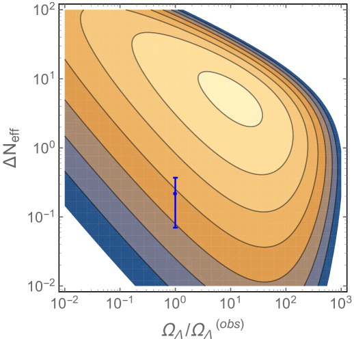
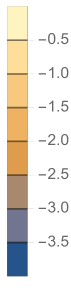
Figure 1: The probability distribution of parameters $\Delta N_{\rm eff}$ and $\Omega_{\Lambda}$ in the multiverse with a flat prior distribution, $P_{\rm prior}=1$. In the upper panel, we show a contour plot of $\log[\Omega_{\Lambda}\Delta N_{\rm eff}P(\Delta N_{\rm eff},\Omega_{\Lambda})]$. In the lower panel, we show the normalized differential probability at $\Omega_{\Lambda}=\Omega_{\Lambda}^{(\rm obs)}$. The blue solid line corresponds to $M_{G}=10^{12}M_{\odot}$. The dotted lines correspond to $M_{G}=10^{6}M_{\odot}$, $10^{9}M_{\odot}$, and $10^{13}M_{\odot}$, respectively from right to left. The red dashed line is based on the simplified expression Eq. (2.27) with $M_{G}=10^{12}M_{\odot}$, which is in good agreement with the blue solid one.

The Planck data combined with the BAO observation gives the constraint [1]

$$N_{\rm eff} =3.27\pm 0.15,$$ (2.32)

which is shown as the blue dot with an error bar in the upper panel of Fig .1. Interestingly, there is currently the so-called $H_{0}$ tension: the Hubble constant inferred by the Planck and BAO (assuming $\Delta N_{\rm eff}=0$) reads $H_{0}=(69.32\pm 0.97)\ {\rm km/s/Mpc}$, while the local Hubble parameter measurement gives $H_{0}=(74.03\pm 1.42)\ {\rm km/s/Mpc}$ [2]. The significance of the tension is greater than $4\sigma$. In fact, $N_{\rm eff}$ and $H_{0}$ are correlated with each other in the Planck analysis; $\Delta N_{\rm eff}>0$ makes the sound horizon smaller, which can be partially cancelled by larger $H_{0}$ because the last scattering surface becomes closer to us. The tension can be relaxed if $\Delta N_{\rm eff}\gtrsim 0.4-0.5$. The $H_{0}$ tension may hint at a sizable amount of dark radiation.

Now we shall discuss how likely the point $\Delta N_{\rm eff}=0.5$ $(1)$ and $\Omega_{\Lambda}=\Omega_{\Lambda}^{(\rm obs)}$ are under the anthropic consideration. First, we note that the probability of finding ourselves in a universe with the present $\Omega_{\Lambda}^{(\rm obs)}$ or smaller is about $3\%$ for the case of $\Delta N_{\rm eff}=0$. We define the probability $\Delta N_{\rm eff}\leq\Delta N_{\rm eff}^{(\rm max)}$ for $\Omega_{\Lambda}=\Omega_{\Lambda}^{(\rm obs)}$ by

$$N^{-1}\int_{0}^{\Delta N_{\rm eff}^{(\rm max)}}d\Delta N_{\rm eff}P(\Delta N_{\rm eff},\Omega_{\Lambda}^{(\rm obs)}),$$ (2.33)

where

$$N=\int_{0}^{\infty}d\Delta N_{\rm eff}P(\Delta N_{\rm eff},\Omega_{\Lambda}^{(\rm obs)}).$$ (2.34)

Then we find that the probability to find ourselves in a universe with $\Delta N_{\rm eff}\leq 0.5$ $(1)$ is about $0.03$ ($0.06$). See also the lower panel of Fig. 1. Thus we conclude that $\Delta N_{\rm eff}=0.5$ (or $1$) is not unlikely based on the anthropic argument.

When we vary both $\Delta N_{\rm eff}$ and $\Omega_{\Lambda}$, the probability to find ourselves in a universe with $\Delta N_{\rm eff}\leq\Delta N_{\rm eff}^{(\rm max)}$ and $0<\Omega_{\Lambda}\leq\Omega_{\Lambda}^{(\rm obs)}$ is given by

$$\int_{0}^{\Delta N_{\rm eff}^{(\rm max)}}d\Delta N_{\rm eff}\int_{0}^{\Omega_{\Lambda}^{(\rm obs)}}d\Omega_{\Lambda}P(\Delta N_{\rm eff},\Omega_{\Lambda}).$$ (2.35)

We find that this is about $0.003$ ($0.006$) for $\Delta N_{\rm eff}^{(\rm max)}=0.5(1)$ and $\Omega_{\Lambda}^{(\rm obs)}=0.69.$

The probability distributions for $M_{G}=10^{6}M_{\odot},10^{9}M_{\odot}$, and $10^{13}M_{\odot}$ are also shown as dotted lines from right to left in the lower panel of Fig. 1. One can see that the probability to find small values of $\Delta N_{\rm eff}$ increases as $M_{G}$ increases. Specifically, we find that the probability to find ourselves in a universe with $\Delta N_{\rm eff}\leq 0.5$ $(1)$ is about $0.01$ ($0.02$) for $M_{G}=10^{6}M_{\odot}$, $0.015$ ($0.03$) for $M_{G}=10^{9}M_{\odot}$ and $0.04$ ($0.07$) for $M_{G}=10^{13}M_{\odot}$.

The CMB-S4 experiment will improve the $1\sigma$ error for the dark radiation as $\delta(N_{\rm eff})=0.0156$ [36, 37]. If the value of $\Delta N_{\rm eff}$ in our universe is determined by the anthropic principle, we would expect that the CMB-S4 experiment will find a nonzero value of $\Delta N_{\rm eff}$ close to the current upper bound. On the other hand, if its result is consistent with $\Delta N_{\rm eff}=0$, we may conclude that the amount of dark radiation is not determined by the anthropic principle but is determined by some other mechanism. For example, the energy of inflation may dominantly converted to the SM particles at the time of reheating.

Finally, we comment on the anthropic bound on the number of neutrino flavors $N_{\rm eff}$ instead of $\Delta N_{\rm eff}$. The effective number of neutrinos $N_{\rm eff}$ can be smaller than the value in the standard cosmology, $N_{\rm eff}^{(\rm std)}\simeq 3.046$, if the rehearing temperature is comparable to or lower than the neutrino decoupling temperature [38, 39, 40, 41]. We can also consider a case in which a low-energy effective theory which is similar to the standard model but with a different number of generations is realized in the multiverse, and the number of generations may be considered as an environmental parameter. In the latter case, $N_{\rm eff}$ will be close to an integer number corresponding to the number of generations (if there is no dark radiation). Motivated by such possibilities, we vary $N_{\rm eff}$ and $\Omega_{\Lambda}$ assuming the flat prior distribution. In Fig. 2 we show the probability distribution of $N_{\rm eff}$ and $\Omega_{\Lambda}$ in the linear plot . We find that the probability to find ourselves in a universe with $N_{\rm eff}\leq 3$ is about $0.15$. Thus, the universe with three neutrino flavors is not unlikely at all based on the anthropic argument, if the prior distribution is flat.

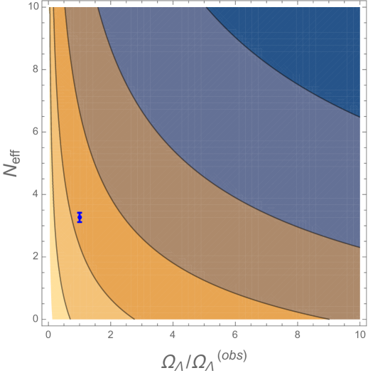
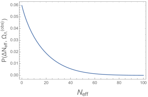
Figure 2: Same as Fig. 1 but with a linear plot for $N_{\rm eff}$ (instead of $\Delta N_{\rm eff}$) and $\Omega_{\Lambda}$. We set $M_{G}=10^{12}M_{\odot}$.

3 Reheating and prior distribution

In this section, we discuss a couple of simple models that predict dark radiation from reheating. Suppose that the inflaton decays into dark radiation as well as the SM particles and that the dark radiation is completely decoupled from the SM sector. The extra neutrino species, which is proportional to the energy density of dark radiation, is then determined by the branching ratio into the dark radiation:

$$\Delta N_{\rm eff}=\frac{43}{7}\left(\frac{43/4}{g_{*}}\right)^{1/3}\frac{\Gamma_{D}}{\Gamma_{\rm SM}},$$ (3.1)

Here, we denote by $g_{*}$ ($\simeq 106.75$) the number of degrees of freedom of the SM particles at the time of reheating. The prior distribution of $\Delta N_{\rm eff}$ is then given by the probability distribution of $\Gamma_{D}/\Gamma_{\rm SM}$.

3.1 Case of a single dark radiation component

In superstring theories, scalar fields with flat potentials, called moduli, arise via compactifications on a Calabi-Yau space, and some of them may be present in the low energy effective field theory [42]. Inflation may be realized in the moduli space, and the decay of the inflaton induces the reheating. Alternatively, coherent oscillations of moduli may dominate the energy density of the Universe after inflation and the subsequent moduli decay reheats the Universe. In either case the reheating occurs due to the moduli decay. In this section we focus on a single modulus that dominates the universe and decays into the SM and dark radiation.

The modulus $T$ has a shift symmetry along its imaginary component, the axion, which remains massless at the perturbative level. We assume that the axion is almost massless, and so, once it is produced it contributes to dark radiation. This is the case if the real component of the modulus is stabilized by supersymmetry breaking effects. Let us consider the following Kähler potential of the no-scale form:

$$K=-3\log\left[T+T^{\dagger}-\frac{1}{3}\left(\left|{H_{u}}\right|^{2}+\left|{H_{d}}\right|^{2}+\left(c_{\rm SM}H_{u}H_{d}+{\rm h.c.}\right)\right)\right]+\dots,$$ (3.2)

where we show only relevant terms and omit higher order terms responsible for e.g. the modulus stabilization, and $c_{\rm SM}$ denotes a coupling constant. For simplicity, we assume that the superpotential and the gauge kinetic function are irrelevant for the modulus decay. Then the modulus decays only into the axion and the Higgs fields. The ratio of the decay rate is given by [21, 22, 23]

$$\frac{\Gamma_{D}}{\Gamma_{\rm SM}}=\frac{1}{2c_{\rm SM}^{2}}.$$ (3.3)

For a more generic Kähler potential, the modulus decay rate into axions is proportional to $(\partial^{3}K/\partial T^{3})^{2}$ ($\equiv c^{2}$), which may vary depending on the details of the compactification etc. So let us parametrize the ratio as

$$\frac{\Gamma_{D}}{\Gamma_{\rm SM}}=\frac{c^{2}}{c_{\rm SM}^{2}},$$ (3.4)

where we take $c_{\rm SM}={\cal O}(0.1)$.

We assume that the coupling constant $c$ that determines $\Gamma_{D}$ is randomly distributed in the multiverse and its probability distribution is given by a flat distribution in the range of $\left|{c}\right|\leq\sigma$ ($={\cal O}(1)$). We fix the decay rate into the SM particles for simplicity. Since the branching ratio into the dark sector is proportional to the coupling constant squared, the probability distribution of $\Gamma_{D}$ can be read from

$$P(c^{2}/\sigma^{2})=\left\{\begin{array}[]{ll}\frac{1}{2\sqrt{c^{2}/\sigma^{2}}}&~{}~{}~{}~{}{\rm for}~{}~{}c^{2}/\sigma^{2}\leq 1\\ 0&~{}~{}~{}~{}{\rm for}~{}~{}c^{2}/\sigma^{2}>1,\end{array}\right.$$ (3.7)

and is proportional to $1/\sqrt{\Gamma_{D}}\propto 1/\sqrt{\Delta N_{\rm eff}}$ for $c^{2}/\sigma^{2}\leq 1$. Thus the distribution of $\Delta N_{\rm eff}$ is biased toward a smaller value. The probability distribution of $\Delta N_{\rm eff}$ and $\Omega_{\Lambda}$ is shown in Fig. 3 for the case of $P_{\rm prior}\propto 1/\sqrt{\Delta N_{\rm eff}}$. We can see that the typical value of $\Delta N_{\rm eff}$ is ${\cal O}(1)$ in this case. The probability to obtain $\Delta N_{\rm eff}\leq 0.5(1)$ is given by $0.10(0.14)$ based on Eq. (2.33). If we also vary $\Omega_{\Lambda}$, the probability to obtain $\Delta N_{\rm eff}\leq 0.5(1)$ and $\Omega_{\Lambda}\leq 0.69$ is $0.01(0.02)$ based on Eq. (2.35).

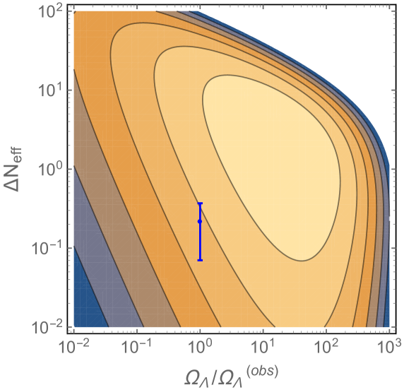
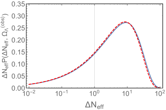
Figure 3: Same as Fig. 1 but with $P_{\rm prior}\propto 1/\sqrt{\Delta N_{\rm eff}}$.

3.2 Case of multiple dark radiation components

We now consider how the probability distribution changes if there are multiple dark radiation components. In fact, the flux compactification of the higher-dimensional space in the string theory predicts a large number of axions and gauged dark sectors in the low-energy effective field theory. Inflation may occur in the axion field space, the so-called axion landscape [43, 44, 45, 46, 47, 48]. For instance, the reheating could occur via the decay into gauge fields. If there are unbroken U(1) gauge fields in the dark sector, they contribute to dark radiation after the reheating. In this case, the number of particle species of the dark radiation, $N$, can be larger than unity [49] and we parametrize the branching into the dark sector as

$$\frac{\Gamma_{D}}{\Gamma_{\rm SM}}=\frac{\sum_{i}c_{i}^{2}}{c_{\rm SM}^{2}}.$$ (3.8)

As in the previous case, we assume that the probability distributions of coupling constants $c_{i}$ are given by flat distributions in the ranges of $\left|{c_{i}}\right|\leq\sigma_{i}$ ($={\cal O}(1)$). For simplicity, we set a universal value for the range, $\sigma_{i}=\sigma$. We also define $x\equiv\sum_{i}c_{i}^{2}/\sigma^{2}\propto\Gamma_{D}$. Since $\Delta N_{\rm eff}\gtrsim{\cal O}(100)$ for $\sum c_{i}^{2}\gtrsim 1$ and $c_{\rm SM}={\cal O}(0.1)$, we are interested in the regime where $x\ll 1$. The probability distribution of $x$ is then calculated from

$$P(x) = \left.\frac{d}{dx}\int_{-\sigma}^{\sigma}\frac{dc_{1}}{2\sigma}\cdots\int_{-\sigma}^{\sigma}\frac{dc_{N}}{2\sigma}\right|_{x<\sum_{i}c_{i}^{2}/\sigma^{2}}$$ (3.9)

$$\simeq \frac{\pi^{N/2}}{2^{N}\Gamma(N/2)}x^{N/2-1}\qquad{\rm for}\ x\leq 1.$$ (3.10)

Thus the prior distribution is almost flat for $N=2$, while it is strongly biases toward a large $\Delta N_{\rm eff}$ for $N>2$. In this case, the probability to obtain $\Delta N_{\rm eff}\leq 0.5$ is strongly suppressed. Thus we conclude that the anthropic argument does not explain the current bound on $\Delta N_{\rm eff}$, if the dark radiation that consists of $N(\gg 1)$ different particle species produced by the heavy scalar decay.

If one assumes that the probability distributions of the coupling constants $c_{i}$ are given by Gaussian distributions with zero mean and a universal variance $\sigma$, the probability distribution of $x\equiv\sum_{i}c_{i}^{2}/\sigma^{2}$ ($\propto\Gamma_{D}$) is then given by the $\chi^{2}$-distribution with $N$ degrees of freedom:

$$P(x)=\chi^{2}(N)=\frac{1}{2^{N/2}\Gamma(N/2)}x^{N/2-1}e^{-x/2}.$$ (3.11)

Note that the result for the case of a single dark radiation component can be read from this formula by setting $N=1$. For a small $x$, the probability distribution is proportional to $x^{N/2-1}$. Since we are interested in a small $x$, the result is the same with that for the flat distribution.

4 Discussion and Conclusions

We have discussed the anthropic bound on the amount of dark radiation, assuming that the number of observers in each universe is proportional to the fraction of matter that clusters into galaxies with mass larger than the Milky Way galaxy. The matter-radiation equality is delayed if we increase the radiation energy. The matter density at subhorizon scales grows only logarithmically before the matter-radiation equality while it grows linearly in terms of the scale factor after that until the cosmological constant comes to dominate. As a result, larger radiation energy leads to smaller density perturbations and hence a lower fraction of matter that clusters into galaxies. We have found that the number of observers is exponentially suppressed when the extra effective neutrino number exceeds of order $10$. If the prior distribution is flat, the probability to find ourselves in a universe with $\Delta N_{\rm eff}\leq 0.5(1)$ is about $0.03(0.06)$, which is comparable to the probability to find ourselves in a universe with the observed cosmological constant or smaller. Therefore, the anthropic explanation of $\Delta N_{\rm eff}$ is not unlikely, if it is found to be around the current upper bound. We have also found that the probability to find ourselves in a universe with less than or equal to three neutrino flavors is about $0.15$ assuming the flat prior distribution in the multiverse.

We have also discussed a couple of examples in which dark radiation is produced during the reheating process. If a modulus is the inflaton or coherent oscillations of the modulus comes to dominate the universe after inflation, the universe will be reheated by the modulus decay. The modulus may also decay into dark radiation in addition to the SM particles. For instance, if the modulus is stabilized by supersymmetry breaking effects, the modulus generically decays into its axionic partners with a sizable branching fraction [21, 22, 23, 24]. Alternatively, the modulus may decay into multiple dark photons or axions. Assuming a flat prior distributions for the coupling constants, we have found that the prior distribution of $\Delta N_{\rm eff}$ is proportional to $(\Delta N_{\rm eff})^{N/2-1}$, where $N$ is the number of particle species that constitute dark radiation. In particular, if $N=1$, the energy density is biased toward smaller values and the probability to find ourselves in a universe with $\Delta N_{\rm eff}\leq 0.5(1)$ is about $0.10(0.14)$. On the other hand, for $N\gg 1$, the prior distribution of $\Delta N_{\rm eff}$ is strongly biased toward larger values. In this case, the probability to find ourselves in a universe with $\Delta N_{\rm eff}\lesssim 1$ is strongly suppressed. In the latter case, some mechanism to dominantly reheat the SM sector may be required.

References

- [1] Planck collaboration, N. Aghanim et al., Planck 2018 results. VI. Cosmological parameters, 1807.06209.
- [2] A. G. Riess, S. Casertano, W. Yuan, L. M. Macri and D. Scolnic, Large Magellanic Cloud Cepheid Standards Provide a 1% Foundation for the Determination of the Hubble Constant and Stronger Evidence for Physics Beyond LambdaCDM, 1903.07603.
- [3] J. Renk, M. Zumalacárregui, F. Montanari and A. Barreira, Galileon gravity in light of ISW, CMB, BAO and H0 data, JCAP 1710 (2017) 020 [1707.02263].
- [4] N. Khosravi, S. Baghram, N. Afshordi and N. Altamirano, üCDM: tension as a hint for Über-Gravity, 1710.09366.
- [5] K. Aylor, M. Joy, L. Knox, M. Millea, S. Raghunathan and W. L. K. Wu, Sounds Discordant: Classical Distance Ladder & CDM -based Determinations of the Cosmological Sound Horizon, Astrophys. J. 874 (2019) 4 [1811.00537].
- [6] S. Dhawan, S. W. Jha and B. Leibundgut, Measuring the Hubble constant with Type Ia supernovae as near-infrared standard candles, Astron. Astrophys. 609 (2018) A72 [1707.00715].
- [7] E. Mörtsell and S. Dhawan, Does the Hubble constant tension call for new physics?, JCAP 1809 (2018) 025 [1801.07260].
- [8] F. D’Eramo, R. Z. Ferreira, A. Notari and J. L. Bernal, Hot Axions and the tension, JCAP 1811 (2018) 014 [1808.07430].
- [9] C. D. Kreisch, F.-Y. Cyr-Racine and O. Doré, The Neutrino Puzzle: Anomalies, Interactions, and Cosmological Tensions, 1902.00534.
- [10] G. A. Barenboim, P. B. Denton and I. M. Oldengott, Inflation meets neutrinos, 1903.02036.
- [11] K. L. Pandey, T. Karwal and S. Das, Alleviating the and anomalies with a decaying dark matter model, 1902.10636.
- [12] N. Kaloper, Dark Energy, and Weak Gravity Conjecture, 1903.11676.
- [13] P. Agrawal, F.-Y. Cyr-Racine, D. Pinner and L. Randall, Rock ’n’ Roll Solutions to the Hubble Tension, 1904.01016.
- [14] S. Alexander and E. McDonough, Axion-Dilaton Destabilization and the Hubble Tension, 1904.08912.
- [15] K. Nakayama, F. Takahashi and T. T. Yanagida, A theory of extra radiation in the Universe, Phys. Lett. B697 (2011) 275 [1010.5693].
- [16] S. Weinberg, Goldstone Bosons as Fractional Cosmic Neutrinos, Phys. Rev. Lett. 110 (2013) 241301 [1305.1971].
- [17] K. S. Jeong and F. Takahashi, Self-interacting Dark Radiation, Phys. Lett. B725 (2013) 134 [1305.6521].
- [18] M. Kawasaki, M. Yamada and T. T. Yanagida, Observable dark radiation from a cosmologically safe QCD axion, Phys. Rev. D91 (2015) 125018 [1504.04126].
- [19] Z. Chacko, Y. Cui, S. Hong and T. Okui, Hidden dark matter sector, dark radiation, and the CMB, Phys. Rev. D92 (2015) 055033 [1505.04192].
- [20] K. Ichikawa, M. Kawasaki, K. Nakayama, M. Senami and F. Takahashi, Increasing effective number of neutrinos by decaying particles, JCAP 0705 (2007) 008 [hep-ph/0703034].
- [21] M. Cicoli, J. P. Conlon and F. Quevedo, Dark radiation in LARGE volume models, Phys. Rev. D87 (2013) 043520 [1208.3562].
- [22] T. Higaki and F. Takahashi, Dark Radiation and Dark Matter in Large Volume Compactifications, JHEP 11 (2012) 125 [1208.3563].
- [23] T. Higaki, K. Nakayama and F. Takahashi, Moduli-Induced Axion Problem, JHEP 07 (2013) 005 [1304.7987].
- [24] M. Cicoli and G. A. Piovano, Reheating and Dark Radiation after Fibre Inflation, JCAP 2019 (2019) 048 [1809.01159].
- [25] M. Cicoli and A. Mazumdar, Reheating for Closed String Inflation, JCAP 1009 (2010) 025 [1005.5076].
- [26] P. Davies and S. Unwin, Why is the cosmological constant so small?, Proc. Roy. Soc. 377 (1981) .
- [27] J. D. Barrow, The isotropy of the universe, Quart. Jl. Roy. astr. Soc. 23 (1982) 344.
- [28] J. D. Barrow and F. J. Tipler, The Anthropic Cosmological Principle. Oxford U. Pr., Oxford, 1988.
- [29] A. Linde, Three Hundred Years of Gravitation. Cambridge University Press, 1987.
- [30] S. Weinberg, Anthropic Bound on the Cosmological Constant, Phys. Rev. Lett. 59 (1987) 2607.
- [31] H. Martel, P. R. Shapiro and S. Weinberg, Likely values of the cosmological constant, Astrophys. J. 492 (1998) 29 [astro-ph/9701099].
- [32] L. Pogosian, A. Vilenkin and M. Tegmark, Anthropic predictions for vacuum energy and neutrino masses, JCAP 0407 (2004) 005 [astro-ph/0404497].
- [33] M. Tegmark, A. Vilenkin and L. Pogosian, Anthropic predictions for neutrino masses, Phys. Rev. D71 (2005) 103523 [astro-ph/0304536].
- [34] S. Weinberg, Cosmology. 2008.
- [35] J. D. Barrow and P. Saich, The growth of large-scale structure with a cosmological constant, Mon. Not. Roy. astr. Soc. 262 (1993) 717.
- [36] W. L. K. Wu, J. Errard, C. Dvorkin, C. L. Kuo, A. T. Lee, P. McDonald et al., A Guide to Designing Future Ground-based Cosmic Microwave Background Experiments, Astrophys. J. 788 (2014) 138 [1402.4108].
- [37] CMB-S4 collaboration, K. N. Abazajian et al., CMB-S4 Science Book, First Edition, 1610.02743.
- [38] M. Kawasaki, K. Kohri and N. Sugiyama, Cosmological constraints on late time entropy production, Phys. Rev. Lett. 82 (1999) 4168 [astro-ph/9811437].
- [39] M. Kawasaki, K. Kohri and N. Sugiyama, MeV scale reheating temperature and thermalization of neutrino background, Phys. Rev. D62 (2000) 023506 [astro-ph/0002127].
- [40] S. Hannestad, What is the lowest possible reheating temperature?, Phys. Rev. D70 (2004) 043506 [astro-ph/0403291].
- [41] K. Ichikawa, M. Kawasaki and F. Takahashi, The Oscillation effects on thermalization of the neutrinos in the Universe with low reheating temperature, Phys. Rev. D72 (2005) 043522 [astro-ph/0505395].
- [42] P. Candelas, G. T. Horowitz, A. Strominger and E. Witten, Vacuum Configurations for Superstrings, Nucl. Phys. B258 (1985) 46.
- [43] T. Higaki and F. Takahashi, Natural and Multi-Natural Inflation in Axion Landscape, JHEP 07 (2014) 074 [1404.6923].
- [44] T. Higaki and F. Takahashi, Axion Landscape and Natural Inflation, Phys. Lett. B744 (2015) 153 [1409.8409].
- [45] A. Masoumi, A. Vilenkin and M. Yamada, Inflation in random Gaussian landscapes, JCAP 1705 (2017) 053 [1612.03960].
- [46] A. Masoumi, A. Vilenkin and M. Yamada, Inflation in multi-field random Gaussian landscapes, JCAP 1712 (2017) 035 [1707.03520].
- [47] M. Yamada and A. Vilenkin, Hessian eigenvalue distribution in a random Gaussian landscape, JHEP 03 (2018) 029 [1712.01282].
- [48] T. C. Bachlechner, K. Eckerle, O. Janssen and M. Kleban, Axion Landscape Cosmology, 1810.02822.
- [49] J. Halverson, C. Long, B. Nelson and G. Salinas, On Axion Reheating in the String Landscape, 1903.04495.
- [50] C. Rousseau and O. Ruehr, Problems and solutions. subsection: The volume of the intersection of a cube and a ball in -space. two solutions by bernd tibken and denis constales., SIAM Review 39 (1997) 779.
- [51] P. Forrester, Comment on “sum of squares of uniform random variables” by i. weissman, arXiv:1804.07861 .