A 3 mm Spectral Line Survey toward the Barred Spiral Galaxy NGC 3627

Abstract

We conduct spectral line survey observations in the 3 mm band toward a spiral arm, a bar-end, and a nuclear region of the nearby barred spiral galaxy NGC 3627 with the IRAM 30 m telescope and the Nobeyama 45 m telescope. Additional observations are performed toward the spiral arm and the bar-end in the 2 mm band. We detect 8, 11, and 9 molecular species in the spiral arm, the bar-end, and the nuclear region, respectively. Star-formation activities are different among the three regions, and in particular, the nucleus of NGC 3627 is known as a LINER/Seyfert 2 type nucleus. In spite of these physical differences, the chemical composition shows impressive similarities among the three regions. This result means that the characteristic chemical composition associated with these regions is insensitive to the local physical conditions such as star formation rate, because such local effects are smeared out by extended quiescent molecular gas on scales of 1 kpc. Moreover, the observed chemical compositions are also found to be similar to those of molecular clouds in our Galaxy and the spiral arm of M51, whose elemental abundances are close to those in NGC 3627. Therefore, this study provides us with a standard template of the chemical composition of extended molecular clouds with the solar metalicity in nearby galaxies.

1 Introduction

Various molecular species have been detected in external galaxies (Müller et al., 2001; Müller et al., 2005) due to increasing observational sensitivity in radio astronomy. To study the chemical composition of molecular gas without any preconception, a spectral line survey, scanning over a wide frequency range in an unbiased way, is a powerful technique. Indeed, a number of spectral line survey observations have been carried out toward nuclear regions of external galaxies with single-dish radio telescopes (e.g., Martín et al., 2006; Costagliola et al., 2011; Snell et al., 2011; Aladro et al., 2015; Nakajima et al., 2018) as well as radio interferometers (e.g., Martín et al., 2011; Costagliola et al., 2015; Meier et al., 2015). These studies revealed contributions of intense UV field, X-ray radiation, and shocks to the chemical composition of molecular gas in nuclear regions. In addition, Nishimura et al. (2016a, b) conducted spectral line survey observations toward low-metalicity galaxies, the Large Magellanic Clouds and IC10, and found that their chemical compositions reflect the abundances of heavy elements.

Recently, chemical compositions at a molecular-cloud scale have been recognized to be important in order to connect star-formation studies in our Galaxy with those in external galaxies. For this purpose, spectral line survey observations were conducted toward ‘quiescent’ molecular clouds in galactic disks other than nuclear regions in nearby galaxies (e.g., Watanabe et al., 2014; Nishimura et al., 2016a). These observations revealed the chemical composition averaged over ‘quiescent’ molecular clouds without influences of nuclear activities. In addition to the extragalactic works, wide-field mapping observations of various molecular lines have been performed toward giant molecular clouds in our Galaxy (Kauffmann et al., 2017; Nishimura et al., 2017; Pety et al., 2017; Shimajiri et al., 2017; Watanabe et al., 2017). These observations showed that the $J=1-0$ lines of HCN and HCO⁺ trace rather diffuse molecular gas ($n_{\rm H_{2}}\sim 10^{3}$ cm^-3), although these molecular lines have widely been used as a tracer of dense molecular gas in external galaxies. On the other hand, Kauffmann et al. (2017) and Pety et al. (2017) revealed that N₂H⁺ traces cold and dense molecular gas ($n_{\rm H_{2}}>10^{3}$ cm^-3). However, the chemical study of ‘quiescent’ molecular clouds in nearby galaxies with metal abundances similar to that of the solar vicinity has been reported only for M51 (Watanabe et al., 2014). We have therefore conducted a spectral line survey toward the ‘quiescent’ molecular gas in the nearby galaxy NGC 3627.

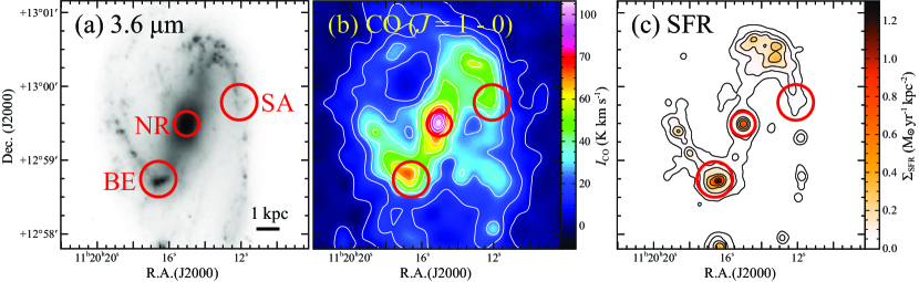
Figure 1: Observed positions (red circles) in (a) the 3.6 $\mu$m image (Kennicutt et al., 2003), (b) the integrated intensity map of CO($J=1-0$) (Kuno et al., 2007), and (c) the surface density map of the star formation rate (SFR). The contour levels are 5, 15, 25, …, 105 K km s^-1 and 0.03, 0.06, 0.12, …, 0.96 M_⊙ yr^-1 kpc^-2 for (b) and (c), respectively. The observed positions are ($\alpha$ (J2000), $\delta$ (J2000)) = (11^h 20^m 12.2^s, +12^∘ 59^′ 47.1^′′), (11^h 20^m 16.6^s, +12^∘ 58^′ 44.6^′′), and (11^h 20^m 15.5^s, +12^∘ 59^′ 29.6^′′), for NGC 3627 SA, NGC 3627 BE, and NGC 3627 NR, respectively. The sizes of the red circles, which are $29^{\prime\prime}$ and $20^{\prime\prime}$, correspond to the largest observation beam sizes of the IRAM 30 m telescope and the Nobeyama 45 m telescope, respectively. The star formation rate is derived from the H$\alpha$ and the 24 $\mu$m maps, which are observed by SINGS (Kennicutt et al., 2003), by using equation (3) (Calzetti et al., 2007). The angular resolution of H$\alpha$ is convolved to $5^{\prime\prime}$, which is the same angular resolution of 24 $\mu$m data, before the deriving SFR.

NGC 3627 is a nearby barred spiral galaxy classified as SAB(s)b in the Third Reference Catalog of Bright Galaxies (RC3: de Vaucouleurs et al., 1991) at a distance of 11 Mpc (Saha et al., 1999). Distributions of molecular gas and star-formation activities have extensively been studied by CO observations with single-dish radio telescopes (e.g., Kuno et al., 2007; Warren et al., 2010; Watanabe et al., 2011) and radio interferometers (e.g., Helfer et al., 2003; Paladino et al., 2008; Casasola et al., 2011; Beuther et al., 2017; Gallagher et al., 2018a; Law et al., 2018; Sun et al., 2018). In the present study, we observe three regions of NGC 3627: a spiral arm, a bar-end, and a nuclear region (Table 1 and Figure 1). In the bar-end region, which connects a spiral arm and a bar, intense star formation activities are identified by the H$\alpha$ emission (Smith et al., 1994; Sheth et al., 2002) and the free-free emission in the centimeter wavelength (Paladino et al., 2008; Murphy et al., 2015). Watanabe et al. (2011) reported that the star formation rate (SFR) and the star formation efficiency (SFE) are both higher in the bar-ends than in the spiral arms and the nuclear region (Table 2), where the SFRs are calculated from the H$\alpha$ and the 24 $\mu$m data (Kennicutt et al., 2003) by using a calibration method given by Calzetti et al. (2007). With a high angular resolution observation of CO($J=2-1$), Beuther et al. (2017) found two velocity components of molecular gas in the bar-end which belong to the orbital families of the spiral arm and the bar. They suggested that the high star formation activities are caused by interactions of molecular clouds at the interface between the spiral arm and the bar. On the other hand, the nuclear region of NGC 3627 shows lower star formation activities than the bar-ends (Regan et al., 2002; Watanabe et al., 2011; Murphy et al., 2015), although it is known to possess the low-ionization nuclear emission region (LINER) or low-luminous Seyfert 2 (Ho et al., 1997; Filho et al., 2000).

In this paper, we report the result of spectral line surveys toward the northern spiral arm (SA), the southern bar-end (BE), and the nuclear region (NR) of NGC 3627 (Figure 1) with the IRAM 30 m and the Nobeyama 45 m radio telescopes. By comparing the chemical composition among these three regions, we explore how chemical compositions at a scale of 1 kpc depend on galactic-scale physical environments.

2 Observations

2.1 IRAM 30 m Telescope

Observations toward SA and BE in NG 3627 were performed with the IRAM 30 m telescope at Pico Veleta in July, 2014 and December, 2014. The observed positions are shown in Figure 1 and Table 1. The beam sizes are 30–20${}^{{}^{\prime\prime}}$ and 19–17${}^{{}^{\prime\prime}}$ at the 3 mm and 2 mm band, respectively, which correspond to linear scales of 1.2–0.9 kpc and 0.8–0.7 kpc at the distance of 11.1 Mpc, respectively. The observed frequency range is from 85.0 to 116.0 GHz and from 140.0 to 148.0 GHz for SA, while it is from 85.0 to 100.5 GHz, from 108.4 to 116.0 GHz, and from 140.0 to 148.0 GHz for BE. The frequency range from 100.5 to 108.4 GHz does not involve strong spectral lines according to previous spectral line surveys toward the spiral arm of M51 (Watanabe et al., 2014). Therefore, we put a lower priority on this frequency range, and did not observe it for BE because of the limited observation time. Two EMIR (Eight MIxer Receivers) bands, E090 and E150, were used simultaneously with the dual polarization mode. The EMIR is the sideband separating receiver, which outputs the USB and LSB signals separately. The image rejection ratio is confirmed to be better than 13 dB and 10 dB for E090 and E150, respectively, according to the status report of the 30 m telescope. The system noise temperature ranged from 75 to 310 K for E090 and from 100 to 210 K for E150. Detailed frequency settings and system noise temperatures are summarized in Table 3. Backends were eight FTS (Fourier Transform Spectrometers) autocorrelators whose bandwidth and channel width are 4050 MHz and 195 kHz, respectively. The telescope pointing was checked every hour by observing the continuum source 1055+018 near the target position, and was found to be better than $\pm 5^{{}^{\prime\prime}}$. The wobbler switching mode was employed with beam throw of $\pm 120^{{}^{\prime\prime}}$ and switching frequency of 0.5 Hz. The wobbler throw is toward the azimuth direction, and hence, the absolute off-position depends on the hour angle. Nevertheless, the off-position was always out of the CO disk of NGC 3627. The intensity scale was calibrated to the antenna temperature ($T_{\rm A}^{*}$) scale by using cold and hot loads. $T_{\rm A}^{*}$ was converted to the main beam temperature $T_{\rm mb}$ by multiplying $F_{\rm eff}/B_{\rm eff}$. Here, $F_{\rm eff}$ is the forward efficiency, which is 95 % and 93 % for the 3 mm and 2 mm bands, respectively, and $B_{\rm eff}$ is the main beam efficiency, which is 81 % and 74 % for the 3 mm and 2 mm bands, respectively. Spectral baselines were subtracted for each correlator band (4050 MHz) and for each scan by fitting a 7th - 9th order polynomial to the line-free part before averaging all the scans. Then, the final spectrum for each correlator band was obtained by integrating all the scans. After the integration, the spectrum was smoothed to the frequency resolution of 5 MHz and 10 MHz for the 3 mm band and the 2 mm band, respectively (velocity resolution of $\sim 15$ km s^-1 and $\sim 20$ km s^-1, respectively).

2.2 Nobeyama 45 m Telescope

Observations toward the nuclear region of NGC 3627 (NGC 3627 NR: Figure 1 and Table 1) were performed with the Nobeyama 45 m telescope in the 3 mm band in January and March, 2015. The beam size is 20–15${}^{{}^{\prime\prime}}$, which corresponds to a linear scale of 1.2–0.9 kpc at the distance of 11.1 Mpc. The observed frequency range is from 85.0 GHz to 115.5 GHz. The TZ1H/V receiver (Nakajima et al., 2008) was used as the front end with the dual polarization mode. It is the sideband separating receiver, which outputs the USB and LSB signals separately for the two linear polarization. The image rejection ratio is assured to be better than 10 dB. The system temperature ranged from 110 to 250 K. Detailed frequency settings and system noise temperatures are summarized in Table 3. The backends were 16 SAM45 autocorrelators (Kamazaki et al., 2012) whose bandwidth and channel width each are $\sim 1600$ MHz and 0.5 MHz, respectively. The telescope pointing was checked every hour by observing the SiO maser source W-Leo, and was confirmed to be better than $\pm 6^{{}^{\prime\prime}}$. The position switching mode was employed with an off-position separated from the nuclear region by $10^{\prime}$ along the azimuthal direction. The intensity scale was calibrated to the antenna temperature ($T_{\rm A}^{*}$) scale by using the chopper-wheel method. $T_{\rm A}^{*}$ was converted to the main beam temperature $T_{\rm mb}$ by dividing $B_{\rm eff}$. Here, $B_{\rm eff}$ is the main beam efficiency, which is 41 %, 37 % and 30 % at 86 GHZ, 110 GHz, and 115 GHz, respectively. Spectral baselines were subtracted for each correlator band ($\sim 1600$ MHz) and for each scan by fitting a 6th - 9th order polynomial to the line-free part before averaging the scans. Then, the final spectra for each correlator band were obtained by integrating all the scans. After the integration, the spectrum was smoothed to the frequency resolution of 20 MHz corresponding to the velocity resolution of $\sim 60$ km s^-1 in the 3 mm band.

3 Results

3.1 Overall Spectra

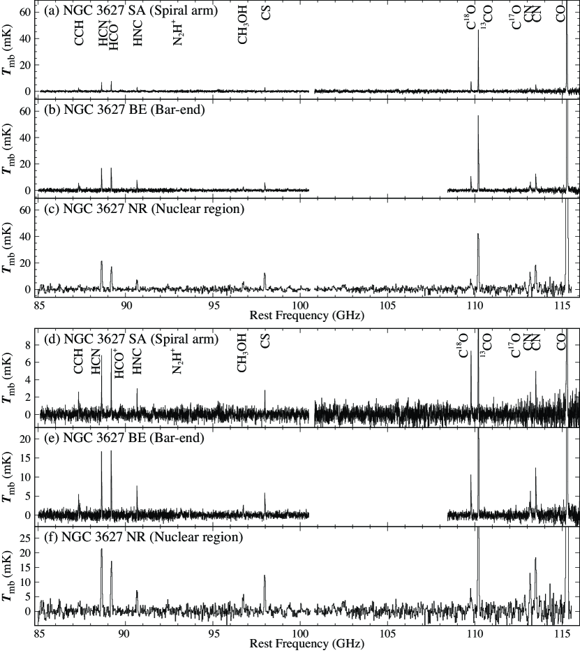
Figure 2: Composite spectra of (a) NGC 3627 SA, (b) NGC 3627 BE, and (c) NGC 3627 NR in the 3 mm band and those with magnified vertical scales of (d) NGC 3627 SA, (e) NGC 3627 BE, and (f) NGC 3627 NR. The observed positions are given in Table 1. The frequency resolution is 5 MHz, and 20 MHz, for SA and BE, and NR, respectively. The $V_{\rm LSR}$ values of 655 km s^-1, 870 km s^-1, and 715 km s^-1 are assumed for SA, BE, and NR, respectively. The emission lines contaminated from the image side band are removed.

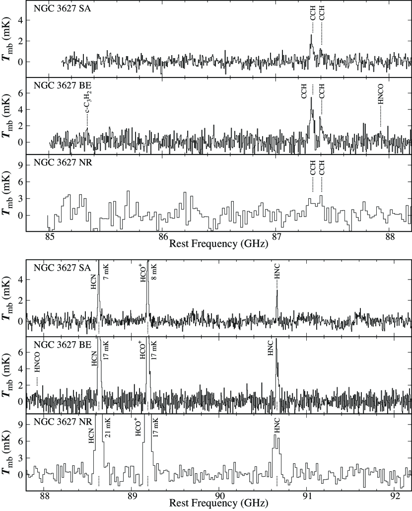
Figure 3: Spectra of NGC 3627 SA, NGC 3617 BE, and NGC 3627 NR in the 3 mm band. The spectra show the expanded version of Figure 2. The velocity resolutions and the assumed system velocities are the same as those in Figure 2. The mark ‘i-’ indicates a contamination spectrum from the image side band.

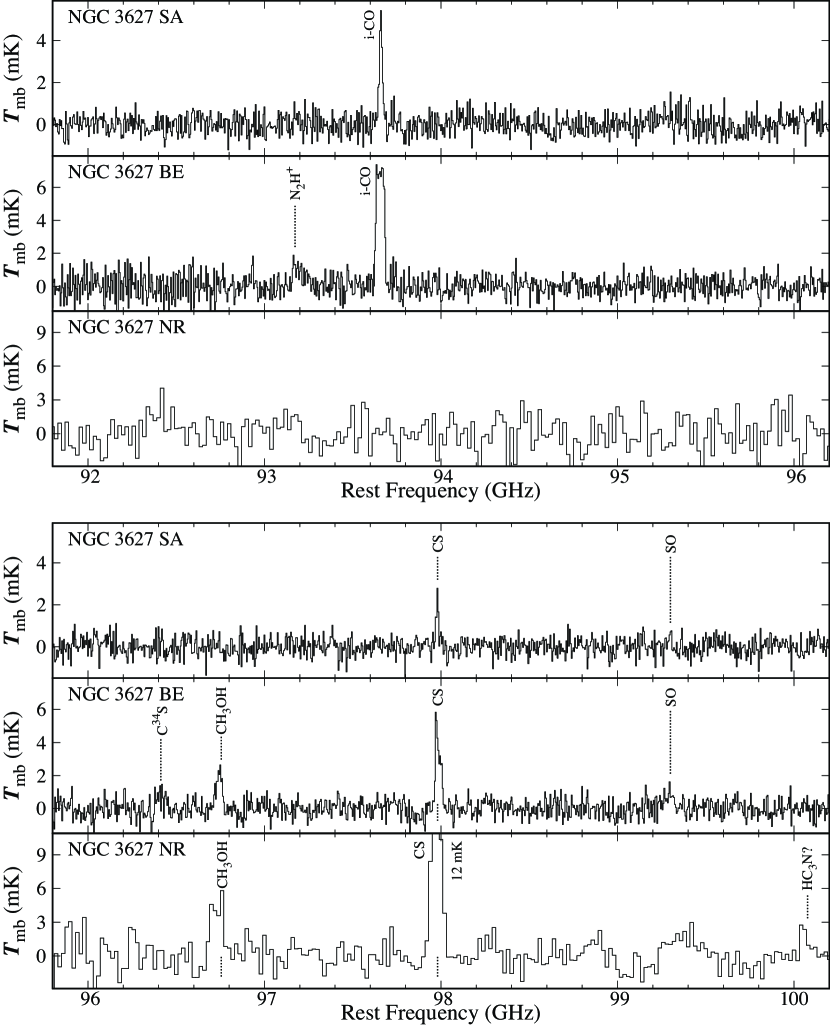
Figure 3: (Continued)

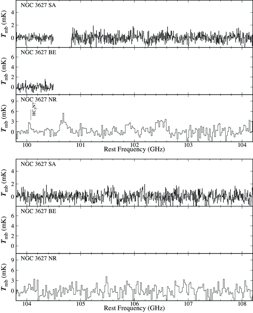
Figure 3: (Continued)

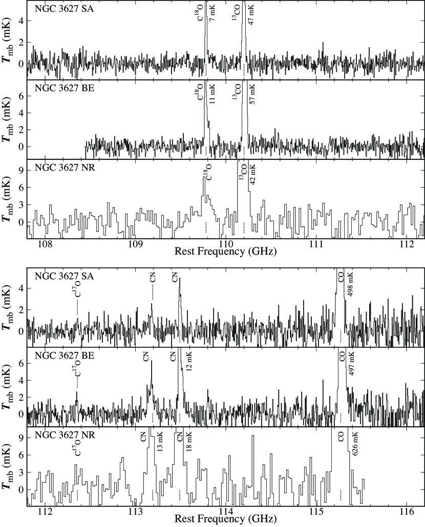
Figure 3: (Continued)

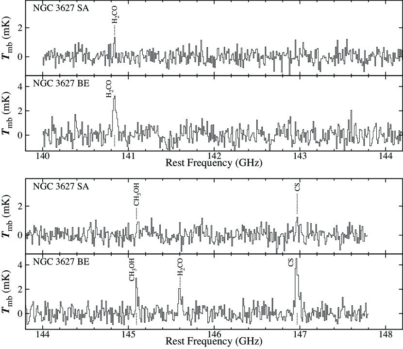
Figure 4: Spectra of (a) NGC 3627 SA and (b) NGC 3627 BE in the 2 mm band. The frequency resolution is 10 MHz. The $V_{\rm LSR}$ values of 655 km s^-1 and 870 km s^-1 are assumed for SA and BE, respectively.

Figure 2 shows the composite spectra (Figures 2a-c) and those with a magnified vertical scale (Figures 2d-f) for NGC 3627 SA, NGC3627 BE, and NGC 3627 NR in the 3 mm band. Typical rms noise levels of the 3 mm spectra are 0.4–1.3 mK, 0.5–1.6 mK, and 0.8–3.2 mK for SA, BE, and NR, respectively. Figure 3 shows the expanded version of the 3 mm spectra. In addition to the 3 mm band, the 2 mm band (140–148 GHz) was observed for SA and BE, as shown in Figure 4. Typical rms noise levels of the 2 mm spectra are 0.4 mK and 0.5–0.6 mK for SA and BE, respectively. The frequency range, the frequency resolution, and the rms noise level for the overall spectra are summarized in Table 4. A line-of-sight velocity ($V_{\rm LSR}$) of 655 km s^-1, 870 km s^-1, and 715 km s^-1 are used for SA, BE, and NR, respectively, in the spectra (Figures 2, 3, and 4). These velocities are derived from the ¹³CO($J=1-0$) mapping observation toward NGC 3627 with the Nobeyama 45 m telescope (Watanabe et al., 2011).

3.2 Identified Molecules

Tables 5, 6, and 7 summarize the parameters of emission lines detected in SA, BE, and NR, respectively. We identify molecular emission lines with the aid of the spectral line databases, Cologne Database for Molecular Spectroscopy (CDMS) maintained by University of Cologne (Müller et al., 2001; Müller et al., 2005) and Submillimeter, Millimeter and Microwave Spectral Line Catalog provided by Jet Propulsion Laboratory (Pickett et al., 1998). A criterion for the line detection is that the peak intensity and the integrated intensity exceed $3\sigma$ evaluated from the rms noise at the expected frequency of the line. If the peak intensity or the integrated intensity is less than $3\sigma$, we regarded the emission line as a marginal detection. In addition to the detected molecular lines, the upper limits to the peak intensity and the integrated intensity for important undetected lines are also given in Tables 5, 6, and 7. $V_{\rm LSR}$ and the full width at half maxima (FWHM) of each emission line are derived by Gaussian fitting, except for CCH and CN. $V_{\rm LSR}$ and FWHM are not derived for the two molecules, since the spectral lines are blended by several hyperfine structure components. Although some lines show an asymmetric profile in BE, we simply applied Gaussian fitting to the spectra. As the result, $V_{\rm LSR}$ is sometimes different from the velocity of intensity peak, and the uncertainties of $V_{\rm LSR}$ and FWHM are slightly larger than those in SA. The derived $V_{\rm LSR}$ values are almost consistent with the $V_{\rm LSR}$ values obtained by the observations of ¹³CO($J=1-0$) (Watanabe et al., 2011) in the three positions (Table 1). Moreover, we also confirm that the $V_{\rm LSR}$ values are consistent with those obtained by the other observations such as CO($J=1-0$) (Sorai et al., submitted) and CO($J=2-1$) (Leroy et al., 2009).

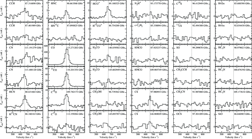
Figure 5: Line profile of each molecular transition observed in SA. Vertical dashed lines indicate $V_{\rm LSR}$ of 657 km s^-1, which is the typical systemic velocity of SA.

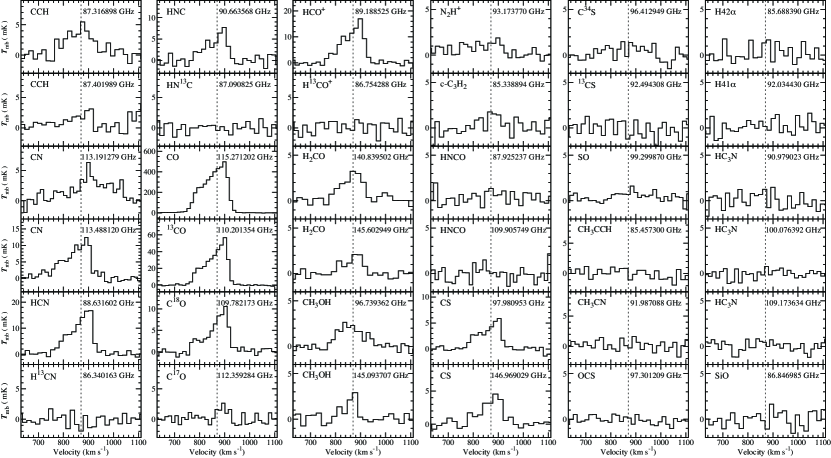
Figure 6: Line profile of each molecular transition observed in BE. Vertical dashed lines indicate $V_{\rm LSR}$ of 870 km s^-1, which is the typical systemic velocity of BE.

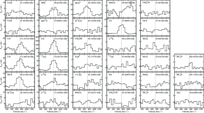
Figure 7: Line profile of each molecular transition observed in NR. Vertical dashed lines indicate $V_{\rm LSR}$ of 728 km s^-1, which is the typical systemic velocity of NR.

Figures 5, 6, and 7 display profiles of the lines listed in Tables 5, 6, and 7. In SA, 14 emission lines of 8 molecular species (CCH, CN, CO, HCN, HNC, HCO⁺, H₂CO, and CS) and two isotopologues (¹³CO and C¹⁸O) are detected in the 3 mm and 2 mm bands. In addition to these molecules, the emission line of CH₃OH is seen at 145.1 GHz with the signal-to-noise (S/N) ratio of 3 in the peak intensity and the integrated intensity. However, we do not count CH₃OH in the detected molecule, because another emission line expected at 96.74 GHz is not detected. In BE, 20 emission lines of 11 molecular species (CCH, CN, CO, HCN, HNC, HCO⁺, H₂CO, CH₃OH, N₂H⁺, CS, and SO) and 4 isotopologues (¹³CO, C¹⁸O, C¹⁸O, and C³⁴S) are detected in the 3 mm and 2 mm bands. In NR, 12 emission lines of 8 molecular species (CCH, CN, HCN, HNC, CO, HCO⁺, CH₃OH, and CS) and two isotopologues (¹³CO and C¹⁸O) are detected in the 3 mm band. Although one line of HC₃N ($J=11-10$; 100.076392 GHz) is detected with the S/N ratio of 3 and 4 in the peak intensity and the integrated intensity, respectively, no other transition lines, such as $J=10-9$ and $J=12-11$, is detected in NR. Therefore, we treat HC₃N as a marginal detection.

The undetected lines in the Table 5, 6, and 7 include the lines of the isotopologues whose normal species lines are strongly detected, such as H¹³CN, HN¹³C, H¹³CO⁺, ¹³CS, and C³⁴S. The tables also include the lines detected with relatively strong intensity in the nuclear region of other nearby galaxies such as c-C₃H₂, CH₃CCH, CH₃CN, HNCO, and OCS (e.g., Aladro et al., 2013, 2015; Lindberg et al., 2011; Martín et al., 2009; Nakajima et al., 2011, 2018). The hydrogen recombination lines of H42$\alpha$, H41$\alpha$, and H40$\alpha$ are also included as the undetected lines in Tables 5, 6, and 7.

3.3 Column Densities

Column densities of molecules are derived by assuming optically thin emission and local thermodynamic equilibrium (LTE) condition. Since only one transition line is detected for each molecule except for BE, a rotation temperature cannot be derived from the observations. We therefore adopt the three rotation temperatures, 10 K, 15 K, and 20 K, because a kinetic temperature of molecular gas is evaluated to be 10–20 K in the disk region of NGC 3627 (Law et al., 2018). A temperature of cold dust in NGC 3627 is also found to fall in this range (Galametz et al., 2012).

Before deriving the column densities, the integrated intensities are divided by the beam filling factor $\theta^{2}_{\rm source}/(\theta^{2}_{\rm source}+\theta^{2}_{\rm beam})$, where $\theta_{\rm source}$ and $\theta_{\rm beam}$ are the source size and the FWHM of the telescope beam, respectively, to compensate for frequency dependence of the beam size. Here, the source size ($\theta_{\rm source}$) is assumed to be $10^{\prime\prime}$, because distributions of HCO${}^{+}(J=1-0)$ are resolved to be $\sim 10^{\prime\prime}$ with ALMA in BE and NR(Murphy et al., 2015). We assume the same source size in SA for simplicity. The $\theta_{\rm beam}$ value is $2460/f$ arcsec and $1710/f$ arcsec for the IRAM 30 m telescope and the Nobeyama 45 m telescope, respectively, where $f$ is the observation frequency in GHz.

The column densities are evaluated by the following formula assuming the optically thin condition (e.g.: Goldsmith & Langer, 1999; Yamamoto, 2017):

$$N=\frac{3W_{\nu}k_{\rm B}U(T_{\rm rot})}{8\pi^{3}S\mu_{0}^{2}\nu}\exp\left(\frac{E_{\rm u}}{k_{\rm B}T_{\rm rot}}\right)\left\{1-\frac{\exp(h\nu/k_{\rm B}T_{\rm rot})-1}{\exp(h\nu/k_{\rm B}T_{\rm bg})-1}\right\}^{-1},$$ (1)

where $W_{\nu}$ is integrated intensity, $k_{\rm B}$ is the Boltzmann constant, $U(T)$ is the partition function, $T_{\rm rot}$ is the assumed rotation temperature, $S$ is the line strength , $\mu_{0}$ is the dipole moment, $\nu$ is the frequency, $E_{\rm u}$ is the upper state energy, $h$ is the Planck constant, and $T_{\rm bg}$ is the cosmic microwave background temperature of 2.7 K. The derived column densities are summarized in Tables 8, 9, and 10 for SA, BE, and NR, respectively. The partition function $U(T)$ is numerically calculated by the following formula:

$$U(T)=\sum_{i}g_{i}\exp\left(-\frac{E_{i}}{k_{\rm B}T}\right),$$ (2)

where $g_{i}$ and $E_{i}$ are the statical weight and the energy for the $i$-th state. The energy levels up to 300 K or more listed in CDMS are involved in the calculation. We confirm consistency between our values and those in CDMS at the temperature of 9.375 K and 18.75 K.

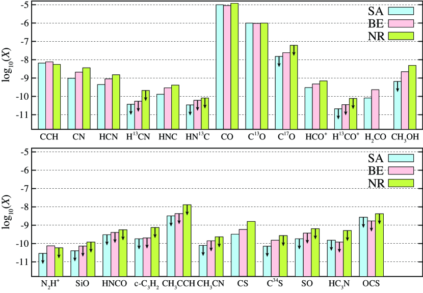
Figure 8: Fractional abundances of various molecular species relative to H₂ in NGC 3627 SA (blue), NGC 3627 BE (pink), and NGC 3627 NR (green). The fractional abundances are calculated by assuming the rotation temperature of 10 K for all the positions. Down arrows indicate upper limits.

In addition to the column densities, the fractional abundances relative to the molecular hydrogen (H₂) are evaluated. For this purpose, the column densities of H₂ are derived from the column densities of C¹⁸O by assuming the [C¹⁸O]/[H₂] ratio of $1.7\times 10^{-7}$ (Frerking et al., 1982; Goldsmith et al., 1997). Here, we assume that the [C¹⁸O]/[H₂] ratio in NGC 3627 is the same as that in our Galaxy, because the elemental abundance in NGC 3627 is also similar to that in our Galaxy (Contini, 2017). The derived fractional abundances are also summarized in Tables 8, 9, and 10 for SA, BE, and NR, respectively. Figure 8 shows histograms of the fractional abundances derived at $T_{\rm rot}$ = 10 K for the three positions.

Variations of the fractional abundances by changing the assumed rotation temperature from 10 K to 20 K are smaller than those of the column densities for most molecules. This is because the temperature effects are mostly compensated by taking the ratio of the two column densities. In fact, variations of the fractional abundances are less than 10 % except for CH₃OH, c-C₃H₂, CH₃CCH, HC₃N, and OCS, while those of the column densities are $10-30$ %. Although variation of the fractional abundances is slightly higher for CH₃OH, c-C₃H₂, and CH₃CCH, it is evaluated to be $\sim 20$ % or less. On the other hand, the fractional abundances of HC₃N and OCS show larger variation by a factor of two, because their column densities are derived by using the lines with relatively high upper state energies of $\sim 20$ K. As shown in Equation 1, the column densities are proportional to $\exp(E_{\rm u}/k_{\rm B}T_{\rm rot})$, and hence, the column densities are sensitive to the assumed rotation temperature for the lines with $E_{\rm u}/k_{\rm B}>T_{\rm tot}$. However, this effect does not cause a serious impact on the following discussion, because only upper limits are derived for HC₃N and OCS. In the following sections, we will use the fractional abundances relative to H₂ or C¹⁸O to compare chemical compositions in different sources.

3.4 SFR and SFE

The SFR (Figure 1c) is calculated by using the H$\alpha$ and Spitzer 24 $\mu$m data (Kennicutt et al., 2003). Before the calculation, H$\alpha$ image is convolved by a Gaussian kernel to be the angular resolution of $5^{\prime\prime}$ corresponding to the angular resolution of the 24 $\mu$m data. The calibration of SFR is done by the following equation (Calzetti et al., 2007):

$${\rm SFR}=5.3\times 10^{-42}[L({\rm H\alpha})_{\rm obs}+0.031\times L({\rm 24\mu m})]\,({\rm M_{\odot}yr^{-1}}),$$ (3)

where $L({\rm H\alpha})$ and $L({\rm 24\mu m})$ are luminosities of the H$\alpha$ and 24 $\mu$m emission, respectively, in erg s^-1. The surface density of SFR ($\Sigma_{\rm SFR}$) is evaluated within the observation beam of $22^{\prime\prime}$, $22^{\prime\prime}$, and $16^{\prime\prime}$ for SA, BE, and NR, respectively. The surface density of molecular gas mass $\Sigma_{\rm gas}$ is calculated from the column density of H₂ derived from the C¹⁸O data assuming the rotation temperature of 10 K. The contribution of He is involved in $\Sigma_{\rm gas}$ by multiplying a factor of 1.36. Here, the source size of $10^{\prime\prime}$ is not taken into account for both $\Sigma_{\rm SFR}$ and $\Sigma_{\rm gas}$. The SFE is calculated as $\Sigma_{\rm SFR}/\Sigma_{\rm gas}$. The $\Sigma_{\rm SFR}$, $\Sigma_{\rm gas}$, and SFE values are summarized in Table 2.

3.5 Integrated Intensity Ratios of CO Isotopologues

We calculate integrated intensity ratios of the CO isotopologues in the three positions. The ¹²CO($J=1-0$)/¹³CO($J=1-0$) intensity ratios are $11.9\pm 0.3$, $10.8\pm 0.2$, and $14\pm 1$ in SA, BE, and NR, respectively. These values are consistent with the intensity ratios in NGC 3627 previously observed with the Nobeyama 45 m telescope (Watanabe et al., 2011) and the IRAM 30 m telescope (Cormier et al., 2018). Law et al. (2018) reported the ¹²CO($J=2-1$)/¹³CO($J=2-1$) ratios to be $\sim 4$ and $2.5\pm 0.2$ in BE and NR, respectively, from the SMA observation at a resolution of $2.33^{\prime\prime}\times 1.85^{\prime\prime}$. Although the ratios are for the $J=2-1$ transition, these values are much lower than our values. As discussed in Law et al. (2018), ¹²CO can trace much more diffuse molecular gas than that of ¹³CO and be detectable everywhere. As the result, the ratios obtained with a larger beam size tend to be larger.

However, this trend does not always work for any case. For instance, Tan et al. (2011) observed the ¹²CO($J=1-0$)/¹³CO($J=1-0$) ratio with the PMO 14 m telescope toward various positions in NGC 3627. Although their ratio is consistent with our value in NR, their value of $5.3\pm 1.3$ at the position covering BE is significantly lower than our value of $10.8\pm 0.2$ at BE in spite of a larger observation beam ($60^{\prime\prime}$). This implies the ¹²CO/¹³CO ratio is sensitive to the physical properties and the distributions of molecular cloud involved in the beam.

The ¹³CO($J=1-0$)/C¹⁸O($J=1-0$) intensity ratios observed in the present study are $6\pm 1$, $5.4\pm 0.6$, and $6\pm 3$ in SA, BE, and NR, respectively. The ratio for NR is similar to the mean intensity ratio of $6.0\pm 0.9$ for the nuclear regions of nearby galaxies (Jiménez-Donaire et al., 2017). On the other hand, the ratios in SA and BE are found to be lower than the mean intensity ratio of $9.0\pm 1.1$ in the disk region of NGC 3627 (Jiménez-Donaire et al., 2017).

The lower ratios in SA and BE would originate from the optical depth effect. If the optical depth of ¹³CO is higher in SA and BE than in the other disk regions, the ratio would be lower in SA and BE. In our observation, the optical depth of the ¹³CO line are evaluated to be 0.018 for both SA and BE with the temperature of 15 K and the assumed source size of $10^{\prime\prime}$. However, the optical depth of the ¹³CO line is likely higher than the above value, because distribution of molecular gas is expected to be clumpy. In addition to the high angular resolution observation of ¹²CO in NGC 3627 with the radio interferometers (Gallagher et al., 2018a, b; Law et al., 2018; Sun et al., 2018), observations of the CO isotopologues have recently been conducted with the ALMA at a scale of $1^{\prime\prime}$ (Gallagher et al., 2018a). The result will be useful for examining the possibility of the clumpy structure in future.

Another possibility would be different ¹⁸O abundances for the different positions. Jiménez-Donaire et al. (2017) reported that the intensity ratios are lower in the vicinity of active star forming regions than quiescent regions among the nearby galaxies. They claimed that the trend can be explained, for instance, by enhancement of the ¹⁸O abundance by nucleosynthesis in the massive stars. Since the SFR is relatively higher in SA and BE than the other disk regions in NGC 3627 (Table 2 and Watanabe et al. (2011)), the active star formation might result in the lower ¹³CO($J=1-0$)/C¹⁸O($J=1-0$) intensity ratios in SA and BE in principle. However, it is not obvious whether such an effect could cause the observable effect on the ratios. Note that, for this reason, we employ the standard [C¹⁸O]/[H₂] ratio to derive the H₂ column density, as mentioned in Section 3.3.

4 Discussion

In this observation, we have systematically revealed chemical compositions in the spiral arm (SA), the bar-end (BE), and the nuclear region (NR) of NGC 3627 by the spectral line survey. We here compare the fractional abundances among these three regions and discuss them in terms of physical environments and evolutionary stages in the following subsections. In addition, we also compare the chemical composition in NGC 3627 BE with those in the spiral arm of nearby galaxy M51 and the molecular cloud W51 in our Galaxy. Then, we compare the chemical composition in NR of NGC 3627 with that in the nuclear region of NGC 1068 to study effects of nuclear activities on the chemical composition.

4.1 Comparisons of Chemical Compositions between SA and BE

Figure 9a shows a correlation plot of the fractional abundances between SA and BE which are derived under the assumption of the rotation temperature of 10 K. Although the SFE is higher in BE than in SA by a factor of 5 (Table 2), the chemical composition is similar to each other. In fact, the Pearson correlation coefficient is found to be 0.999. Here, we do not take into account of the uncertainties in the calculation. In addition, we exclude the upper limit values from the correlation-coefficient calculations. The correlation coefficient changes by 0.001, even if the correlation coefficients are calculated from the fractional abundances assuming different rotation temperatures. Because of the high SFE in BE, star formation feedbacks such as UV radiation from high-mass stars and shocks by outflows from protostars are expected to be prominent in BE, which would consequently affect the chemical composition in BE in comparison with those in SA. However, no significant effect of such star formation feedbacks can be recognized in the chemical composition observed at a scale of $\sim 1$ kpc. The feedback effects would be diluted by the large observation beam, while the chemical composition of extended molecular gas makes a dominant contribution to the spectrum. Similar results have been reported in observations of nearby galaxies and Galactic molecular clouds (e.g., Nishimura et al., 2016a, 2017; Watanabe et al., 2014, 2017).

On the other hand, most of the fractional abundances are found to be systematically higher in BE than SA by a factors of 2-3, except for CCH and ¹³CO. The difference cannot be explained by the assumed beam filling factors. Even if we assume a smaller source size of $1^{\prime\prime}$ instead of $10^{\prime\prime}$, the fractional abundances become higher by only a factor of 1.1. Therefore, the higher fractional abundances indicate that there is more dense molecular gas in BE than SA, because these molecular transition lines likely trace denser molecular gas than the gas traced by CO isotopologues due to their higher critical densities (e.g. Nishimura et al., 2017).

However, the relation of the higher fraction of dense gas to higher SFE in BE is not straightforward, because the relation itself is still controversial. Muraoka et al. (2016) reported that volume density of H₂ ($n_{\rm H_{2}}$) is correlated with SFE in their observation of the nearby galaxy NGC 2903 with the Nobeyama 45 m telescope. Since high $n_{\rm H_{2}}$ is expected in the region with the high dense gas fraction, the high dense gas fraction is a possible origin of the high SFE. On the other hand, Law et al. (2018) found no correlation between the $n_{\rm H_{2}}$ and SFE in NGC 3627 at a scale of kpc. In addition, Usero et al. (2015) also reported that no correlation can be seen between SFE and dense gas fraction evaluated from CO(1-0) and HCN(1-0) observed with IRAM 30 m telescope in nearby galaxies. Therefore, we need more investigations on the relation in NGC 3627.

While the critical density of CCH is higher than those of CO isotopologues, the fractional abundance in SA is similar to that in BE. This would be a result of the wider spatial distribution of CCH than those of the other molecules except for CO and its isotopologues. In fact, the extended CCH distributions are found in the Galactic molecular clouds (e.g., Nishimura et al., 2017; Pety et al., 2017). Nishimura et al. (2017) conducted a wide-field mapping observation of the Galactic molecular cloud W3(OH), and found that the CCH/HCO⁺ ratio is higher in the outer regions of molecular clouds than the central parts. According to Nishimura et al. (2017), the abundance of CCH is high in the periphery of a molecular cloud where the UV photon can penetrate, because CCH is efficiently produced from C⁺ ionized by the interstellar UV field. Another reason would be the excitation conditions necessary for producing the CCH emission. Because the dipole moment of CCH (0.77 Debye) is smaller than those of other molecules such as HCN (2.99 Debye) and CS (1.96 Debye), the critical density of CCH is lower than these molecules (e.g. Nishimura et al., 2017). Therefore, CCH can trace more diffuse gas than the other molecules due to chemical and physical reasons.

4.2 Comparison with a Spiral Arm of M51 and a Galactic Molecular Cloud W51

Here, we compare the chemical composition in NGC 3627 BE with those in a spiral arm in M51 and a giant molecular cloud W51 in our Galaxy. Since these sources are molecular clouds located in a disk region of galaxies, their chemical compositions are free from the effect of nuclear activities such as AGNs and starbursts. The chemical composition in SA is similar to that in BE, and hence, we focus only on BE in this section.

M51 is a nearby face-on spiral galaxy ($d=8.4$ Mpc Feldmeier et al., 1997; Vinkó et al., 2012). The elemental abundance in M51 (N/O:$\sim 0.25$, S/O:$0.03$: Bresolin et al., 2004) is similar to that in NGC 3627 (N/O:$\sim 0.23$, S/O:$\sim 0.025$: Contini, 2017). Figure 9b is a correlation plot of the molecular abundances between BE and M51 P1 (Watanabe et al., 2014). The rotation temperature assumed for BE is 10 K, and that for M51 P1 is 5 K. The plot shows a good correlation with a correlation coefficient of 0.989. The fractional abundances in BE are thus similar to those in M51 P1 for most of the species. Because the beam size of the observation ($\sim 25^{\prime\prime}$) corresponds to $\sim 1$ kpc at the distance of M51, the spatial scale of the M51 observation is similar to that of our observation toward NGC 3627. It is reported that the SFE is lower in M51 P1 ($5.9\times 10^{-10}$ yr^-1) than in BE ($5.7\times 10^{-9}$ yr^-1) by a factor of 10 (Watanabe et al., 2014). In spite of the different SFE, the chemical compositions in BE and M51 P1 are similar to each other. Therefore, the chemical compositions of molecular gas at a scale of $\sim 1$ kpc are thought to be unaffected by the star-formation activities.

Figure 9c shows a correlation plot between BE and the Galactic molecular cloud W51 (Watanabe et al., 2017). The rotation temperature assumed for BE is 10 K. W51 is the molecular cloud complex with the vigorous massive star forming regions. The fractional abundances in W51 were obtained from the spectrum stacked over the $39\,{\rm pc}\times 47\,{\rm pc}$ area centered at the W51A molecular cloud mapped with the Mopra 22 m telescope. Therefore, the fractional abundances in W51 represent those at the scale of a molecular cloud. The elemental abundance in the Galaxy is also similar to that in NGC 3627 (Contini, 2017). A strong positive correlation (0.989) seen in Figure 9c indicates that the chemical composition in BE is also similar to the molecular-cloud-scale ($\sim 50$ pc) chemical composition in the spiral arm of our Galaxy.

4.3 Nuclear Region of NGC 3627

Figures 9d and 9e are correlation plots of the fractional abundances between SA and NR, and between BE and NR, where the rotation temperature of 10 K is assumed. Although the fractional abundances are higher in NR than SA and BE by factors of $\sim 5$ and $\sim 2$, respectively, the correlation coefficients are as high as 0.991–0.993 for the both plots. The strong positive correlation suggests that the chemical compositions are similar to each other between BE and NR, although NR possesses a LINER/Seyfert 2 nucleus (Ho et al., 1997; Filho et al., 2000). The X-ray luminosity in the 2-10 keV band is reported to be $3.2\times 10^{39}$ erg s^-1, which is lower than that of prototypical Seyfert nuclei in NGC 1068 by three orders of magnitude (Brightman & Nandra, 2011). Therefore, the effect of nuclear activities would be limited to very small region ($<100$ pc), and would not significantly affect the chemical composition in the major part of molecular gas in the beam.

In spite of the overall similarity, we can see small differences between SA and NR and between BE and NR. For example, the fractional abundances are higher in NR than SA and BE, except for CCH and N₂H⁺. The trend of higher fractional abundances in NR is not artificially caused by the assumption of the low rotation temperature of 10 K, although higher rotation temperatures were reported in the nuclear region of other galaxies at a scale of $\sim 1$ kpc (e.g. Aladro et al., 2011, 2013; Nakajima et al., 2018). As seen in Table 10, the fractional abundances derived by assuming the temperature of 20 K are similar to or slightly higher than those derived by assuming the temperature of 10 K. The similar trend can be reproduced by assuming higher temperature (e.g. 100 K), except for HC₃N. Therefore, even if the rotation temperature in NR is higher than 10 K due to the nuclear activity, we will see the same trend of higher fractional abundances in NR. The higher fractional abundances would be a result of a higher fraction of the denser molecular gas in NR than in the other positions. On the other hand, the abundances of CCH are similar among the three regions (Figure 9d and 9e). As discussed in Section 4.1, CCH traces widely extended molecular gas as CO and its isotopologues rather than dense gas traced by other molecules. Hence, the trend of CCH in Figures 9d and 9e seems reasonable.

The N₂H⁺ abundance in NR is found to be similar to or lower than that in BE (Figure 9e). This result indicates inefficient production of N₂H⁺ and/or efficient destruction working in NR. There are two major destruction processes for N₂H⁺; the reaction with CO and the dissociative recombination with an electron. However the destruction by CO would not be the cause of the different N₂H⁺ abundances, because the fractional abundances of various molecules, for which H₂ column density is evaluated from C¹⁸O, are higher in NR than in SA and BE. If the CO fractional abundance were enhanced in NR, the fractional abundances of the other molecules would be calculated to be lower in NR than in SA and BE. Moreover, the dissociative recombination would not be the case, either. Because the SFE is derived to be higher in BE than in NR, the UV radiation field is expected to be higher in BE than NR. The electron abundance is consequently expected to be higher in BE than NR, which contradicts with the lower N₂H⁺ abundance in NR. However, the electron abundance could be enhanced by strong X-ray radiation in NR due to nuclear activities, which may contribute to destruction of N₂H⁺ in NR.

Pety et al. (2017) reported that N₂H⁺ traces the densest regions of Orion B cloud, while HCN and HCO⁺ traces the less dense molecular gas with H₂ density of $\sim 1500$ cm^-3. They discussed that N₂H⁺ can only survive in cold and dense gas where CO is frozen on the dust grain. Kauffmann et al. (2017) also reported that N₂H⁺(1-0) traces the dense gas at a characteristic H₂ density of $\sim 4000$ cm^-3, while HCN(1-0) can trace rather diffuse gas at the H₂ density of $\sim 870$ cm^-3, on the basis of the observations of the Orion molecular cloud. If this picture is applied to the present case, a fraction of ‘cold dense gas’ is lower in NR than in BE. In any case, the lower abundance of N₂H⁺ in NR seems to suggest some important physical conditions. Interferometric studies revealing the distributions of N₂H⁺ and other molecules are awaited for further discussions.

4.4 Comparisons of the Nuclear Region with NGC 1068

Here, we compare the chemical composition of NR with that of Seyfert 2 type AGN NGC 1068, because NGC 3627 possesses LINER or low-luminous Seyfert 2 AGN (Ho et al., 1997; Filho et al., 2000). The AGNs are thought to be powered by accretion of material to the super-massive black hole at the center of galaxy and to emit strong X-ray. As the result, the chemical compositions of molecular gas around the AGNs are expected to be affected by it (X-ray dominated region) (e.g., Lepp & Dalgarno, 1996; Maloney et al., 1996; Meijerink & Spaans, 2005; Meijerink et al., 2007). The AGN activity is thought to be higher in NGC 1068 than in NGC 3627, because the intrinsic luminosity of X-ray in the 2-10 keV band is reported to be higher in NGC 1068 ($1.6\times 10^{42}$ erg s^-1) than in NGC 3627 ($3.2\times 10^{39}$ erg s^-1) by three orders of magnitude (Brightman & Nandra, 2011).

Figure 9f shows a correlation plot of fractional abundances relative to C¹⁸O between NR and the nuclear region of NGC 1068 (Aladro et al., 2013, 2015). Here, the rotation temperature assumed for NR is 10 K. Aladro et al. (2015) derived column densities of molecules in NGC 1068 using the spectral line survey data observed with the IRAM 30 m telescope by assuming the rotation temperature of 10 K. The fractional abundances of NGC 1068 are therefore the ones averaged over $\sim 1.5$ kpc. The correlation coefficient of the plot is as high as 0.84. Although it is slightly lower than those among the disk regions in nearby galaxies and our Galaxy (W51), it indicates that the chemical compositions are similar to each other despite different X-ray luminosities. The similarity implies that the effect of X-ray is diluted by an overwhelming contribution of ambient molecular clouds due to the large observation beam ($\sim 1$ kpc).

The fractional abundances are generally found to be higher in NGC 1068 than NGC 3627 NR by a factor of two except for CH₃OH, HC₃N, and CS, although the chemical composition are almost similar to each other as a whole. The higher abundances would indicate a higher fraction of dense molecular gas in NGC 1068 than NGC 3627 NR. On the other hand, the abundances of CH₃OH, CS, and HC₃N are higher in NGC 3627 NR than NGC 1068 by a factor of two, although HC₃N is tentative detection. It is reported that CH₃OH and CS are enhanced by liberation from ice mantle of dust grains due to shocks in the Galactic sources, for instance, outflow shocks (e.g., Bachiller & Pérez Gutiérrez, 1997). In external galaxies, the enhancement of CH₃OH is reported in the bar region, where shocks due to cloud-cloud collisions are expected (Meier & Turner, 2005). It has also been seen in shocked regions caused by interactions of molecular gas in merging galaxies (Saito et al., 2017; Ueda et al., 2017). However, no sign of shocks such as outflows from the nuclear region and active star formation is reported for NGC 3627 NR even by high angular resolution observations with interferometers (Casasola et al., 2011; Murphy et al., 2015; Law et al., 2018). Therefore, the shock would not be the case for the enhancement, although there may exist accretion shocks in the nuclear region of NGC 3627 in principle. As for another possibility, one may think that these molecules could more efficiently be destroyed in NGC 1068 by strong radiation from the AGN. However, CS, CH₃OH, and HC₃N are found to be associated with the circumnuclear disk in NGC 1068 by the ALMA observation (Takano et al., 2014). Thus, the destruction by the radiation would not explain the differences, either. An investigation of overabundant CH₃OH and CS in NGC 3627 will be an interesting future problem.

4.5 Chemical Compositions of Molecular Clouds

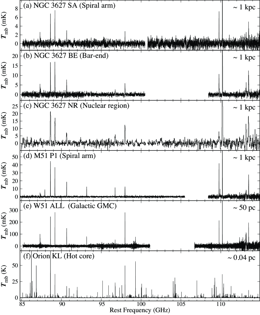
Figure 10: Spectra of (a) NGC 3627 SA, (b) NGC 3627 BE, (c) NGC 3627 NR, (d) M 51 P1 (Watanabe et al., 2014), (e) W51 (Watanabe et al., 2017), and (f) Orion KL (Watanabe et al., 2015) in the 3 mm band. The beam sizes of the observations in the linear scale are shown in the right side of panels.

The chemical compositions of molecular clouds at a scale from 1 kpc to 10 pc have been studied for NGC 3627 and M51 (Watanabe et al., 2014, 2016), as well as the Galactic molecular clouds W51 (Watanabe et al., 2017) and W3 (Nishimura et al., 2017). All these sources have the similar elemental abundances. From these studies, we find that the chemical composition of molecular gas is similar among different galaxies and among different regions with different star-formation/nuclear activities, when we observe them in the 3 mm band at a scale larger than a molecular cloud ($>10$ pc). Figures 10a-e show the spectra observed in NGC 3627 SA, BE, NR, M51 P1, and W51 in the 3 mm bands. Indeed, the relative intensities of molecular lines look similar among the five sources.

On the other hand, the spectrum of the hot core (Orion KL: Figure 9f) observed at a scale of 0.04 pc is much different from the other spectra. The difference reflects a different chemical composition in the hot core from those in molecular clouds as well as the different excitation condition; namely hotter and denser gas in the hot core than in molecular clouds. At a scale of a molecular cloud core ($\sim 0.01$ pc), the chemical composition is largely controlled by its evolutionary state (e.g. Suzuki et al., 1992) and ambient UV environments (e.g., Tielens & Hollenbach, 1985). Therefore, we can make use of the chemical composition as tracers of their evolutionary stages and physical environments in the Galactic objects. However, such chemical features of molecular cloud cores are smeared out, when we observe them at a scale larger than the molecular clouds. The sound crossing time scale of the molecular clouds ($>10^{7}$ years), which is estimated by assuming a typical size of 10 pc (e.g.: Roman-Duval et al., 2010) and a sound speed of 0.3 km s^-1, is longer than the time scale of chemical equilibrium ($\sim 10^{5-6}$ years). Here, the sound speed $c_{\rm s}$ is calculated by the following formula:

$$c_{\rm s}=\sqrt{\gamma\frac{k_{\rm B}}{\mu m_{\rm H}}T},$$ (4)

where $\gamma$ is the specific heat ratio of gas (5/3), $\mu$ is the molecular mass, and $m_{\rm H}$ is the hydrogen mass. We evaluated the sound speed with $\mu=2$ and $T=10$ K. Therefore, the chemical composition in the molecular clouds is thought to be close to that in the chemical equilibrium state, which is almost independent of evolutionary history of molecular clouds.

However, Harada et al. (2019) recently reported that the chemical compositions of the molecular clouds can be reproduced by their time-dependent chemical model with a relatively short time of $\sim 10^{5}$ years. Because this time scale is much shorter than the lifetime of molecular cloud and the time scale for chemical equilibrium, they suggested that a turbulence in the molecular clouds regulates the chemical clock. Namely, the chemical composition is refreshed by the interstellar UV radiation when the turbulence brings the molecular gas from the inside to the surface of the molecular cloud where the visual extinction is low.

In spite of the similarity of the chemical composition at a scale of molecular clouds, a different chemical composition has been found in metal poor galaxies (Nishimura et al., 2016a, b), shocked regions of merging galaxies (e.g. Saito et al., 2017; Ueda et al., 2017), and nuclear regions of galaxies observed at a scale of a few hundred pc (e.g., Costagliola et al., 2015; Meier et al., 2015; Ando et al., 2017). In these objects, the chemical compositions are thought to reflect low elemental abundances, gas dynamics at molecular cloud scales, and extreme environments due to feedback from nuclear activity and vigorous star-formation. To highlight chemical characteristics in these objects, the result of this study can be used as a ‘standard’ template of chemical composition without such influences.

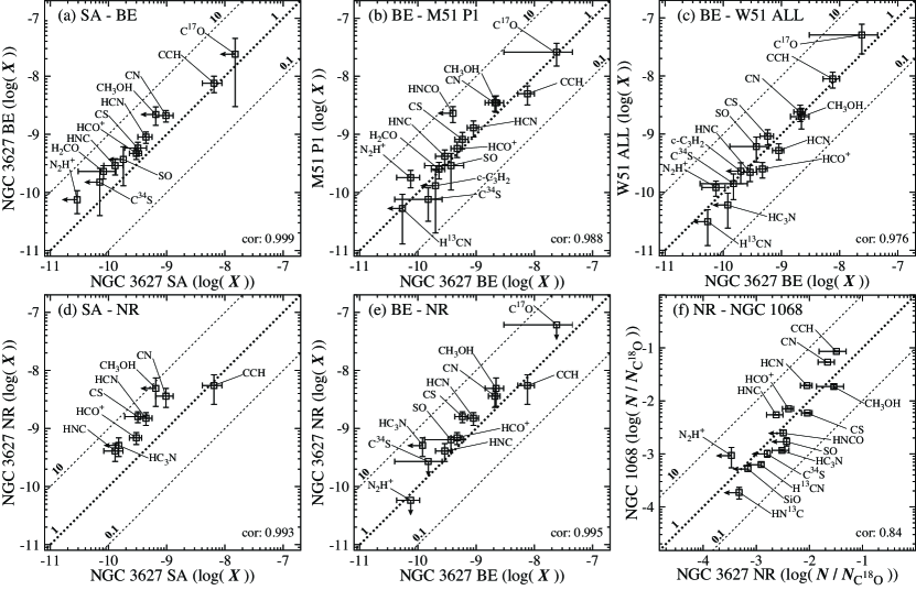
Figure 9: Correlation plots of fractional abundances relative to H₂ ($X$) (a) between NGC 3627 SA and NGC 3627 BE, (b) between NGC 3627 BE and M51 P1, (c) between NGC 3627 BE and W51, (d) between NGC 3627 SA and NGC 3627 NR, and (e) between NGC 3627 BE and NGC 3627 NR. (f) Correlation plot of the fractional abundances relative to C¹⁸O between NGC 3627 NR and NGC 1068. The fractional abundances are calculated by assuming the rotation temperature of 10 K for all the positions of NGC 3627. The rotation temperature is assumed to be 5 K for M51 P1 (Watanabe et al., 2014). Dashed lines indicate the fractional abundance ratios of 0.1, 1, and 10. Arrows indicate the upper limits to the fractional abundances. The Pearson correlation coefficient (cor.) between $\log(X_{i,{\rm A}})$ and $\log(X_{i,{\rm B}})$ is shown in the bottom-right corner. The upper limit values are excluded from the calculation of the correlation coefficients.

Table 1: Observation Positions

Position	R.A. (J2000)	Dec. (J2000)	$V_{\rm sys}$ (km s-1)a
Spiral Arm (SA)	11h 20m 12.1s	+12∘ 59′ 47.1′′	655
Bar-End (BE)	11h 20m 16.6s	+12∘ 58′ 44.6′′	870
Nuclear Region (NR)	11h 20m 15.3s	+12∘ 59′ 29.6′′	715

Table 2: Surface Density of Molecular Gas, and Star Formation Rate, and Star Formation Efficiency

Position	$\Sigma_{\rm SFR}$ (M${}_{\odot}\,{\rm yr^{-1}}\,{\rm kpc^{-2}}$)	$\Sigma_{\rm gas}$ (M${}_{\odot}\,{\rm kpc^{-2}}$)	SFE (yr-1)
Spiral Arm (SA) a	$0.035\pm 0.007$	$(2.7\pm 0.7)\times 10^{7}$	$(1.3\pm 0.4)\times 10^{-9}$
Bar-End (BE) a	$0.31\pm 0.06$	$(5.5\pm 1.3)\times 10^{7}$	$(5.7\pm 1.7)\times 10^{-9}$
Nuclear Region (NR)b	$0.20\pm 0.04$	$(1.1\pm 0.6)\times 10^{8}$	$(1.8\pm 1.0)\times 10^{-9}$

Table 3: Observation Settings

Spiral Arm (SA)
	Telescope	Receiver	LSB (GHz)	USB (GHz)	$T_{\rm sys}$ (K) a
Set 1	IRAM 30 m	E090	85.1 – 92.9	100.8 – 108.6	60 – 140
Set 2	IRAM 30 m	E090	85.1 – 92.9	N/A	70 – 110
		E150	140.0 – 147.8	N/A	80 – 140
Set 3	IRAM 30 m	E090	92.7 – 100.5	108.4 – 116.2	60 – 190
Bar-End (BE)
	Telescope	Receiver	LSB (GHz)	USB (GHz)	$T_{\rm sys}$ (K) a
Set 1	IRAM 30 m	E090	85.0 – 92.8	N/A	80 – 110
		E150	140.0 – 147.8	N/A	90 – 150
Set 2	IRAM 30 m	E090	92.7 – 100.5	108.4 – 116.2	70 – 290
Nuclear Region (NR)
	Telescope	Receiver	LSB (GHz)	USB (GHz)	$T_{\rm sys}$ (K) a
Set 1	Nobeyama 45 m	TZ1H/V	85.0 – 88.1	97.0 – 100.3	140 – 250
Set 2	Nobeyama 45 m	TZ1H/V	88.0 – 91.1	99.8 – 103.1	110 – 180
Set 3	Nobeyama 45 m	TZ1H/V	91.0 – 94.1	103.0 – 106.1	110 – 260
Set 4	Nobeyama 45 m	TZ1H/V	94.0 – 97.1	106.0 – 109.1	140 – 250
Set 5	Nobeyama 45 m	TZ1H/V	97.0 – 100.3	109.0 – 112.1	130 – 160
Set 6	Nobeyama 45 m	TZ1H/V	99.8 – 103.1	112.1 – 115.5	150 – 210

Table 4: Summary of Spectra

Position	Band	Frequency	Resolution	Sensitivity
		(GHz)	(MHz)	(mK)
NGC 3627 SA	3 mm	85.1 – 100.5, 100.8 – 116.2	5	0.4 – 1.3
	2 mm	140.0 – 147.8	10	0.4
NGC 3627 BE	3 mm	85.1 – 100.5, 108.4 – 116.2	5	0.5 – 1.6
	2 mm	140.0 – 147.8	10	0.5 – 0.6
NGC 3627 NR	3 mm	85.0 – 115.5	20	0.8 – 3.2

Table 5: Line Parameters in NGC 3627 SA

	Transition	Freq.	$E_{\rm u}$	S$\mu^{2}$	$T_{\rm mb}$ Peak	$\int T_{\rm mb}dv$	$V_{\rm LSR}$	FWHM
		(GHz)	(K)		(K)	(K km s-1)	(km s-1)	(km s-1)
c-C3H2	$2_{1\,2}-1_{0\,1}$	85.338894	4.1	16.1	$<0.001$	$<0.04$	$\cdots$	$\cdots$
CH3CCH	$5_{0}-4_{0}$	85.457300	12.3	6.15	$<0.001$	$<0.04$	$\cdots$	$\cdots$
H42$\alpha$		85.688390			$<0.001$	$<0.04$	$\cdots$	$\cdots$
H13CN	$1-0$	86.340163	4.1	8.91	$<0.001$	$<0.03$	$\cdots$	$\cdots$
H13CO+	$1-0$	86.754288	4.2	15.2	$<0.001$	$<0.03$	$\cdots$	$\cdots$
SiO	$2-1$	86.846985	6.3	19.2	$<0.001$	$<0.03$	$\cdots$	$\cdots$
HN13C	$1-0$	87.090825	4.2	9.30	$<0.001$	$<0.03$	$\cdots$	$\cdots$
CCH	$N=1-0,J=3/2-1/2,F=2-1$	87.316898	4.2	0.988	0.003 (1)	0.23 (7)		$\cdots$
CCH	$N=1-0,J=3/2-1/2,F=1-0$	87.328585	4.2	0.492			$\cdots$	$\cdots$
CCH	$N=1-0,J=1/2-1/2,F=1-1$	87.401989	4.2	0.492	0.001 (1)	0.10 (6)		$\cdots$
CCH	$N=1-0,J=1/2-1/2,F=0-1$	87.407165	4.2	0.198			$\cdots$	$\cdots$
HNCO	$4_{0\,4}-3_{0\,3}$	87.925237	10.5	9.99	$<0.001$	$<0.04$	$\cdots$	$\cdots$
HCN	$1-0$	88.631602	4.3	8.91	0.007 (2)	0.39 (7)	663 (2)	58 (4)
HCO+	$1-0$	89.188525	4.3	15.2	0.008 (1)	0.46 (6)	658 (1)	59 (3)
HNC	$1-0$	90.663568	4.4	9.30	0.003 (1)	0.13 (4)	657 (2)	41 (5)
HC3N	$10-9$	90.979023	24.0	139.3	$<0.001$	$<0.04$	$\cdots$	$\cdots$
CH3CN	$5_{0}-4_{0}$	91.987088	13.2	153.8	$<0.001$	$<0.03$	$\cdots$	$\cdots$
H41$\alpha$		92.034430			$<0.001$	$<0.03$	$\cdots$	$\cdots$
13CS	$2-1$	92.494308	6.7	15.3	$<0.001$	$<0.04$	$\cdots$	$\cdots$
N2H+	$1-0$	93.173770	4.5	104.1	$<0.002$	$<0.04$	$\cdots$	$\cdots$
C34S	$2-1$	96.412949	6.9	7.67	$<0.001$	$<0.03$	$\cdots$	$\cdots$
CH3OH	$2_{-1}-1_{-1},{E}$	96.739362	4.6	1.21	$<0.001$	$<0.04$	$\cdots$	$\cdots$
CH3OH	$2_{0}-1_{0},{\rm A}^{+}$	96.741375	7.0	1.62			$\cdots$	$\cdots$
CH3OH	$2_{0}-1_{0},{E}$	96.744550	12.2	1.62			$\cdots$	$\cdots$
OCS	$8-7$	97.301209	21.0	4.09	$<0.001$	$<0.08$	$\cdots$	$\cdots$
CS	$2-1$	97.980953	7.1	7.67	0.003 (1)	0.14 (5)	661 (3)	47 (7)
H40$\alpha$		99.022950			$<0.001$	$<0.03$	$\cdots$	$\cdots$
SO	$J_{N}=3_{2}-2_{1}$	99.299870	9.2	6.91	$<0.001$	$<0.03$	$\cdots$	$\cdots$
HC3N	$11-10$	100.076392	28.8	153.2	$<0.001$	$<0.03$	$\cdots$	$\cdots$
HC3N	$12-11$	109.173634	34.1	167.1	$<0.002$	$<0.04$	$\cdots$	$\cdots$
OCS	$9-8$	109.463063	26.3	4.60	$<0.002$	$<0.04$	$\cdots$	$\cdots$
C18O	$1-0$	109.782173	5.3	0.0122	0.007 (2)	0.42 (7)	657 (1)	49 (3)
HNCO	$5_{0\,5}-4_{0\,4}$	109.905749	15.8	12.5	$<0.005$	$<0.04$	$\cdots$	$\cdots$
13CO	$1-0$	110.201354	5.3	0.0122	0.047 (2)	2.50 (7)	661.3 (3)	50.2 (7)
C17O	$1-0$	112.359284	5.4	0.0122	$<0.002$	$<0.04$	$\cdots$	$\cdots$
CN	$N=1-0,J=1/2-1/2,F=1/2-3/2$	113.144157	5.4	1.25	0.003 (2)	0.15 (8)		$\cdots$
CN	$N=1-0,J=1/2-1/2,F=3/2-1/2$	113.170492	5.4	1.22			$\cdots$	$\cdots$
CN	$N=1-0,J=1/2-1/2,F=3/2-3/2$	113.191279	5.4	1.58			$\cdots$	$\cdots$
CN	$N=1-0,J=3/2-1/2,F=5/2-3/2$	113.490970	5.4	1.58	0.005 (2)	0.30 (8)		$\cdots$
CN	$N=1-0,J=3/2-1/2,F=3/2-1/2$	113.488120	5.4	4.21			$\cdots$	$\cdots$
CN	$N=1-0,J=3/2-1/2,F=1/2-1/2$	113.499644	5.4	1.25			$\cdots$	$\cdots$
CO	$1-0$	115.271202	5.5	0.0121	0.498 (4)	29.7 (2)	662.9 (3)	52.7 (7)
H2CO	$2_{1\,2}-1_{1\,1}$	140.839502	6.7	8.16	0.0014 (9)	0.05 (3)		$\cdots$
CH3OH	$3_{0}-2_{0},{\rm E}$	145.093707	19.2	2.42	0.001 (1)	0.06 (5)		$\cdots$
CH3OH	$3_{-1}-2_{-1},{\rm E}$	145.097370	11.6	2.16			$\cdots$	$\cdots$
CH3OH	$3_{0}-2_{0},{\rm A}^{+}$	145.103152	13.9	2.43			$\cdots$	$\cdots$
H2CO	$2_{0\,2}-1_{0\,1}$	145.602949	10.5	10.9	$<0.001$	$<0.04$	$\cdots$	$\cdots$
CS	$3-2$	146.969029	14.1	11.5	0.001 (1)	0.06 (6)	657 (7)	40 (20)

Table 6: Line Parameters in NGC 3627 BE

	Transition	Freq.	$E_{\rm u}$	S$\mu^{2}$	$T_{\rm mb}$ Peak	$\int T_{\rm mb}dv$	$V_{\rm LSR}$	FWHM
		(GHz)	(K)		(K)	(K km s-1)	(km s-1)	(km s-1)
c-C3H2	$2_{1\,2}-1_{0\,1}$	85.338894	4.1	16.1	$<0.002$	$<0.09$	$\cdots$	$\cdots$
CH3CCH	$5_{0}-4_{0}$	85.457300	12.3	6.15	$<0.003$	$<0.1$	$\cdots$	$\cdots$
H42$\alpha$		85.688390			$<0.002$	$<0.09$	$\cdots$	$\cdots$
H13CN	$1-0$	86.340163	4.1	8.91	$<0.002$	$<0.09$	$\cdots$	$\cdots$
H13CO+	$1-0$	86.754288	4.2	15.2	$<0.002$	$<0.1$	$\cdots$	$\cdots$
SiO	$2-1$	86.846985	6.3	19.2	$<0.003$	$<0.1$	$\cdots$	$\cdots$
HN13C	$1-0$	87.090825	4.2	9.30	$<0.003$	$<0.1$	$\cdots$	$\cdots$
CCH	$N=1-0,J=3/2-1/2,F=2-1$	87.316898	4.2	0.988	0.006 (2)	0.6 (1)		$\cdots$
CCH	$N=1-0,J=3/2-1/2,F=1-0$	87.328585	4.2	0.492			$\cdots$	$\cdots$
CCH	$N=1-0,J=1/2-1/2,F=1-1$	87.401989	4.2	0.492	0.003 (2)	0.3 (1)		$\cdots$
CCH	$N=1-0,J=1/2-1/2,F=0-1$	87.407165	4.2	0.198			$\cdots$	$\cdots$
HNCO	$4_{0\,4}-3_{0\,3}$	87.925237	10.5	9.99	$<0.003$	$<0.1$	$\cdots$	$\cdots$
HCN	$1-0$	88.631602	4.3	8.91	0.017 (3)	1.6 (2)	876 (4)	102 (8)
HCO+	$1-0$	89.188525	4.3	15.2	0.017 (3)	1.5 (2)	872 (3)	101 (8)
HNC	$1-0$	90.663568	4.4	9.30	0.008 (3)	0.6 (1)	872 (6)	90 (10)
HC3N	$10-9$	90.979023	24.0	139.3	$<0.002$	$<0.09$	$\cdots$	$\cdots$
CH3CN	$5_{0}-4_{0}$	91.987088	13.2	153.8	$<0.003$	$<0.1$	$\cdots$	$\cdots$
H41$\alpha$		92.034430			$<0.003$	$<0.1$	$\cdots$	$\cdots$
13CS	$2-1$	92.494308	6.7	15.3	$<0.003$	$<0.1$	$\cdots$	$\cdots$
N2H+	$1-0$	93.173770	4.5	104.1	0.002 (1)	0.21 (8)		$\cdots$
C34S	$2-1$	96.412949	6.9	7.67	0.002 (2)	0.13 (9)		$\cdots$
CH3OH	$2_{-1}-1_{-1},{E}$	96.739362	4.6	1.21	0.003 (2)	0.28 (8)	863 (5)	110 (10)
CH3OH	$2_{0}-1_{0},{\rm A}^{+}$	96.741375	7.0	1.62			$\cdots$	$\cdots$
CH3OH	$2_{0}-1_{0},{E}$	96.744550	12.2	1.62			$\cdots$	$\cdots$
OCS	$8-7$	97.301209	21.0	4.09	$<0.001$	$<0.05$	$\cdots$	$\cdots$
CS	$2-1$	97.980953	7.1	7.67	0.006 (2)	0.52 (9)	868 (5)	110 (10)
H40$\alpha$		99.022950			$<0.002$	$<0.06$	$\cdots$	$\cdots$
SO	$J_{N}=3_{2}-2_{1}$	99.299870	9.2	6.91	0.002 (2)	0.13 (8)		$\cdots$
HC3N	$11-10$	100.076392	28.8	153.2	$<0.001$	$<0.05$	$\cdots$	$\cdots$
HC3N	$12-11$	109.173634	34.1	167.1	$<0.002$	$<0.06$	$\cdots$	$\cdots$
OCS	$9-8$	109.463063	26.3	4.60	$<0.002$	$<0.06$	$\cdots$	$\cdots$
C18O	$1-0$	109.782173	5.3	0.0122	0.011 (2)	0.9 (1)	883 (3)	82 (7)
HNCO	$5_{0\,5}-4_{0\,4}$	109.905749	15.8	12.5	$<0.008$	$<0.07$	$\cdots$	$\cdots$
13CO	$1-0$	110.201354	5.3	0.0122	0.057 (2)	4.9 (1)	870 (3)	103 (7)
C17O	$1-0$	112.359284	5.4	0.0122	0.003 (2)	0.1 (1)	892 (5)	40 (10)
CN	$N=1-0,J=1/2-1/2,F=1/2-3/2$	113.144157	5.4	1.25	0.006 (3)	0.7 (2)		$\cdots$
CN	$N=1-0,J=1/2-1/2,F=3/2-1/2$	113.170492	5.4	1.22			$\cdots$	$\cdots$
CN	$N=1-0,J=1/2-1/2,F=3/2-3/2$	113.191279	5.4	1.58			$\cdots$	$\cdots$
CN	$N=1-0,J=3/2-1/2,F=5/2-3/2$	113.490970	5.4	1.58	0.012 (3)	1.3 (1)		$\cdots$
CN	$N=1-0,J=3/2-1/2,F=3/2-1/2$	113.488120	5.4	4.21			$\cdots$	$\cdots$
CN	$N=1-0,J=3/2-1/2,F=1/2-1/2$	113.499644	5.4	1.25			$\cdots$	$\cdots$
CO	$1-0$	115.271202	5.5	0.0121	0.497 (4)	52.9 (2)	862 (3)	115 (6)
H2CO	$2_{1\,2}-1_{1\,1}$	140.839502	6.7	8.16	0.003 (1)	0.31 (8)	868 (5)	100 (10)
CH3OH	$3_{0}-2_{0},{\rm E}$	145.093707	19.2	2.42	0.003 (1)	0.15 (8)	877 (3)	34 (9)
CH3OH	$3_{-1}-2_{-1},{\rm E}$	145.097370	11.6	2.16			$\cdots$	$\cdots$
CH3OH	$3_{0}-2_{0},{\rm A}^{+}$	145.103152	13.9	2.43			$\cdots$	$\cdots$
H2CO	$2_{0\,2}-1_{0\,1}$	145.602949	10.5	10.9	0.002 (1)	0.17 (8)	874 (7)	80 (20)
CS	$3-2$	146.969029	14.1	11.5	0.005 (1)	0.42 (6)	878 (4)	90 (10)

Table 7: Line Parameters in NGC 3627 NR

	Transition	Freq.	$E_{\rm u}$	S$\mu^{2}$	$T_{\rm mb}$ Peak	$\int T_{\rm mb}dv$	$V_{\rm LSR}$	FWHM
		(GHz)	(K)		(K)	(K km s-1)	(km s-1)	(km s-1)
c-C3H2	$2_{1\,2}-1_{0\,1}$	85.338894	4.1	16.1	$<0.006$	$<0.7$	$\cdots$	$\cdots$
CH3CCH	$5_{0}-4_{0}$	85.457300	12.3	6.15	$<0.006$	$<0.7$	$\cdots$	$\cdots$
H42$\alpha$		85.688390			$<0.004$	$<0.5$	$\cdots$	$\cdots$
H13CN	$1-0$	86.340163	4.1	8.91	$<0.006$	$<0.6$	$\cdots$	$\cdots$
H13CO+	$1-0$	86.754288	4.2	15.2	$<0.004$	$<0.5$	$\cdots$	$\cdots$
SiO	$2-1$	86.846985	6.3	19.2	$<0.003$	$<0.4$	$\cdots$	$\cdots$
HN13C	$1-0$	87.090825	4.2	9.30	$<0.003$	$<0.3$	$\cdots$	$\cdots$
CCH	$N=1-0,J=3/2-1/2,F=2-1$	87.316898	4.2	0.988	0.004 (3)	1.2 (6)		$\cdots$
CCH	$N=1-0,J=3/2-1/2,F=1-0$	87.328585	4.2	0.492			$\cdots$	$\cdots$
CCH	$N=1-0,J=1/2-1/2,F=1-1$	87.401989	4.2	0.492			$\cdots$	$\cdots$
CCH	$N=1-0,J=1/2-1/2,F=0-1$	87.407165	4.2	0.198			$\cdots$	$\cdots$
HNCO	$4_{0\,4}-3_{0\,3}$	87.925237	10.5	9.99	$<0.003$	$<0.3$	$\cdots$	$\cdots$
HCN	$1-0$	88.631602	4.3	8.91	0.021 (4)	6.0 (8)	710 (6)	240 (20)
HCO+	$1-0$	89.188525	4.3	15.2	0.017 (3)	4.6 (6)	703 (9)	250 (20)
HNC	$1-0$	90.663568	4.4	9.30	0.007 (3)	1.8 (5)	740 (20)	260 (40)
HC3N	$10-9$	90.979023	24.0	139.3	$<0.004$	$<0.5$	$\cdots$	$\cdots$
CH3CN	$5_{0}-4_{0}$	91.987088	13.2	153.8	$<0.003$	$<0.4$	$\cdots$	$\cdots$
H41$\alpha$		92.034430			$<0.003$	$<0.4$	$\cdots$	$\cdots$
13CS	$2-1$	92.494308	6.7	15.3	$<0.003$	$<0.4$	$\cdots$	$\cdots$
N2H+	$1-0$	93.173770	4.5	104.1	$<0.003$	$<0.3$	$\cdots$	$\cdots$
C34S	$2-1$	96.412949	6.9	7.67	$<0.004$	$<0.5$	$\cdots$	$\cdots$
CH3OH	$2_{-1}-1_{-1},{E}$	96.739362	4.6	1.21	0.006 (4)	1.3 (6)	740 (20)	240 (60)
CH3OH	$2_{0}-1_{0},{\rm A}^{+}$	96.741375	7.0	1.62			$\cdots$	$\cdots$
CH3OH	$2_{0}-1_{0},{E}$	96.744550	12.2	1.62			$\cdots$	$\cdots$
OCS	$8-7$	97.301209	21.0	4.09	$<0.002$	$<0.3$	$\cdots$	$\cdots$
CS	$2-1$	97.980953	7.1	7.67	0.012 (1)	2.9 (2)	740 (6)	210 (10)
H40$\alpha$		99.022950			$<0.004$	$<0.4$	$\cdots$	$\cdots$
SO	$J_{N}=3_{2}-2_{1}$	99.299870	9.2	6.91	$<0.004$	$<0.5$	$\cdots$	$\cdots$
HC3N	$11-10$	100.076392	28.8	153.2	0.003 (1)	0.4 (1)	790 (8)	100 (20)
HC3N	$12-11$	109.173634	34.1	167.1	$<0.005$	$<0.5$	$\cdots$	$\cdots$
OCS	$9-8$	109.463063	26.3	4.60	$<0.004$	$<0.5$	$\cdots$	$\cdots$
C18O	$1-0$	109.782173	5.3	0.0122	0.008 (5)	1.7 (8)	720 (30)	340 (90)
HNCO	$5_{0\,5}-4_{0\,4}$	109.905749	15.8	12.5	$<0.005$	$<0.5$	$\cdots$	$\cdots$
13CO	$1-0$	110.201354	5.3	0.0122	0.042 (5)	10.6 (9)	728 (4)	220 (10)
C17O	$1-0$	112.359284	5.4	0.0122	$<0.006$	$<0.7$	$\cdots$	$\cdots$
CN	$N=1-0,J=1/2-1/2,F=1/2-3/2$	113.144157	5.4	1.25	0.013 (8)	3 (1)		$\cdots$
CN	$N=1-0,J=1/2-1/2,F=3/2-1/2$	113.170492	5.4	1.22			$\cdots$	$\cdots$
CN	$N=1-0,J=1/2-1/2,F=3/2-3/2$	113.191279	5.4	1.58			$\cdots$	$\cdots$
CN	$N=1-0,J=3/2-1/2,F=5/2-3/2$	113.490970	5.4	1.58	0.018 (8)	5 (1)		$\cdots$
CN	$N=1-0,J=3/2-1/2,F=3/2-1/2$	113.488120	5.4	4.21			$\cdots$	$\cdots$
CN	$N=1-0,J=3/2-1/2,F=1/2-1/2$	113.499644	5.4	1.25			$\cdots$	$\cdots$
CO	$1-0$	115.271202	5.5	0.0121	0.626 (7)	144 (1)	737 (3)	219 (7)

Table 8: Column Densities and Fractional Abundances in NGC 3627 SA

Molecule	$N$ ($T$ = 10 K )	$X$ ($T$ = 10 K )	$N$ ($T$ = 15 K )	$X$ ($T$ = 15 K )	$N$ ($T$ = 20 K )	$X$ ($T$ = 20 K )
	(cm-2)		(cm-2)		(cm-2)
CCH	$9.6(3.5)\times 10^{13}$	$6.5(2.4)\times 10^{-9}$	$1.2(0.4)\times 10^{14}$	$6.7(2.5)\times 10^{-9}$	$1.4(0.5)\times 10^{14}$	$6.9(2.5)\times 10^{-9}$
CN	$1.4(0.5)\times 10^{13}$	$9.7(3.2)\times 10^{-10}$	$1.7(0.6)\times 10^{13}$	$9.7(3.2)\times 10^{-10}$	$1.9(0.7)\times 10^{13}$	$9.6(3.2)\times 10^{-10}$
HCN	$6.5(1.7)\times 10^{12}$	$4.4(1.2)\times 10^{-10}$	$7.7(2.1)\times 10^{12}$	$4.5(1.2)\times 10^{-10}$	$9.2(2.5)\times 10^{12}$	$4.6(1.2)\times 10^{-10}$
H13CN	$<5.4\times 10^{11}$	$<3.7\times 10^{-11}$	$<6.5\times 10^{11}$	$<3.8\times 10^{-11}$	$<7.8\times 10^{11}$	$<3.9\times 10^{-11}$
HNC	$1.9(0.7)\times 10^{12}$	$1.3(0.5)\times 10^{-10}$	$2.3(0.8)\times 10^{12}$	$1.3(0.5)\times 10^{-10}$	$2.7(1.0)\times 10^{12}$	$1.3(0.5)\times 10^{-10}$
HN13C	$<5.0\times 10^{11}$	$<3.4\times 10^{-11}$	$<6.1\times 10^{11}$	$<3.5\times 10^{-11}$	$<7.2\times 10^{11}$	$<3.6\times 10^{-11}$
CO	$1.5(0.3)\times 10^{17}$	$1.0(0.2)\times 10^{-5}$	$1.8(0.4)\times 10^{17}$	$1.0(0.2)\times 10^{-5}$	$2.1(0.4)\times 10^{17}$	$1.0(0.2)\times 10^{-5}$
13CO	$1.5(0.3)\times 10^{16}$	$1.0(0.2)\times 10^{-6}$	$1.7(0.4)\times 10^{16}$	$1.0(0.2)\times 10^{-6}$	$1.5(0.3)\times 10^{16}$	$1.0(0.2)\times 10^{-6}$
C17O	$<2.2\times 10^{14}$	$<1.5\times 10^{-08}$	$<2.6\times 10^{14}$	$<1.5\times 10^{-08}$	$<3.0\times 10^{14}$	$<1.5\times 10^{-08}$
C18O	$2.5(0.7)\times 10^{15}$		$2.9(0.8)\times 10^{15}$		$3.4(0.9)\times 10^{15}$
HCO+	$4.4(1.0)\times 10^{12}$	$3.0(0.7)\times 10^{-10}$	$5.2(1.2)\times 10^{12}$	$3.0(0.7)\times 10^{-10}$	$6.2(1.5)\times 10^{12}$	$3.1(0.7)\times 10^{-10}$
H13CO+	$<3.1\times 10^{11}$	$<2.1\times 10^{-11}$	$<3.8\times 10^{11}$	$<2.2\times 10^{-11}$	$<4.5\times 10^{11}$	$<2.2\times 10^{-11}$
H2CO	$1.2(0.8)\times 10^{12}$	$8.2(5.2)\times 10^{-11}$	$1.3(0.8)\times 10^{12}$	$7.6(4.8)\times 10^{-11}$	$1.5(0.9)\times 10^{12}$	$7.3(4.6)\times 10^{-11}$
CH3OH	$<9.5\times 10^{12}$	$<6.5\times 10^{-10}$	$<1.3\times 10^{13}$	$<7.6\times 10^{-10}$	$<1.8\times 10^{13}$	$<8.8\times 10^{-10}$
N2H+	$<4.3\times 10^{11}$	$<2.9\times 10^{-11}$	$<5.1\times 10^{11}$	$<3.0\times 10^{-11}$	$<6.1\times 10^{11}$	$<3.0\times 10^{-11}$
SiO	$<5.9\times 10^{11}$	$<4.0\times 10^{-11}$	$<6.7\times 10^{11}$	$<3.9\times 10^{-11}$	$<7.8\times 10^{11}$	$<3.9\times 10^{-11}$
HNCO	$<4.4\times 10^{12}$	$<3.0\times 10^{-10}$	$<4.7\times 10^{12}$	$<2.8\times 10^{-10}$	$<5.7\times 10^{13}$	$<2.8\times 10^{-10}$
c-C3H2	$<2.7\times 10^{12}$	$<1.8\times 10^{-10}$	$<3.7\times 10^{12}$	$<2.2\times 10^{-10}$	$<5.0\times 10^{12}$	$<2.4\times 10^{-10}$
CH3CCH	$<4.7\times 10^{13}$	$<3.2\times 10^{-09}$	$<4.4\times 10^{13}$	$<2.6\times 10^{-09}$	$<4.9\times 10^{13}$	$<2.4\times 10^{-09}$
CH3CN	$<1.2\times 10^{12}$	$<7.9\times 10^{-11}$	$<1.1\times 10^{12}$	$<6.2\times 10^{-11}$	$<1.2\times 10^{12}$	$<5.7\times 10^{-11}$
CS	$4.7(1.9)\times 10^{12}$	$3.2(1.3)\times 10^{-10}$	$5.2(2.1)\times 10^{12}$	$3.0(1.2)\times 10^{-10}$	$6.0(2.4)\times 10^{12}$	$3.0(1.2)\times 10^{-10}$
C34S	$<1.1\times 10^{12}$	$<7.1\times 10^{-11}$	$<1.2\times 10^{12}$	$<6.8\times 10^{-11}$	$<1.3\times 10^{12}$	$<6.7\times 10^{-11}$
SO	$<2.6\times 10^{12}$	$<1.8\times 10^{-10}$	$<3.1\times 10^{12}$	$<1.8\times 10^{-10}$	$<3.7\times 10^{12}$	$<1.8\times 10^{-10}$
HC3N	$<2.2\times 10^{12}$	$<1.5\times 10^{-10}$	$<1.2\times 10^{12}$	$<6.9\times 10^{-11}$	$<9.5\times 10^{11}$	$<4.7\times 10^{-11}$
OCS	$<4.0\times 10^{13}$	$<2.7\times 10^{-09}$	$<2.8\times 10^{13}$	$<1.7\times 10^{-09}$	$<2.6\times 10^{13}$	$<1.3\times 10^{-09}$

Table 9: Column Densities and Fractional Abundances in NGC 3627 BE

Molecule	$N$ ($T$ = 10 K )	$X$ ($T$ = 10 K )	$N$ ($T$ = 15 K )	$X$ ($T$ = 15 K )	$N$ ($T$ = 20 K )	$X$ ($T$ = 20 K )
	(cm-2)		(cm-2)		(cm-2)
CCH	$2.3(0.7)\times 10^{14}$	$7.6(2.4)\times 10^{-09}$	$2.8(0.9)\times 10^{14}$	$7.9(2.4)\times 10^{-09}$	$3.3(1.0)\times 10^{14}$	$8.0(2.5)\times 10^{-09}$
CN	$6.3(1.4)\times 10^{13}$	$2.1(0.5)\times 10^{-09}$	$7.3(1.6)\times 10^{13}$	$2.1(0.5)\times 10^{-09}$	$8.5(1.9)\times 10^{13}$	$2.1(0.5)\times 10^{-09}$
HCN	$2.7(0.6)\times 10^{13}$	$9.0(2.0)\times 10^{-10}$	$3.2(0.7)\times 10^{13}$	$9.3(2.1)\times 10^{-10}$	$3.9(0.9)\times 10^{13}$	$9.4(2.1)\times 10^{-10}$
H13CN	$<1.6\times 10^{12}$	$<5.4\times 10^{-11}$	$<2.0\times 10^{12}$	$<5.6\times 10^{-11}$	$<2.3\times 10^{12}$	$<5.7\times 10^{-11}$
HNC	$8.8(2.7)\times 10^{12}$	$2.9(0.9)\times 10^{-10}$	$1.1(0.3)\times 10^{13}$	$3.0(0.9)\times 10^{-10}$	$1.3(0.4)\times 10^{13}$	$3.0(0.9)\times 10^{-10}$
HN13C	$<1.9\times 10^{12}$	$<6.1\times 10^{-11}$	$<2.2\times 10^{12}$	$<6.3\times 10^{-11}$	$<2.7\times 10^{12}$	$<6.4\times 10^{-11}$
CO	$2.7(0.6)\times 10^{17}$	$9.0(1.8)\times 10^{-06}$	$3.1(0.6)\times 10^{17}$	$9.0(1.8)\times 10^{-06}$	$3.7(0.7)\times 10^{17}$	$8.9(1.8)\times 10^{-06}$
13CO	$2.9(0.6)\times 10^{16}$	$9.6(1.9)\times 10^{-07}$	$3.4(0.7)\times 10^{16}$	$9.6(1.9)\times 10^{-07}$	$4.0(0.8)\times 10^{16}$	$9.6(1.9)\times 10^{-07}$
C17O	$7.2(6.3)\times 10^{14}$	$2.4(2.1)\times 10^{-08}$	$8.4(7.3)\times 10^{14}$	$2.4(2.1)\times 10^{-08}$	$9.8(8.6)\times 10^{14}$	$2.4(2.1)\times 10^{-08}$
C18O	$5.1(1.2)\times 10^{15}$		$6.0(1.4)\times 10^{15}$		$7.0(1.6)\times 10^{15}$
HCO+	$1.4(0.3)\times 10^{13}$	$4.7(1.0)\times 10^{-10}$	$1.7(0.5)\times 10^{13}$	$4.8(1.1)\times 10^{-10}$	$2.0(0.5)\times 10^{13}$	$4.9(1.1)\times 10^{-10}$
H13CO+	$<1.0\times 10^{12}$	$<3.5\times 10^{-11}$	$<1.3\times 10^{12}$	$<3.6\times 10^{-11}$	$<1.5\times 10^{12}$	$<3.6\times 10^{-11}$
H2CO	$6.9(1.9)\times 10^{12}$	$2.3(0.6)\times 10^{-10}$	$7.4(2.1)\times 10^{12}$	$2.1(0.6)\times 10^{-10}$	$8.4(2.4)\times 10^{12}$	$2.0(0.6)\times 10^{-10}$
CH3OH	$6.7(2.3)\times 10^{13}$	$2.2(0.8)\times 10^{-09}$	$9.2(3.2)\times 10^{13}$	$2.6(0.9)\times 10^{-09}$	$1.2(0.4)\times 10^{14}$	$3.0(1.0)\times 10^{-09}$
N2H+	$2.3(1.0)\times 10^{12}$	$7.5(3.2)\times 10^{-11}$	$2.7(1.2)\times 10^{12}$	$7.7(3.3)\times 10^{-11}$	$3.2(1.4)\times 10^{12}$	$7.8(3.3)\times 10^{-11}$
SiO	$<2.2\times 10^{12}$	$<7.2\times 10^{-11}$	$<2.5\times 10^{12}$	$<7.0\times 10^{-11}$	$<2.9\times 10^{12}$	$<6.9\times 10^{-11}$
HNCO	$<1.2\times 10^{13}$	$<4.0\times 10^{-10}$	$<1.3\times 10^{13}$	$<3.7\times 10^{-10}$	$<1.6\times 10^{13}$	$<3.8\times 10^{-10}$
c-C3H2	$<6.0\times 10^{12}$	$<2.0\times 10^{-10}$	$<8.3\times 10^{12}$	$<2.4\times 10^{-10}$	$<1.1\times 10^{13}$	$<2.7\times 10^{-10}$
CH3CCH	$<1.3\times 10^{14}$	$<4.3\times 10^{-09}$	$<1.2\times 10^{14}$	$<3.5\times 10^{-09}$	$<1.3\times 10^{14}$	$<3.2\times 10^{-09}$
CH3CN	$<4.2\times 10^{12}$	$<1.4\times 10^{-10}$	$<3.9\times 10^{12}$	$<1.1\times 10^{-10}$	$<4.2\times 10^{12}$	$<1.0\times 10^{-10}$
CS	$1.7(0.5)\times 10^{13}$	$5.8(1.5)\times 10^{-10}$	$1.9(0.5)\times 10^{13}$	$5.5(1.5)\times 10^{-10}$	$2.2(0.6)\times 10^{13}$	$5.4(1.4)\times 10^{-10}$
C34S	$4.6(3.3)\times 10^{12}$	$1.5(1.1)\times 10^{-10}$	$5.1(3.7)\times 10^{12}$	$1.4(1.0)\times 10^{-10}$	$5.8(4.2)\times 10^{12}$	$1.4(1.0)\times 10^{-10}$
SO	$1.1(0.7)\times 10^{13}$	$3.7(2.4)\times 10^{-10}$	$1.3(0.9)\times 10^{13}$	$3.8(2.4)\times 10^{-10}$	$1.6(1.0)\times 10^{13}$	$3.9(2.5)\times 10^{-10}$
HC3N	$<3.6\times 10^{12}$	$<1.2\times 10^{-10}$	$<2.0\times 10^{12}$	$<5.6\times 10^{-11}$	$<1.6\times 10^{12}$	$<3.8\times 10^{-11}$
OCS	$<5.0\times 10^{13}$	$<1.7\times 10^{-09}$	$<3.5\times 10^{13}$	$<1.0\times 10^{-09}$	$<3.2\times 10^{13}$	$<7.8\times 10^{-10}$

Table 10: Column Densities and Fractional Abundances in NGC 3627 NR

Molecule	$N$ ($T$ = 10 K )	$X$ ($T$ = 10 K )	$N$ ($T$ = 15 K )	$X$ ($T$ = 15 K )	$N$ ($T$ = 20 K )	$X$ ($T$ = 20 K )
	(cm-2)		(cm-2)		(cm-2)
CCH	$1.9(1.0)\times 10^{14}$	$5.5(2.9)\times 10^{-9}$	$2.3(1.2)\times 10^{14}$	$5.7(3.0)\times 10^{-9}$	$2.7(1.4)\times 10^{14}$	$5.8(3.0)\times 10^{-9}$
CN	$1.3(4.4)\times 10^{14}$	$3.6(1.3)\times 10^{-9}$	$1.5(5.1)\times 10^{14}$	$3.6(1.3)\times 10^{-9}$	$1.7(6.0)\times 10^{14}$	$3.6(1.3)\times 10^{-9}$
HCN	$5.3(1.3)\times 10^{13}$	$1.5(0.4)\times 10^{-9}$	$6.4(1.5)\times 10^{13}$	$1.6(0.4)\times 10^{-9}$	$7.6(1.8)\times 10^{13}$	$1.6(0.4)\times 10^{-9}$
H13CN	$<7.3\times 10^{12}$	$<2.1\times 10^{-10}$	$<8.8\times 10^{12}$	$<2.2\times 10^{-10}$	$<1.1\times 10^{13}$	$<2.2\times 10^{-10}$
HNC	$1.4(0.5)\times 10^{13}$	$4.1(1.4)\times 10^{-10}$	$1.7(0.6)\times 10^{13}$	$4.2(1.4)\times 10^{-10}$	$2.0(0.7)\times 10^{13}$	$4.3(1.4)\times 10^{-10}$
HN13C	$<2.8\times 10^{12}$	$<8.2\times 10^{-11}$	$<3.4\times 10^{12}$	$<8.4\times 10^{-11}$	$<4.0\times 10^{12}$	$<8.6\times 10^{-11}$
CO	$4.3(0.9)\times 10^{17}$	$1.2(0.3)\times 10^{-5}$	$4.9(1.0)\times 10^{17}$	$1.2(0.3)\times 10^{-5}$	$5.8(1.2)\times 10^{17}$	$1.2(0.2)\times 10^{-5}$
13CO	$3.5(0.8)\times 10^{16}$	$1.0(0.2)\times 10^{-6}$	$4.1(0.9)\times 10^{16}$	$1.0(0.2)\times 10^{-6}$	$4.8(1.1)\times 10^{16}$	$1.0(0.2)\times 10^{-6}$
C17O	$<2.1\times 10^{15}$	$<6.1\times 10^{-8}$	$<2.4\times 10^{15}$	$<6.1\times 10^{-8}$	$<2.9\times 10^{15}$	$<6.0\times 10^{-8}$
C18O	$5.9(3.0)\times 10^{15}$		$8.0(4.1)\times 10^{15}$		$6.8(3.5)\times 10^{15}$
HCO+	$2.4(0.6)\times 10^{13}$	$6.9(1.6)\times 10^{-10}$	$2.8(0.7)\times 10^{13}$	$7.1(1.7)\times 10^{-10}$	$3.4(0.8)\times 10^{13}$	$7.2(1.7)\times 10^{-10}$
H13CO+	$<2.6\times 10^{12}$	$<7.7\times 10^{-11}$	$<3.2\times 10^{12}$	$<7.9\times 10^{-11}$	$<3.8\times 10^{12}$	$<8.0\times 10^{-11}$
CH3OH	$1.7(0.9)\times 10^{14}$	$4.9(2.5)\times 10^{-9}$	$2.3(1.2)\times 10^{14}$	$5.8(3.0)\times 10^{-9}$	$3.1(1.6)\times 10^{14}$	$6.7(3.4)\times 10^{-9}$
N2H+	$<2.0\times 10^{12}$	$<5.8\times 10^{-11}$	$<2.4\times 10^{12}$	$<5.9\times 10^{-11}$	$<2.8\times 10^{12}$	$<6.0\times 10^{-11}$
SiO	$<4.1\times 10^{12}$	$<1.2\times 10^{-10}$	$<4.7\times 10^{12}$	$<1.2\times 10^{-10}$	$<5.5\times 10^{12}$	$<1.2\times 10^{-10}$
HNCO	$<1.9\times 10^{13}$	$<5.6\times 10^{-10}$	$<2.1\times 10^{13}$	$<5.1\times 10^{-10}$	$<2.5\times 10^{13}$	$<5.2\times 10^{-10}$
c-C3H2	$<2.6\times 10^{13}$	$<7.5\times 10^{-10}$	$<3.6\times 10^{13}$	$<8.9\times 10^{-10}$	$<4.8\times 10^{13}$	$<1.0\times 10^{-9}$
CH3CCH	$<4.5\times 10^{14}$	$<1.3\times 10^{-8}$	$<4.2\times 10^{14}$	$<1.1\times 10^{-8}$	$<4.7\times 10^{14}$	$<1.0\times 10^{-8}$
CH3CN	$<8.0\times 10^{12}$	$<2.3\times 10^{-10}$	$<7.3\times 10^{12}$	$<1.8\times 10^{-10}$	$<8.0\times 10^{12}$	$<1.7\times 10^{-10}$
CS	$5.4(1.2)\times 10^{13}$	$1.6(0.3)\times 10^{-9}$	$6.0(1.3)\times 10^{13}$	$1.5(0.3)\times 10^{-9}$	$6.9(1.5)\times 10^{13}$	$1.5(0.3)\times 10^{-9}$
C34S	$<9.5\times 10^{12}$	$<2.7\times 10^{-10}$	$<1.1\times 10^{13}$	$<2.6\times 10^{-10}$	$<1.2\times 10^{13}$	$<2.6\times 10^{-10}$
SO	$<2.2\times 10^{13}$	$<6.4\times 10^{-10}$	$<2.6\times 10^{13}$	$<6.5\times 10^{-10}$	$<3.1\times 10^{13}$	$<6.7\times 10^{-10}$
HC3N	$1.8(0.6)\times 10^{13}$	$5.1(1.8)\times 10^{-10}$	$9.6(3.4)\times 10^{12}$	$2.4(0.9)\times 10^{-10}$	$7.7(2.8)\times 10^{12}$	$1.6(0.6)\times 10^{-10}$
OCS	$<1.4\times 10^{14}$	$<4.2\times 10^{-09}$	$<1.0\times 10^{14}$	$<2.5\times 10^{-09}$	$<9.3\times 10^{13}$	$<2.0\times 10^{-09}$

References

- Aladro et al. (2011) Aladro, R., Martín, S., Martín-Pintado, J., et al. 2011, A&A, 535, A84
- Aladro et al. (2013) Aladro, R., Viti, S., Bayet, E., et al. 2013, A&A, 549, A39
- Aladro et al. (2015) Aladro, R., Martín, S., Riquelme, D., et al. 2015, A&A, 579, A101
- Ando et al. (2017) Ando, R., Nakanishi, K., Kohno, K., et al. 2017, ApJ, 849, 81
- Bachiller & Pérez Gutiérrez (1997) Bachiller, R., & Pérez Gutiérrez, M. 1997, ApJ, 487, L93
- Beuther et al. (2017) Beuther, H., Meidt, S., Schinnerer, E., Paladino, R., & Leroy, A. 2017, A&A, 597, A85
- Bresolin et al. (2004) Bresolin, F., Garnett, D. R., & Kennicutt, R. C., Jr. 2004, ApJ, 615, 228
- Brightman & Nandra (2011) Brightman, M., & Nandra, K. 2011, MNRAS, 413, 1206
- Calzetti et al. (2007) Calzetti, D., Kennicutt, R. C., Engelbracht, C. W., et al. 2007, ApJ, 666, 870
- Casasola et al. (2011) Casasola, V., Hunt, L. K., Combes, F., García-Burillo, S., & Neri, R. 2011, A&A, 527, A92
- Cormier et al. (2018) Cormier, D., Bigiel, F., Jiménez-Donaire, M. J., et al. 2018, MNRAS, 475, 3909
- Contini (2017) Contini, M. 2017, MNRAS, 469, 3125
- Costagliola et al. (2011) Costagliola, F., Aalto, S., Rodriguez, M. I., et al. 2011, A&A, 528, A30
- Costagliola et al. (2015) Costagliola, F., Sakamoto, K., Muller, S., et al. 2015, A&A, 582, A91
- de Vaucouleurs et al. (1991) de Vaucouleurs, G., de Vaucouleurs, A., Corwin, H. G., Jr., et al. 1991, Third Reference Catalogue of Bright Galaxies. Volume I: Explanations and references. Volume II: Data for galaxies between 0h and 12h. Volume III: Data for galaxies between 12h and 24h., by de Vaucouleurs, G.; de Vaucouleurs, A.; Corwin, H. G., Jr.; Buta, R. J.; Paturel, G.; Fouqué, P.. Springer, New York, NY (USA), 1991, 2091 p., ISBN 0-387-97549-7 (Vol. I), ISBN 0-387-97550-0 (Vol. II), ISBN 0-387-97551-9 (Vol. III).
- Feldmeier et al. (1997) Feldmeier, J. J., Ciardullo, R., & Jacoby, G. H. 1997, ApJ, 479, 231
- Filho et al. (2000) Filho, M. E., Barthel, P. D., & Ho, L. C. 2000, ApJS, 129, 93
- Frerking et al. (1982) Frerking, M. A., Langer, W. D., & Wilson, R. W. 1982, ApJ, 262, 590
- Galametz et al. (2012) Galametz, M., Kennicutt, R. C., Albrecht, M., et al. 2012, MNRAS, 425, 763
- Gallagher et al. (2018a) Gallagher, M. J., Leroy, A. K., Bigiel, F., et al. 2018, ApJ, 858, 90
- Gallagher et al. (2018b) Gallagher, M. J., Leroy, A. K., Bigiel, F., et al. 2018, ApJ, 868, L38
- Goldsmith et al. (1997) Goldsmith, P. F., Bergin, E. A., & Lis, D. C. 1997, ApJ, 491, 615
- Goldsmith & Langer (1999) Goldsmith, P. F., & Langer, W. D. 1999, ApJ, 517, 209
- Helfer et al. (2003) Helfer, T. T., Thornley, M. D., Regan, M. W., et al. 2003, ApJS, 145, 259
- Harada et al. (2019) Harada, N., Nishimura, Y., Watanabe, Y., et al. 2019, ApJ, 871, 238
- Ho et al. (1997) Ho, L. C., Filippenko, A. V., & Sargent, W. L. W. 1997, ApJS, 112, 315
- Jiménez-Donaire et al. (2017) Jiménez-Donaire, M. J., Cormier, D., Bigiel, F., et al. 2017, ApJ, 836, L29
- Kamazaki et al. (2012) Kamazaki, T., Okumura, S. K., Chikada, Y., et al. 2012, PASJ, 64, 29
- Kauffmann et al. (2017) Kauffmann, J., Goldsmith, P. F., Melnick, G., et al. 2017, A&A, 605, L5
- Kennicutt et al. (2003) Kennicutt, R. C., Jr., Armus, L., Bendo, G., et al. 2003, PASP, 115, 928
- Koda et al. (2011) Koda, J., Sawada, T., Wright, M. C. H., et al. 2011, ApJS, 193, 19
- Kuno et al. (2007) Kuno, N., Sato, N., Nakanishi, H., et al. 2007, PASJ, 59, 117
- Law et al. (2018) Law, C. J., Zhang, Q., Ricci, L., et al. 2018, ApJ, 865, 17
- Lepp & Dalgarno (1996) Lepp, S., & Dalgarno, A. 1996, A&A, 306, L21
- Leroy et al. (2009) Leroy, A. K., Walter, F., Bigiel, F., et al. 2009, AJ, 137, 4670
- Lindberg et al. (2011) Lindberg, J. E., Aalto, S., Costagliola, F., et al. 2011, A&A, 527, A150
- Maloney et al. (1996) Maloney, P. R., Hollenbach, D. J., & Tielens, A. G. G. M. 1996, ApJ, 466, 561
- Martín et al. (2006) Martín, S., Mauersberger, R., Martín-Pintado, J., Henkel, C., & García-Burillo, S. 2006, ApJS, 164, 450
- Martín et al. (2009) Martín, S., Martín-Pintado, J., & Mauersberger, R. 2009, ApJ, 694, 610
- Martín et al. (2011) Martín, S., Krips, M., Martín-Pintado, J., et al. 2011, A&A, 527, A36
- Meier & Turner (2005) Meier, D. S., & Turner, J. L. 2005, ApJ, 618, 259
- Meier et al. (2015) Meier, D. S., Walter, F., Bolatto, A. D., et al. 2015, ApJ, 801, 63
- Meijerink & Spaans (2005) Meijerink, R., & Spaans, M. 2005, A&A, 436, 397
- Meijerink et al. (2007) Meijerink, R., Spaans, M., & Israel, F. P. 2007, A&A, 461, 793
- Müller et al. (2001) Müller, H. S. P., Thorwirth, S., Roth, D. A., & Winnewisser, G. 2001, A&A, 370, L49
- Müller et al. (2005) Müller, H. S. P., Schlöder, F, Stutzki, J. & Winnewisser, G., 2005, J. Mol. Struct., 742, 215
- Muraoka et al. (2016) Muraoka, K., Sorai, K., Kuno, N., et al. 2016, PASJ, 68, 89
- Murphy et al. (2015) Murphy, E. J., Dong, D., Leroy, A. K., et al. 2015, ApJ, 813, 118
- Nakajima et al. (2008) Nakajima, T., Sakai, T., Asayama, S., et al. 2008, PASJ, 60, 435
- Nakajima et al. (2011) Nakajima, T., Takano, S., Kohno, K., & Inoue, H. 2011, ApJ, 728, L38
- Nakajima et al. (2018) Nakajima, T., Takano, S., Kohno, K., Harada, N., & Herbst, E. 2018, PASJ, 70, 7
- Nishimura et al. (2016a) Nishimura, Y., Shimonishi, T., Watanabe, Y., et al. 2016a, ApJ, 818, 161
- Nishimura et al. (2016b) Nishimura, Y., Shimonishi, T., Watanabe, Y., et al. 2016b, ApJ, 829, 94
- Nishimura et al. (2017) Nishimura, Y., Watanabe, Y., Harada, N., et al. 2017, ApJ, 848, 17
- Paladino et al. (2008) Paladino, R., Murgia, M., Tarchi, A., Moscadelli, L., & Comito, C. 2008, A&A, 485, 679
- Pety et al. (2017) Pety, J., Guzmán, V. V., Orkisz, J. H., et al. 2017, A&A, 599, A98
- Pickett et al. (1998) Pickett, H. M., Poynter, R. L., Cohen, E. A., Delitsky, M. L. Pearson, J .C., & Müller, H. S. P., 1998, Journal of Quantitative Spectroscopy and Radiative Transfer, 60, 883
- Regan et al. (2002) Regan, M. W., Sheth, K., Teuben, P. J., & Vogel, S. N. 2002, ApJ, 574, 126
- Roman-Duval et al. (2010) Roman-Duval, J., Jackson, J. M., Heyer, M., Rathborne, J., & Simon, R. 2010, ApJ, 723, 492
- Saha et al. (1999) Saha, A., Sandage, A., Tammann, G. A., et al. 1999, ApJ, 522, 802
- Saito et al. (2017) Saito, T., Iono, D., Espada, D., et al. 2017, ApJ, 834, 6
- Schinnerer et al. (2013) Schinnerer, E., Meidt, S. E., Pety, J., et al. 2013, ApJ, 779, 42
- Sheth et al. (2002) Sheth, K., Vogel, S. N., Regan, M. W., et al. 2002, AJ, 124, 2581
- Shimajiri et al. (2017) Shimajiri, Y., André, P., Braine, J., et al. 2017, A&A, 604, A74
- Smith et al. (1994) Smith, B. J., Harvey, P. M., Colome, C., et al. 1994, ApJ, 425, 91
- Snell et al. (2011) Snell, R. L., Narayanan, G., Yun, M. S., et al. 2011, AJ, 141, 38
- Sun et al. (2018) Sun, J., Leroy, A. K., Schruba, A., et al. 2018, ApJ, 860, 172
- Suzuki et al. (1992) Suzuki, H., Yamamoto, S., Ohishi, M., et al. 1992, ApJ, 392, 551
- Sorai et al. (submitted) Sorai, K., Kuno, N., Muraoka, K., et al. submitted
- Takano et al. (2014) Takano, S., Nakajima, T., Kohno, K., et al. 2014, PASJ, 66, 75
- Tan et al. (2011) Tan, Q.-H., Gao, Y., Zhang, Z.-Y., & Xia, X.-Y. 2011, Research in Astronomy and Astrophysics, 11, 787
- Tielens & Hollenbach (1985) Tielens, A. G. G. M., & Hollenbach, D. 1985, ApJ, 291, 722
- Ueda et al. (2017) Ueda, J., Watanabe, Y., Iono, D., et al. 2017, PASJ, 69, 6
- Usero et al. (2015) Usero, A., Leroy, A. K., Walter, F., et al. 2015, AJ, 150, 115
- Vinkó et al. (2012) Vinkó, J., Takáts, K., Szalai, T., et al. 2012, A&A, 540, A93
- Warren et al. (2010) Warren, B. E., Wilson, C. D., Israel, F. P., et al. 2010, ApJ, 714, 571
- Watanabe et al. (2011) Watanabe, Y., Sorai, K., Kuno, N., & Habe, A. 2011, MNRAS, 411, 1409
- Watanabe et al. (2014) Watanabe, Y., Sakai, N., Sorai, K., & Yamamoto, S. 2014, ApJ, 788, 4
- Watanabe et al. (2015) Watanabe, Y., Sakai, N., López-Sepulcre, A., et al. 2015, ApJ, 809, 162
- Watanabe et al. (2016) Watanabe, Y., Sakai, N., Sorai, K., Ueda, J., & Yamamoto, S. 2016, ApJ, 819, 144
- Watanabe et al. (2017) Watanabe, Y., Nishimura, Y., Harada, N., et al. 2017, ApJ, 845, 116
- Yamamoto (2017) Yamamoto, S. 2017, Introduction to Astrochemistry: Chemical Evolution from Interstellar Clouds to Star and Planet Formation, Astronomy and Astrophysics Library, by Satoshi Yamamoto. ISBN 978-4-431-54170-7. Springer Japan, 2017,