Ranking top-$k$ trees in tree-based phylogenetic networks

Abstract.

‘Tree-based’ phylogenetic networks proposed by Francis and Steel have attracted much attention of theoretical biologists in the last few years. At the heart of the definitions of tree-based phylogenetic networks is the notion of ‘support trees’, about which there are numerous algorithmic problems that are important for evolutionary data analysis. Recently, Hayamizu (arXiv:1811.05849 [math.CO]) proved a structure theorem for tree-based phylogenetic networks and obtained linear-time and linear-delay algorithms for many basic problems on support trees, such as counting, optimisation, and enumeration. In the present paper, we consider the following fundamental problem in statistical data analysis: given a tree-based phylogenetic network $N$ whose arcs are associated with probability, create the top-$k$ support tree ranking for $N$ by their likelihood values. We provide a linear-delay (and hence optimal) algorithm for the problem and thus reveal the interesting property of tree-based phylogenetic networks that ranking top-$k$ support trees is as computationally easy as picking $k$ arbitrary support trees.

1. Introduction

Although phylogenetic trees have been used as the standard model of evolution, phylogenetic networks have become popular amongst biologists as a tool to describe conflicting signals in data or uncertainty in evolutionary histories [4, 6, 9]. Therefore, when we wish to reconstruct the phylogenetic tree $T$ on a set $X$ of species from non-tree-like data, a natural idea would be to describe the data using a phylogenetic network $N=(V,A)$ on $X$ and then remove extra arcs to discover an embedding $\tau=(V,S)$ of $T$ inside $N$, where $\tau$ is called a ‘support tree’ of $N$ [6].

However, the above strategy only makes sense when $N$ is ‘tree-based’, namely, $N$ is merely a tree with additional arc [6], which is not always the case [12]. In [6], Francis and Steel provided a linear-time algorithm for finding a support tree of $N$ if $N$ is tree-based and reporting that it does not exist otherwise. Another linear-time algorithm for this decision problem was obtained by Zhang in [13].

While Francis and Steel’s work was followed by many studies (e.g., [1, 3, 4, 5, 7, 11, 13]), Hayamizu’s recent work [8] significantly advanced our understanding of how tree-based networks could be useful in contemporary phylogenetic analysis. In fact, Hayamizu’s structure theorem has derived a series of linear-time and linear-delay algorithms for many basic problems (e.g., counting, enumeration and optimisation) on support trees, and has thus enabled various data analysis using tree-based phylogenetic networks (see [8] for details).

In the present paper, we consider a so-called ‘top-$k$ ranking problem’, with the aim to further facilitate the application of tree-based phylogenetic networks. The problem is as follows: given a tree-based phylogenetic network $N$ where each arc $a$ exists in the true evolutionary lineage with probability $w(a)>0$, list top-$k$ support trees of $N$ in non-increasing order by their likelihood values. We note that this problem is an important generalisation of the top-$1$ ranking problem, which asks for a maximum likelihood support tree of $N$ and can be solved in linear time [8], since nearly optimal support trees can provide more biological insights than the maximum likelihood one.

At first glance, ranking top-$k$ support trees may seem more difficult than picking $k$ arbitrary support trees, the latter of which is possible with linear delay [8]; however, in this paper, we provide a linear-delay (i.e., optimal) algorithm for the top-$k$ ranking problem and thus reveal that the above two problems have the same time complexity, which is an interesting property of tree-based phylogenetic networks.

2. Preliminaries

Throughout this paper, $X$ represents a non-empty finite set of present-day species. All graphs considered here are finite, simple, directed acyclic graphs. For a graph $G$, $V(G)$ and $A(G)$ denote the sets of vertices and arcs of $G$, respectively. A graph $G$ is called a subgraph of a graph $H$ if both $V(G)\subseteq V(H)$ and $A(G)\subseteq A(H)$ hold, in which case we write $G\subseteq H$. When $G\subseteq H$ but $G\neq H$, then $G$ is called a proper subgraph of $H$. When $G\subseteq H$ and $V(G)=V(H)$, $G$ is a spanning subgraph of $H$. Given a graph $G$ and a non-empty subset $A^{\prime}$ of $A(G)$, $A^{\prime}$ is said to induce the subgraph $G[A^{\prime}]$ of $G$, that is, the one whose arc-set is $A^{\prime}$ and whose vertex-set consists of all ends of arcs in $A^{\prime}$. For a graph $G$ with $|A(G)|\geq 1$ and a partition $\{A_{1},\dots,A_{d}\}$ of $A(G)$, the collection $\{G[A_{1}],\dots,G[A_{d}]\}$ of arc-induced subgraphs of $G$ is called a decomposition of $G$. For an arc $a=(u,v)\in A(G)$, $u$ and $v$ are called the tail and head of $a$ and are denoted by $\it tail(a)$ and $\it head(a)$, respectively. For a vertex $v$ of a graph $G$, the in-degree of $v$ in $G$, denoted by ${\it deg}^{-}_{G}(v)$, is defined to be the cardinality of the set $\{a\in A(G)\mid\it head(a)=v\}$. The out-degree of $v$ in $G$, denoted by ${\it deg}^{+}_{G}(v)$, is defined in a similar manner. For any graph $G$, a vertex $v\in V(G)$ with $({\it deg}^{-}_{G}(v),{\it deg}^{+}_{G}(v))=(1,0)$ is called a leaf of $G$.

Definition 2.1.

A rooted binary phylogenetic $X$-network is defined to be a finite simple directed acyclic graph $N$ with the following properties:

1. $N$ has a unique vertex $\rho$ with ${\it deg}^{-}_{N}(\rho)=0$ and ${\it deg}^{+}_{N}(\rho)\in\{1,2\}$;

2. $X$ is the set of leaves of $N$;

3. for any $v\in V(N)\setminus(X\cup\{\rho\})$, $\{{\it deg}^{-}_{N}(v),{\it deg}^{+}_{N}(v)\}=\{1,2\}$ holds.

In Definition 2.1, the vertex $\rho$ is called the root of $N$, and a vertex $v\in V(N)$ with $({\it deg}^{-}_{N}(v),{\it deg}^{+}_{N}(v))=(2,1)$ is called a reticulation vertex of $N$. When $N$ has no reticulation vertex, $N$ is called a rooted binary phylogenetic $X$-tree.

Definition 2.2 ([6]).

If a rooted binary phylogenetic $X$-network $N$ that has a spanning tree $\tau$ that can be obtained by inserting zero or more vertices into each arc of a rooted binary phylogenetic $X$-tree $T$, then $N$ is said to be tree-based and $\tau$ is called a support tree of $N$.

Theorem 2.3 ([6]).

Let $N$ be a rooted binary phylogenetic $X$-network and let $S$ be a subset of $A(N)$. Then, the subgraph $N[S]$ of $N$ is a support tree of $N$ if and only if $S$ satisfies the following three conditions, in which case $S$ is called an ‘admissible’ arc-set of $N$. Moreover, there exists a one-to-one correspondence between support trees of $N$ and admissible arc-sets of $N$.

1. $S$ contains all $(u,v)\in A(N)$ with ${\it deg}^{-}_{N}(v)=1$ or ${\it deg}^{+}_{N}(u)=1$.

2. for any $a_{1},a_{2}\in A(N)$ with ${\it head}(a_{1})={\it head}(a_{2})$, exactly one of $\{a_{1},a_{2}\}$ is in $S$.

3. for any $a_{1},a_{2}\in A(N)$ with ${\it tail}(a_{1})={\it tail}(a_{2})$, at least one of $\{a_{1},a_{2}\}$ is in $S$.

In this paper, as the conditions in Theorem 2.3 still make sense for any subgraph of $N$, we consider admissible arc-sets of subgraphs of $N$.

3. Known results: the structure of support trees

Here, we summarise without proofs the relevant material in [8]. A connected subgraph $Z$ of a tree-based phylogenetic $X$-network $N$ with $|A(Z)|\geq 1$ is called a zig-zag trail (in $N$) if there exists a permutation $(a_{1},\dots,a_{m})$ of $A(Z)$ such that for each $i\in[1,m-1]$, either ${\it head}(a_{i})={\it head}(a_{i+1})$ or ${\it tail}(a_{i})={\it tail}(a_{i+1})$ holds. Then, any zig-zag trail $Z$ in $N$ is specified by an alternating sequence of (not necessarily distinct) vertices and distinct arcs of $N$, such as $(v_{0},(v_{0},v_{1}),v_{1},(v_{2},v_{1}),v_{2},(v_{2},v_{3}),\dots,(v_{m},v_{m-1}),v_{m})$, which can be more concisely expressed as $v_{0}>v_{1}<v_{2}>v_{3}<\cdots>v_{m-1}<v_{m}$ or in reverse order. A zig-zag trail $Z$ in $N$ is said to be maximal if $N$ contains no zig-zag trail $Z^{\prime}$ such that $Z$ is a proper subgraph of $Z^{\prime}$. A maximal zig-zag trail $Z$ with even $m:=|A(Z)|\geq 4$ is called a crown if $Z$ can be written in the cyclic form $v_{0}<v_{1}>v_{2}<v_{3}>\cdots>v_{m-2}<v_{m-1}>v_{m}=v_{0}$ and is called a fence otherwise. Furthermore, a fence $Z$ with odd $|A(Z)|$ is called an N-fence, in which case $Z$ can be expressed as $v_{0}>v_{1}<v_{2}>v_{3}<\cdots>v_{m-2}<v_{m-1}>v_{m}$. A fence $Z$ with even $|A(Z)|$ is called an M-fence if it can be written in the form $v_{0}<v_{1}>v_{2}<v_{3}>\cdots>v_{m-2}<v_{m-1}>v_{m}$, rather than $v_{0}>v_{1}<v_{2}>v_{3}<\cdots<v_{m-2}>v_{m-1}<v_{m}$.

From now on, we represent a maximal zig-zag trail $Z$ by a sequence $\langle a_{1},\dots,a_{|A(Z)|}\rangle$ of the elements of $A(Z)$ that form the zig-zag trail in this order, assuming that no confusion arises. Then, we can encode an arbitrary arc-induced subgraph of $Z$ by an $|A(Z)|$-dimensional vector. For example, for an N-fence $Z=\langle a_{1},a_{2},a_{3},a_{4},a_{5}\rangle$, the subgraph of $Z$ induced by the subset $\{a_{1},a_{3},a_{5}\}\subseteq A(Z)$ is specified by the vector $(1\;0\;1\;0\;1)=(1(01)^{2})$. With this notation, we can state Hayamizu’s structure theorem for tree-based phylogenetic networks, which gives an explicit characterisation of the family $\Omega$ of all admissible arc-sets of $N$ as follows.

Theorem 3.1 ([8]).

Any tree-based phylogenetic $X$-network $N$ is uniquely decomposed into maximal zig-zag trails $Z_{1},\dots,Z_{d}$, each of which is a crown, M-fence or N-fence. Moreover, a subgraph $G$ of $N$ is a support tree of $N$ if and only if $A(G)\cap A(Z_{i})$ is an admissible arc-set of $Z_{i}$ for any $i\in[1,d]$. Furthermore, the collection $\Omega$ of support trees of $N$ is characterised by a direct product of families $\Omega_{1},\dots,\Omega_{d}$ of the admissible arc-sets of $Z_{1},\dots,Z_{d}$, namely, we have $\Omega=\prod_{i=1}^{d}{\Omega_{i}}$ with

$$\Omega_{i}:=\begin{cases}\bigl{\{}((01)^{|A(Z_{i})|/2}),\ ((10)^{|A(Z_{i})|/2})\bigr{\}}&\text{if $Z_{i}$ is a crown;}\\ \bigl{\{}(1(01)^{(|A(Z_{i})|-1)/2})\bigr{\}}&\text{if $Z_{i}$ is an N-fence;}\\ \bigl{\{}(1(01)^{p}(10)^{q}1)\mid p,q\in\mathbb{Z}_{\geq 0},p+q=(|A(Z_{i})|-2)/2\bigr{\}}&\text{if $Z_{i}$ is an M-fence. }\end{cases}$$

4. Top-$k$ support tree ranking problem

Given a tree-based phylogenetic $X$-network $N$ where each arc $a$ is chosen with probability $w(a)\in(0,1]$, we can assign a ranking number to each support tree $\tau\in\Omega$ of $N$ by the likelihood value $f(\tau):=\prod_{a\in A(\tau)}{w(a)}$. In principle, the top-$k$ support tree ranking problem for $N$ asks for an ordered set $\langle\tau^{(1)},\dots,\tau^{(k)}\rangle$ of $k$ support trees of $N$ such that $f(\tau^{(1)})\geq\dots\geq f(\tau^{(k)})\geq f(\tau)$ holds for any support tree $\tau$ of $N$ other than $\tau^{(i)}$ ($i=1,\dots,k$). However, such a ranking is not unique in general, since there can be ‘ties’ in the collection $\Omega$ of support trees of $N$ as well as in the family $\Omega_{i}$ of admissible arc-sets of each maximal zig-zag trail $Z_{i}$ in $N$. For convenience, we ensure the uniqueness of the ranking by using the lexicographical order $\leq_{\mathrm{lex}}$ on vectors as follows.

Assume that $N$ is a tree-based phylogenetic $X$-network with $\Omega=\prod_{i=1}^{d}{\Omega_{i}}$ as in Theorem 3.1 and that $Z_{i}$ is any maximal zig-zag trail in $N$. We define the local ranking for $Z_{i}$ to be a totally ordered set $(\Omega_{i},\leq^{*})$ such that for any $x,y\in\Omega_{i}$, $x\leq^{*}y$ holds if either $f(x)>f(y)$ or $(f(x)=f(y)\land x\leq_{\mathrm{lex}}y)$ holds. Note that the elements of $\Omega_{i}$ are $|A(Z_{i})|$-dimensional vectors and any two of them are comparable lexicographically. From now, we identify the $j$-th element of $(\Omega_{i},\leq^{*})$ with its local ranking number $j\in\{1,\dots,|\Omega_{i}|\}$ in order to write $\Omega=\prod_{i=1}^{d}{\{1,\dots,|\Omega_{i}|\}}$. Then, the elements of $\Omega$ are vectors having the same dimension again and so we can break ties by using $\leq_{\mathrm{lex}}$ as before. Abusing the notation $\leq^{*}$ slightly, we call the totally ordered set $(\Omega,\leq^{*})$ the support tree ranking (for $N$). For any $k\in\mathbb{N}$ with $k\leq|\Omega|$, the top-$k$ support tree ranking (for $N$) is defined to be a unique subsequence of the first $k$ elements of $(\Omega,\leq^{*})$. Note that for any $k\in\mathbb{N}$, one can determine in $O(|A(N)|)$ time whether or not $k\leq|\Omega|$ holds [8].

Problem 4.1.

Top-$k$ support tree ranking problem
Input: A tree-based phylogenetic $X$-network $N$ with associated probability $w:A(N)\rightarrow(0,1]$ and $k\in\mathbb{N}$ not exceeding the number $|\Omega|$ of support trees of $N$.
Output: The top-$k$ support tree ranking $\langle\tau^{(1)},\dots,\tau^{(k)}\rangle$ for $N$.

5. Results

As a preliminary step, we prove the following proposition about the local ranking.

Proposition 5.1.

For any maximal zig-zag trail $Z_{i}$ in a tree-based phylogenetic $X$-network $N$ with associated probability $w:A(N)\rightarrow(0,1]$, the first element in the local ranking $(\Omega_{i},\leq^{*})$ can be found in $O(|A(Z_{i})|)$ time. Moreover, given the $j$-th element in $(\Omega_{i},\leq^{*})$, one can find the $(j+1)$-th element in $O(|A(Z_{i})|)$ time.

Proof.

One can check in $O(|A(Z_{i})|)$ time whether $Z_{i}$ is a crown, N-fence or M-fence. In the case when $Z_{i}$ is a crown or N-fence, the local ranking for $Z_{i}$ is trivial to compute as $|\Omega_{i}|\leq 2$ holds by Theorem 3.1. Assume that $Z_{i}$ is an M-fence $\langle a_{1},\dots,a_{2m}\rangle$ with $|A(Z_{i})|=2m$. Also, let $x_{p+1}:=(1(01)^{p}(10)^{q}1)$ with $p+q=m-1$ for each $p\in[0,m-1]$ and let $\Delta_{p}:=w(a_{2p+1})-w(a_{2p})$ for each $p\in[1,m-1]$. Then, $f(x_{p+1})=f(x_{p})+\Delta_{p}$ holds for each $p\in[1,m-1]$. As one can obtain both $f(x_{1})$ and $\langle\Delta_{1},\dots,\Delta_{m-1}\rangle$ in $O(|A(Z_{i})|)$ time, computing the likelihood values $f(x)$ for all $x\in\Omega_{i}$ requires $O(|A(Z_{i})|)$ time. This completes the proof. ∎

We define $I_{0}:=\emptyset$ and $I_{j}:=\{\tau^{(0)},\dots,\tau^{(j)}\}$ for each $j\in[1,k]$. Recalling $\Omega=\prod_{i=1}^{d}{\{1,\dots,|\Omega_{i}|\}}$, we see that $(\Omega,\leq^{*})$ is a linear extension of the partially ordered set $(\Omega,\leq)$ (i.e., $x\leq y$ implies $x\leq^{*}y$), where $\leq$ is the usual component-wise order on vectors (e.g., $(x_{1}\;x_{2})\leq(y_{1}\;y_{2})$ if and only if $x_{1}\leq y_{1}$ and $x_{2}\leq y_{2}$). We also note that this requires each $I_{j}$ to be an order ideal of $(\Omega,\leq)$ (i.e., for any $x\leq y$, $y\in I_{j}$ implies $x\in I_{j}$). These arguments lead to the following proposition.

Proposition 5.2.

Let $\langle\tau^{(1)},\dots,\tau^{(k)}\rangle$ be the top-$k$ support tree ranking for a tree-based phylogenetic $X$-network $N$ with associated probability $w:A(N)\rightarrow(0,1]$ and let $I_{j}$ be as defined above. Then, $I_{1}=\{(1\;\dots\;1)\}$ holds, and for each $j\in[1,k-1]$, there exists $\tau\in I_{j}$ with $\|\tau^{(j+1)}-\tau\|_{1}=1$.

Let $e_{i}$ be the unit vector such that $i$-th component is one and the others are all zeros. Also, for each $\tau\in\Omega\setminus\{\tau^{(1)}\}$, let $\mathrm{id}(\tau)$ be the first index such that the $i$-th component of $v$ is strictly greater than one and let $e(\tau):=e_{\mathrm{id}(\tau)}$. For example, $\tau=(1\;1\;1\;5\;8)$ gives $e(\tau)=(0\;0\;0\;1\;0)$. Then, we have the next lemma, which is illustrated in Figure 1.

Lemma 5.3.

Let $(\Omega,\leq^{*})$ be the support tree ranking for a tree-based phylogenetic $X$-network $N$ with associated probability $w:A(N)\rightarrow(0,1]$ and let $\Gamma$ be a graph with $V(\Gamma)=\Omega$ and $A(\Gamma)=\{(\tau,\tau^{\prime})\in\Omega\times(\Omega\setminus\{\tau^{(1)}\})\mid\tau=\tau^{\prime}-e(\tau^{\prime})\}$. Then, $\Gamma$ is a spanning tree of the Hasse diagram of $(\Omega,\leq)$ such that $\tau^{(1)}$ is the root of $\Gamma$ and $(\tau,\tau^{\prime})\in A(\Gamma)$ implies $\tau\leq^{*}\tau^{\prime}$.

Proof.

It is clear that $(\tau,\tau^{\prime})\in A(\Gamma)$ implies $\tau\leq\tau^{\prime}$ (and hence $\tau\leq^{*}\tau^{\prime}$). By construction, $\Gamma$ is a tree rooted at $\tau^{(1)}$ because ${\it deg}^{-}_{\Gamma}(\tau^{(1)})=0$ holds and for each $\tau^{\prime}\in V(\Gamma)\setminus\{\tau^{(1)}\}$, there exists a unique element $\tau\in V(\Gamma)$ with $(\tau,\tau^{\prime})\in A(\Gamma)$. This completes the proof. ∎

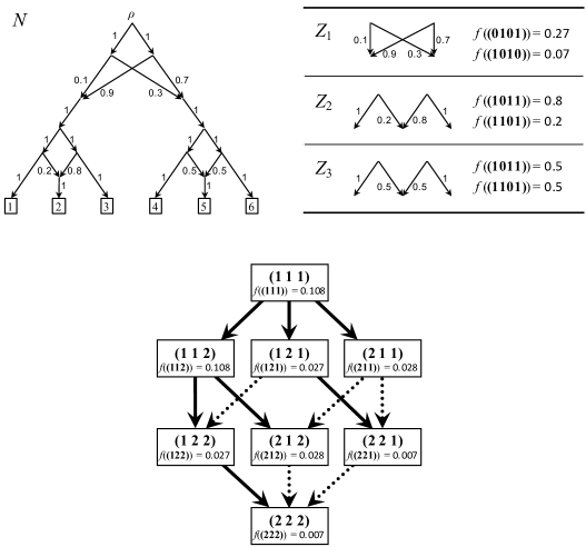
Figure 1. An illustration of Lemma 5.3. The top left is a tree-based phylogenetic $X$-network $N$ whose arcs are associated with probability. The top right shows the maximal zig-zag trails $Z_{i}$ in $N$ with $|\Omega_{i}|\geq 2$ and the likelihood of each element of $(\Omega_{i},\leq^{*})$ ($i=1,2,3$). On the bottom is the spanning tree $\Gamma$ (shown in bold) of the Hasse diagram of $(\Omega,\leq)$.

In what follows, for any $\Omega^{\prime}\subseteq\Omega$, we write $\it least(\Omega^{\prime})$ to mean the least element of $(\Omega^{\prime},\leq^{*})$. For any $\tau\in\Omega$, let ${\it Child}(\tau):=\{\tau^{\prime}\in V(\Gamma)\mid(\tau,\tau^{\prime})\in A(\Gamma)\}$ and $\it child^{*}(\tau):=least(Child(\tau))$. Also, for any $\tau^{\prime}\in\Omega\setminus\{\tau^{(1)}\}$, let $\it sibling^{*}(\tau^{\prime}):=least(\{\tau\in Child(parent(\tau^{\prime}))\mid\tau^{\prime}\leq^{*}\tau\land\tau\neq\tau^{\prime}\})$, where ${\it parent}(\tau^{\prime})$ represents a unique element $\tau\in V(\Gamma)$ with $(\tau,\tau^{\prime})\in A(\Gamma)$. We note that both $\it child^{*}(\tau^{\prime})=\emptyset$ and $\it sibling^{*}(\tau^{\prime})=\emptyset$ are possible to occur.

Lemma 5.4.

Let $\Gamma$ be the graph as in Lemma 5.3 and let $Q_{j}$ be a subset of $V(\Gamma)$ that is recursively defined by

$$Q_{j}:=\begin{cases}(Q_{j-1}\setminus\{\tau^{(j-1)}\})\cup\{\it child^{*}(\tau^{(j-1)}),\it sibling^{*}(\tau^{(j-1)})\}&j\in[2,k]\\ \{\tau^{(1)}\}&j=1.\end{cases}$$ (1)

Then, for each $j\in[1,k]$, we have $\tau^{(j)}\in Q_{j}$ and $\tau^{(\ell)}\not\in Q_{j}$ for all $\ell<j$.

Proof.

Let $P_{1}=Q_{1}$ and $P_{j}=\{\it least(Child(\tau)\setminus I_{j-1})\mid\tau\in I_{j-1}\}$ for $j\in[2,k]$. We will show that $P_{j}=Q_{j}$ holds for any $j\in[1,k]$, which completes the proof, since $\tau^{(j)}\in P_{j}$ and $\tau^{(\ell)}\not\in P_{j}$ for all $\ell<j$.

For $j\in[2,k]$, we have

$$P_{j} =\{\it least(Child(\tau)\setminus I_{j-1})\mid\tau\in I_{i-2}\}\cup\{\it least(Child(\tau^{(j-1)})\setminus I_{j-1})\}$$

$$=\{\it least(Child(\tau)\setminus I_{j-1})\mid\tau\in I_{j-2}\}\cup\{\it child^{*}(\tau^{(j-1)})\},$$

where we assume that $I_{0}=\emptyset$. Note that $I_{j-2}$ contains $p:={\it parent(\tau^{(j-1)})}$. This implies

$$P_{j} =\{\it least(Child(\tau)\setminus I_{j-1})\mid\tau\in I_{j-2}\setminus\{p\}\}\cup\{\it child^{*}(\tau^{(j-1)}),least(Child(p)\setminus I_{j-1})\}$$

$$=\{\it least(Child(\tau)\setminus I_{j-1})\mid\tau\in I_{j-2}\setminus\{p\}\}\cup\{\it child^{*}(\tau^{(j-1)}),sibling^{*}(\tau^{(j-1)})\}.$$

For any $\tau\in I_{j-2}\setminus\{p\}$, we have $\it least(Child(\tau)\setminus I_{j-1})=\it least(Child(\tau)\setminus I_{j-2})$ because $\tau^{(j-1)}\not\in\it Child(\tau)$ holds. We thus obtain

$$P_{j} =(\{\it least(Child(\tau)\setminus I_{j-2})\mid\tau\in I_{j-2}\}\setminus\{\it least(Child(p)\setminus I_{j-2})\})\cup\{\it child^{*}(\tau^{(j-1)}),\it sibling^{*}(\tau^{(j-1)})\}$$

$$=(P_{j-1}\setminus\{\tau^{(j-1)}\})\cup\{\it child^{*}(\tau^{(j-1)}),\it sibling^{*}(\tau^{(j-1)})\}.$$

From Equation (1) and $P_{1}=Q_{1}$, the desired conclusion follows. ∎

We are in a position to give an algorithm for Problem 4.1. As illustrated in Table 1, the algorithm starts by setting $j:=1$ and $Q_{1}:=\{\tau^{(1)}\}$ and then returns $\tau^{(j)}={\it least}(Q_{j})$ for each $j\in[1,k]$, where $Q_{j}$ is iteratively updated using Equation (1).

Table 1. Application of the proposed algorithm to the input $N$ in Figure 1 ($k=8$).

	$j=1$	$j=2$	$j=3$	$j=4$	$j=5$	$j=6$	$j=7$	$j=8$
$Q_{j}$	$\{(1\;1\;1)\}$	$\{(1\;1\;2)\}$	$\{(2\;1\;1),(2\;1\;2)\}$	$\{(1\;2\;1),(2\;1\;2)\}$	$\{(1\;2\;1),(1\;2\;2)\}$	$\{(1\;2\;2),(2\;2\;1)\}$	$\{(2\;2\;1),(2\;2\;2)\}$	$\{(2\;2\;2)\}$
$\tau^{(j)}$	$(1\;1\;1)$	$(1\;1\;2)$	$(2\;1\;1)$	$(2\;1\;2)$	$(1\;2\;1)$	$(1\;2\;2)$	$(2\;2\;1)$	$(2\;2\;2)$
$\it child^{*}(\tau^{(j)})$	$(1\;1\;2)$	$(2\;1\;2)$	$\emptyset$	$\emptyset$	$(2\;2\;1)$	$(2\;2\;2)$	$\emptyset$
$\it sibling^{*}(\tau^{(j)})$	$\emptyset$	$(2\;1\;1)$	$(1\;2\;1)$	$(1\;2\;2)$	$\emptyset$	$\emptyset$	$\emptyset$

In order to analyse the running time of the above algorithm, let us review some basics of a priority queue, which is a data structure for maintaining objects that are prioritised by their associated values. In its most basic form, a priority queue supports the operations called Insert and Delete-min, where the former refers to adding a new object, and the latter to detecting and deleting the one with the highest-priority [2]. Implemented with a binary heap, each of these operations can be performed in $O(\log n)$ time, where $n$ denotes the number of the elements in the priority queue [2].

Theorem 5.5.

The top-$k$ support tree ranking problem (Problem 4.1) can be solved with linear delay, and hence in $O(k|A(N)|)$ time.

Proof.

As Equation (1) implies that $|Q_{j+1}-Q_{j}|\leq 1$ holds for any $j\in[1,k-1]$, $|Q_{j}|\leq k$ holds for any $j\in[1,k]$. Then, if we keep the elements of each $Q_{j}$ in a priority queue, $O(\log k)$ time suffices to return $\tau^{(j)}$ and to delete $\tau^{(j)}$ from $Q_{j}$. Also, once $\it child^{*}(\tau^{(j)})$ and $\it sibling^{*}(\tau^{(j)})$ have been obtained, inserting the two elements requires $O(\log k)$ time. We note that $O(\log k)\leq O(|A(N)|)$ follows from $k\leq 2^{|A(N)|}$. By Proposition 5.1, for each $j\in[1,k-1]$, one can compute $\{\it child^{*}(\tau^{(j)}),\it sibling^{*}(\tau^{(j)})\}$ in $\sum_{i=1}^{d}{O(|A(Z_{i})|)}$ time, which equals $O(|A(N)|)$ time as $\{Z_{1},\dots,Z_{d}\}$ is a decomposition of $N$. Hence, our algorithm can return $\tau^{(1)},\dots,\tau^{(k)}$ one after the other in such a way that the delay between two consecutive outputs is $O(|A(N)|)$ time. This completes the proof. ∎

Finally, we make two remarks. First, $\Omega(k|A(N)|)$ time is required to output $k$ distinct support trees of $N$ as each support tree has size $\Omega(|A(N)|)$. Therefore, the running time of our algorithm (as well as that of the enumeration algorithm in [8]) is $\Theta(k|A(N)|)$, which guarantees the optimality of those algorithms. Second, as commonly in the literature (e.g., [10]), it would be natural to wonder about the time complexity of an analogue of Problem 4.1 that only asks for outputting a sequence of the differences between $\tau^{(j-1)}$ and $\tau^{(j)}$; however, we note that this problem still requires $\Omega(k|A(N)|)$ time because the size of each difference is $\Omega(|A(N)|)$. To illustrate this, consider a tree-based phylogenetic $X$-network $N$ that is decomposed into maximal fences, each of which has only one admissible arc-set, and $c$ crowns, each of which has size $\Omega(|A(N)|/c)$. The difference between any two support trees has size $\Omega(|A(N)|/c)$, which equals $\Omega(|A(N)|)$ if $c$ is a constant.

References

- [1] M. Anaya, O. Anipchenko-Ulaj, A. Ashfaq, J. Chiu, M. Kaiser, M. S. Ohsawa, M. Owen, E. Pavlechko, K. St. John, S. Suleria, K. Thompson, and C. Yap, On determining if tree-based networks contain fixed trees, Bulletin of Mathematical Biology 78 (2016), no. 5, 961–969.
- [2] T. H. Cormen, C. E. Leiserson, R. L. Rivest, and C. Stein, Introduction to algorithms, MIT press, 2009.
- [3] M. Fischer, M. Galla, L. Herbst, Y. Long, and K. Wicke, Non-binary treebased unrooted phylogenetic networks and their relations to binary and rooted ones, arXiv:1810.06853 [q-bio.PE] (2018).
- [4] A. Francis, K. T. Huber, and V. Moulton, Tree-based unrooted phylogenetic networks, Bulletin of mathematical biology 80 (2018), no. 2, 404–416.
- [5] A. Francis, C. Semple, and M. Steel, New characterisations of tree-based networks and proximity measures, Advances in Applied Mathematics 93 (2018), 93–107.
- [6] A. R. Francis and M. Steel, Which phylogenetic networks are merely trees with additional arcs?, Systematic Biology 64 (2015), no. 5, 768–777.
- [7] M. Hayamizu, On the existence of infinitely many universal tree-based networks, Journal of Theoretical Biology 396 (2016), 204–206.
- [8] by same author, A structure theorem for tree-based phylogenetic networks, arXiv:1811.05849 [math.CO] (2018).
- [9] D. H. Huson, R. Rupp, and C. Scornavacca, Phylogenetic networks: concepts, algorithms and applications, Cambridge University Press, 2010.
- [10] S. Kapoor and H. Ramesh, Algorithms for enumerating all spanning trees of undirected and weighted graphs, SIAM Journal on Computing 24 (1995), no. 2, 247–265.
- [11] J. C. Pons, C. Semple, and M. Steel, Tree-based networks: characterisations, metrics, and support trees, Journal of Mathematical Biology 78 (2019), no. 4, 899–918.
- [12] L. van Iersel, Different topological restrictions of rooted phylogenetic networks. Which make biological sense?, http://phylonetworks.blogspot.nl/2013/03/different-topological-restrictions-of.html, 2013, Accessed: 2019-03-16.
- [13] L. Zhang, On tree-based phylogenetic networks, Journal of Computational Biology 23 (2016), no. 7, 553–565.
Acknowledgement
The first author acknowledges support from JST PRESTO Grant Number JPMJPR16EB.